A Gibbs Sampler for Multivariate Linear Regression

Abstract

Kelly (2007, hereafter K07) described an efficient algorithm, using Gibbs sampling, for performing linear regression in the fairly general case where non-zero measurement errors exist for both the covariates and response variables, where these measurements may be correlated (for the same data point), where the response variable is affected by intrinsic scatter in addition to measurement error, and where the prior distribution of covariates is modeled by a flexible mixture of Gaussians rather than assumed to be uniform. Here I extend the K07 algorithm in two ways. First, the procedure is generalized to the case of multiple response variables. Second, I describe how to model the prior distribution of covariates using a Dirichlet process, which can be thought of as a Gaussian mixture where the number of mixture components is learned from the data. I present an example of multivariate regression using the extended algorithm, namely fitting scaling relations of the gas mass, temperature, and luminosity of dynamically relaxed galaxy clusters as a function of their mass and redshift. An implementation of the Gibbs sampler in the r language, called lrgs, is provided.

1 Introduction

Linear regression is perhaps the most widely used example of parameter fitting throughout the sciences. Yet, the traditional ordinary least-squares (or weighted least-squares) approach to regression neglects some features that are practically ubiquitous in astrophysical data, namely the existence of measurement errors, often correlated with one another, on all quantities of interest, and the presence of residual, intrinsic scatter (i.e. physical scatter, not the result of measurement errors) about the best fit. K07 takes on this problem (see that work for a more extensive overview of the prior literature) by devising an efficient algorithm for simultaneously constraining the parameters of a linear model and the intrinsic scatter in the presence of such heteroscedastic and correlated measurement errors. In addition, the K07 approach corrects a bias that exists when the underlying distribution of covariates in a regression is assumed to be uniform, by modeling this distribution as a flexible mixture of Gaussian (normal) distributions and marginalizing over it.

The K07 model is considerably more complex, in terms of the number of free parameters, than traditional regression. Nevertheless, it can be efficiently constrained using a fully conjugate Gibbs sampler, as described in that work. Briefly, the approach takes advantage of the fact that, for a suitable model, the fully conditional posterior of certain parameters (or blocks of parameters) may be expressible as a known distribution which can be sampled from directly using standard numerical techniques. If all model parameters can be sampled this way, then a Gibbs sampler, which simply cycles through the list of parameters, updating or block-updating them in turn, can move efficiently through the parameter space. By repeatedly Gibbs sampling, a Markov chain that converges to the joint posterior distribution of all model parameters is generated (see, e.g., Gelman et al. 2004 for theoretical background). The individual pieces (e.g., the model distributions of measurement error, intrinsic scatter, and the covariate prior distribution) of the K07 model are conjugate, making it suitable for this type of efficient Gibbs sampling. This is a key advantage in terms of making the resulting algorithm widely accessible to the community, since conjugate Gibbs samplers, unlike more general and powerful Markov Chain Monte Carlo samplers, require no a priori tuning by the user.

While K07 argue against the assumption of a uniform prior for covariates, it should be noted that the alternative of a Gaussian mixture model (or the Dirichlet process generalization introduced below) is not necessarily applicable in every situation either. When a well motivated physical model of the distribution of covariates exists, it may well be preferable to use it, even at the expense of computational efficiency. In the general case, we can hope that a flexible parametrization like the Gaussian mixture is adequate, although it is always worth checking a posteriori that the model distribution of covariates provides a good description of the data. K07 and Sereno & Ettori (2015) discuss real applications in which a Gaussian distribution of covariates turns out to be adequate, despite the underlying physics being non-Gaussian.

This work describes two useful generalizations to the K07 algorithm. First, the number of response variables is allowed to be greater than one. Second, the prior distribution of covariates may be modeled using a Dirichlet process rather than as a mixture of Gaussians with a fixed number of components. A Dirichlet process describes a probability distribution over the space of probability distributions, and (in contrast to the many parameters required to specify a large mixing model) is described only by a concentration parameter and a base distribution. For the choice of a Gaussian base distribution, used here, the Dirichlet process can be thought of as a Gaussian mixture in which the number of mixture components is learned from the data and marginalized over as the fit progresses (see more discussion, in a different astrophysical context, by Schneider et al. 2015). This makes it a very general and powerful alternative to the standard fixed-size Gaussian mixture, as well as one that requires even less tuning by the user, since the number of mixture components need not be specified. Crucially, both of these generalizations preserve the conjugacy of the model, so that posterior samples can still be easily obtained by Gibbs sampling.

Of course, K07 (or this paper) does not provide the only implementation of conjugate Gibbs sampling, nor is that approach the only one possible for linear regression in the Bayesian context. Indeed, there exist more general statistical packages capable of identifying conjugate sampling strategies (where possible) based on an abstract model definition (e.g., bugs, jags, and stan). The use of more general Markov chain sampling techniques naturally allow for more general (non-conjugate) models and/or parametrizations (e.g., Maughan 2014; Robotham & Obreschkow 2015). Nevertheless, there is something appealing in the relative simplicity of implementation and use of the conjugate Gibbs approach, particularly as it applies so readily to the commonly used linear model with Gaussian scatter.

Section 2 describes the model employed in this work in more detail, and introduces notation. Section 3 outlines the changes to the K07 sampling algorithm needed to accomodate the generalizations above. Since this work is intended to extend that of K07, I confine this discussion only to steps which differ from the that algorithm, and do not review the Gibbs sampling procedure in its entirety. However, the level of detail is intentionally high; between this document and K07, it should be straightforward for the interested reader to create his or her own implementation of the entire algorithm. Section 4 provides some example analyses, including one with real astrophysical data, and discusses some practical aspects of the approach.

The complete algorithm described here (with both Gaussian mixture and Dirichlet process models) has been implemented in the r language. The package is named Linear Regression by Gibbs Sampling (lrgs), the better to sow confusion among extragalactic astronomers. The code can be obtained from GitHub or the Comprehensive R Archive Network.

2 Model and Notation

Here I review the model described by K07, introducing the generalization to multiple response variables (Section 2.1) and the use of the Dirichlet process to describe the prior distribution of the covariates (Section 2.2). The notation used here is summarized in Table 1; it differs slightly from that of K07, as noted. In this document, $A\sim B$ denotes a stochastic relationship in which a random variable $A$ is drawn from the probability distribution $B$, and boldface distinguishes vector- or matrix-valued variables.

Table 1: Summary of notation used in this work. Where this departs from the notation used by K07, the K07 equivalent is noted in the last column.

	Symbol	Meaning	K07
General	$\mathcal{N}_{\nu}({\mathchoice{\hbox{$\displaystyle\mu$}}{\hbox{$\textstyle\mu$}}{\hbox{$\scriptstyle\mu$}}{\hbox{$\scriptscriptstyle\mu$}}},{\mathchoice{\hbox{$\displaystyle\Sigma$}}{\hbox{$\textstyle\Sigma$}}{\hbox{$\scriptstyle\Sigma$}}{\hbox{$\scriptscriptstyle\Sigma$}}})$	$\nu$-dimensional normal distribution (mean $\textstyle\mu$, covariance $\textstyle\Sigma$)
notation	$\mathcal{W}({\mathchoice{\hbox{$\displaystyle V$}}{\hbox{$\textstyle V$}}{\hbox{$\scriptstyle V$}}{\hbox{$\scriptscriptstyle V$}}},\nu)$	Wishart distribution (scale matrix $\textstyle V$, $\nu$ degrees of freedom)
	$A_{ij}$	single element of matrix $\textstyle A$
	${\mathchoice{\hbox{$\displaystyle A_{j\cdot}$}}{\hbox{$\textstyle A_{j\cdot}$}}{\hbox{$\scriptstyle A_{j\cdot}$}}{\hbox{$\scriptscriptstyle A_{j\cdot}$}}},{\mathchoice{\hbox{$\displaystyle A_{\cdot j}$}}{\hbox{$\textstyle A_{\cdot j}$}}{\hbox{$\scriptstyle A_{\cdot j}$}}{\hbox{$\scriptscriptstyle A_{\cdot j}$}}}$	$j$th row or column of $\textstyle A$
	${\mathchoice{\hbox{$\displaystyle A_{\bar{j}\cdot}$}}{\hbox{$\textstyle A_{\bar{j}\cdot}$}}{\hbox{$\scriptstyle A_{\bar{j}\cdot}$}}{\hbox{$\scriptscriptstyle A_{\bar{j}\cdot}$}}},{\mathchoice{\hbox{$\displaystyle A_{\cdot\bar{j}}$}}{\hbox{$\textstyle A_{\cdot\bar{j}}$}}{\hbox{$\scriptstyle A_{\cdot\bar{j}}$}}{\hbox{$\scriptscriptstyle A_{\cdot\bar{j}}$}}}$	$\textstyle A$ with the $j$th row or column removed	${\mathchoice{\hbox{$\displaystyle A_{-j\cdot}$}}{\hbox{$\textstyle A_{-j\cdot}$}}{\hbox{$\scriptstyle A_{-j\cdot}$}}{\hbox{$\scriptscriptstyle A_{-j\cdot}$}}},{\mathchoice{\hbox{$\displaystyle A_{\cdot-j}$}}{\hbox{$\textstyle A_{\cdot-j}$}}{\hbox{$\scriptstyle A_{\cdot-j}$}}{\hbox{$\scriptscriptstyle A_{\cdot-j}$}}}$
	$\mathbf{1}_{n}$	$n\times n$ identity matrix
Common	$n$	number of data points
parameters	$p$	number of covariates
	$m$	number of responses	1
	$K$	number of Gaussian mixture components or clusters
	${\mathchoice{\hbox{$\displaystyle x_{i}$}}{\hbox{$\textstyle x_{i}$}}{\hbox{$\scriptstyle x_{i}$}}{\hbox{$\scriptscriptstyle x_{i}$}}},{\mathchoice{\hbox{$\displaystyle y_{i}$}}{\hbox{$\textstyle y_{i}$}}{\hbox{$\scriptstyle y_{i}$}}{\hbox{$\scriptscriptstyle y_{i}$}}}$	measured covariates and responses for data point $i$
	$\textstyle M_{i}$	measurement covariance matrix for data point $i$	$\textstyle\Sigma_{i}$
	${\mathchoice{\hbox{$\displaystyle\xi_{i}$}}{\hbox{$\textstyle\xi_{i}$}}{\hbox{$\scriptstyle\xi_{i}$}}{\hbox{$\scriptscriptstyle\xi_{i}$}}},{\mathchoice{\hbox{$\displaystyle\eta_{i}$}}{\hbox{$\textstyle\eta_{i}$}}{\hbox{$\scriptstyle\eta_{i}$}}{\hbox{$\scriptscriptstyle\eta_{i}$}}}$	true covariates and responses for data point $i$
	$\textstyle\alpha$	intercepts of the linear model
	$\textstyle\beta$	slopes of the linear model
	$\textstyle\Sigma$	intrinsic covariance about the linear model	$\sigma^{2}$
	$\textstyle G$	mixture component/cluster identification for each data point
Gaussian	$\textstyle\pi$	weight of the each mixture component
mixture	$\textstyle\mu_{k}$	mean of the $k$th component
	$\textstyle T_{k}$	covariance of the $k$th component
	$\textstyle\mu_{0}$	mean of the prior distribution of each $\textstyle\mu_{k}$
	$\textstyle U$	covariance of the prior distribution of each $\textstyle\mu_{k}$
	$\textstyle W$	scale matrix of the prior distribution of each $\textstyle T_{k}$
Dirichlet	$\textstyle\mu$	mean of the normal base distribution
process	$\textstyle T$	covariance of the normal base distribution
	$\kappa$	concentration parameter of the process
	$a$	shape parameter of the prior of $\kappa$
	$b$	rate parameter of the prior of $\kappa$

2.1 Gaussian mixture model

We are interested in $p+m$ properties of some class of object, where $p$ of these (covariates) are supposed to be physically responsible for determining the other $m$ (response variables). Measurements of these $p+m$ quantities have been gathered for $n$ objects. The true values of the covariates for the $i$th data point are denoted $\textstyle\xi_{i}$, and the corresponding true responses are denoted $\textstyle\eta_{i}$; these are nuisance parameters that will be marginalized over. The measured values of the corresponding quantities are denoted $\textstyle x_{i}$ and $\textstyle y_{i}$, and are assumed to be related to the true values by a $(p+m)$-dimensional normal measurement error distribution, which may be different for each data point. Writing the $\nu$-dimensional normal distribution with mean $\textstyle\mu$ and covariance $\textstyle V$ as $\mathcal{N}_{\nu}({\mathchoice{\hbox{$\displaystyle\mu$}}{\hbox{$\textstyle\mu$}}{\hbox{$\scriptstyle\mu$}}{\hbox{$\scriptscriptstyle\mu$}}},{\mathchoice{\hbox{$\displaystyle V$}}{\hbox{$\textstyle V$}}{\hbox{$\scriptstyle V$}}{\hbox{$\scriptscriptstyle V$}}})$, this is (for the $i$th data point)

$$\left(\begin{array}[]{c}{\mathchoice{\hbox{$\displaystyle x_{i}$}}{\hbox{$\textstyle x_{i}$}}{\hbox{$\scriptstyle x_{i}$}}{\hbox{$\scriptscriptstyle x_{i}$}}}\\ {\mathchoice{\hbox{$\displaystyle y_{i}$}}{\hbox{$\textstyle y_{i}$}}{\hbox{$\scriptstyle y_{i}$}}{\hbox{$\scriptscriptstyle y_{i}$}}}\end{array}\right)\sim\mathcal{N}_{p+m}\left[\left(\begin{array}[]{c}{\mathchoice{\hbox{$\displaystyle\xi_{i}$}}{\hbox{$\textstyle\xi_{i}$}}{\hbox{$\scriptstyle\xi_{i}$}}{\hbox{$\scriptscriptstyle\xi_{i}$}}}\\ {\mathchoice{\hbox{$\displaystyle\eta_{i}$}}{\hbox{$\textstyle\eta_{i}$}}{\hbox{$\scriptstyle\eta_{i}$}}{\hbox{$\scriptscriptstyle\eta_{i}$}}}\end{array}\right),\,{\mathchoice{\hbox{$\displaystyle M_{i}$}}{\hbox{$\textstyle M_{i}$}}{\hbox{$\scriptstyle M_{i}$}}{\hbox{$\scriptscriptstyle M_{i}$}}}\right].$$ (1)

The $p$-dimensional distribution of covariates that these objects originally come from is not necessarily uniform. It is therefore modeled in a flexible way, as a mixture of $K$ $p$-dimensional normal distributions,

$${\mathchoice{\hbox{$\displaystyle\xi_{i}$}}{\hbox{$\textstyle\xi_{i}$}}{\hbox{$\scriptstyle\xi_{i}$}}{\hbox{$\scriptscriptstyle\xi_{i}$}}}\sim\sum_{k=1}^{K}\pi_{k}\,\mathcal{N}_{p}\left({\mathchoice{\hbox{$\displaystyle\mu_{k}$}}{\hbox{$\textstyle\mu_{k}$}}{\hbox{$\scriptstyle\mu_{k}$}}{\hbox{$\scriptscriptstyle\mu_{k}$}}},\,{\mathchoice{\hbox{$\displaystyle T_{k}$}}{\hbox{$\textstyle T_{k}$}}{\hbox{$\scriptstyle T_{k}$}}{\hbox{$\scriptscriptstyle T_{k}$}}}\right),$$ (2)

with $\sum_{k}\pi_{k}=1$. The summation notation in Equation 2 is meant to convey that $\textstyle\xi_{i}$ is drawn from the $k$th normal distribution (which has mean $\textstyle\mu_{k}$ and covariance $\textstyle T_{k}$) with probability $\pi_{k}$. As in K07, this is implemented by means of a set of latent indicator variables, $\textstyle G$, with $G_{i}$ indicating which of the $K$ mixture components $\textstyle\xi_{i}$ is drawn from. Formally, each $\textstyle G$ follows the multinomial distribution defined by the proportions $\textstyle\pi$.

The parameters $\textstyle G$, $\textstyle\pi$, $\{{\mathchoice{\hbox{$\displaystyle\mu_{k}$}}{\hbox{$\textstyle\mu_{k}$}}{\hbox{$\scriptstyle\mu_{k}$}}{\hbox{$\scriptscriptstyle\mu_{k}$}}}\}$ and $\{{\mathchoice{\hbox{$\displaystyle T_{k}$}}{\hbox{$\textstyle T_{k}$}}{\hbox{$\scriptstyle T_{k}$}}{\hbox{$\scriptscriptstyle T_{k}$}}}\}$ can be learned from the data, but it is helpful to impose some structure on them. Therefore, we adopt a hierarchical model whereby the vectors $\{{\mathchoice{\hbox{$\displaystyle\mu_{k}$}}{\hbox{$\textstyle\mu_{k}$}}{\hbox{$\scriptstyle\mu_{k}$}}{\hbox{$\scriptscriptstyle\mu_{k}$}}}\}$ themselves follow a normal distribution,

$${\mathchoice{\hbox{$\displaystyle\mu_{k}$}}{\hbox{$\textstyle\mu_{k}$}}{\hbox{$\scriptstyle\mu_{k}$}}{\hbox{$\scriptscriptstyle\mu_{k}$}}}\sim\mathcal{N}_{p}\left({\mathchoice{\hbox{$\displaystyle\mu_{0}$}}{\hbox{$\textstyle\mu_{0}$}}{\hbox{$\scriptstyle\mu_{0}$}}{\hbox{$\scriptscriptstyle\mu_{0}$}}},\,{\mathchoice{\hbox{$\displaystyle U$}}{\hbox{$\textstyle U$}}{\hbox{$\scriptstyle U$}}{\hbox{$\scriptscriptstyle U$}}}\right),$$ (3)

and both $\textstyle U$ and the covariances $\{{\mathchoice{\hbox{$\displaystyle T_{k}$}}{\hbox{$\textstyle T_{k}$}}{\hbox{$\scriptstyle T_{k}$}}{\hbox{$\scriptscriptstyle T_{k}$}}}\}$ follow inverse-Wishart distributions,

$$U \sim \mathcal{W}^{-1}\left({\mathchoice{\hbox{$\displaystyle W$}}{\hbox{$\textstyle W$}}{\hbox{$\scriptstyle W$}}{\hbox{$\scriptscriptstyle W$}}},K+p\right),$$ (4)

$$T_{k} \sim \mathcal{W}^{-1}\left({\mathchoice{\hbox{$\displaystyle W$}}{\hbox{$\textstyle W$}}{\hbox{$\scriptstyle W$}}{\hbox{$\scriptscriptstyle W$}}},\,K+p\right).$$

Here $\mathcal{W}^{-1}({\mathchoice{\hbox{$\displaystyle V$}}{\hbox{$\textstyle V$}}{\hbox{$\scriptstyle V$}}{\hbox{$\scriptscriptstyle V$}}},\nu)$ denotes the inverse-Wishart distribution with scale matrix $\textstyle V$ and $\nu$ degrees of freedom. I follow K07 in taking uniform priors on the hyperparameters $\textstyle\mu_{0}$ and $\textstyle W$. Note that this hierarchical model, and the Gaussian mixture itself, is fairly flexible but not fully general. While these are typically reasonable assumptions when we have little prior information about the distribution of covariates, they may not be appropriate for all situations. The particular structure in Equations 3–4 tends to promote compactness in the covariate distribution; that is, if multiple, well separated clusters of covariates exist, the onus is on the data to show that they are required.

The relationship by which the $p$ covariates determine the $m$ responses is assumed to be linear, with a normal intrinsic scatter,

$${\mathchoice{\hbox{$\displaystyle\eta_{i}$}}{\hbox{$\textstyle\eta_{i}$}}{\hbox{$\scriptstyle\eta_{i}$}}{\hbox{$\scriptscriptstyle\eta_{i}$}}}\sim\mathcal{N}_{m}\left({\mathchoice{\hbox{$\displaystyle\alpha$}}{\hbox{$\textstyle\alpha$}}{\hbox{$\scriptstyle\alpha$}}{\hbox{$\scriptscriptstyle\alpha$}}}+{\mathchoice{\hbox{$\displaystyle\beta$}}{\hbox{$\textstyle\beta$}}{\hbox{$\scriptstyle\beta$}}{\hbox{$\scriptscriptstyle\beta$}}}{\mathchoice{\hbox{$\displaystyle\xi_{i}$}}{\hbox{$\textstyle\xi_{i}$}}{\hbox{$\scriptstyle\xi_{i}$}}{\hbox{$\scriptscriptstyle\xi_{i}$}}},\,{\mathchoice{\hbox{$\displaystyle\Sigma$}}{\hbox{$\textstyle\Sigma$}}{\hbox{$\scriptstyle\Sigma$}}{\hbox{$\scriptscriptstyle\Sigma$}}}\right).$$ (5)

Note that the linearity of the mean is crucial to maintaining the conjugacy of the model. Here $\textstyle\alpha$ is the $m\times 1$ vector of intercepts, $\textstyle\beta$ is an $m\times p$ matrix of slopes linking each response variable with each of the covariates, and $\textstyle\Sigma$ is the $m\times m$ intrinsic covariance matrix (assumed to be constant with respect to $\textstyle\xi$). This can be written compactly for the entire data set in matrix form, with the definitions

$$X_{i\cdot} = (1,\,{\mathchoice{\hbox{$\displaystyle\xi_{i}$}}{\hbox{$\textstyle\xi_{i}$}}{\hbox{$\scriptstyle\xi_{i}$}}{\hbox{$\scriptscriptstyle\xi_{i}$}}}^{\mathrm{T}}),$$ (6)

$$Y_{i\cdot} = {\mathchoice{\hbox{$\displaystyle\eta_{i}$}}{\hbox{$\textstyle\eta_{i}$}}{\hbox{$\scriptstyle\eta_{i}$}}{\hbox{$\scriptscriptstyle\eta_{i}$}}}^{\mathrm{T}},$$

$$B = ({\mathchoice{\hbox{$\displaystyle\alpha$}}{\hbox{$\textstyle\alpha$}}{\hbox{$\scriptstyle\alpha$}}{\hbox{$\scriptscriptstyle\alpha$}}},\,{\mathchoice{\hbox{$\displaystyle\beta$}}{\hbox{$\textstyle\beta$}}{\hbox{$\scriptstyle\beta$}}{\hbox{$\scriptscriptstyle\beta$}}})^{\mathrm{T}}.$$

where $\textstyle Y$ is $n\times m$, $\textstyle X$ is $n\times(p+1)$, and $\textstyle B$ is $(p+1)\times m$. The notation $\textstyle A_{i\cdot}$ refers to the $i$th row of $A$; likewise $\textstyle A_{\cdot j}$ would refer to the $j$th column. The statement of the linear model then takes the familiar form

$$Y = {\mathchoice{\hbox{$\displaystyle XB$}}{\hbox{$\textstyle XB$}}{\hbox{$\scriptstyle XB$}}{\hbox{$\scriptscriptstyle XB$}}}+{\mathchoice{\hbox{$\displaystyle E$}}{\hbox{$\textstyle E$}}{\hbox{$\scriptstyle E$}}{\hbox{$\scriptscriptstyle E$}}},$$ (7)

$$E_{i\cdot} \sim \mathcal{N}_{m}\left({\mathchoice{\hbox{$\displaystyle 0$}}{\hbox{$\textstyle 0$}}{\hbox{$\scriptstyle 0$}}{\hbox{$\scriptscriptstyle 0$}}},\,{\mathchoice{\hbox{$\displaystyle\Sigma$}}{\hbox{$\textstyle\Sigma$}}{\hbox{$\scriptstyle\Sigma$}}{\hbox{$\scriptscriptstyle\Sigma$}}}\right).$$

As noted in Sections 3.1.3 and 3.1.4, the conjugate prior distributions for $\textstyle B$ and $\textstyle\Sigma$ are, respectively, normal and inverse-Wishart.

2.2 Dirichlet process model

The Gaussian mixture prior on the distribution of covariates is flexible, but requires us to either chose a number of mixture components outright or carefully check that the sensitivity of results to the number of components. Alternatively, we can constrain the distribution of covariates using a Dirichlet process, which describes a probability distribution over probability distributions. A Dirichlet process is defined by a concentration parameter, $\kappa$, and a base distribution, $P_{0}$. By choosing $P_{0}$ to be $p$-dimensional normal, the conjugacy relations that made the Gaussian mixture efficient to Gibbs sample will also hold for the Dirichlet process. Used in this way, the Dirichlet process can be thought of as a Gaussian mixture in which the number of components is marginalized over (Neal 2000 and references therein). The analog of Equation 2 is generally written

$$\xi_{i} \sim P,$$ (8)

$$P \sim \mathrm{DP}(P_{0},\kappa),$$

$$P_{0} = \mathcal{N}_{p}({\mathchoice{\hbox{$\displaystyle\mu$}}{\hbox{$\textstyle\mu$}}{\hbox{$\scriptstyle\mu$}}{\hbox{$\scriptscriptstyle\mu$}}},{\mathchoice{\hbox{$\displaystyle T$}}{\hbox{$\textstyle T$}}{\hbox{$\scriptstyle T$}}{\hbox{$\scriptscriptstyle T$}}}).$$

Here $\textstyle\mu$ and $\textstyle T$ are the hyperparameters of the base distribution, for which I assume uniform priors. Note that there is only one $\textstyle\mu$ and one $\textstyle T$, unlike in the Gaussian mixture model, and there is no analog of $\textstyle\mu_{0}$, $\textstyle U$ or $\textstyle W$. The remainder of the model, namely Equations 1 and 5–7, is the same as above.

In practice, for a given realization of the model parameters, the algorithm for realizing the Dirichlet process divides the data set into a finite number of clusters, with points in each cluster having identical values of $\textstyle\xi$. The vector of labels $\textstyle G$ will identify which cluster each data point belongs to, similarly to its use in Section 2.1. A vector of cluster proportions, $\textstyle\pi$, could also be defined analogously. However, in practice, the procedure for Gibbs sampling the Dirichlet process model implicitly marginalizes over it, and so $\textstyle\pi$ never explicitly appears in the calculations (Section 3.2).

The concentration parameter of the Dirichlet process is related to the number of clusters in the data set, and can also be marginalized over. The conjugate prior for $\kappa$ is the Gamma distribution,

$$\kappa\sim\mathrm{Gamma}(a,b),$$ (9)

where $a$ and $b$ are respectively the shape and rate parameters of the prior. If the approximate number of clusters in the data set is known, these parameters can be chosen accordingly; otherwise, they can be chosen to be minimally informative (see discussion by Dorazio 2009 and Murugiah & Sweeting 2012, and Section 4.1).

3 The Gibbs Sampler

Both of the models described above can be efficiently Gibbs sampled because they are fully conjugate. Recall that, in this situation, the sampling algorithm can be entirely specified as the set of conditional distributions used to sequentially update each parameter or block of parameters. Section 3.1 summarizes the changes to the K07 procedure needed to sample the Gaussian mixture model when there are multiple response variables, and Section 3.2 describes the procedure for sampling the Dirichlet process model.

In either case, an initial guess is needed for most of the free parameters, but this need not be very sophisticated. For example, it is generally acceptable to begin with the values of $\{{\mathchoice{\hbox{$\displaystyle\xi_{i}$}}{\hbox{$\textstyle\xi_{i}$}}{\hbox{$\scriptstyle\xi_{i}$}}{\hbox{$\scriptscriptstyle\xi_{i}$}}}\}$ and $\{{\mathchoice{\hbox{$\displaystyle\eta_{i}$}}{\hbox{$\textstyle\eta_{i}$}}{\hbox{$\scriptstyle\eta_{i}$}}{\hbox{$\scriptscriptstyle\eta_{i}$}}}\}$ respectively initialized to the measured values $\{{\mathchoice{\hbox{$\displaystyle x_{i}$}}{\hbox{$\textstyle x_{i}$}}{\hbox{$\scriptstyle x_{i}$}}{\hbox{$\scriptscriptstyle x_{i}$}}}\}$ and $\{{\mathchoice{\hbox{$\displaystyle y_{i}$}}{\hbox{$\textstyle y_{i}$}}{\hbox{$\scriptstyle y_{i}$}}{\hbox{$\scriptscriptstyle y_{i}$}}}\}$, the intercepts $\textstyle\alpha$ set to the average value of each column of $\textstyle Y$, and the slopes $\textstyle\beta$ set to zero. Of course, more intelligent guesses will decrease the “burn-in” time of the resulting Markov chain, but generally this is relatively short.

3.1 Sampling the Gaussian mixture model

The procedure for updating the parameters governing the distribution of covariates ($\textstyle G$, $\textstyle\pi$, $\{{\mathchoice{\hbox{$\displaystyle\mu_{k}$}}{\hbox{$\textstyle\mu_{k}$}}{\hbox{$\scriptstyle\mu_{k}$}}{\hbox{$\scriptscriptstyle\mu_{k}$}}}\}$, $\{{\mathchoice{\hbox{$\displaystyle T_{k}$}}{\hbox{$\textstyle T_{k}$}}{\hbox{$\scriptstyle T_{k}$}}{\hbox{$\scriptscriptstyle T_{k}$}}}\}$, $\textstyle\mu_{0}$, $\textstyle U$ and $\textstyle W$, for which I adopt the same priors as K07) is not affected by the generalization to multiple responses, and the reader is referred to K07 for the details of those updates. Here, I review the procedure for Gibbs sampling the true values of the covariates and responses for each data point, $\{{\mathchoice{\hbox{$\displaystyle\xi_{i}$}}{\hbox{$\textstyle\xi_{i}$}}{\hbox{$\scriptstyle\xi_{i}$}}{\hbox{$\scriptscriptstyle\xi_{i}$}}}\}$ and $\{{\mathchoice{\hbox{$\displaystyle\eta_{i}$}}{\hbox{$\textstyle\eta_{i}$}}{\hbox{$\scriptstyle\eta_{i}$}}{\hbox{$\scriptscriptstyle\eta_{i}$}}}\}$, the regression coefficients, $\textstyle\alpha$ and $\textstyle\beta$, and the intrinsic covariance matrix, $\textstyle\Sigma$.

3.1.1 Updating the covariates

See Equations 59–65 of K07 for the corresponding discussion in that work. The fully conditional posterior of the $j$th covariate ($j=1,2,\ldots,p$) for data point $i$ is

$$({\mathchoice{\hbox{$\displaystyle\xi_{i}$}}{\hbox{$\textstyle\xi_{i}$}}{\hbox{$\scriptstyle\xi_{i}$}}{\hbox{$\scriptscriptstyle\xi_{i}$}}})_{j}|\ldots\sim\mathcal{N}_{1}\left(\hat{\xi}_{(ij)},\sigma_{(ij)}^{2}\right),$$ (10)

where

$$\sigma_{(ij)}^{2} = \left[({\mathchoice{\hbox{$\displaystyle M_{i}$}}{\hbox{$\textstyle M_{i}$}}{\hbox{$\scriptstyle M_{i}$}}{\hbox{$\scriptscriptstyle M_{i}$}}}^{-1})_{jj}+({\mathchoice{\hbox{$\displaystyle T_{G_{i}}$}}{\hbox{$\textstyle T_{G_{i}}$}}{\hbox{$\scriptstyle T_{G_{i}}$}}{\hbox{$\scriptscriptstyle T_{G_{i}}$}}})^{-1}_{jj}+{\mathchoice{\hbox{$\displaystyle\beta_{\cdot j}$}}{\hbox{$\textstyle\beta_{\cdot j}$}}{\hbox{$\scriptstyle\beta_{\cdot j}$}}{\hbox{$\scriptscriptstyle\beta_{\cdot j}$}}}^{\mathrm{T}}{\mathchoice{\hbox{$\displaystyle\Sigma$}}{\hbox{$\textstyle\Sigma$}}{\hbox{$\scriptstyle\Sigma$}}{\hbox{$\scriptscriptstyle\Sigma$}}}^{-1}{\mathchoice{\hbox{$\displaystyle\beta_{\cdot j}$}}{\hbox{$\textstyle\beta_{\cdot j}$}}{\hbox{$\scriptstyle\beta_{\cdot j}$}}{\hbox{$\scriptscriptstyle\beta_{\cdot j}$}}}\right]^{-1},$$ (11)

$$\hat{\xi}_{(ij)} = \sigma_{(ij)}^{2}\left[\left({\mathchoice{\hbox{$\displaystyle M_{i}$}}{\hbox{$\textstyle M_{i}$}}{\hbox{$\scriptstyle M_{i}$}}{\hbox{$\scriptscriptstyle M_{i}$}}}^{-1}{\mathchoice{\hbox{$\displaystyle z_{i}^{*}$}}{\hbox{$\textstyle z_{i}^{*}$}}{\hbox{$\scriptstyle z_{i}^{*}$}}{\hbox{$\scriptscriptstyle z_{i}^{*}$}}}\right)_{j}+\left({\mathchoice{\hbox{$\displaystyle T_{G_{i}}$}}{\hbox{$\textstyle T_{G_{i}}$}}{\hbox{$\scriptstyle T_{G_{i}}$}}{\hbox{$\scriptscriptstyle T_{G_{i}}$}}}^{-1}{\mathchoice{\hbox{$\displaystyle\mu_{i}^{*}$}}{\hbox{$\textstyle\mu_{i}^{*}$}}{\hbox{$\scriptstyle\mu_{i}^{*}$}}{\hbox{$\scriptscriptstyle\mu_{i}^{*}$}}}\right)_{j}\right.$$

$$\left.+{\mathchoice{\hbox{$\displaystyle\beta_{\cdot j}$}}{\hbox{$\textstyle\beta_{\cdot j}$}}{\hbox{$\scriptstyle\beta_{\cdot j}$}}{\hbox{$\scriptscriptstyle\beta_{\cdot j}$}}}^{\mathrm{T}}{\mathchoice{\hbox{$\displaystyle\Sigma$}}{\hbox{$\textstyle\Sigma$}}{\hbox{$\scriptstyle\Sigma$}}{\hbox{$\scriptscriptstyle\Sigma$}}}^{-1}\left({\mathchoice{\hbox{$\displaystyle\eta_{i}$}}{\hbox{$\textstyle\eta_{i}$}}{\hbox{$\scriptstyle\eta_{i}$}}{\hbox{$\scriptscriptstyle\eta_{i}$}}}-{\mathchoice{\hbox{$\displaystyle\alpha$}}{\hbox{$\textstyle\alpha$}}{\hbox{$\scriptstyle\alpha$}}{\hbox{$\scriptscriptstyle\alpha$}}}-{\mathchoice{\hbox{$\displaystyle\beta_{\cdot\bar{j}}$}}{\hbox{$\textstyle\beta_{\cdot\bar{j}}$}}{\hbox{$\scriptstyle\beta_{\cdot\bar{j}}$}}{\hbox{$\scriptscriptstyle\beta_{\cdot\bar{j}}$}}}({\mathchoice{\hbox{$\displaystyle\xi_{i}$}}{\hbox{$\textstyle\xi_{i}$}}{\hbox{$\scriptstyle\xi_{i}$}}{\hbox{$\scriptscriptstyle\xi_{i}$}}})_{\bar{j}}\right)\right].$$

Here $\bar{j}$ indicates removal of the $j$th entry or column, and $\textstyle z_{i}^{*}$ and $\textstyle\mu_{i}^{*}$ are defined as in K07,

$$({\mathchoice{\hbox{$\displaystyle z_{i}^{*}$}}{\hbox{$\textstyle z_{i}^{*}$}}{\hbox{$\scriptstyle z_{i}^{*}$}}{\hbox{$\scriptscriptstyle z_{i}^{*}$}}})_{\ell} = \left\{\begin{array}[]{r}({\mathchoice{\hbox{$\displaystyle x_{i}$}}{\hbox{$\textstyle x_{i}$}}{\hbox{$\scriptstyle x_{i}$}}{\hbox{$\scriptscriptstyle x_{i}$}}})_{\ell},\quad\ell=j\\ ({\mathchoice{\hbox{$\displaystyle x_{i}$}}{\hbox{$\textstyle x_{i}$}}{\hbox{$\scriptstyle x_{i}$}}{\hbox{$\scriptscriptstyle x_{i}$}}},{\mathchoice{\hbox{$\displaystyle y_{i}$}}{\hbox{$\textstyle y_{i}$}}{\hbox{$\scriptstyle y_{i}$}}{\hbox{$\scriptscriptstyle y_{i}$}}})_{\ell}-({\mathchoice{\hbox{$\displaystyle\xi_{i}$}}{\hbox{$\textstyle\xi_{i}$}}{\hbox{$\scriptstyle\xi_{i}$}}{\hbox{$\scriptscriptstyle\xi_{i}$}}},{\mathchoice{\hbox{$\displaystyle\eta_{i}$}}{\hbox{$\textstyle\eta_{i}$}}{\hbox{$\scriptstyle\eta_{i}$}}{\hbox{$\scriptscriptstyle\eta_{i}$}}})_{\ell},\quad\ell\neq j\end{array}\right.,$$ (14)

$$({\mathchoice{\hbox{$\displaystyle\mu_{i}^{*}$}}{\hbox{$\textstyle\mu_{i}^{*}$}}{\hbox{$\scriptstyle\mu_{i}^{*}$}}{\hbox{$\scriptscriptstyle\mu_{i}^{*}$}}})_{\ell} = \left\{\begin{array}[]{r}({\mathchoice{\hbox{$\displaystyle\mu_{G_{i}}$}}{\hbox{$\textstyle\mu_{G_{i}}$}}{\hbox{$\scriptstyle\mu_{G_{i}}$}}{\hbox{$\scriptscriptstyle\mu_{G_{i}}$}}})_{\ell},\quad\ell=j\\ ({\mathchoice{\hbox{$\displaystyle\mu_{G_{i}}$}}{\hbox{$\textstyle\mu_{G_{i}}$}}{\hbox{$\scriptstyle\mu_{G_{i}}$}}{\hbox{$\scriptscriptstyle\mu_{G_{i}}$}}})_{\ell}-({\mathchoice{\hbox{$\displaystyle\xi_{i}$}}{\hbox{$\textstyle\xi_{i}$}}{\hbox{$\scriptstyle\xi_{i}$}}{\hbox{$\scriptscriptstyle\xi_{i}$}}})_{\ell},\quad\ell\neq j\end{array}\right..$$ (17)

3.1.2 Updating the responses

The response variables, $\{{\mathchoice{\hbox{$\displaystyle\eta_{i}$}}{\hbox{$\textstyle\eta_{i}$}}{\hbox{$\scriptstyle\eta_{i}$}}{\hbox{$\scriptscriptstyle\eta_{i}$}}}\}$, can be updated by modifying Equations 69–72 of K07 as follows (for each $j=1,2,\ldots,m$):

$$({\mathchoice{\hbox{$\displaystyle\eta_{i}$}}{\hbox{$\textstyle\eta_{i}$}}{\hbox{$\scriptstyle\eta_{i}$}}{\hbox{$\scriptscriptstyle\eta_{i}$}}})_{j}|\ldots \sim \mathcal{N}_{1}\left(\hat{\eta}_{(ij)},s_{(ij)}^{2}\right),$$ (18)

$$s_{(ij)}^{2} = \left[\left({\mathchoice{\hbox{$\displaystyle M_{i}$}}{\hbox{$\textstyle M_{i}$}}{\hbox{$\scriptstyle M_{i}$}}{\hbox{$\scriptscriptstyle M_{i}$}}}^{-1}\right)_{(p+j)(p+j)}+\Sigma^{-1}_{jj}\right]^{-1},$$

$$\hat{\eta}_{(ij)} = s_{(ij)}^{2}\left[\left({\mathchoice{\hbox{$\displaystyle M_{i}$}}{\hbox{$\textstyle M_{i}$}}{\hbox{$\scriptstyle M_{i}$}}{\hbox{$\scriptscriptstyle M_{i}$}}}^{-1}{\mathchoice{\hbox{$\displaystyle\zeta_{i}^{*}$}}{\hbox{$\textstyle\zeta_{i}^{*}$}}{\hbox{$\scriptstyle\zeta_{i}^{*}$}}{\hbox{$\scriptscriptstyle\zeta_{i}^{*}$}}}\right)_{p+j}+\left({\mathchoice{\hbox{$\displaystyle\Sigma$}}{\hbox{$\textstyle\Sigma$}}{\hbox{$\scriptstyle\Sigma$}}{\hbox{$\scriptscriptstyle\Sigma$}}}^{-1}{\mathchoice{\hbox{$\displaystyle q_{i}^{*}$}}{\hbox{$\textstyle q_{i}^{*}$}}{\hbox{$\scriptstyle q_{i}^{*}$}}{\hbox{$\scriptscriptstyle q_{i}^{*}$}}}\right)_{j}\right].$$

Here $\textstyle\zeta_{i}^{*}$ is defined analogously $\textstyle z_{i}^{*}$ in Section 3.1.1,

$$({\mathchoice{\hbox{$\displaystyle\zeta_{i}^{*}$}}{\hbox{$\textstyle\zeta_{i}^{*}$}}{\hbox{$\scriptstyle\zeta_{i}^{*}$}}{\hbox{$\scriptscriptstyle\zeta_{i}^{*}$}}})_{\ell} = \left\{\begin{array}[]{r}({\mathchoice{\hbox{$\displaystyle y_{i}$}}{\hbox{$\textstyle y_{i}$}}{\hbox{$\scriptstyle y_{i}$}}{\hbox{$\scriptscriptstyle y_{i}$}}})_{\ell},\quad\ell=p+j\\ ({\mathchoice{\hbox{$\displaystyle x_{i}$}}{\hbox{$\textstyle x_{i}$}}{\hbox{$\scriptstyle x_{i}$}}{\hbox{$\scriptscriptstyle x_{i}$}}},{\mathchoice{\hbox{$\displaystyle y_{i}$}}{\hbox{$\textstyle y_{i}$}}{\hbox{$\scriptstyle y_{i}$}}{\hbox{$\scriptscriptstyle y_{i}$}}})_{\ell}-({\mathchoice{\hbox{$\displaystyle\xi_{i}$}}{\hbox{$\textstyle\xi_{i}$}}{\hbox{$\scriptstyle\xi_{i}$}}{\hbox{$\scriptscriptstyle\xi_{i}$}}},{\mathchoice{\hbox{$\displaystyle\eta_{i}$}}{\hbox{$\textstyle\eta_{i}$}}{\hbox{$\scriptstyle\eta_{i}$}}{\hbox{$\scriptscriptstyle\eta_{i}$}}})_{\ell},\quad\ell\neq p+j\end{array}\right.,$$ (21)

and

$$\left({\mathchoice{\hbox{$\displaystyle q_{i}^{*}$}}{\hbox{$\textstyle q_{i}^{*}$}}{\hbox{$\scriptstyle q_{i}^{*}$}}{\hbox{$\scriptscriptstyle q_{i}^{*}$}}}\right)_{\ell}=\Bigg{\{}\begin{array}[]{r}\alpha_{\ell}+{\mathchoice{\hbox{$\displaystyle\beta_{\ell\cdot}$}}{\hbox{$\textstyle\beta_{\ell\cdot}$}}{\hbox{$\scriptstyle\beta_{\ell\cdot}$}}{\hbox{$\scriptscriptstyle\beta_{\ell\cdot}$}}}{\mathchoice{\hbox{$\displaystyle\xi_{i}$}}{\hbox{$\textstyle\xi_{i}$}}{\hbox{$\scriptstyle\xi_{i}$}}{\hbox{$\scriptscriptstyle\xi_{i}$}}},\quad\ell=j\\ \alpha_{\ell}+{\mathchoice{\hbox{$\displaystyle\beta_{\ell\cdot}$}}{\hbox{$\textstyle\beta_{\ell\cdot}$}}{\hbox{$\scriptstyle\beta_{\ell\cdot}$}}{\hbox{$\scriptscriptstyle\beta_{\ell\cdot}$}}}{\mathchoice{\hbox{$\displaystyle\xi_{i}$}}{\hbox{$\textstyle\xi_{i}$}}{\hbox{$\scriptstyle\xi_{i}$}}{\hbox{$\scriptscriptstyle\xi_{i}$}}}-({\mathchoice{\hbox{$\displaystyle\eta_{i}$}}{\hbox{$\textstyle\eta_{i}$}}{\hbox{$\scriptstyle\eta_{i}$}}{\hbox{$\scriptscriptstyle\eta_{i}$}}})_{\ell},\quad\ell\neq j\end{array}.$$ (25)

3.1.3 Updating the coefficients

The coefficients, $\textstyle\alpha$ and $\textstyle\beta$, may be updated by recasting Equation 7 in the form of a univariate regression,

$${\mathchoice{\hbox{$\displaystyle\widetilde{Y}$}}{\hbox{$\textstyle\widetilde{Y}$}}{\hbox{$\scriptstyle\widetilde{Y}$}}{\hbox{$\scriptscriptstyle\widetilde{Y}$}}}={\mathchoice{\hbox{$\displaystyle\widetilde{X}\widetilde{B}$}}{\hbox{$\textstyle\widetilde{X}\widetilde{B}$}}{\hbox{$\scriptstyle\widetilde{X}\widetilde{B}$}}{\hbox{$\scriptscriptstyle\widetilde{X}\widetilde{B}$}}}+{\mathchoice{\hbox{$\displaystyle\widetilde{E}$}}{\hbox{$\textstyle\widetilde{E}$}}{\hbox{$\scriptstyle\widetilde{E}$}}{\hbox{$\scriptscriptstyle\widetilde{E}$}}},$$ (26)

where $\textstyle\widetilde{Y}$ and $\textstyle\widetilde{E}$ are $nm\times 1$, $\textstyle\widetilde{X}$ is $nm\times(p+1)m$ and $\textstyle\widetilde{B}$ is $(p+1)m\times 1$. I use the following (non-unique) definitions:

$$\widetilde{Y} = \left(\begin{array}[]{c}{\mathchoice{\hbox{$\displaystyle Y_{\cdot 1}$}}{\hbox{$\textstyle Y_{\cdot 1}$}}{\hbox{$\scriptstyle Y_{\cdot 1}$}}{\hbox{$\scriptscriptstyle Y_{\cdot 1}$}}}\\ \vdots\\ {\mathchoice{\hbox{$\displaystyle Y_{\cdot m}$}}{\hbox{$\textstyle Y_{\cdot m}$}}{\hbox{$\scriptstyle Y_{\cdot m}$}}{\hbox{$\scriptscriptstyle Y_{\cdot m}$}}}\end{array}\right),$$ (30)

$$\widetilde{B} = \left(\begin{array}[]{c}{\mathchoice{\hbox{$\displaystyle B_{\cdot 1}$}}{\hbox{$\textstyle B_{\cdot 1}$}}{\hbox{$\scriptstyle B_{\cdot 1}$}}{\hbox{$\scriptscriptstyle B_{\cdot 1}$}}}\\ \vdots\\ {\mathchoice{\hbox{$\displaystyle B_{\cdot m}$}}{\hbox{$\textstyle B_{\cdot m}$}}{\hbox{$\scriptstyle B_{\cdot m}$}}{\hbox{$\scriptscriptstyle B_{\cdot m}$}}}\end{array}\right),$$ (34)

$$\widetilde{X} = \left(\begin{array}[]{ccc}{\mathchoice{\hbox{$\displaystyle X$}}{\hbox{$\textstyle X$}}{\hbox{$\scriptstyle X$}}{\hbox{$\scriptscriptstyle X$}}}&{\mathchoice{\hbox{$\displaystyle 0$}}{\hbox{$\textstyle 0$}}{\hbox{$\scriptstyle 0$}}{\hbox{$\scriptscriptstyle 0$}}}&\cdots\\ {\mathchoice{\hbox{$\displaystyle 0$}}{\hbox{$\textstyle 0$}}{\hbox{$\scriptstyle 0$}}{\hbox{$\scriptscriptstyle 0$}}}&{\mathchoice{\hbox{$\displaystyle X$}}{\hbox{$\textstyle X$}}{\hbox{$\scriptstyle X$}}{\hbox{$\scriptscriptstyle X$}}}&\cdots\\ \vdots&\vdots&\ddots\end{array}\right),$$ (38)

with the $nm\times nm$ scatter covariance being

$$\widetilde{\Sigma} = \left(\begin{array}[]{cccc}\mathbf{1}_{n}\Sigma_{11}&\mathbf{1}_{n}\Sigma_{12}&\cdots&\mathbf{1}_{n}\Sigma_{1m}\\ \mathbf{1}_{n}\Sigma_{21}&\mathbf{1}_{n}\Sigma_{22}&\cdots&\mathbf{1}_{n}\Sigma_{2m}\\ \vdots&\vdots&\ddots&\vdots\\ \mathbf{1}_{n}\Sigma_{m1}&\mathbf{1}_{n}\Sigma_{m2}&\cdots&\mathbf{1}_{n}\Sigma_{mm}\end{array}\right),$$ (43)

where $\mathbf{1}_{n}$ denotes the $n\times n$ identity. The fully conditional posterior for $\textstyle\widetilde{B}$ is simply the normal distribution following from ordinary least-squares regression,

$${\mathchoice{\hbox{$\displaystyle\widetilde{B}$}}{\hbox{$\textstyle\widetilde{B}$}}{\hbox{$\scriptstyle\widetilde{B}$}}{\hbox{$\scriptscriptstyle\widetilde{B}$}}}|\ldots\sim\mathcal{N}_{(p+1)m}({\mathchoice{\hbox{$\displaystyle\widetilde{\mathcal{B}}$}}{\hbox{$\textstyle\widetilde{\mathcal{B}}$}}{\hbox{$\scriptstyle\widetilde{\mathcal{B}}$}}{\hbox{$\scriptscriptstyle\widetilde{\mathcal{B}}$}}},{\mathchoice{\hbox{$\displaystyle\widetilde{\mathcal{S}}$}}{\hbox{$\textstyle\widetilde{\mathcal{S}}$}}{\hbox{$\scriptstyle\widetilde{\mathcal{S}}$}}{\hbox{$\scriptscriptstyle\widetilde{\mathcal{S}}$}}}).$$ (44)

The mean is

$${\mathchoice{\hbox{$\displaystyle\widetilde{\mathcal{B}}$}}{\hbox{$\textstyle\widetilde{\mathcal{B}}$}}{\hbox{$\scriptstyle\widetilde{\mathcal{B}}$}}{\hbox{$\scriptscriptstyle\widetilde{\mathcal{B}}$}}}=\left({\mathchoice{\hbox{$\displaystyle\widetilde{X}$}}{\hbox{$\textstyle\widetilde{X}$}}{\hbox{$\scriptstyle\widetilde{X}$}}{\hbox{$\scriptscriptstyle\widetilde{X}$}}}^{\mathrm{T}}{\mathchoice{\hbox{$\displaystyle\widetilde{X}$}}{\hbox{$\textstyle\widetilde{X}$}}{\hbox{$\scriptstyle\widetilde{X}$}}{\hbox{$\scriptscriptstyle\widetilde{X}$}}}\right)^{-1}{\mathchoice{\hbox{$\displaystyle\widetilde{X}$}}{\hbox{$\textstyle\widetilde{X}$}}{\hbox{$\scriptstyle\widetilde{X}$}}{\hbox{$\scriptscriptstyle\widetilde{X}$}}}^{\mathrm{T}}{\mathchoice{\hbox{$\displaystyle\widetilde{Y}$}}{\hbox{$\textstyle\widetilde{Y}$}}{\hbox{$\scriptstyle\widetilde{Y}$}}{\hbox{$\scriptscriptstyle\widetilde{Y}$}}},$$ (45)

whose calculation can be broken down into $(p+1)\times(p+1)$ chunks due to the structure of $\textstyle\widetilde{X}$, and the covariance is

$$\widetilde{\mathcal{S}} = \left(\begin{array}[]{cccc}{\mathchoice{\hbox{$\displaystyle\Xi$}}{\hbox{$\textstyle\Xi$}}{\hbox{$\scriptstyle\Xi$}}{\hbox{$\scriptscriptstyle\Xi$}}}\,\Sigma_{11}&{\mathchoice{\hbox{$\displaystyle\Xi$}}{\hbox{$\textstyle\Xi$}}{\hbox{$\scriptstyle\Xi$}}{\hbox{$\scriptscriptstyle\Xi$}}}\,\Sigma_{12}&\cdots&{\mathchoice{\hbox{$\displaystyle\Xi$}}{\hbox{$\textstyle\Xi$}}{\hbox{$\scriptstyle\Xi$}}{\hbox{$\scriptscriptstyle\Xi$}}}\,\Sigma_{1m}\\ {\mathchoice{\hbox{$\displaystyle\Xi$}}{\hbox{$\textstyle\Xi$}}{\hbox{$\scriptstyle\Xi$}}{\hbox{$\scriptscriptstyle\Xi$}}}\,\Sigma_{21}&{\mathchoice{\hbox{$\displaystyle\Xi$}}{\hbox{$\textstyle\Xi$}}{\hbox{$\scriptstyle\Xi$}}{\hbox{$\scriptscriptstyle\Xi$}}}\,\Sigma_{22}&\cdots&{\mathchoice{\hbox{$\displaystyle\Xi$}}{\hbox{$\textstyle\Xi$}}{\hbox{$\scriptstyle\Xi$}}{\hbox{$\scriptscriptstyle\Xi$}}}\,\Sigma_{2m}\\ \vdots&\vdots&\ddots&\vdots\\ {\mathchoice{\hbox{$\displaystyle\Xi$}}{\hbox{$\textstyle\Xi$}}{\hbox{$\scriptstyle\Xi$}}{\hbox{$\scriptscriptstyle\Xi$}}}\,\Sigma_{m1}&{\mathchoice{\hbox{$\displaystyle\Xi$}}{\hbox{$\textstyle\Xi$}}{\hbox{$\scriptstyle\Xi$}}{\hbox{$\scriptscriptstyle\Xi$}}}\,\Sigma_{m2}&\cdots&{\mathchoice{\hbox{$\displaystyle\Xi$}}{\hbox{$\textstyle\Xi$}}{\hbox{$\scriptstyle\Xi$}}{\hbox{$\scriptscriptstyle\Xi$}}}\,\Sigma_{mm}\end{array}\right),$$ (50)

$$\Xi = \left({\mathchoice{\hbox{$\displaystyle\widetilde{X}$}}{\hbox{$\textstyle\widetilde{X}$}}{\hbox{$\scriptstyle\widetilde{X}$}}{\hbox{$\scriptscriptstyle\widetilde{X}$}}}^{\mathrm{T}}{\mathchoice{\hbox{$\displaystyle\widetilde{X}$}}{\hbox{$\textstyle\widetilde{X}$}}{\hbox{$\scriptstyle\widetilde{X}$}}{\hbox{$\scriptscriptstyle\widetilde{X}$}}}\right)^{-1}$$

i.e. $\mathrm{Cov}\left(B_{ki},B_{\ell j}\right)=\Sigma_{ij}\left({\mathchoice{\hbox{$\displaystyle\widetilde{X}$}}{\hbox{$\textstyle\widetilde{X}$}}{\hbox{$\scriptstyle\widetilde{X}$}}{\hbox{$\scriptscriptstyle\widetilde{X}$}}}^{\mathrm{T}}{\mathchoice{\hbox{$\displaystyle\widetilde{X}$}}{\hbox{$\textstyle\widetilde{X}$}}{\hbox{$\scriptstyle\widetilde{X}$}}{\hbox{$\scriptscriptstyle\widetilde{X}$}}}\right)^{-1}_{k\ell}.$

Note that it is straightforward to sample from the product of Equation 44 and a normal prior for $\textstyle\widetilde{B}$; this option is implemented in lrgs, although the default is a uniform prior.

3.1.4 Updating the intrinsic covariance

With ${\mathchoice{\hbox{$\displaystyle E$}}{\hbox{$\textstyle E$}}{\hbox{$\scriptstyle E$}}{\hbox{$\scriptscriptstyle E$}}}={\mathchoice{\hbox{$\displaystyle Y$}}{\hbox{$\textstyle Y$}}{\hbox{$\scriptstyle Y$}}{\hbox{$\scriptscriptstyle Y$}}}-{\mathchoice{\hbox{$\displaystyle XB$}}{\hbox{$\textstyle XB$}}{\hbox{$\scriptstyle XB$}}{\hbox{$\scriptscriptstyle XB$}}}$ (Equation 7), the conditional posterior for the intrinsic scatter is

$${\mathchoice{\hbox{$\displaystyle\Sigma$}}{\hbox{$\textstyle\Sigma$}}{\hbox{$\scriptstyle\Sigma$}}{\hbox{$\scriptscriptstyle\Sigma$}}}|\ldots\sim\mathcal{W}^{-1}\left({\mathchoice{\hbox{$\displaystyle E$}}{\hbox{$\textstyle E$}}{\hbox{$\scriptstyle E$}}{\hbox{$\scriptscriptstyle E$}}}^{\mathrm{T}}{\mathchoice{\hbox{$\displaystyle E$}}{\hbox{$\textstyle E$}}{\hbox{$\scriptstyle E$}}{\hbox{$\scriptscriptstyle E$}}},\,n-1\right).$$ (51)

In practice, a sample can be generated by setting $\textstyle\Sigma$ equal to $\left({\mathchoice{\hbox{$\displaystyle A$}}{\hbox{$\textstyle A$}}{\hbox{$\scriptstyle A$}}{\hbox{$\scriptscriptstyle A$}}}^{\mathrm{T}}{\mathchoice{\hbox{$\displaystyle A$}}{\hbox{$\textstyle A$}}{\hbox{$\scriptstyle A$}}{\hbox{$\scriptscriptstyle A$}}}\right)^{-1}$, where $\textstyle A$ is $(n-1)\times m$ and each row of $\textstyle A$ is generated as ${\mathchoice{\hbox{$\displaystyle A_{i\cdot}$}}{\hbox{$\textstyle A_{i\cdot}$}}{\hbox{$\scriptstyle A_{i\cdot}$}}{\hbox{$\scriptscriptstyle A_{i\cdot}$}}}\sim\mathcal{N}_{m}\left[{\mathchoice{\hbox{$\displaystyle 0$}}{\hbox{$\textstyle 0$}}{\hbox{$\scriptstyle 0$}}{\hbox{$\scriptscriptstyle 0$}}},\left({\mathchoice{\hbox{$\displaystyle E$}}{\hbox{$\textstyle E$}}{\hbox{$\scriptstyle E$}}{\hbox{$\scriptscriptstyle E$}}}^{\mathrm{T}}{\mathchoice{\hbox{$\displaystyle E$}}{\hbox{$\textstyle E$}}{\hbox{$\scriptstyle E$}}{\hbox{$\scriptscriptstyle E$}}}\right)^{-1}\right]$.

3.2 Sampling the Dirichlet process model

If a Dirichlet process rather than a Gaussian mixture is used to describe the prior distribution of covariates, the procedure to update the $\{{\mathchoice{\hbox{$\displaystyle\xi_{i}$}}{\hbox{$\textstyle\xi_{i}$}}{\hbox{$\scriptstyle\xi_{i}$}}{\hbox{$\scriptscriptstyle\xi_{i}$}}}\}$ differs from that given above. This step implicitly updates $\textstyle G$, which now identifies membership in one of a variable number of clusters (data points with identical values of $\textstyle\xi$). In addition, Gibbs updates to the hyperparameters of the Dirichlet process and its base distribution, $\kappa$, $\textstyle\mu$ and $\textstyle T$, are possible. These are described below. Note that the updates to $\textstyle G$, $\textstyle\pi$, $\{{\mathchoice{\hbox{$\displaystyle\mu_{k}$}}{\hbox{$\textstyle\mu_{k}$}}{\hbox{$\scriptstyle\mu_{k}$}}{\hbox{$\scriptscriptstyle\mu_{k}$}}}\}$, $\{{\mathchoice{\hbox{$\displaystyle T_{k}$}}{\hbox{$\textstyle T_{k}$}}{\hbox{$\scriptstyle T_{k}$}}{\hbox{$\scriptscriptstyle T_{k}$}}}\}$, $\textstyle\mu_{0}$, $\textstyle U$ and $\textstyle W$ given in K07 are no longer applicable (of these, only $\textstyle G$ and $\textstyle\pi$ exist in the model).

3.2.1 Updating the covariates

Let $K$ be the number of clusters (i.e. distinct labels in $\textstyle G$) at a given time. I follow the second algorithm given by Neal (2000), which first updates the cluster membership for each data point, and then draws new values of $\textstyle\xi$ for each cluster.

For each data point $i$, update $G_{i}$ as follows. Let

$$q_{k}^{(i)}=n_{k}^{(i)}\,\mathcal{N}_{p}\left({\mathchoice{\hbox{$\displaystyle\xi^{\prime}_{k}$}}{\hbox{$\textstyle\xi^{\prime}_{k}$}}{\hbox{$\scriptstyle\xi^{\prime}_{k}$}}{\hbox{$\scriptscriptstyle\xi^{\prime}_{k}$}}}|{\mathchoice{\hbox{$\displaystyle\hat{\xi}_{1}^{(i)}$}}{\hbox{$\textstyle\hat{\xi}_{1}^{(i)}$}}{\hbox{$\scriptstyle\hat{\xi}_{1}^{(i)}$}}{\hbox{$\scriptscriptstyle\hat{\xi}_{1}^{(i)}$}}},{\mathchoice{\hbox{$\displaystyle\hat{T}_{1}^{(i)}$}}{\hbox{$\textstyle\hat{T}_{1}^{(i)}$}}{\hbox{$\scriptstyle\hat{T}_{1}^{(i)}$}}{\hbox{$\scriptscriptstyle\hat{T}_{1}^{(i)}$}}}\right),\quad k=1,2,\ldots,K,$$ (52)

where $n_{k}$ is the number of data points belonging to the $k$th cluster not counting the $i$th data point, $\textstyle\xi^{\prime}_{k}$ is the vector of covariates shared by the $k$th cluster, and $\mathcal{N}_{\nu}({\mathchoice{\hbox{$\displaystyle x$}}{\hbox{$\textstyle x$}}{\hbox{$\scriptstyle x$}}{\hbox{$\scriptscriptstyle x$}}}|{\mathchoice{\hbox{$\displaystyle\mu$}}{\hbox{$\textstyle\mu$}}{\hbox{$\scriptstyle\mu$}}{\hbox{$\scriptscriptstyle\mu$}}},{\mathchoice{\hbox{$\displaystyle V$}}{\hbox{$\textstyle V$}}{\hbox{$\scriptstyle V$}}{\hbox{$\scriptscriptstyle V$}}})$ denotes the normal density, i.e. the density of $\mathcal{N}_{\nu}({\mathchoice{\hbox{$\displaystyle\mu$}}{\hbox{$\textstyle\mu$}}{\hbox{$\scriptstyle\mu$}}{\hbox{$\scriptscriptstyle\mu$}}},{\mathchoice{\hbox{$\displaystyle V$}}{\hbox{$\textstyle V$}}{\hbox{$\scriptstyle V$}}{\hbox{$\scriptscriptstyle V$}}})$ evaluated at $\textstyle x$. Here

$$\hat{T}_{1}^{(i)} = \left[({\mathchoice{\hbox{$\displaystyle M_{i}$}}{\hbox{$\textstyle M_{i}$}}{\hbox{$\scriptstyle M_{i}$}}{\hbox{$\scriptscriptstyle M_{i}$}}}^{-1})_{xx}+{\mathchoice{\hbox{$\displaystyle\beta$}}{\hbox{$\textstyle\beta$}}{\hbox{$\scriptstyle\beta$}}{\hbox{$\scriptscriptstyle\beta$}}}^{\mathrm{T}}{\mathchoice{\hbox{$\displaystyle\Sigma$}}{\hbox{$\textstyle\Sigma$}}{\hbox{$\scriptstyle\Sigma$}}{\hbox{$\scriptscriptstyle\Sigma$}}}^{-1}{\mathchoice{\hbox{$\displaystyle\beta$}}{\hbox{$\textstyle\beta$}}{\hbox{$\scriptstyle\beta$}}{\hbox{$\scriptscriptstyle\beta$}}}\right]^{-1},$$ (53)

$$\hat{\xi}_{1}^{(i)} = {\mathchoice{\hbox{$\displaystyle\hat{T}_{1}^{(i)}$}}{\hbox{$\textstyle\hat{T}_{1}^{(i)}$}}{\hbox{$\scriptstyle\hat{T}_{1}^{(i)}$}}{\hbox{$\scriptscriptstyle\hat{T}_{1}^{(i)}$}}}\left[\left({\mathchoice{\hbox{$\displaystyle M_{i}$}}{\hbox{$\textstyle M_{i}$}}{\hbox{$\scriptstyle M_{i}$}}{\hbox{$\scriptscriptstyle M_{i}$}}}^{-1}{\mathchoice{\hbox{$\displaystyle z_{i}$}}{\hbox{$\textstyle z_{i}$}}{\hbox{$\scriptstyle z_{i}$}}{\hbox{$\scriptscriptstyle z_{i}$}}}\right)_{x}+{\mathchoice{\hbox{$\displaystyle\beta$}}{\hbox{$\textstyle\beta$}}{\hbox{$\scriptstyle\beta$}}{\hbox{$\scriptscriptstyle\beta$}}}^{\mathrm{T}}{\mathchoice{\hbox{$\displaystyle\Sigma$}}{\hbox{$\textstyle\Sigma$}}{\hbox{$\scriptstyle\Sigma$}}{\hbox{$\scriptscriptstyle\Sigma$}}}^{-1}\left({\mathchoice{\hbox{$\displaystyle\eta_{i}$}}{\hbox{$\textstyle\eta_{i}$}}{\hbox{$\scriptstyle\eta_{i}$}}{\hbox{$\scriptscriptstyle\eta_{i}$}}}-{\mathchoice{\hbox{$\displaystyle\alpha$}}{\hbox{$\textstyle\alpha$}}{\hbox{$\scriptstyle\alpha$}}{\hbox{$\scriptscriptstyle\alpha$}}}\right)\right],$$

where ${\mathchoice{\hbox{$\displaystyle z_{i}$}}{\hbox{$\textstyle z_{i}$}}{\hbox{$\scriptstyle z_{i}$}}{\hbox{$\scriptscriptstyle z_{i}$}}}=\left({\mathchoice{\hbox{$\displaystyle x_{i}$}}{\hbox{$\textstyle x_{i}$}}{\hbox{$\scriptstyle x_{i}$}}{\hbox{$\scriptscriptstyle x_{i}$}}},{\mathchoice{\hbox{$\displaystyle y_{i}$}}{\hbox{$\textstyle y_{i}$}}{\hbox{$\scriptstyle y_{i}$}}{\hbox{$\scriptscriptstyle y_{i}$}}}-{\mathchoice{\hbox{$\displaystyle\eta_{i}$}}{\hbox{$\textstyle\eta_{i}$}}{\hbox{$\scriptstyle\eta_{i}$}}{\hbox{$\scriptscriptstyle\eta_{i}$}}}\right)$, and the subscript $x$ indicates the range of subscripts associated with the covariates, $1,2,\ldots,p$ (so that, e.g., $[{\mathchoice{\hbox{$\displaystyle M_{i}$}}{\hbox{$\textstyle M_{i}$}}{\hbox{$\scriptstyle M_{i}$}}{\hbox{$\scriptscriptstyle M_{i}$}}}^{-1}]_{xx}$ is the upper-left $p\times p$ block of $\textstyle M_{i}^{-1}$). Furthermore, let

$$r^{(i)}=\kappa\,\mathcal{N}_{p}\left({\mathchoice{\hbox{$\displaystyle\mu$}}{\hbox{$\textstyle\mu$}}{\hbox{$\scriptstyle\mu$}}{\hbox{$\scriptscriptstyle\mu$}}}\left|{\mathchoice{\hbox{$\displaystyle\hat{\xi}_{1}^{(i)}$}}{\hbox{$\textstyle\hat{\xi}_{1}^{(i)}$}}{\hbox{$\scriptstyle\hat{\xi}_{1}^{(i)}$}}{\hbox{$\scriptscriptstyle\hat{\xi}_{1}^{(i)}$}}},\,{\mathchoice{\hbox{$\displaystyle\hat{T}_{1}^{(i)}$}}{\hbox{$\textstyle\hat{T}_{1}^{(i)}$}}{\hbox{$\scriptstyle\hat{T}_{1}^{(i)}$}}{\hbox{$\scriptscriptstyle\hat{T}_{1}^{(i)}$}}}+{\mathchoice{\hbox{$\displaystyle T$}}{\hbox{$\textstyle T$}}{\hbox{$\scriptstyle T$}}{\hbox{$\scriptscriptstyle T$}}}\right.\right).$$ (54)

Each element of $\textstyle q^{(i)}$ is the conditional probability associated with the covariates of the $k$th cluster given the measurement and response variables associated with the $i$th data point, whereas $r^{(i)}$ is related to the probability of the $i$th data point being drawn instead from the base distribution of the Dirichlet process. A new label, $G_{i}$, is drawn from the multinomial distribution as

$$G_{i}|\ldots\sim\mathrm{Multinom}\left[({\mathchoice{\hbox{$\displaystyle q^{(i)}$}}{\hbox{$\textstyle q^{(i)}$}}{\hbox{$\scriptstyle q^{(i)}$}}{\hbox{$\scriptscriptstyle q^{(i)}$}}},r^{(i)})\right],$$ (55)

after normalizing the probability vector $({\mathchoice{\hbox{$\displaystyle q^{(i)}$}}{\hbox{$\textstyle q^{(i)}$}}{\hbox{$\scriptstyle q^{(i)}$}}{\hbox{$\scriptscriptstyle q^{(i)}$}}},r^{(i)})$. A selection $G_{i}=K+1$ indicates the creation of a new cluster, and in that case a new $\textstyle\xi_{i}$ is immediately drawn from its conditional posterior,

$${\mathchoice{\hbox{$\displaystyle\xi_{i}$}}{\hbox{$\textstyle\xi_{i}$}}{\hbox{$\scriptstyle\xi_{i}$}}{\hbox{$\scriptscriptstyle\xi_{i}$}}}|\ldots\sim\mathcal{N}_{p}\left({\mathchoice{\hbox{$\displaystyle\hat{\xi}_{0}^{(i)}$}}{\hbox{$\textstyle\hat{\xi}_{0}^{(i)}$}}{\hbox{$\scriptstyle\hat{\xi}_{0}^{(i)}$}}{\hbox{$\scriptscriptstyle\hat{\xi}_{0}^{(i)}$}}},{\mathchoice{\hbox{$\displaystyle\hat{T}_{0}^{(i)}$}}{\hbox{$\textstyle\hat{T}_{0}^{(i)}$}}{\hbox{$\scriptstyle\hat{T}_{0}^{(i)}$}}{\hbox{$\scriptscriptstyle\hat{T}_{0}^{(i)}$}}}\right),$$ (56)

where

$$\hat{T}_{0}^{(i)} = \left[\left({\mathchoice{\hbox{$\displaystyle\hat{T}_{1}^{(i)}$}}{\hbox{$\textstyle\hat{T}_{1}^{(i)}$}}{\hbox{$\scriptstyle\hat{T}_{1}^{(i)}$}}{\hbox{$\scriptscriptstyle\hat{T}_{1}^{(i)}$}}}\right)^{-1}+{\mathchoice{\hbox{$\displaystyle T$}}{\hbox{$\textstyle T$}}{\hbox{$\scriptstyle T$}}{\hbox{$\scriptscriptstyle T$}}}^{-1}\right]^{-1}$$ (57)

$$\hat{\xi}_{0}^{(i)} = {\mathchoice{\hbox{$\displaystyle\hat{T}_{0}^{(i)}$}}{\hbox{$\textstyle\hat{T}_{0}^{(i)}$}}{\hbox{$\scriptstyle\hat{T}_{0}^{(i)}$}}{\hbox{$\scriptscriptstyle\hat{T}_{0}^{(i)}$}}}\left({\mathchoice{\hbox{$\displaystyle\hat{\xi}_{1}^{(i)}$}}{\hbox{$\textstyle\hat{\xi}_{1}^{(i)}$}}{\hbox{$\scriptstyle\hat{\xi}_{1}^{(i)}$}}{\hbox{$\scriptscriptstyle\hat{\xi}_{1}^{(i)}$}}}+{\mathchoice{\hbox{$\displaystyle T$}}{\hbox{$\textstyle T$}}{\hbox{$\scriptstyle T$}}{\hbox{$\scriptscriptstyle T$}}}^{-1}{\mathchoice{\hbox{$\displaystyle\mu$}}{\hbox{$\textstyle\mu$}}{\hbox{$\scriptstyle\mu$}}{\hbox{$\scriptscriptstyle\mu$}}}\right).$$

Once the procedure above is completed, new covariate vectors are drawn for each cluster ($k=1,2,\ldots,K$) given the set of data points residing in it,

$${\mathchoice{\hbox{$\displaystyle\xi^{\prime}_{k}$}}{\hbox{$\textstyle\xi^{\prime}_{k}$}}{\hbox{$\scriptstyle\xi^{\prime}_{k}$}}{\hbox{$\scriptscriptstyle\xi^{\prime}_{k}$}}}|\ldots \sim \mathcal{N}_{p}({\mathchoice{\hbox{$\displaystyle\hat{\xi}_{2}$}}{\hbox{$\textstyle\hat{\xi}_{2}$}}{\hbox{$\scriptstyle\hat{\xi}_{2}$}}{\hbox{$\scriptscriptstyle\hat{\xi}_{2}$}}},{\mathchoice{\hbox{$\displaystyle\hat{T}_{2}$}}{\hbox{$\textstyle\hat{T}_{2}$}}{\hbox{$\scriptstyle\hat{T}_{2}$}}{\hbox{$\scriptscriptstyle\hat{T}_{2}$}}}),$$ (58)

$$\hat{T}_{2} = \left\{{\mathchoice{\hbox{$\displaystyle T$}}{\hbox{$\textstyle T$}}{\hbox{$\scriptstyle T$}}{\hbox{$\scriptscriptstyle T$}}}^{-1}+\sum_{i:G_{i}=k}\left[({\mathchoice{\hbox{$\displaystyle M_{i}$}}{\hbox{$\textstyle M_{i}$}}{\hbox{$\scriptstyle M_{i}$}}{\hbox{$\scriptscriptstyle M_{i}$}}}^{-1})_{xx}+{\mathchoice{\hbox{$\displaystyle\beta$}}{\hbox{$\textstyle\beta$}}{\hbox{$\scriptstyle\beta$}}{\hbox{$\scriptscriptstyle\beta$}}}^{\mathrm{T}}{\mathchoice{\hbox{$\displaystyle\Sigma$}}{\hbox{$\textstyle\Sigma$}}{\hbox{$\scriptstyle\Sigma$}}{\hbox{$\scriptscriptstyle\Sigma$}}}^{-1}{\mathchoice{\hbox{$\displaystyle\beta$}}{\hbox{$\textstyle\beta$}}{\hbox{$\scriptstyle\beta$}}{\hbox{$\scriptscriptstyle\beta$}}}\right]\right\}^{-1},$$

$$\hat{\xi}_{2} = {\mathchoice{\hbox{$\displaystyle\hat{T}_{2}$}}{\hbox{$\textstyle\hat{T}_{2}$}}{\hbox{$\scriptstyle\hat{T}_{2}$}}{\hbox{$\scriptscriptstyle\hat{T}_{2}$}}}\Bigg{\{}{\mathchoice{\hbox{$\displaystyle T$}}{\hbox{$\textstyle T$}}{\hbox{$\scriptstyle T$}}{\hbox{$\scriptscriptstyle T$}}}^{-1}{\mathchoice{\hbox{$\displaystyle\mu$}}{\hbox{$\textstyle\mu$}}{\hbox{$\scriptstyle\mu$}}{\hbox{$\scriptscriptstyle\mu$}}}$$

$$+\sum_{i:G_{i}=k}\left[\left({\mathchoice{\hbox{$\displaystyle M_{i}$}}{\hbox{$\textstyle M_{i}$}}{\hbox{$\scriptstyle M_{i}$}}{\hbox{$\scriptscriptstyle M_{i}$}}}^{-1}{\mathchoice{\hbox{$\displaystyle z_{i}$}}{\hbox{$\textstyle z_{i}$}}{\hbox{$\scriptstyle z_{i}$}}{\hbox{$\scriptscriptstyle z_{i}$}}}\right)_{x}+{\mathchoice{\hbox{$\displaystyle\beta$}}{\hbox{$\textstyle\beta$}}{\hbox{$\scriptstyle\beta$}}{\hbox{$\scriptscriptstyle\beta$}}}^{\mathrm{T}}{\mathchoice{\hbox{$\displaystyle\Sigma$}}{\hbox{$\textstyle\Sigma$}}{\hbox{$\scriptstyle\Sigma$}}{\hbox{$\scriptscriptstyle\Sigma$}}}^{-1}\left({\mathchoice{\hbox{$\displaystyle\eta_{i}$}}{\hbox{$\textstyle\eta_{i}$}}{\hbox{$\scriptstyle\eta_{i}$}}{\hbox{$\scriptscriptstyle\eta_{i}$}}}-{\mathchoice{\hbox{$\displaystyle\alpha$}}{\hbox{$\textstyle\alpha$}}{\hbox{$\scriptstyle\alpha$}}{\hbox{$\scriptscriptstyle\alpha$}}}\right)\right]\Bigg{\}},$$

and each new value $\textstyle\xi^{\prime}_{k}$ is assigned to all $\textstyle\xi_{i}$ in the corresponding cluster (i.e. with $G_{i}=k$).

3.2.2 Updating the Dirichlet process concentration

The procedure for Gibbs sampling $\kappa$ is given by Escobar & West (1995). First, a latent variable, $h$, is introduced and sampled according to a Beta distribution,

$$h|\ldots\sim\mathrm{Beta}(\kappa+1,\,n).$$ (59)

Then, $\kappa$ is updated according to

$$\kappa|\ldots \sim \delta\,\mathrm{Gamma}\left[a+K,\,b-\ln(h)\right]$$

$$+(1-\delta)\mathrm{Gamma}\left[a+K-1,\,b-\ln(h)\right],$$

where $a$ and $b$ are the shape and rate parameters of the Gamma prior on $\kappa$, and

$$\delta=\left[1+n\,\frac{b-\ln(h)}{a+K-1}\right]^{-1}.$$ (61)

In lrgs, the default values of $a$ and $b$ are chosen to be uninformative based on the number of data points, following the prescription given by Dorazio (2009).

3.2.3 Updating the base distribution hyperparameters

Using the notation of Section 3.2.1, the hyperparameters of the base distribution can be updated in turn as

$${\mathchoice{\hbox{$\displaystyle\mu$}}{\hbox{$\textstyle\mu$}}{\hbox{$\scriptstyle\mu$}}{\hbox{$\scriptscriptstyle\mu$}}}|\ldots \sim \mathcal{N}_{p}\left(\frac{1}{K}\sum_{k=1}^{K}{\mathchoice{\hbox{$\displaystyle\xi^{\prime}_{k}$}}{\hbox{$\textstyle\xi^{\prime}_{k}$}}{\hbox{$\scriptstyle\xi^{\prime}_{k}$}}{\hbox{$\scriptscriptstyle\xi^{\prime}_{k}$}}},\,\frac{1}{K}{\mathchoice{\hbox{$\displaystyle T$}}{\hbox{$\textstyle T$}}{\hbox{$\scriptstyle T$}}{\hbox{$\scriptscriptstyle T$}}}\right),$$ (62)

$${\mathchoice{\hbox{$\displaystyle T$}}{\hbox{$\textstyle T$}}{\hbox{$\scriptstyle T$}}{\hbox{$\scriptscriptstyle T$}}}|\ldots \sim \mathcal{W}^{-1}\left[\sum_{k=1}^{K}({\mathchoice{\hbox{$\displaystyle\xi^{\prime}_{k}$}}{\hbox{$\textstyle\xi^{\prime}_{k}$}}{\hbox{$\scriptstyle\xi^{\prime}_{k}$}}{\hbox{$\scriptscriptstyle\xi^{\prime}_{k}$}}}-{\mathchoice{\hbox{$\displaystyle\mu$}}{\hbox{$\textstyle\mu$}}{\hbox{$\scriptstyle\mu$}}{\hbox{$\scriptscriptstyle\mu$}}})({\mathchoice{\hbox{$\displaystyle\xi^{\prime}_{k}$}}{\hbox{$\textstyle\xi^{\prime}_{k}$}}{\hbox{$\scriptstyle\xi^{\prime}_{k}$}}{\hbox{$\scriptscriptstyle\xi^{\prime}_{k}$}}}-{\mathchoice{\hbox{$\displaystyle\mu$}}{\hbox{$\textstyle\mu$}}{\hbox{$\scriptstyle\mu$}}{\hbox{$\scriptscriptstyle\mu$}}})^{\mathrm{T}},\,K+p\right].$$

4 Examples

This section provides two example applications of the methods discussed above, respectively on a toy model and an astrophysical data set.

4.1 Toy model

Consider the case of a single covariate, generated by three distinct Gaussian components, and a single response variable. Table 2 shows the specific model parameters used to generate the data, and the toy data set is shown in the left panel of Figure 1. Because the Gaussians generating the covariates are not especially well separated compared to their widths, the presence of three populations is not striking, although a histogram of the measured covariates is suggestive of the underlying structure (center panel of Figure 1).

Table 2: Model parameters used to generate the toy data set in Section 4.1. The distribution of covariates is taken to be a mixture of 3 Gaussians.

Parameter	Value
$n,p,m,K$	$100,1,1,3$
all $\textstyle M_{i}$	$\mathbf{1}_{2}$
$\alpha$	0
$\beta$	1
$\Sigma$	9
all $\pi_{k}$	$1/3$
$\mu_{k}$	$5(k-2)$
all $T_{k}$	1

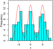
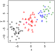
Figure 1: Left: the simulated data used to fit the toy model in Section 4.1. Center: histogram of the simulated covariates, along with the 3-Gaussian-mixture distribution from which they are drawn. Right: the simulated data, with colors/symbols reflecting the cluster assignments of the Dirichlet model at one step in the fit.

Suppose we had a physical basis for a 3-component model (or suspected 3 components, by inspection), but wanted to allow for the possibility of more or less structure than a strict Gaussian mixture provides. The Dirichlet process supplies a way to do this. For a given $\kappa$ and $n$, the distribution of $K$ is known, so in principle a prior expectation for the number of clusters, say $3\pm 1$, can be roughly translated into a Gamma prior on $\kappa$. Here I instead adopt an uninformative prior on $\kappa$ (Dorazio, 2009), and compare the results to those of a Gaussian mixture model with $K=3$.

Using the Dirichlet process model, results from a chain of 1000 Gibbs samples (discarding the first 10) are shown as shaded histograms in Figure 1. The results are consistent with the input model values (vertical, dashed lines) for the parameters of interest ($\alpha$, $\beta$ and $\Sigma$). The latent parameters describing the base distribution of the Dirichlet process are also consistent with the toy model, although they are poorly constrained. The right panel of Figure 1 shows the cluster assignments for a sample with $K=6$ (the median of the chain); the clustered nature of the data is recognized, although the number of clusters tends to exceed the number of components in the input model. An equivalent analysis using a mixture of 3 Gaussians rather than a Dirichlet process model produces very similar constraints on the parameters of interest (hatched histograms in Figure 2).

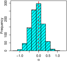
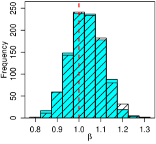
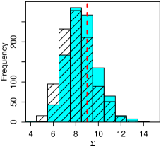
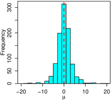
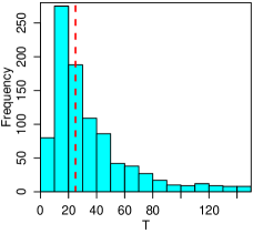
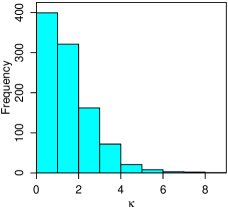
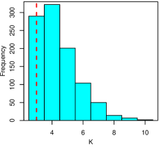
Figure 2: Histograms of parameter samples using a Dirichlet process (blue shaded) or 3-Gaussian mixture (hatched) prior on the distribution of covariates, for the toy-model analysis of Section 4.1. Dashed vertical lines indicate the input values used to generate the data set. The hyperparameters of the Gaussian mixture model are not shown; these correctly converge to the mean and width of the three mixture components.

4.2 Scaling relations of relaxed galaxy clusters

As a real-life astrophysical example, I consider the scaling relations of dynamically relaxed galaxy clusters, using measurements presented by Mantz et al. (2015). Note that there are a number of subtleties in the interpretation of these results that will be discussed elsewhere; here the problem is considered only as an application of the method presented in this work.

Briefly, the data set comprises X-ray measurements of 40 massive, relaxed clusters. The X-ray observables are total mass, $M$; gas mass, $M_{\mathrm{gas}}$; average gas temperature, $kT$; and luminosity, $L$. In addition, spectroscopically measured redshifts are available for each cluster. A simple model of cluster formation by spherical collapse under gravity, neglecting gas physics, predicts self-similar power-law scaling relations among these quantities:

$$M_{\mathrm{gas}} \propto M,$$ (63)

$$kT \propto \left[E(z)\,M\right]^{2/3},$$

$$L \propto E(z)^{1.92}\,M^{0.92},$$

where $E(z)=H(z)/H_{0}$ is the normalized Hubble parameter at the cluster’s redshift. The aim of this analysis is to test whether the power-law slopes above are accurate, and to characterize the joint intrinsic scatter of $M_{\mathrm{gas}}$, $kT$ and $L$ at fixed $M$ and $z$. Taking the logarithm of these physical quantities, and assuming log-normal measurement errors and intrinsic scatter, this becomes a linear regression with $p=2$ and $m=3$. For brevity, and neglecting units, $(\ln E,\ln M)\rightarrow(x_{1},x_{2})$ and $(\ln M_{\mathrm{gas}},\ln kT,\ln L)\rightarrow(y_{1},y_{2},y_{3})$; I also approximately center the covariates for convenience. Figure 3 shows summary plots of these data. Although measurement errors are shown as orthogonal bars for clarity, the analysis will use a full $5\times 5$ covariance matrix accounting for the interdependence of the X-ray measurements (this covariance is illustrated for one cluster in the figure).

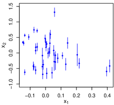
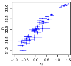
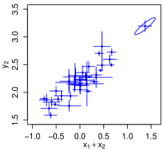
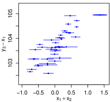
Figure 3: Scatter plots showing the distribution of measured covariates and responses for the $p=2$, $m=3$ problem of fitting galaxy cluster scaling relations described in Section 4.2. An ellipse illustrates the measurement covariance for the most massive (largest $x_{2}$) cluster in each panel. The particular combinations of $x$ and $y$ plotted are conventional (cf. Equation 63).

Because the redshifts are measured with very small uncertainties, this problem is not well suited to the Dirichlet process prior; intuitively, the number of clusters in the Dirichlet process must approach the number of data points because the data are strongly inconsistent with one another (i.e. are not exchangeable). Instead, I use a Gaussian mixture prior with $K=3$, and verify that in practice the results are not sensitive to $K$ (the parameters of interest differ negligibly from an analysis with $K=1$).

Marginalized 2-dimensional constraints on the power-law slopes of each scaling relation are shown in the top row of Figure 4 (68.3 and 95.4 per cent confidence). On inspection, only the luminosity scaling relation appears to be in any tension with the expectation in Equation 63, having a preference for a weaker dependence on $E(z)$ and a stronger dependence on $M$. These conclusions are in good agreement with a variety of earlier work (e.g. Reiprich & Böhringer 2002; Zhang et al. 2007, 2008; Mantz et al. 2010; Rykoff et al. 2008; Pratt et al. 2009; Vikhlinin et al. 2009; Leauthaud et al. 2010; Reichert et al. 2011; Sereno & Ettori 2015; see also the review of Giodini et al. 2013).

The posterior distributions of the elements of the multi-dimensional intrinsic covariance matrix are shown in the bottom row of Figure 4, after transforming to marginal scatter (square root of the diagonal) and correlation coefficients (for the off-diagonal elements). The intrinsic scatters of $M_{\mathrm{gas}}$ and $kT$ at fixed $M$ and $z$ are in good agreement with other measurements in the literature (see Allen et al. 2011; Giodini et al. 2013, and references therein); the scatter of $L$ is lower than the $\sim 40$ per cent typically found, likely because this analysis uses a special set of morphologically similar clusters rather than a more representative sample. The correlation coefficients are particularly challenging to measure, and the constraints are relatively poor. Nevertheless, the ability to efficiently place constraints on the full intrinsic covariance matrix is an important feature of this analysis. Within uncertainties, these results agree well with the few previous contraints on these correlation coefficients in the literature (Mantz et al., 2010; Maughan, 2014). The best-fitting intrinsic covariance matrix is illustrated visually in Figure 5, which compares it to the residuals of $\textstyle y$ with respect to the best-fitting values of $\textstyle x$ and the best-fitting scaling relations.

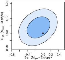
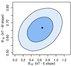
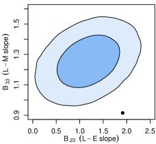
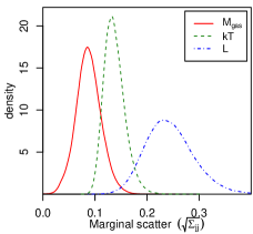
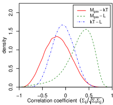
Figure 4: Top row: joint 68.3 and 95.4 per cent confidence regions on the slope parameters of each of the scaling relations in Equation 63. Black circles indicate the self-similar expectation given in Equation 63. Bottom left: posterior distributions for the marginal intrinsic scatter parameters of the model. Bottom right: posteriors for the off-diagonal intrinsic scatter terms, expressed as correlation coefficients.

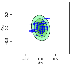
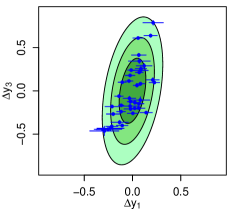
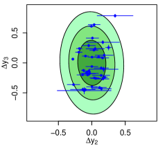
Figure 5: Residuals of $\textstyle y$ with respect to the best-fitting values of $\textstyle x$ and the best-fitting scaling relations. For clarity, measurement errors are shown as orthogonal bars, even though the measurement covariances are non-trivial. In particular, the “by-eye” positive correlation in the left panel is due to a positive correlation in the measurement uncertainties. Shaded ellipses correspond to 1, 2 and $3\sigma$ intrinsic scatter (in the 2 dimensions shown in each panel), according to the best-fitting intrinsic covariance matrix.

5 Summary

I have generalized the Bayesian linear regression method described by K07 to the case of multiple response variables, and included a Dirichlet process model of the distribution of covariates (equivalent to a Gaussian mixture whose complexity is learned from the data). The algorithm described here is implemented independently of the linmix_err IDL code of K07 as an r package called lrgs, which is publicly available. Two examples, respectively using a toy data set and real astrophysical data, are presented.

A number of further generalizations are possible. In principle, significant complexity can be added to the model of the intrinsic scatter in the form of a Gaussian mixture or Dirichlet process model (with a Gaussian base distribution) while maintaining conjugacy of the conditional posteriors, and thereby the efficiency of the Gibbs sampler. The case censored data (upper limits on some measured responses) is discussed by K07. This situation, or, more generally, non-Gaussian measurement errors, can be handled by rejection sampling (at the expense of efficiency) but is not yet implemented in lrgs. Also of interest is the case of truncated data, where the selection of the data set depends on one of the response variables, and the data are consequently an incomplete and biased subset of a larger population. This case can in principle be handled by modeling the selection function and imputing the missing data (Gelman et al., 2004). lrgs is shared publicly on GitHub, and I hope that users who want more functionality will be interested in helping develop the code further.

References

- Allen et al. (2011) Allen S. W., Evrard A. E., Mantz A. B., 2011, ARA&A, 49, 409
- Antoniak (1974) Antoniak C. E., 1974, The Annals of Statistics, 2, 1152
- Barnard et al. (2000) Barnard J., McCulloch R., Meng X.-L., 2000, Statistica Sinica, 10, 1281
- Dorazio (2009) Dorazio R. M., 2009, Journal of Statistical Planning and Inference, 139, 3384
- Escobar & West (1995) Escobar M. D., West M., 1995, Journal of the American Statistical Association, 90, 577
- Gelman et al. (2004) Gelman A., Carlin J. B., Stern H. S., Rubin D. B., 2004, Bayesian Data Analysis. Chapman & Hall/CRC
- Giodini et al. (2013) Giodini S., Lovisari L., Pointecouteau E., Ettori S., Reiprich T. H., Hoekstra H., 2013, Space Sci. Rev., 177, 247
- Kelly (2007) Kelly B. C., 2007, ApJ, 665, 1489
- Leauthaud et al. (2010) Leauthaud A. et al., 2010, ApJ, 709, 97
- Mantz et al. (2010) Mantz A., Allen S. W., Ebeling H., Rapetti D., Drlica-Wagner A., 2010, MNRAS, 406, 1773
- Mantz et al. (2015) Mantz A. B., Allen S. W., Morris R. G., Schmidt R. W., 2016, MNRAS, 456, 4020
- Maughan (2014) Maughan B. J., 2014, MNRAS, 437, 1171
- Murugiah & Sweeting (2012) Murugiah S., Sweeting T., 2012, Journal of Statistical Planning and Inference, 142, 1947
- Neal (2000) Neal R. M., 2000, Journal of Computational and Graphical Statistics, 9, 249
- O’Malley & Zaslavsky (2008) O’Malley A. J., Zaslavsky A. M., 2008, Journal of the American Statistical Association, 103, 1405
- Pratt et al. (2009) Pratt G. W., Croston J. H., Arnaud M., Böhringer H., 2009, A&A, 498, 361
- Reichert et al. (2011) Reichert A., Böhringer H., Fassbender R., Mühlegger M., 2011, A&A, 535, A4
- Reiprich & Böhringer (2002) Reiprich T. H., Böhringer H., 2002, ApJ, 567, 716
- Robotham & Obreschkow (2015) Robotham A. S. G., Obreschkow D., 2015, PASA, 32, e033
- Rykoff et al. (2008) Rykoff E. S. et al., 2008, MNRAS, 387, L28
- Schneider et al. (2015) Schneider M. D., Hogg D. W., Marshall P. J., Dawson W. A., Meyers J., Bard D. J., Lang D., 2015, ApJ, 807, 87
- Sereno & Ettori (2015) Sereno M., Ettori S., 2015, MNRAS, 450, 3675
- Vikhlinin et al. (2009) Vikhlinin A. et al., 2009, ApJ, 692, 1033
- Zhang et al. (2007) Zhang Y.-Y., Finoguenov A., Böhringer H., Kneib J.-P., Smith G. P., Czoske O., Soucail G., 2007, A&A, 467, 437
- Zhang et al. (2008) Zhang Y.-Y., Finoguenov A., Böhringer H., Kneib J.-P., Smith G. P., Kneissl R., Okabe N., Dahle H., 2008, A&A, 482, 451