Assessing Galaxy Limiting Magnitudes in Large Optical Surveys

Abstract

Large scale structure measurements require accurate and precise knowledge of the survey depth — typically expressed in the form of a limiting magnitude — as a function of position on the sky. To date, most surveys only compute the point-source limiting magnitude measured within a fixed metric aperture. However, this quantity is ill suited to describe the limiting depth of galaxies, which depends on the detailed interplay of survey systematics with galaxy shapes and sizes. We describe an empirical method for directly estimating the limiting magnitude for large photometric surveys, and apply it to $\sim 10,000\,\mathrm{deg}^{2}$ of SDSS DR8 data. Combined with deeper imaging from SDSS Stripe 82 and CFHTLens, we are able to use these depth maps to estimate the location-dependent galaxy detection completeness at any point within the full BOSS DR8 survey region. We show that these maps can be used to construct random points suitable for unbiased estimation of correlation functions for galaxies near the survey limiting magnitude. Finally, we provide limiting magnitude maps for galaxies in SDSS DR8 in HEALPix format with NSIDE=2048.

1. Introduction

In recent years, observational astronomy has been revolutionized by wide-field optical surveys. The impact of the data from the Sloan Digital Sky Survey (SDSS York et al. 2000) has been enormous, covering a range of topics too broad to mention. The next era of large photometric surveys is now upon us, with the Dark Energy Survey (DES The DES Collaboration 2005) underway, imaging 5,000 deg² with a depth that is two magnitudes deeper than that of SDSS. Similar surveys like the Kilo-Degree Survey (KiDS de Jong et al. 2015) and the Hyper-Suprime Camera (HSC) are also underway. By the end of the decade the Large Synoptic Survey Telescope (LSST Ivezic et al. 2008) will start to take data, with unprecedented depth over fully half the sky. However, as hard as we try to build homogeneous surveys with uniform depth, there will always be variations in sky coverage, with exposure time, seeing, sky brightness, and other factors varying over the course of nights and seasons. These systematic variations can impact the scientific products derived from these surveys, affecting spectroscopic target selection, optical cluster measurements, and correlation function measurements (to name but a few).

One obvious option to mitigate these factors is to limit any object selection to those regions where the imaging is nearly complete. This of course raise the question of choosing which regions have high completeness. One option is to mask out regions which have anomalously low object density (e.g. Liu et al. 2015). Other options include cross-correlating galaxy densities with known sources of systematic errors in order to choose which regions were contaminated and should be masked, as for early studies with SDSS (Scranton et al. 2002). The Baryon Oscillation Spectroscopic Survey (BOSS Schlegel et al. 2009) made use of relatively faint targets, requiring more sophisticated analyses (Ross et al. 2011). Galaxy detection probabilities were estimated via cross-correlation with systematics maps, and galaxies used in the correlation function measurements were reweighted accordingly. However, these effects were mostly perturbative for the spectroscopic targets considered.

The WiggleZ spectroscopic survey (Blake et al. 2010) had a much more challenging task due to the combination of SDSS and Galaxy Evolution Explorer (GALEX) target selection. Density variations as a function of Galactic dust and GALEX exposure time were modeled via a simple completeness function. These models were then used to compute the full survey selection function. Most recently, a significant amount of effort has gone into simulating the selection function directly over a large survey by inserting and measuring fake galaxies with known properties (i.e. the Balrog code, Suchyta et al. 2015). Although this may be the most robust method, it suffers from a couple limitations. First, it can be expensive. Second, inserting fake galaxies will tend to correlate existing structure with the selection function, somewhat muddying the interpretation of the resulting random catalogs. Of course, this effect is in the real data as well, but since the interpretations are non-trivial, having a completely independent approach for characterizing selection functions can be highly complementary.

In this paper, we suggest an alternative, pragmatic approach. The main idea behind our measurement is simple: the magnitude error $\Delta m$ of a galaxy should be a function of the galaxy’s magnitude and the survey depth: the deeper the survey, the smaller the photometric error $\sigma_{m}$. Given a model for magnitude errors as a function of magnitude and survey depth $\sigma_{m}=g(m|m_{\mathrm{lim}})$, we use observations of galaxies $(m,\Delta m)$ over a patch of sky to recover the limiting magnitude $m_{\mathrm{lim}}$ of the survey patch. In practice, this direct measurement of the survey depth can only be done in relatively coarse pixels. We overcome this difficulty by fitting the recovered depth map as a function of the systematics map for the survey (e.g. sky noise, PSF size, etc), and then utilize these fine structure maps to generate a final high resolution estimate of the survey depth.

The layout of this paper is as follows. In Section 2 we describe the SDSS data used in this paper, although our method is fully generalizable to any survey data. In Section 3 we describe our method for measuring the survey depth in coarse pixels on the sky, and in Section 4 we show how we can use machine learning methods to reconstruct the survey depth at high resolution by making use of detailed maps of survey systematics. In Section 5, we use deeper data to model the galaxy detection completeness, and show how this is a simple function of survey depth. In Section 6 we show a practical application of our method in a simulated computation of the correlation function near the survey limiting magnitude where depth and completeness variations are significant. Finally, in Section 7 we summarize our findings.

2. Data

As discussed above, our method is designed to handle an arbitrary photometric galaxy catalog. As a case study, in this paper we determine the depth of SDSS DR8 photometric data.

2.1. SDSS DR8 Photometry

The input galaxy catalog for this work is derived from SDSS DR8 data (Aihara et al. 2011). This data release includes more than $14,000\,\mathrm{deg}^{2}$ of drift-scan imaging in the Northern and Southern Galactic caps. The survey edge used is the same as that used for BOSS target selection (Dawson et al. 2013), which reduces the total area to $\approx 10,500\ \deg^{2}$ with high-quality observations and a well-defined contiguous footprint.

The galaxy selection employed is nearly the same as that used in the construction of the SDSS DR8 redMaPPer cluster catalog (Rykoff et al. 2014). The primary difference is that we limit the catalog to $i_{\mathrm{cmod}}<22.0$, rather than $i_{\mathrm{cmod}}<21$, to ensure that we have galaxies that are fainter than the $10\sigma$ limiting magnitude over the full survey footprint. Furthermore, we have not corrected for Galactic reddening. We then filter all objects with any of the following flags set in the $g$, $r$, or $i$ bands: SATUR_CENTER, BRIGHT, TOO_MANY_PEAKS, and (NOT BLENDED OR NODEBLEND).

In this work, we reconstruct the SDSS DR8 MODEL_MAG limiting magnitudes in $u$, $g$, $r$, $i$ and $z$, and the composite CMODEL_MAG limiting magnitudes in $r$ and $i$. The MODEL magnitudes are estimated by fitting each of an exponential and deVaucouleurs profile to each galaxy in the $r$ band, and applying the better-fit model to each individual band. As such, MODEL magnitudes are suitable for galaxy color measurements. The composite CMODEL magnitudes are computed as a linear combination of the best-fit exponential and deVaucouleurs models, and are useful for galaxy total magnitude measurements. In this paper, we denote MODEL and CMODEL magnitudes with subscripts “mod” and “cmod” respectively.

2.2. SDSS Systematics Maps

The SDSS survey consists of drift-scan imaging of a large number of stripes that extend along great circles (York et al. 2000). Because of the CCD layout, each stripe is scanned at least twice, with six interleaving camera columns. These two scans may have different seeing and sky noise parameters, yielding the possibility of a “cat scratch” pattern of imaging systematics. The SDSS imaging pipeline divides each camera column into “fields”, which are rectangular patches of size $~{}145\,\mathrm{arcmin}^{2}$. Due to the interleaving nature of the scanning survey, there are overlaps between neighboring fields.

For SDSS DR8, to create a uniform single-pass survey and resolve field overlaps, each field is given a score based on the $r$-band seeing, the sky brightness in $r$, and an estimate of photometricity of the night (Aihara et al. 2011). Fields with higher scores are determined to be “primary”, with an additional percolation step that tries to keep regions as homogeneous as possible. However, as shown below there can still be a large variation in systematics over small scales at the edges of stripes and camera columns.

At the end of this procedure, each point on the sky is associated with a single primary field. The primary window function thus determined is available from the SDSS-III website. To implement the window function, the sky is broken into many mangle polygons (Swanson et al. 2008), each of which is linked to a primary field. In this way each point in the survey can be uniquely associated with a point spread function (PSF) full width half maximum (FWHM), sky level, and sky noise in all five bands. In addition, the observation time can be used to compute the airmass (D. Schlegel, private communication).

For the analysis in this paper, we have converted the window function into HEALPix maps with NSIDE=2048. Each pixel has a size of $2.95\,\mathrm{arcmin}^{2}$, which is of sufficiently high resolution to capture the fine scale variations of the systematics maps. However, for pixel-level precision then the full mangle polygon description of the window function should be used.

3. Measuring Survey Depth

3.1. Relating Survey Photometry to Survey Depth

Let $m_{\mathrm{gal}}$ be the magnitude of a galaxy. If $F$ is the flux of a source in units of nanomaggies, the flux is related to galaxy magnitude via

$$F=10^{-0.4(m_{\mathrm{gal}}-m_{\mathrm{ZP}})}.$$ (1)

where $m_{\mathrm{ZP}}=22.5$. If $S$ is the number of signal photons reaching the detector, one has that the expectation value for $S$ is related to the galaxy flux via

$$\langle{S}\rangle=kt_{\mathrm{eff}}F$$ (2)

where $k$ is a proportionality constant, and $t_{\mathrm{eff}}$ is the effective exposure time. The corresponding number of noise-photons $N$ is

$$\langle{N}\rangle=kt_{\mathrm{eff}}F_{\mathrm{noise}}$$ (3)

where $F_{\mathrm{noise}}$ is the effective noise flux. The noise flux can have multiple origins, e.g. sky, read noise, etc. Here, we have lumped any such contributions into a single term. Given $N$ signal photons, an unbiased estimate for the galaxy flux is

$$\hat{F}=\frac{S+N}{kt_{\mathrm{eff}}}-F_{\mathrm{noise}}.$$ (4)

Since both $S$ and $N$ follow Poisson statistics, the variance in $\hat{F}$ is

$$\sigma_{F}^{2}=\frac{\langle{S}\rangle+\langle{N}\rangle}{k^{2}t_{\mathrm{eff}}^{2}}=\frac{F+F_{\mathrm{noise}}}{kt_{\mathrm{eff}}}$$ (5)

The corresponding magnitude error is

$$\begin{split}\sigma_{m}(F;F_{\mathrm{noise}},t_{\mathrm{eff}})&=\frac{2.5}{\ln 10}\frac{\sigma_{F}}{F}\\ &=\frac{2.5}{\ln 10}\left[\frac{1}{Fkt_{\mathrm{eff}}}\left(1+\frac{F_{\mathrm{noise}}}{F}\right)\right]^{1/2}\end{split}$$ (6)

The above expression relates the flux of a galaxy to its corresponding magnitude error. In practice, we recast $F_{\mathrm{noise}}$ in terms of the $10\sigma$ limiting flux $F_{\mathrm{lim}}$ defined via $F_{\mathrm{lim}}/\sigma_{F}=10$. Solving for $F_{\mathrm{noise}}$, we have

$$F_{\mathrm{noise}}=\frac{F_{\mathrm{lim}}^{2}kt_{\mathrm{eff}}}{10^{2}}-F_{\mathrm{lim}}$$ (7)

The limiting magnitude $m_{\mathrm{lim}}$ is simply the magnitude associated with a galaxy of flux $F_{\mathrm{lim}}$.

Equations 1, 6 and 7 together define our model for the magnitude error $\sigma_{m}(m;m_{\mathrm{lim}},t_{\mathrm{eff}})$ of a galaxy of magnitude $m$ in a survey patch of limiting magnitude $m_{\mathrm{lim}}$ and effective exposure time $t_{\mathrm{eff}}$. Note that in practice, the effective time $t_{\mathrm{eff}}$ is always accompanied by the normalization constant $k$, which can be absorbed into the definition of the parameter $t_{\mathrm{eff}}$.

A note on dust and dereddened magnitudes: Note that in the above derivation, the relevant quantity is the observed magnitude $m$, or the observed flux $F$. Whether the flux has been attenuated due to dust or not is completely irrelevant; the only thing that matters is the total arriving flux. Consequently, one should not use dereddened magnitudes when estimating the limiting magnitude of a survey.

Conversely, we emphasize that the limiting magnitude we recover is a property of the survey. To relate our measured limiting magnitude to a dereddened limiting magnitude, one must apply the necessary reddening corrections. As part of the data release associated with this paper, for convenience we include the necessary dust maps in the equatorial coordinate system that we use. We have chosen not to apply these maps to allow for the use of different Galactic dust models.

3.2. Computing the Depth Maps

As a practical application, we fit our model to SDSS DR8 data. Specifically, given a patch of sky, we fit our model of magnitude errors to the reported magnitude errors so as to derive the effective limiting magnitude and exposure times. In this procedure, we assume that the errors as quoted are correct. Observationally, while we have magnitude error estimates, we do not have “errors on the error”, so it is not obvious how to best fit the observational data to our model. In order to minimize the impact of gross outliers, we have chosen to fit our model by minimizing the total absolute deviation from the model, i.e. we minimize the cost function

$$E(m_{\mathrm{lim}},t_{\mathrm{eff}})=\sum_{\alpha}\left|\sigma_{m}^{\mathrm{obs}}-\sigma_{m}(m_{\alpha}|m_{\mathrm{lim}},t_{\mathrm{eff}})\right|$$ (8)

where the sum is over all galaxies within a given sky patch. The function is minimized using the downhill-simplex method of Nelder & Mead (1965) as implemented in the IDL AMOEBA function, and errors on the parameters are derived by bootstrap resampling the galaxies 50 times and refitting.

Figure 1 illustrates this technique for a single HEALPix pixel of NSIDE=256 in DR8. We fit all galaxies with signal-to-noise (S/N) greater than $5$ in the pixel, which is deep enough to get a good measurement of the $10\sigma$ magnitude limit, but shallow enough to ensure that the SDSS “luptitudes” (arcsinh magnitudes) are equivalent to logarithmic magnitudes. In all panels in the figure, red dashed lines are our model fit. The black dotted lines show our recovered $10\sigma$ limiting magnitude.

Figure 1.— Magnitude error vs. magnitude for three magnitude definitions in a single HEALPix pixel of NSIDE=256, as follows: (a) SDSS FIBER2MAG, an aperture magnitude of diameter 2″. (b) Same as above for MODEL_MAG. (c) Same as above for CMODEL_MAG. Red dashed lines show our model fits, and black dotted lines mark the recovered $10\sigma$ limiting magnitude. Note our model provides an excellent description of the noise for fixed metric aperture magnitudes, while model fitting magnitudes result in noisier fits due to variations introduced by galaxy size. The outlier points in the top panel are from regions that have a different local depth in our relatively large pixel.

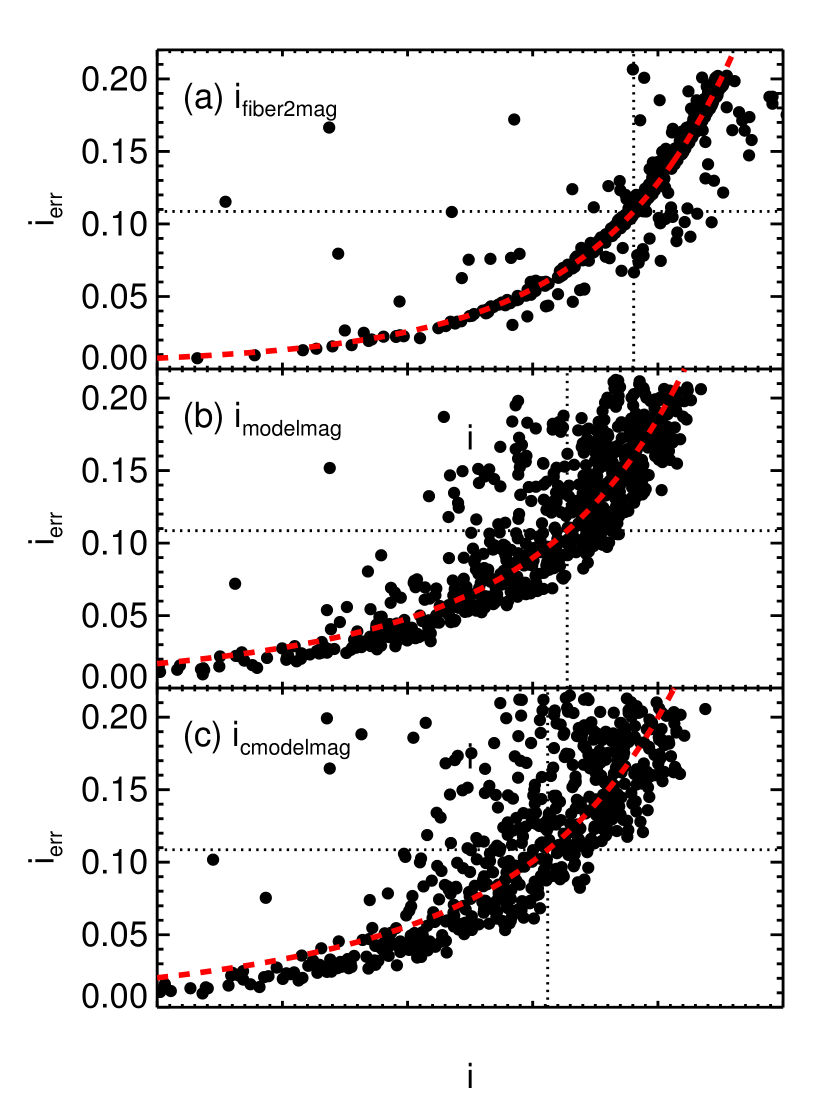
The different panels corresponds to different magnitude definitions. The top panel uses SDSS FIBER2MAG, an aperture magnitude of diameter 2″. We see that in this case the model provides an excellent description of the data, as we would expect. The outlier points are from regions that have a different local depth than the bulk of the relatively large pixel. Section 4 demonstrates how we deal with this issue in our final depth map estimates. The middle and lower panels show the $i$-band MODEL and CMODEL magnitudes, which are derived from model fits to the galaxy data. We see that in this case there is significant scatter due to the fact that the photometric noise for these model-fit apertures must necessarily depend on additional variables such as galaxy size. Nevertheless, it is clear that our model still provides a reasonable description of the relation between galaxy magnitude and magnitude error, especially at the faint end where we are trying to estimate the limiting magnitude.

In order to achieve a reliable fit of $m_{\mathrm{err}}$ vs. $m_{\mathrm{gal}}$, we find we require at least 100 galaxies with signal-to-noise greater than $5$. At the typical limiting magnitude of the SDSS survey, this is achieved by pixelizing the sky with HEALPix NSIDE=256, or $190\,\mathrm{arcmin}^{2}$ per pixel. Note this is significantly coarser than the variations of the systematics maps, which introduces some noise to our fits which we will quantify in Section 4.4. In some cases, especially at the survey edges and for most of the survey in the much shallower $u$ band, there are insufficient galaxies to perform the fit with NSIDE=256. When this happens we expand to the next coarsest pixelization (NSIDE=128), and if this still does not yield enough galaxies we use NSIDE=64.

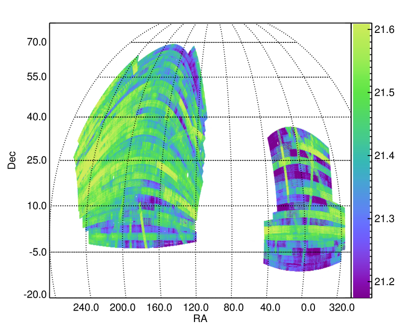
Figure 2 shows the measured depth map for $r_{\mathrm{cmod}}$. There is significant structure on all scales, with an amplitude of $0.5\,\mathrm{mag}$. There are several striking features in the map. First, the stripe scanning pattern is immediately apparent, as are the “cat scratch” features from interleaving camera columns taken under different conditions. Second, when the perpendicular “übercal” stripes were taken under favorable conditions, these were chosen as primary fields, and thus are significantly deeper. Third, the northern Galactic cap (NGP) region is typically deeper than the southern Galactic cap (SGP) region. The obvious exception is Stripe 82 in the south. This region was scanned multiple times, and thus only the best observations were determined to be primary fields for DR8.

Figure 2.— Depth map for $r_{\mathrm{cmod}}$. The amplitude of the depth variations is $0.5\,\mathrm{mag}$, which will be larger after correcting for Galactic reddening. There are numerous features that are described in the text in Section 3.2.

After performing the two-parameter fit to each of the pixels independently, we note that the $t_{\mathrm{eff}}$ and $m_{\mathrm{lim}}$ parameters are highly correlated. This is illustrated in Figure 3 where we show a sample of pixels for both $r_{\mathrm{mod}}$ and $i_{\mathrm{mod}}$. We fit a linear model

$$\ln t_{\mathrm{eff}}=a+b(m_{\mathrm{lim}}-21.0),$$ (9)

where 21.0 is a convenient pivot point. The residual scatter from the model in both cases is $\sim 20\%$.

Figure 3.— $t_{\mathrm{eff}}$ vs. $m_{\mathrm{lim}}$ for (a) $r_{\mathrm{mod}}$ and (b) $i_{\mathrm{mod}}$, shown for a sample of pixels for clarity. Red dashed line shows a least-absolute-deviation fit. The residual scatter is $\sim 20\%$.

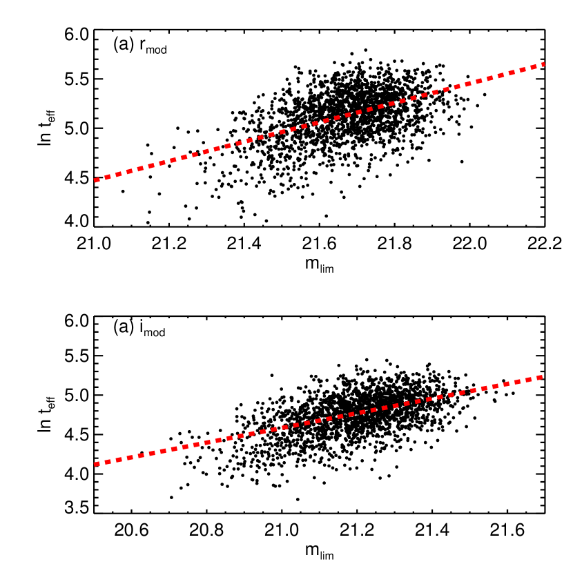
In light of the correlation between limiting magnitude and survey depth, we have chosen to characterize the survey depth with the single quantity $m_{\mathrm{lim}}$ (the more relevant quantity), setting the effective exposure time via equation 9. Table 1 shows the fit parameters for the magnitudes used in this paper. The efficacy of this approximation is tested in the next section.

Table 1$t_{\mathrm{eff}}$ vs. $m_{\mathrm{lim}}$ Fit Parameters

Magnitude	$a$	$b$
$u_{\mathrm{mod}}$	3.41	1.15
$g_{\mathrm{mod}}$	4.27	0.85
$r_{\mathrm{mod}}$	4.53	0.91
$i_{\mathrm{mod}}$	4.56	1.00
$z_{\mathrm{mod}}$	4.39	1.34
$r_{\mathrm{cmod}}$	4.34	1.70
$i_{\mathrm{cmod}}$	4.48	1.23

Note. — $t_{\mathrm{eff}}=\exp[a+b(m_{\mathrm{lim}}-21.0)]$

4. Reconstruction of the Depth Maps

4.1. Introduction to the Problem

In principle, Figure 2 is exactly what we are looking for: a map of the limiting magnitude of the survey everywhere in the sky. In practice, however, our measurement is severely limited by the need to have $\sim 100$ galaxies in a sky pixel in order to perform our measurement. This limitation renders the pixels so wide that important features in the small scale structure of the survey are missed.

To overcome this difficulty, we rely on the fact that the observed depth map is a natural consequence of the survey observing conditions. For instance, better seeing conditions leads to deeper data. The fundamental insight is that the limiting magnitude $m_{\mathrm{lim}}(\bm{\hat{n}})$ at a position angle $\bm{\hat{n}}$ is a function of systematic parameters such as sky noise, seeing, etc. Let then $\bm{p}(\bm{\hat{n}})$ be the vector that collects all systematics parameters at position $\bm{\hat{n}}$. We posit that the function $m_{\mathrm{lim}}(\bm{\hat{n}})$ takes the form

$$m_{\mathrm{lim}}(\bm{\hat{n}})=f(\bm{p}(\bm{\hat{n}}))$$ (10)

where $f$ is some unknown function. We seek to estimate the function $f$ given a series of inputs $\bm{p}(\bm{\hat{n}})$ — the systematics evaluated for each of our coarse pixels — and a series of outputs $m_{\mathrm{lim}}$ — our measured depth. This is a problem that is well suited to machine learning methods. Here, we rely on the Random Forest (RF) technique (Breiman 2001), as implemented in the python module sklearn.

4.2. Method

The first step is to decide which set of systematics maps will be used to train the RF method. We have opted for an inclusive approach, and attempted to utilize all the systematic information that may be relevant. This includes the PSF FWHM, sky level, and sky sigma for the band being fit; the airmass; and the value of the $E(B-V)$ map from Schlegel et al. (1998). Although we do not expect the depth to depend on $E(B-V)$ directly, there may be some second-order correlations. As the model magnitude depends on the galaxy model as fit in the $r$-band, we additionally include the $r$-band systematics maps (PSF FWHM, sky, and sky sigma) in each of the fits. Furthermore, the drift-scan method of SDSS has all the bands observed at roughly the same time, so the seeing and sky in the various bands are correlated and thus we can beat down the noise by using measurements from different bands. For this reason, when we fit the $r$-band depth we additionally include the $i$-band systematics maps in the fit.

When training the RF, it is critical that the systematics information be appropriately handled. Specifically, because our observed depth is measured over coarse angular pixels, the high resolution systematics maps must be averaged to the same coarser resolution employed in our measurements prior to training the RF. To perform this “de-resolution” we start with the coarse target NSIDE=256 map. In the HEALPix nested scheme it is then trivial to find all the subpixels at NSIDE=2048 for each of the coarse pixels. We then take the average of the systematics value in the subpixels that are within the SDSS footprint, as well as tracking the fraction of subpixels that are outside the footprint.

Having averaged our systematics map, we train the RF. In each run, we use half the pixels for training and half for validation. In all cases, we only use coarse pixels that have at least 80% of the subpixels in the footprint to avoid problems at the boundaries. We have also run checks where we train on points co-located on the sky to ensure that the classifier is not unintentionally picking up on position information encoded in nearby correlated pixels, and have achieved similar performance. However, in the case where we train on the NGP region and apply to the SGP region (and vice versa) the resulting performance is degraded. This hints at some subtle differences in the systematics properties of the north and south of the SDSS region.

Finally, having trained the RF to calibrate the function $m_{\mathrm{lim}}=f(\bm{p})$ using our low resolution systematics map, we apply the RF on the high resolution maps so as to recover a high resolution map of the limiting magnitude $m_{\mathrm{lim}}(\bm{\hat{n}})$.

4.3. Results

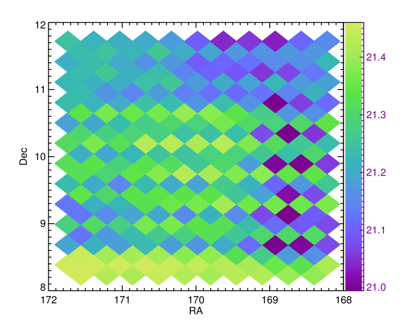
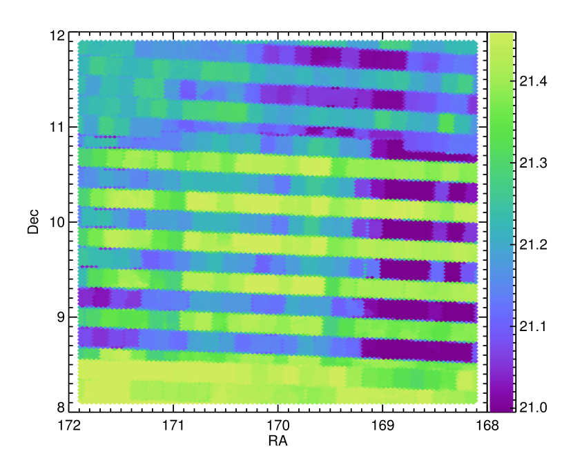
Figure 4 illustrates the fundamental result from our analysis: a high resolution reconstructed map of the limiting magnitude $m_{\mathrm{lim}}(\bm{\hat{n}})$. For plotting purposes, the map was averaged to NSIDE=256. The structure of the map is very similar to the measured map in Figure 2. Figure 5 highlights the importance of our reconstruction procedure. The left panel shows a zoomed-in patch of $16\,\mathrm{deg}^{2}$ for the low resolution depth map with $\sim 200$ galaxies per pixel. While there is a noticeable gradient across this patch, no higher order structure is visible. The right panel shows the high resolution reconstructed depth map for the same patch. This exhibits the characteristic “cat scratch” structure inherent to the interleaved scanning utilized in SDSS. These depth variations are tracked by the high resolution systematics maps, and are recovered by our reconstruction procedure.

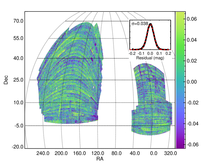
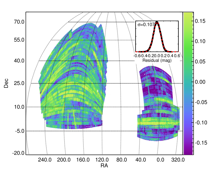
Figure 6 shows the residual between our observed limiting magnitude map, i.e., Figure 2, and our low resolution reconstructed map. As shown in the histogram in the inset plot, the RMS of the residuals is $\sigma_{\mathrm{resid}}=0.038\,\mathrm{mag}$ (for details on how this was computed, see Section 4.4). However, there is still some structure in the residuals that are visible at a low level. As we will show in Section 4.4, much of this residual is an artifact of the interplay of rapidly varying systematics maps and our averaging procedure.

Figure 4.— Reconstructed map of $r_{\mathrm{cmod}}$ depth using RF. The map was reconstructed at high resolution (HEALPix NSIDE=2048) and then averaged to NSIDE=256 as described in Section 4.2 for plotting and comparison to the measured map.

Figure 5.— Zoom in of $16\,\mathrm{deg}^{2}$ of depth map. Left: Low resolution (NSIDE=256) with $\sim 200$ galaxies per pixel used for the depth estimation. There is a noticeable gradient, but no higher order structure is visible. Right: High resolution (NSIDE=2048) reconstructed depth map showing the “cat scratches” characteristic of the interleaved scanning. These depth variations are tracked by the high resolution systematics maps, and are recovered by our reconstruction procedure.

Figure 6.— Residuals of reconstructed $r_{\mathrm{cmod}}$ depth compared to the observed limiting magnitude map. The histogram in the inset plot shows the RMS of the residuals, with a Gaussian fit (red) with $\sigma_{\mathrm{resid}}=0.038\,\mathrm{mag}$. There is some structure in the residuals that are visible at a low level. As shown in Section 4.4, the large outliers are caused by the averaging process used to compare the maps, but are not present in the underlying high resolution map.

4.4. Estimating Noise

We must now estimate the noise in the reconstructed depth maps. The most obvious estimate is the width of the residual distribution between the measured depth map and the reconstructed map as plotted in Figure 6. However, this estimate suffers from some limitations. Most importantly, our depth map has been measured at a relatively coarse scale (NSIDE=256), while the aim of our procedure is to reconstruct the map at a fine scale (NSIDE=2048). As the averaging procedure adds noise, this will inevitably overestimate the noise in the residual map as well as introduce spurious structures at field boundaries where the systematics vary rapidly.

As an alternative, we use a Monte Carlo technique to simulate data with known systematics and repeat our entire analysis procedure. A comparison of the true survey depth map used in the Monte Carlo to the recovered survey depth map will allow us to estimate the noise in the reconstructed maps. For our Monte Carlo simulation, we define the survey depth to be our estimated high resolution survey depth map, and for our input galaxy catalog we use the SDSS galaxy catalog, defining the observed magnitudes as truth for the Monte Carlo simulation. Our procedure is as follows:

1. Take the existing galaxy catalog, and set each (observed) magnitude as the “true” magnitude in each band.

2. Take the high resolution reconstructed depth map for each band as the “true” limiting magnitude (and associated $t_{\mathrm{eff}}$) at every point in the survey.

3. Given the true magnitude, $m_{\mathrm{lim}}$, and $t_{\mathrm{eff}}$, compute the associated magnitude error from Eqn. 6. Perturb the true magnitude according to this error.

4. Compute the depth map with NSIDE=256 as described in Section 3.2.

5. Refit the depth map and reconstruct a simulated high resolution depth map as described in Section 4.

In the end, we have a high resolution reconstructed depth map which can be directly compared to the “true” input map.

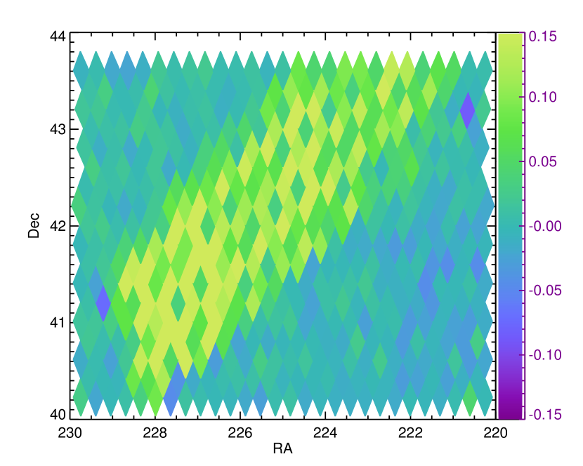
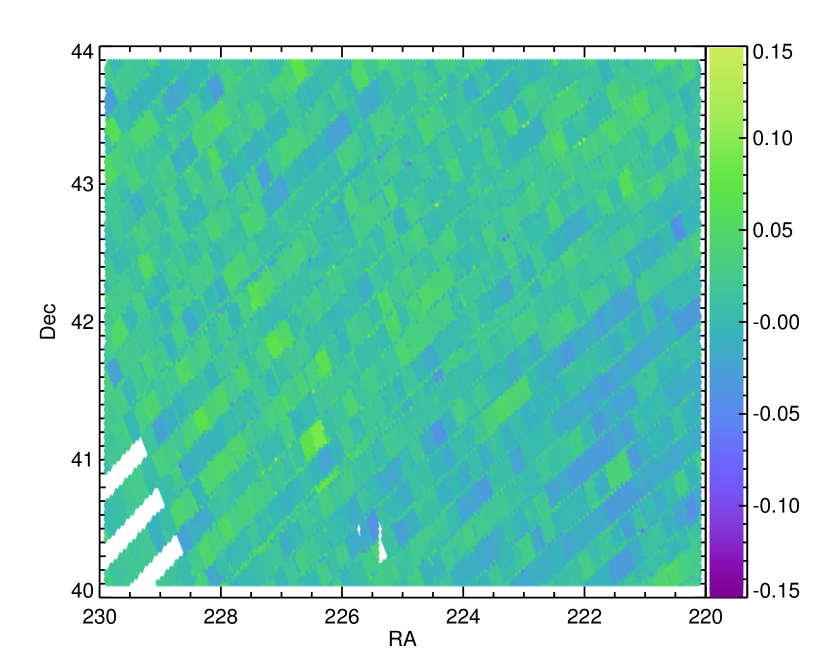
We find that the residual map between the raw measured depth map and our recovered high resolution depth map (degraded to the resolution of the measured map) has a striking similarity to that of Figure 6. Since we now have the high resolution “truth” in hand, we can determine the origin of the structures shown in Figure 6. Figure 7 shows a particularly problematic patch at $RA=225^{\circ}$, $DEC=42^{\circ}$. The left panel shows the NSIDE=256 residuals between the measured depth map and the averaged reconstructed map for the simulated data. The red streak shows a large offset of $>0.1\,\mathrm{mag}$, very similar to that observed in Figure 6 for the real data. The right panel shows the NSIDE=2048 high resolution residuals between the reconstructed simulated depth map and the “true” map used as an input. We see that the pattern essentially disappears. Evidently, the regions with large coherent residuals observed in Figure 6 are artifacts of the averaging process. Most importantly, our high resolution maps are successfully recovering high resolution features that are completely unresolved in the observed depth maps.

Figure 7.— Zoom in of simulated depth map residuals. Left: Low resolution (NSIDE=256) residuals between measured depth map and averaged reconstructed depth map for the simulated data. The red streak shows a large offset, similar to that of Figure 6. Right: High resolution (NSIDE=2048) residuals. The large offset is no longer present, highlighting that our procedure is recovering the limiting magnitude at fine scales.

In Table 2, we summarize the noise estimates for the reconstructed depth maps for two different methods. The first, $\sigma_{\mathrm{resid}}$, measures the width of the residual distribution between the measured depth map and the averaged reconstructed depth map (NSIDE=256), as in the inset plot of Figure 6. The second, $\sigma_{\mathrm{sim}}$, is the width of the residual distribution between the simulated reconstructed depth map and the “true” depth map. In all cases the width is estimated using the robust Gaussian histogram-fitting code histogauss.pro from the IDL Astronomy Library. Due to the fact that our simulated data cannot take into account all the various sources of unmodeled systematics, we consider $\sigma_{\mathrm{sim}}$ and $\sigma_{\mathrm{resid}}$ to be lower and upper bounds on the true noise of the reconstructed depth map.

Table 2Observed and Simulated Scatter

Magnitude	$\sigma_{\mathrm{resid}}$	$\sigma_{\mathrm{sim}}$
$u_{\mathrm{mod}}$	0.128	0.068
$g_{\mathrm{mod}}$	0.038	0.020
$r_{\mathrm{mod}}$	0.036	0.018
$i_{\mathrm{mod}}$	0.040	0.020
$z_{\mathrm{mod}}$	0.063	0.034
$r_{\mathrm{cmod}}$	0.038	0.018
$i_{\mathrm{cmod}}$	0.051	0.023

4.5. Using $5\sigma$ Point-Source Depth

Many sky surveys state depth in terms of $5\sigma$ point-source depth, and this is typically used for telescope exposure-time calculators. This has the advantage of being relatively straightforward to compute, but as we show in this section this does not scale trivially to the galaxy limiting magnitude which we are interested in computing.

The BOSS survey have independently modeled the $5\sigma$ point-source depth based on the formal errors from PSF photometry on stellar sources (D. Schlegel, private communication). BOSS uses a simple model of seeing, sky brightness, and airmass:

$$F(5\sigma)=a_{i}f_{i}\sqrt{s_{i}}10^{0.4k_{i}m_{i}},$$ (11)

where $f_{i}$ is the FWHM, $s_{i}$ is the sky flux, and $m_{i}$ is the airmass. The normalization term $a=\{0.387,0.218,0.241,0.297,0.665\}$ and the airmass term $k=\{0.49,0.17,0.10,0.06,0.06\}$ for bands $i=\{u,g,r,i,z\}$ respectively. This formula predicts the $5\sigma$ point-source depth to an accuracy of 12%, 4%, 4%, 5%, and 7%, nominally comparable to the accuracy of the galaxy depth reconstruction in this work, but for a different type of object.

To compare to the galaxy depth, we calculate the $5\sigma$ point-source depth at high resolution and then average the map to NSIDE=256 as above. We then apply a constant offset to account for the fact that the $10\sigma$ galaxy depth is considerably shallower than that for these point sources. In the case of $r_{\mathrm{cmod}}$, this offset is $1.43\,\mathrm{mag}$. Figure 8 shows the residual between our observed limiting magnitude map (Figure 2) and the low resolution map reconstructed from the point source depth. The RMS scatter is $11\%$, a factor of three larger than seen for our galaxy depth reconstruction technique in this paper. More importantly, there is significant structure in the residuals. In Section 6 we show the impact on correlation function measurements of using this map instead of a galaxy-appropriate map.

Figure 8.— Residuals of reconstructed $r_{\mathrm{cmod}}$ depth using the formula for the $5\sigma$ point-source depth, compared to the measured depth map. The RMS scatter is $11\%$, a factor of three larger than seen for our galaxy depth reconstruction technique in this paper. More importantly, there is significant structure in the residuals.

5. Galaxy Catalog Completeness

With our depth maps in hand, we can now properly estimate the completeness of the galaxy detection as a function of local depth. We make this estimation empirically, using two overlapping surveys that are significantly deeper than single-pass SDSS DR8 imaging. The first is the SDSS Stripe 82 (“S82”) coadd catalog (Annis et al. 2011), which covers $\sim 205\,\mathrm{deg}^{2}$ overlapping our DR8 footprint, with limiting magnitudes $\sim 2\,\mathrm{mag}$ deeper than the single-pass imaging. The second is the CFHTLens catalog (Heymans et al. 2012; Erben et al. 2013), whose W1 and W4 fields cover $\sim 75\,\mathrm{deg}^{2}$, with limiting magnitudes $\sim 3\,\mathrm{mag}$ deeper than DR8. Along with being based on two different surveys, these catalogs sample different parts of sky and different systematics, and as such they are an adequate independent test of the detection completeness.

5.1. Measuring Completeness

We investigate how survey completeness depends on survey depth. Our method for measuring the completeness of galaxy detection is quite straightforward. We start with the “truth,” which is the designation we give to the deeper reference catalog (either S82 or CFHTLens). Our procedure is then:

1. Apply the BOSS mask to both surveys.

2. Pixelize the footprint with HEALPix using NSIDE=2048.

3. Bin the pixels according to local depth, with 10 bins over S82 and 5 bins over CFHTLens (because of the smaller area). Note that these pixels need not be contiguous; rather, they must share a common local depth.

4. For each depth bin, compute a median zero-point correction to put galaxies on a “DR8” scale. This removes any overall shifts due to filter and magnitude measurement method.

5. Measure the detection rate of galaxies as a function of true magnitude in each depth bin. This is the desired completeness.

6. Bootstrap resample the pixels in each depth bin 1000 times, remeasuring the depth each time in order to determine observational uncertainties.

7. Fit for the completeness as a function of magnitude using the functional form detailed below. The bootstrap resampling of the input pixels is used to estimate errors on parameters.

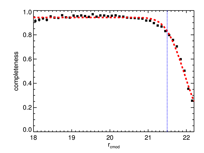
Figure 9 shows the completeness estimated for $r_{\mathrm{cmod}}$ detections for the median DR8 depth in the S82 fields. We model the completeness with a simple error function model:

$$c=(e/2)\left[1-\mathrm{erf}\left(\frac{m-m_{50}}{\sqrt{2w}}\right)\right],$$ (12)

where $e$ is the overall efficiency of detection at the bright end, $m_{50}$ is the magnitude at which the completeness is $50\%$, and $w$ is the (Gaussian) width of the rollover. The red dashed line in the plot shows the best-fit model, and the blue dotted line shows the median $10\sigma$ limit in the sampled region. The error bars are smaller than the data points at all but the brightest magnitudes. Although the model fit is not perfect, it clearly provides a reasonable description of the shape of the completeness function. The end result is that we now have measurements of $m_{50}$ and $w$ in bins of different survey depth $m_{\mathrm{lim}}$.

Figure 9.— Completeness estimated for $r_{\mathrm{cmod}}$ for Stripe 82 data for the median DR8 depth in the Stripe 82 fields. Red dashed line shows the fit of the functional form given by Eqn. 12. The blue dotted line shows the $10\sigma$ limiting magnitude. The error bars are smaller than the data points at all but the brightest magnitudes.

5.2. Completeness Results

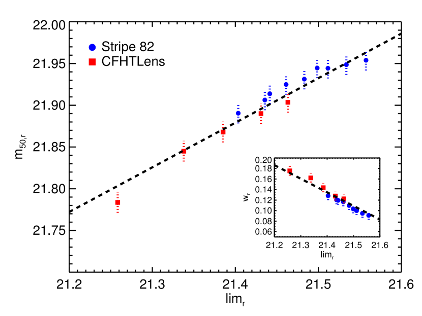
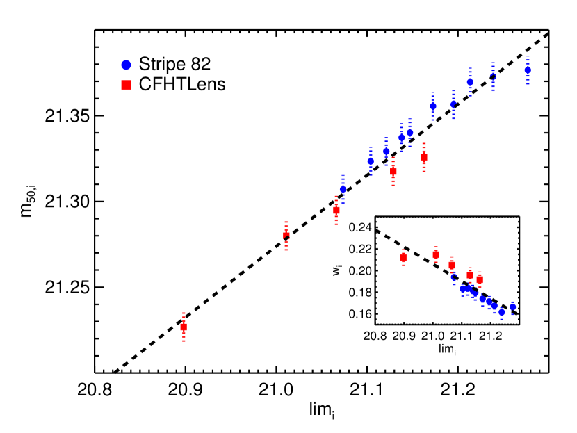
With these measurements in hand we determine how the galaxy completeness parameter $m_{50}$ depends on the survey depth parameter $m_{\mathrm{lim}}$. Figures 10 and 11 show the completeness as a function of the local limiting magnitude measured for $r_{\mathrm{cmod}}$ and $i_{\mathrm{cmod}}$ respectively. Blue circles show the results for S82 regions, and red squares for CFHTLens. The S82 regions tend to be deeper than average (as discussed in Section 3.2), and thus we sample a wide range of local depth with some overlap between the two data sets. The two data sets give consistent results, with a small systematic offset of $\sim 0.01$ magnitude. Solid error bars are those estimated from the bootstrap resampling, and the dashed error bars are an estimate of the systematic error required to yield $\chi^{2}/\mathrm{dof}=1$ for the linear fit.

Table 3 shows the final completeness parameter fits for $m_{50}$ and $w$. We note that both $m_{50}$ and $w$ are strong functions of the local limiting magnitude. Thus, in order to estimate the completeness at any point in the survey, we must first know the local depth.

Figure 10.— Main panel: Completeness parameter $m_{50}$, the magnitude at which $50\%$ of the galaxies are detected, as a function of local depth measured from $r_{\mathrm{cmod}}$. Blue circles are from S82, red squares from CFHTLens. Black dashed line is a linear fit. Inset:Width parameter $w$ as a function of local depth. Symbols are the same as the main panel.

Figure 11.— Same as Figure 10, with limiting magnitude measured from $i_{\mathrm{cmod}}$.

Table 3Completeness Fit Parameters

Magnitude	$a_{\mathrm{comp}}$	$b_{\mathrm{comp}}$	$a_{w}$	$b_{w}$
$r_{\mathrm{cmod}}$	$21.67\pm 0.02$	$0.53\pm 0.04$	$0.24\pm 0.01$	$-0.26\pm 0.03$
$i_{\mathrm{cmod}}$	$21.27\pm 0.01$	$0.41\pm 0.02$	$0.206\pm 0.003$	$-0.16\pm 0.02$

Note. — $m_{50}=a_{\mathrm{comp}}+b_{\mathrm{comp}}(\mathrm{lim}-21)$ ; $w=a_{w}+b_{w}(\mathrm{lim}-21)$

6. Impact on Correlation Functions

As an example of the use of these depth maps, we now investigate the impact on the estimation of correlation functions. The measurement of the correlation function $w(\theta)$ requires a set of random points that describes the window function of the observable (Landy & Szalay 1993). To first order, these random points can be sampled uniformly from the geometric mask of the survey. Although this works well at brighter magnitudes, when pushing the limits of a photometric survey this is certain to break down. In this section, we measure a simulated correlation function while comparing different methods of generating random points to show the utility of our method at faint magnitudes.

6.1. Generating a Simulated Survey

Our first task is to generate a simulated DR8-like survey with known systematics and known correlation function. We follow the same general plan as in Section 4.4, using a Monte Carlo technique to simulate data with uniform density (zero correlation). Consequently, any correlations observed in the data must necessarily be due to systematics being imprinted into the galaxy catalog.

There are two primary differences between this simulation and that from Section 4.4. The first is that we are building in the completeness estimation from Section 5. The second, is that we sample galaxies by color as well as magnitude to enable color selection in random point generation. Our procedure is as follows:

1. Generate simulated galaxies uniformly with zero correlation and approximately the same density as DR8 with $i_{\mathrm{cmod}}<21$.

2. Give each galaxy a true magnitude vector sampled from the (deeper) S82 catalog.

3. Estimate the completeness for each galaxy based on $i_{\mathrm{cmod}}$. Remove galaxies randomly according to the completeness estimate.

4. For each magnitude of each of the remaining galaxies, perturb the input magnitudes in accordance to the input survey depth map to yield a simulated survey as in Section 4.4.

As before, given this simulated survey we recompute the depth maps, fit the depth map, reconstruct a simulated high resolution depth map, and estimate the completeness from the simulated data. It is these re-estimated maps that are used in the following tests.

6.2. Generating Random Points

In order to measure the correlation function in real-space, we make use of the CORR2 code (Jarvis et al. 2004) for computing the Landy-Szalay statistic:

$$\Omega=\frac{DD-2DR+RR}{RR}.$$ (13)

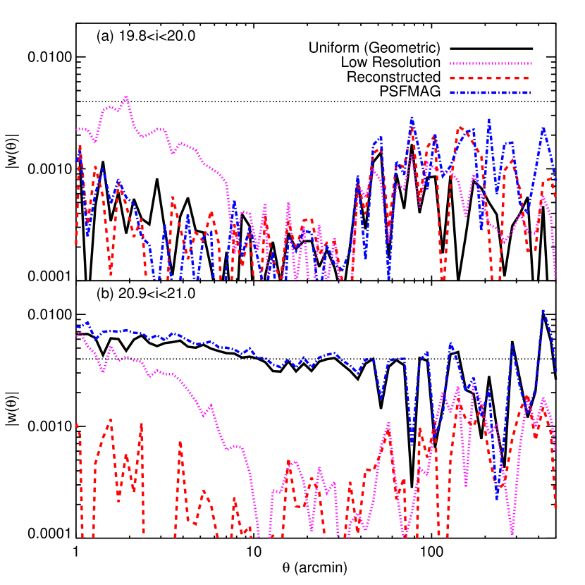
For our measurements, $D$ refers to the simulated galaxies, and $R$ refers to the random points used to sample the survey mask. We have chosen to compare the impact of four different methods of generating random points. These are:

1. “Uniform”: Only the geometric mask has been applied.

2. “Low Resolution”: The low resolution measured depth maps (NSIDE=256) are used. We also apply the completeness correction.

3. “Reconstructed”: The high resolution reconstructed depth maps (NSIDE=2048) are used. We also apply the completeness correction.

4. “PSFMAG”: The $5\sigma$ point-source psf magnitude depths from Section 4.5 are used, along with the derived constant offsets so the values match the $10\sigma$ galaxy depths on average. We also apply the completeness correction.

In all cases, the generation of random points follows the method for building the simulated survey galaxies in the first place. The primary difference is that we use the new reconstructed depth maps and re-estimated completeness. Therefore, the difference between the simulated survey galaxies and the random points is the noise in the estimation of the depth and completeness maps.

6.3. Results

In the interest of simplicity, we measure the correlation function for two magnitude cuts in $i$-band, and ignore the impact of the color selection. The first magnitude cut estimates the impact of depth variations on the correlation function for the faintest BOSS CMASS galaxies ($19.8<i_{\mathrm{cmod}}<20.0$; White et al. 2011; Ross et al. 2011; Ho et al. 2012). The second magnitude cut estimates the impact of depth variations on photometrically detected galaxies near the average $10\sigma$ survey limit, $20.9<i_{\mathrm{cmod}}<21.0$.

Figure 12 shows the absolute value of the two-point correlation function $|w(\theta)|$ estimated for various methods of generating random points. The dotted black line shows the typical error on $w(\theta)$ from Ho et al. (2012). Any additive bias on the correlation function below this level is sub-dominant. In the top panel, for the faintest CMASS galaxies with $19.8<i_{\mathrm{cmod}}<20.0$, we can see that uniform randoms (sold black line) are adequate to compute $w(\theta)$. Similarly, the other random point generation schemes, with the same geometric mask, all perform adequately. The only possible exception is the “Low Resolution” method (magenta dotted line) which may impart some structure at very small scales. In the bottom panel, for the galaxies near the $10\sigma$ photometric limit of the survey ($20.9<i_{\mathrm{cmod}}<21.0$), the choice of random points is much more significant. Using uniform random points (with the geometric mask) leads to significant residuals at all scales. The “PSFMAG” estimate of the depth (blue dot-dashed line) is better than uniform, but still has problems at all scales. The “Low Resolution” method works at large scales but not at small scales, while our full “Reconstructed” method (red dashed line) yields the best results, with only a small bias at the smallest scales. Therefore, we are confident that this method accurately captures depth and completeness variations down to faint magnitudes.

Figure 12.— Absolute value of the correlation function $|w(\theta)|$ for our simulated survey data using different sets of random points. Top Panel: Magnitude selection equivalent to the faintest BOSS CMASS galaxies, $19.8<i_{\mathrm{cmod}}<20.0$. The black dotted line shows the typical error on $w(\theta)$ from Ho et al. (2012). The solid black line shows the bias from using uniform randoms (with the geometric mask). The magenta dotted line shows the bias from the “Low Resolution” randoms. The red dashed line shows the bias from the full “Reconstructed” randoms, and the blue dot-dashed line shows the bias from the “PSFMAG” randoms. Bottom Panel: Same as above, for galaxies near the $10\sigma$ survey limit, $20.9<i_{\mathrm{cmod}}<21.0$. The impact on $w(\theta)$ for uniform randoms is large at all scales. Only the full reconstructed randoms show nearly unbiased results at all scales.

7. Results and Summary

In this paper, we have introduced a new way of empirically constructing depth maps from large photometric survey data. By combining low resolution depth maps with high resolution maps of survey systematics, we can use machine learning to reconstruct high resolution depth maps for typical galaxies measured using any arbitrary magnitude definition. Using SDSS DR8 as an example, our method can reconstruct the depth at an arbitrary point in the survey to within $\sim 2\%$, thus making it possible to accurately measure correlation functions for galaxies detected near the limiting magnitude of the survey. We emphasize that this method requires the knowledge of both a precise geometric mask, as well as accurate maps of the various systematics that affect galaxy photometry, especially seeing and sky brightness. Furthermore, the reported photometric errors in the data must be correct: any biases in the estimated photometric uncertainties of the detected galaxies will propagate into the survey depth maps.

In order to accurately build sets of random points suitable for correlation function measurements, a depth map is insufficient. We must also estimate the completeness function for galaxy detection. To estimate this function directly from the data, it is necessary to have data that is significantly deeper than the main survey. Fortunately, this is not only available for SDSS in the Stripe 82 coadds, but it is a common aspect of current and future wide-field surveys, including the Medium-Deep Survey fields in Pan-STARRs1 (Kaiser et al. 2002) and the supernova search fields in DES (The DES Collaboration 2005). We have shown that the completeness can be parametrized by a simple function for SDSS, and that the parameters of this function depend on the local survey depth. In this way, the depth map reconstruction is an essential prerequisite for estimating the local completeness of the survey.

As a sample of the utility of these depth maps, we demonstrate a new way of building random points for correlation function measurements that incorporates the full knowledge of the survey depth and local completeness. Uniform random points are sufficient when one is far from the photometric limit of the survey, as is the case for BOSS CMASS galaxies. These galaxies are relatively unaffected by variations in the local depth for two main reasons. First, the drift-scan technique ensures that SDSS is a relatively uniform survey, without large variations in depth. Second, we note that while SDSS uses the same telescope for both photometric and spectroscopic measurements, by necessity any spectroscopic target selection (such as CMASS) will necessarily be significantly brighter than the photometric limit for any reasonable balance of exposure time between the two surveys. Thus, it is not surprising that for the CMASS sample, designed for spectroscopic follow-up, uniform random points (with a proper geometric mask) are sufficient.

However, for ongoing and future photometric surveys, this will not be the case. In particular, both DES (The DES Collaboration 2005) and LSST (Ivezic et al. 2008) are purely photometric surveys where the best science will not be achieved by limiting measurements to galaxies more than a magnitude brighter than the survey limit. Furthermore, with tiled observations and chip gaps, depth variations will be much more significant than in SDSS, especially in the early phases before complete coverage is achieved. In addition, surveys such as the DECam Legacy Survey (DECaLS) will be used for target selection for the Dark Energy Spectrographic Instrument Survey (DESI) are not significantly deeper than the spectroscopic targeting. Therefore, we expect this method of building depth maps will be useful beyond the current application to SDSS.

Appendix A Reconstructed Depth Maps

The maps are available at http://risa.stanford.edu/redmapper. The list of maps are in Table 4. Each of them is in HEALPix FITS format, NSIDE=2048, ring ordered, equatorial coordinates.

Table 4List of HEALPix Maps

Band	Type	Name
$u$	model	sdss_dr8_nodered_nside2048_u_model_10sigma.fits.gz
$g$	model	sdss_dr8_nodered_nside2048_g_model_10sigma.fits.gz
$r$	model	sdss_dr8_nodered_nside2048_r_model_10sigma.fits.gz
$i$	model	sdss_dr8_nodered_nside2048_i_model_10sigma.fits.gz
$z$	model	sdss_dr8_nodered_nside2048_z_model_10sigma.fits.gz
$r$	cmodel	sdss_dr8_nodered_nside2048_r_cmodel_10sigma.fits.gz
$i$	cmodel	sdss_dr8_nodered_nside2048_i_cmodel_10sigma.fits.gz
	$E(B-V)$	sdss_dr8_ebv_sfd98_nside2048.fits.gz

Note. — All files are in HEALPix FITS format, NSIDE=2048, ring ordered, equatorial coordinates.

References

- Aihara et al. (2011) Aihara, H. et al. 2011, ApJS, 193, 29
- Annis et al. (2011) Annis, J. et al. 2011, ArXiv: 1111.6619
- Blake et al. (2010) Blake, C. et al. 2010, MNRAS, 406, 803
- Breiman (2001) Breiman, L. 2001, Machine Learning, 45, 5
- Dawson et al. (2013) Dawson, K. S. et al. 2013, AJ, 145, 10
- de Jong et al. (2015) de Jong, J. T. A. et al. 2015, ArXiv e-prints
- Erben et al. (2013) Erben, T. et al. 2013, MNRAS, 433, 2545
- Heymans et al. (2012) Heymans, C. et al. 2012, MNRAS, 427, 146
- Ho et al. (2012) Ho, S. et al. 2012, ApJ, 761, 14
- Ivezic et al. (2008) Ivezic, Z. et al. 2008, ArXiv e-prints
- Jarvis et al. (2004) Jarvis, M., Bernstein, G., & Jain, B. 2004, MNRAS, 352, 338
- Kaiser et al. (2002) Kaiser, N., et al. 2002, in Society of Photo-Optical Instrumentation Engineers (SPIE) Conference Series, Vol. 4836, Society of Photo-Optical Instrumentation Engineers (SPIE) Conference Series, ed. J. A. Tyson & S. Wolff, 154–164
- Landy & Szalay (1993) Landy, S. D., & Szalay, A. S. 1993, ApJ, 412, 64
- Liu et al. (2015) Liu, J., Petri, A., Haiman, Z., Hui, L., Kratochvil, J. M., & May, M. 2015, Phys. Rev. D, 91, 063507
- Nelder & Mead (1965) Nelder, J. A., & Mead, R. 1965, Computer Journal, 308
- Ross et al. (2011) Ross, A. J. et al. 2011, MNRAS, 417, 1350
- Rykoff et al. (2014) Rykoff, E. S., et al. 2014, ApJ, 785, 104
- Schlegel et al. (2009) Schlegel, D., White, M., & Eisenstein, D. 2009, in ArXiv Astrophysics e-prints, Vol. 2010, astro2010: The Astronomy and Astrophysics Decadal Survey, 314
- Schlegel et al. (1998) Schlegel, D. J., Finkbeiner, D. P., & Davis, M. 1998, ApJ, 500, 525
- Scranton et al. (2002) Scranton, R. et al. 2002, ApJ, 579, 48
- Suchyta et al. (2015) Suchyta, E. et al. 2015, ArXiv e-prints
- Swanson et al. (2008) Swanson, M. E. C., Tegmark, M., Hamilton, A. J. S., & Hill, J. C. 2008, MNRAS, 387, 1391
- The DES Collaboration (2005) The DES Collaboration. 2005, ArXiv: 0510346
- White et al. (2011) White, M. et al. 2011, ApJ, 728, 126
- York et al. (2000) York, D. G., Adelman, J., Anderson, J. E., Anderson, S. F., Annis, J., & the SDSS collaboration. 2000, AJ, 120, 1579