Complex Dynamics of $\displaystyle{z_{n+1}=\frac{\alpha+\beta z_{n}+\gamma z_{n-1}}{A+Bz_{n}+Cz_{n-1}}}$

Abstract

The dynamics of the second order rational difference equation $\displaystyle{z_{n+1}=\frac{\alpha+\beta z_{n}+\gamma z_{n-1}}{A+Bz_{n}+Cz_{n-1}}}$ with complex parameters and arbitrary complex initial conditions is investigated. In the complex set up, the local asymptotic stability and boundedness are studied vividly for this difference equation. Several interesting characteristics of the solutions of this equation, using computations, which does not arise when we consider the same equation with positive real parameters and initial conditions are shown. The chaotic solutions of the difference equation is absolutely new feature in the complex set up which is also shown in this article. Some of the interesting observations led us to pose some open interesting problems regarding chaotic and higher order periodic solutions and global asymptotic convergence of this equation.

Keywords: Rational difference equation, Local asymptotic stability, Chaotic trajectory and Periodicity.
Mathematics Subject Classification: 39A10, 39A11

1 Introduction and Preliminaries

A rational difference equation is a nonlinear difference equation of the form

$$z_{n+1}=\frac{\alpha+\sum_{i=0}^{k}\beta_{i}z_{n-i}}{A+\sum_{i=0}^{k}B_{i}z_{n-i}}$$

where the initial conditions $z_{0},z_{-1},\dots,z_{-k}$ are such that the denominator never vanishes for any $n$.
Consider the equation

$$z_{n+1}=\frac{\alpha+\beta z_{n}+\gamma z_{n-1}}{A+Bz_{n}+Cz_{n-1}},n=0,1,\ldots$$ (1)

where all the parameters and the initial conditions $z_{-1}$ and $z_{0}$ are arbitrary complex number.

This second order rational difference equation Eq.(1) is studied when the parameters are real numbers and initial conditions are non-negative real numbers in [2]. In this present article it is an attempt to understand the same in the complex plane.

Here, a very brief review of some well known results which will be useful in order to apprehend the behavior of solutions of the difference equation (1).

Let $f:\mathbb{D}^{2}\rightarrow\mathbb{D}$ where $\mathbb{D}\subseteq\mathbf{C}$ be a continuously differentiable function. Then for any pair of initial conditions $z_{0},z_{-1}\in\mathbb{D}$, the difference equation

$$z_{n+1}=f(z_{n},z_{n-1})\hskip 18.06749pt\hskip 18.06749pt$$ (2)

with initial conditions $z_{-1},z_{0}\in\mathbb{D}.$

Then for any initial value, the difference equation (1) will have a unique solution $\{z_{n}\}_{n}$.

A point $\overline{z}$ $\in$ $\mathbb{D}$ is called equilibrium point of Eq.(2) if

$$f(\overline{z},\overline{z})=\overline{z}.$$

The linearized equation of Eq.(2) about the equilibrium $\bar{z}$ is the linear difference equation

$${z_{n+1}=a_{0}z_{n}+a_{1}z_{n-1}\hskip 18.06749pt,\hskip 18.06749ptn=0,1,\ldots}$$ (3)

where for $i=0$ and $1$.

$$a_{i}=\frac{\partial f}{\partial u_{i}}(\overline{z},\overline{z}).$$

The characteristic equation of Eq.(2) is the equation

$$\lambda^{2}-a_{0}\lambda-a_{1}=0.$$ (4)

The following are the briefings of the linearized stability criterions which are useful in determining the local stability character of the equilibrium $\overline{z}$ of Eq.(2), [1].

Let $\overline{z}$ be an equilibrium of the difference equation $z_{n+1}=f(z_{n},z_{n-1})$.

• The equilibrium $\bar{z}$ of Eq. (2) is called locally stable if for every $\epsilon>0$, there exists a $\delta>0$ such that for every $z_{0}$ and $z_{-1}$ $\in$ $\mathbb{C}$ with $|z_{0}-\bar{z}|+|z_{-1}-\bar{z}|<\delta$ we have $|z_{n}-\bar{z}|<\epsilon$ for all $n>-1$.

• The equilibrium $\bar{z}$ of Eq. (2) is called locally stable if it is locally stable and if there exist a $\gamma>0$ such that for every $z_{0}$ and $z_{-1}$ $\in$ $\mathbb{C}$ with $|z_{0}-\bar{z}|+|z_{-1}-\bar{z}|<\gamma$ we have $\lim_{n\to\infty}z_{n}=\bar{z}$.

• The equilibrium $\bar{z}$ of Eq. (2) is called global attractor if for every $z_{0}$ and $z_{-1}$ $\in$ $\mathbb{C}$, we have $\lim_{n\to\infty}z_{n}=\bar{z}$.

• The equilibrium of equation Eq. (2) is called globally asymptotically stable/fit is stable and is a global attractor.

• The equilibrium $\bar{z}$ of Eq. (2) is called unstable if it is not stable.

• The equilibrium $\bar{z}$ of Eq. (2) is called source or repeller if there exists $r>0$ such that for every $z_{0}$ and $z_{-1}$ $\in$ $\mathbb{C}$ with $|z_{0}-\bar{z}|+|z_{-1}-\bar{z}|<r$ we have $|z_{n}-\bar{z}|\geq r$. Clearly a source is an unstable equilibrium.

Result 1.1: (Clark’s Theorem) The sufficient condition for the asymptotic stability of the difference equation (1) is

$$\left\lvert a_{0}\right\rvert+\left\lvert a_{1}\right\rvert<1$$

2 Difference Equation and Its Transformed Forms

The following difference equation is considered to be studied here.

$$z_{n+1}=\frac{\alpha+\beta z_{n}+\gamma z_{n-1}}{A+Bz_{n}+Cz_{n-1}},n=0,1,\ldots$$ (5)

where all the parameters are complex number and the initial conditions $z_{-1}$ and $z_{0}$ are arbitrary complex numbers.

We will consider three different cases of the Eq.(2) which are as follows:

2.1 The case $\beta=\gamma=0:z_{n+1}=\frac{\alpha}{A+Bz_{n}+Cz_{n-1}}$

By the change of variables, $z_{n}=\frac{\alpha}{A}w_{n}$, the difference equation $z_{n+1}=\frac{\alpha}{A+Bz_{n}+Cz_{n-1}}$ reduced to the difference equation

$$w_{n+1}=\frac{1}{1+pw_{n}+qw_{n-1}},n=0,1,\ldots$$ (6)

where $p=\frac{\alpha B}{A^{2}}$ and $q=\frac{\alpha C}{A^{2}}$.

2.2 The case $\alpha=\gamma=0:z_{n+1}=\frac{\beta z_{n}}{A+Bz_{n}+Cz_{n-1}}$

By the change of variables, $z_{n}=\frac{A}{C}w_{n}$, the difference equation $z_{n+1}=\frac{\beta z_{n}}{A+Bz_{n}+Cz_{n-1}}$ reduced to the difference equation

$$w_{n+1}=\frac{w_{n}}{1+pw_{n}+qw_{n-1}},n=0,1,\ldots$$ (7)

where $p=\frac{\beta}{A}$ and $q=\frac{B}{C}$.

2.3 The case $\alpha=\beta=0:z_{n+1}=\frac{\gamma z_{n-1}}{A+Bz_{n}+Cz_{n-1}}$

By the change of variables, $z_{n}=\frac{\gamma}{C}w_{n}$, the difference equation $z_{n+1}=\frac{\gamma z_{n-1}}{A+Bz_{n}+Cz_{n-1}}$ reduced to the difference equation

$$w_{n+1}=\frac{w_{n-1}}{p+qw_{n}+w_{n-1}},n=0,1,\ldots$$ (8)

where $p=\frac{A}{\gamma}$ and $q=\frac{B}{C}$.

Without any loss of generality, we shall now onward focus only on the three difference equations (6), (7) and (8).

3 Local Asymptotic Stability of the Equilibriums

In this section we establish the local stability character of the equilibria of Eq.(1) in three difference cases as stated in the section 2.

3.1 Local Asymptotic Stability of $w_{n+1}=\frac{1}{1+pw_{n}+qw_{n-1}}$

The equilibrium points of Eq.(6) are the solutions of the quadratic equation

$$\bar{w}=\frac{1}{1+p\bar{w}+q\bar{w}}$$

Eq.(6) has the two equilibria points $\bar{w}_{1,2}=\frac{-1-\sqrt{1+4p+4q}}{2(p+q)}$ and $\frac{-1+\sqrt{1+4p+4q}}{2(p+q)}$ respectively. The linearized equation of the rational difference equation(6) with respect to the equilibrium point $\bar{w}_{1}=\frac{-1-\sqrt{1+4p+4q}}{2(p+q)}$ is

$${z_{n+1}+\frac{4p}{\left(-1+\sqrt{1+4p+4q}\right)^{2}}w_{n}+\frac{4q}{\left(-1+\sqrt{1+4p+4q}\right)^{2}}w_{n-1}=0,n=0,1,\ldots}$$ (9)

with associated characteristic equation

$$\lambda^{2}+\frac{4p}{\left(-1+\sqrt{1+4p+4q}\right)^{2}}\lambda+\frac{4q}{\left(-1+\sqrt{1+4p+4q}\right)^{2}}=0.$$ (10)

The following result gives the local asymptotic stability of the equilibrium $\bar{w}_{1}$ of the Eq. (6).

Theorem 3.1.

The equilibriums $\bar{w}_{1}=\frac{-1-\sqrt{1+4p+4q}}{2(p+q)}$ of Eq.(6) is

locally asymptotically stable if

$$\left\lvert\frac{4p}{\left(-1+\sqrt{1+4p+4q}\right)^{2}}\right\rvert+\left\lvert{\frac{4q}{\left(-1+\sqrt{1+4p+4q}\right)^{2}}}\right\rvert<1$$

Proof.

The zeros of the characteristic equation (10) has two zeros which are $-\frac{2q}{p+\sqrt{p^{2}-4pq+2q\left(-1-2q+\sqrt{1+4p+4q}\right)}}$ and $\frac{2q}{-p+\sqrt{p^{2}-4pq+2q\left(-1-2q+\sqrt{1+4p+4q}\right)}}$. Therefore by Clark’s theorem, the equilibrium $\bar{w}_{1}=\frac{-1-\sqrt{1+4p+4q}}{2(p+q)}$ is locally asymptotically stable if the sum of the modulus of two coefficients is less than $1$. Therefore the condition of the polynomial (10) reduces to $\left\lvert\frac{4p}{\left(-1+\sqrt{1+4p+4q}\right)^{2}}\right\rvert+\left\lvert{\frac{4q}{\left(-1+\sqrt{1+4p+4q}\right)^{2}}}\right\rvert<1$.

∎

The linearized equation of the rational difference equation (6) with respect to the equilibrium point $\bar{w}_{2}=\frac{-1+\sqrt{1+4p+4q}}{2(p+q)}$ is

$${w_{n+1}+\frac{4p}{\left(1+\sqrt{1+4p+4q}\right)^{2}}w_{n}+\frac{4q}{\left(1+\sqrt{1+4p+4q}\right)^{2}}w_{n-1}=0,n=0,1,\ldots}$$ (11)

with associated characteristic equation

$$\lambda^{2}+\frac{4p}{\left(1+\sqrt{1+4p+4q}\right)^{2}}\lambda+-\frac{4q}{\left(1+\sqrt{1+4p+4q}\right)^{2}}=0.$$ (12)

Theorem 3.2.

The equilibriums $\bar{w}_{2}=\frac{-1+\sqrt{1+4p+4q}}{2(p+q)}$ of Eq.(6) is

locally asymptotically stable if

$$\left\lvert\frac{4p}{\left(1+\sqrt{1+4p+4q}\right)^{2}}\right\rvert+\left\lvert\frac{4q}{\left(1+\sqrt{1+4p+4q}\right)^{2}}\right\rvert<1$$

Proof.

Proof the theorem follows from Clark’s theorem of local asymptotic stability of the equilibriums. The condition for the local asymptotic stability reduces to $\left\lvert\frac{4p}{\left(1+\sqrt{1+4p+4q}\right)^{2}}\right\rvert+\left\lvert\frac{4q}{\left(1+\sqrt{1+4p+4q}\right)^{2}}\right\rvert<1$.

∎

Here is an example case for the local asymptotic stability of the equilibriums.

For $p=\frac{1}{2}$ and $q=\frac{i}{2}$ the equilibriums are $-1.6838+1.13355i$ and $0.683802-0.133552i$. For the equilibrium $1.6838+1.13355i$, the coefficients of the characteristic polynomial (10) are $0.775125+1.90868i$ and $-1.90868-0.775125i$ with same modulus $2.06006$. Therefore the condition as stated in the Theorem 3.1 does not hold. Therefore the equilibrium $1.6838+1.13355i$ is unstable.

For the equilibrium $0.683802-0.133552i$, the coefficients of the characteristic polynomial (12) are $-0.224875+0.091323i$ and $-0.091323-0.224875i$ with same modulus $0.242711$. Therefore the condition as stated in the Theorem 3.2 is hold good. Therefore the equilibrium $0.683802-0.133552i$ is locally asymptotically stable.

It is seen that in the case of real positive parameters and initials values, the positive equilibrium of the difference equation (6) is globally asymptotically stable [2]. But the result is not holding well in the complex set up.

3.2 Local Asymptotic Stability of $w_{n+1}=\frac{w_{n}}{1+pw_{n}+qw_{n-1}}$

The equilibrium points of Eq.(7) are the solutions of the quadratic equation

$$\bar{w}=\frac{\bar{w}}{1+p\bar{w}+q\bar{w}}$$

The Eq.(7) has only the zero equilibrium. The linearized equation of the rational difference equation(7) with respect to the zero equilibrium is

$${w_{n+1}=w_{n},n=0,1,\ldots}$$ (13)

with associated characteristic equation

$$\lambda^{2}-\lambda=0.$$ (14)

The following result gives the local asymptotic stability of the zero equilibrium of the Eq. (7).

Theorem 3.3.

The zero equilibriums of the Eq. (7) is non-hyperbolic.

Proof.

The zeros of the characteristic equation (14) has two zeros which are $0$ and $1$. Therefore by definition, the zero equilibrium is non-hyperbolic as the modulus of one zero is $1$. ∎

It is nice to note that in the case of real positive parameters and initials values, the zero equilibrium of the difference equation (7) is globally asymptotically stable for the parameter $p\geq 1$ [2]. But in the case of complex, the zero equilibrium is non-hyperbolic as we have seen the previous theorem.

3.3 Local Asymptotic Stability of $w_{n+1}=\frac{w_{n-1}}{p+qw_{n}+w_{n-1}}$

The equilibrium points of Eq.(8) are the solutions of the quadratic equation

$$\bar{w}=\frac{\bar{w}}{p+q\bar{w}+\bar{w}}$$

The Eq.(8) has two equilibriums which are $0$ and $\frac{1-p}{1+q}$. The linearized equation of the rational difference equation(8) with respect to the zero equilibrium is

$${w_{n+1}=\frac{1}{p}w_{n},n=0,1,\ldots}$$ (15)

with associated characteristic equation

$$\lambda^{2}-\frac{\lambda}{p}=0.$$ (16)

The following result gives the local asymptotic stability of the zero equilibrium of the Eq. (8).

Theorem 3.4.

The zero equilibriums of the Eq. (8) is locally asymptotically stable if $\left\lvert p\right\rvert\geq 1$ and repeller if $\left\lvert p\right\rvert<1$.

Proof.

The zeros of the characteristic equation (15) has two zeros which are $0$ and $\frac{1}{p}$. Therefore by definition, the zero equilibrium is locally asymptotically stable if $\left\lvert\frac{1}{p}\right\rvert<1$ and unstable (repeller) if $\left\lvert\frac{1}{p}\right\rvert\geq 1$. Hence the required is followed. ∎

The linearized equation of the rational difference equation(8) with respect to the equilibrium $\frac{1-p}{1+q}$ is

$${w_{n+1}=\frac{1+pq}{1+q}w_{n}+\frac{p-1}{1+q}w_{n-1}=0,n=0,1,\ldots}$$ (17)

with associated characteristic equation

$$\lambda^{2}-\frac{1+pq}{1+q}\lambda-\frac{p-1}{1+q}=0.$$ (18)

The following result gives the local asymptotic stability of the equilibrium $\frac{1-p}{1+q}$ of the Eq. (8).

Theorem 3.5.

The zero equilibriums of the Eq. (8) is locally asymptotically stable if

$$\left\lvert 1+pq\right\rvert+\left\lvert p-1\right\rvert<\left\lvert 1+q\right\rvert$$

Proof.

The equilibrium $\frac{1-p}{1+q}$ of the characteristic equation (18) would be locally asymptotically stable if the sum of the modulus of the coefficients of the characteristic equation (18) is less than 1. That is by Clark’s theorem, $\left\lvert\frac{1+pq}{1+q}\right\rvert+\left\lvert\frac{p-1}{1+q}\right\rvert<1$, that is

$$\left\lvert 1+pq\right\rvert+\left\lvert p-1\right\rvert<\left\lvert 1+q\right\rvert$$

∎

Here is an example case for the local asymptotic stability of the equilibriums.

For $p=1+\frac{i}{2}$ $(\left\lvert p\right\rvert=1.1180>1$) and $q=\frac{1}{10}+i$ ($\left\lvert q\right\rvert=1.005>1$) the equilibriums are $0$ and $-0.226244-0.248869i$. For the equilibrium $-0.226244-0.248869i$, the coefficients of the characteristic polynomial (18) are $0.533622+0.545503i$ and $-0.203409-0.0330197i$ with modulus $0.763103$ and $0.206072$ respectively. Therefore the condition as stated in the Theorem 3.5 hold good. Therefore the equilibrium $1.6838+1.13355i$ is locally asymptotically stable.

In the case of real positive parameters and intimal values of the difference equation (8), the positive equilibrium is locally asymptotically stable if $p<1$ and $q<1$ but in the complex set, it is encountered through the example above is that the equilibrium $\frac{1-p}{1+q}$ is locally asymptotically stable even though $\left\lvert p\right\rvert>1$ and $\left\lvert q\right\rvert>1$ [2].

4 Boundedness

In this section we would like to explore the boundedness of the solutions of the three difference equations (6), (7) and (8).

Now we would like to try to find open ball $B(0,\epsilon)\in\mathbf{C}$ such that if $w_{n}\in B(0,\epsilon)$ and $w_{n-1}\in B(0,\epsilon)$ then $w_{n+1}\in B(0,\epsilon)$ for all $n\geq 0$. In other words, if the initial values $w_{0}$ and $w_{-1}$ belong to $B(0,\epsilon)$ then the solution generated by the difference equations would essentially be within the open ball $B(0,\epsilon)$.

Theorem 4.1.

For the difference equation (6), for every $\epsilon>0$, if $w_{n}$ and $w_{n-1}$ $\in B(0,\epsilon)$ then $w_{n+1}\in B(0,\epsilon)$ provided

$$\left\lvert p\right\rvert\geq 1+\left\lvert q\right\rvert$$

Proof.

Let $\{w_{n}\}$ be a solution of the equation Eq.(6). Let $\epsilon>0$ be any arbitrary real number. Consider $w_{n},w_{n-1}\in B(0,\epsilon)$. We need to find out an $\epsilon$ such that $w_{n+1}\in B(0,\epsilon)$ for all $n$. It is follows from the Eq.(6) that for any $\epsilon>0$, using Triangle inequality for

$$\left\lvert w_{n+1}\right\rvert=\left\lvert\frac{1}{1+pw_{n}+qw_{n-1}}\right\rvert\leq\left\lvert\frac{1}{pw_{n}+qw_{n-1}}\right\rvert\leq\frac{1}{(\left\lvert p\right\rvert-\left\lvert q\right\rvert)\epsilon}$$

In order to ensure that $\left\lvert w_{n+1}\right\rvert<\epsilon^{\prime}$, (Assuming $\epsilon^{\prime}=\frac{1}{\epsilon}$) it is needed to be

$$\frac{1}{(\left\lvert p\right\rvert-\left\lvert q\right\rvert)}<1$$

That is $\left\lvert p\right\rvert\geq 1+\left\lvert q\right\rvert$. Therefore the required is followed.

∎

Theorem 4.2.

For the difference equation (7), for every $\epsilon>0$, if $w_{n}$ and $w_{n-1}$ $\in B(0,\epsilon)$ then $w_{n+1}\in B(0,\epsilon)$ provided

$$\left\lvert p\right\rvert\geq\left\lvert q\right\rvert+\frac{1}{\epsilon}$$

Proof.

Let $\{w_{n}\}$ be a solution of the equation Eq.(7). Let $\epsilon>0$ be any arbitrary real number. Consider $w_{n},w_{n-1}\in B(0,\epsilon)$. We need to find out an $\epsilon$ such that $w_{n+1}\in B(0,\epsilon)$ for all $n$. It is follows from the Eq.(7), that for any $\epsilon>0$, using Triangle inequality for

$$\left\lvert w_{n+1}\right\rvert=\left\lvert\frac{w_{n}}{1+pw_{n}+qw_{n-1}}\right\rvert\leq\frac{\epsilon}{(\left\lvert p\right\rvert-\left\lvert q\right\rvert)\epsilon}$$

Therefore, $\left\lvert w_{n+1}\right\rvert<\frac{1}{\left\lvert p\right\rvert-\left\lvert q\right\rvert}$. We need $\frac{1}{\left\lvert p\right\rvert-\left\lvert q\right\rvert}$ to be less than $\epsilon$. Therefore,

$$\left\lvert p\right\rvert\geq\left\lvert q\right\rvert+\frac{1}{\epsilon}$$

is followed.

∎

Theorem 4.3.

For the difference equation (8), for every $\epsilon>0$, if $w_{n}$ and $w_{n-1}$ $\in B(0,\epsilon)$ then $w_{n+1}\in B(0,\epsilon)$ and $\left\lvert p\right\rvert<1$ provided

$$\epsilon<\frac{\left\lvert p\right\rvert-1}{\left\lvert q\right\rvert+1}$$

Proof.

Let $\{w_{n}\}$ be a solution of the equation Eq.(8). Let $\epsilon>0$ be any arbitrary real number and $\left\lvert p\right\rvert>1$. Consider $w_{n},w_{n-1}\in B(0,\epsilon)$. We need to find out an $\epsilon$ such that $w_{n+1}\in B(0,\epsilon)$ for all $n$. It is follows from the Eq.(8), that for any $\epsilon>0$, using Triangle inequality for

$$\left\lvert w_{n+1}\right\rvert=\left\lvert\frac{w_{n-1}}{p+qw_{n}+w_{n-1}}\right\rvert\leq\frac{\epsilon}{\left\lvert p\right\rvert-\left\lvert q\right\rvert\epsilon-\epsilon}$$

Therefore,

$$\left\lvert w_{n+1}\right\rvert\leq\frac{\epsilon}{\left\lvert p\right\rvert-\left\lvert q\right\rvert\epsilon-\epsilon}$$

In order to ensure that $\left\lvert w_{n+1}\right\rvert<\epsilon$, it is needed to be

$$\frac{1}{\left\lvert p\right\rvert-\left\lvert q\right\rvert\epsilon-\epsilon}<1$$

That is

$$\epsilon<\frac{\left\lvert p\right\rvert-1}{\left\lvert q\right\rvert+1}$$

Therefore the required is followed.

∎

5 Periodic of Solutions

A solution $\{w_{n}\}_{n}$ of a difference equation is said to be globally periodic of period $t$ if $w_{n+t}=w_{n}$ for any given initial conditions. solution $\{w_{n}\}_{n}$ is said to be periodic with prime period $p$ if p is the smallest positive integer having this property.

We shall first look for the prime period two solutions of the three difference equations (6), (7) and (8) and their corresponding local stability analysis.

5.1 Prime Period Two Solutions of Eq. (6)

Let $\ldots,\phi,~{}\psi,~{}\phi,~{}\psi,\ldots$, $\phi\neq\psi$ be a prime period two solution of the difference equation $w_{n+1}=\frac{1}{1+pw_{n}+qw_{n-1}}$. Then $\phi=\frac{1}{1+p\psi+q\phi}$ and $\psi=\frac{1}{1+p\phi+q\psi}$. This two equations lead to the set of solutions (prime period two) except the equilibriums as $\left\{\phi\to\frac{0.5\left(p-q+\sqrt{p^{2}+p(-2-4q)q+q^{2}+4q^{3}}\right)}{q(-p+q)},\psi\to\frac{0.5p-0.5q-0.5\sqrt{p^{2}+p(-2-4q)q+q^{2}+4q^{3}}}{q(-p+q)}\right\}$ and $\left\{\phi\to\frac{q}{-0.5p+0.5q-0.5\sqrt{p^{2}+p(-2-4q)q+q^{2}+4q^{3}}},\psi\to\frac{-0.5-\frac{0.5\sqrt{p^{2}+p(-2-4q)q+q^{2}+4q^{3}}}{p-q}}{q}\right\}$.

Let $\ldots,\phi,~{}\psi,~{}\phi,~{}\psi,\ldots$, $\phi\neq\psi$ be a prime period two solution of the equation (6). We set

$$u_{n}=w_{n-1}$$

$$v_{n}=w_{n}$$

Then the equivalent form of the difference equation (6) is

$$u_{n+1}=v_{n}$$

$$v_{n+1}=\frac{1}{1+pv_{n}+qu_{n}}$$

Let T be the map on $\mathbb{C}\times\mathbb{C}$ to itself defined by

$$T\left(\begin{array}[]{c}u\\ v\\ \end{array}\right)=\left(\begin{array}[]{c}v\\ \frac{1}{1+pv+qu}\\ \end{array}\right)$$

Then $\left(\begin{array}[]{c}\phi\\ \psi\\ \end{array}\right)$ is a fixed point of $T^{2}$, the second iterate of $T$.

$$T^{2}\left(\begin{array}[]{c}u\\ v\\ \end{array}\right)=\left(\begin{array}[]{c}\frac{1}{1+pv+qu}\\ \\ \frac{1}{1+p\frac{1}{1+pv+qu}+qv}\\ \end{array}\right)$$

$$T^{2}\left(\begin{array}[]{c}u\\ v\\ \end{array}\right)==\left(\begin{array}[]{c}g(u,v)\\ h(u,v)\\ \end{array}\right)$$

where $g(u,v)=\frac{1}{1+pv+qu}$ and $h(u,v)=\frac{1}{1+\frac{p}{1+\text{pv}+\text{qu}}+\text{qv}}$. Clearly the two cycle is locally asymptotically stable when the eigenvalues of the Jacobian matrix $J_{T^{2}}$, evaluated at $\left(\begin{array}[]{c}\phi\\ \psi\\ \end{array}\right)$ lie inside the unit disk.

We have,

$$J_{T^{2}}\left(\begin{array}[]{c}\phi\\ \psi\\ \end{array}\right)=\left(\begin{array}[]{cc}\frac{\delta g}{\delta u}(\phi,\psi)&\frac{\delta g}{\delta v}(\phi,\psi)\\ \\ \frac{\delta h}{\delta u}(\phi,\psi)&\frac{\delta h}{\delta v}(\phi,\psi)\\ \end{array}\right)$$

where $\frac{\delta g}{\delta u}(\phi,\psi)=-\frac{q}{(1+q\phi+p\psi)^{2}}$ and $\frac{\delta g}{\delta v}(\phi,\psi)=-\frac{p}{(1+q\phi+p\psi)^{2}}$

$\frac{\delta h}{\delta u}(\phi,\psi)=\frac{pq}{\left((1+q\phi)(1+q\psi)+p\left(1+\psi+q\psi^{2}\right)\right)^{2}}$ and $\frac{\delta h}{\delta v}(\phi,\psi)=\frac{-q+\frac{p^{2}}{(1+q\phi+p\psi)^{2}}}{\left(1+q\psi+\frac{p}{1+q\phi+p\psi}\right)^{2}}$

Now, set

$$\chi=\frac{\delta g}{\delta u}(\phi,\psi)+\frac{\delta h}{\delta v}(\phi,\psi)=-\frac{q}{(1+q\phi+p\psi)^{2}}+\frac{-q+\frac{p^{2}}{(1+q\phi+p\psi)^{2}}}{\left(1+q\psi+\frac{p}{1+q\phi+p\psi}\right)^{2}}$$

$$\lambda=\frac{\delta g}{\delta u}(\phi,\psi)\frac{\delta h}{\delta v}(\phi,\psi)-\frac{\delta g}{\delta v}(\phi,\psi)\frac{\delta h}{\delta u}(\phi,\psi)=\frac{q^{2}}{\left((1+q\phi)(1+q\psi)+p\left(1+\psi+q\psi^{2}\right)\right)^{2}}$$

In particular for the prime period $2$ solution,

$\left\{\phi\to\frac{0.5\left(p-q+\sqrt{p^{2}+p(-2-4q)q+q^{2}+4q^{3}}\right)}{q(-p+q)},\psi\to\frac{0.5p-0.5q-0.5\sqrt{p^{2}+p(-2-4q)q+q^{2}+4q^{3}}}{q(-p+q)}\right\}$, we shall see the local asymptotic stability for some example cases of parameters $p$ and $q$. The general form of $\chi$ and $\lambda$ would be very complected. Consider the prime period two solution of the difference equation (6), $\phi\to-0.0843748+0.0622145i,\psi\to-0.0822456-0.0594374i$ corresponding two the parameters $p\to 100+i$ and $q\to 6+0.1i$.

In this case, $\left\lvert\chi\right\rvert=0.0735211$ and $\left\lvert\lambda\right\rvert=0.004075$. Therefore, by the Linear Stability theorem ($|\chi|<1+|\lambda|<2$) the prime period $2$ solution $\phi\to-0.0843748+0.0622145i,\psi\to-0.0822456-0.0594374i$ is locally asymptotically stable.

5.2 Prime Period Two Solutions of Eq. (7)

Let $\ldots,\phi,~{}\psi,~{}\phi,~{}\psi,\ldots$, $\phi\neq\psi$ be a prime period two solution of the difference equation $w_{n+1}=\frac{w_{n}}{1+pw_{n}+qw_{n-1}}$. Then $\phi=\frac{\psi}{1+p\psi+q\phi}$ and $\psi=\frac{\phi}{1+p\phi+q\psi}$. This two equations lead to the set of solutions (prime period two) except the equilibriums as $\left\{\phi\to\frac{1}{0.5p-0.5q-0.5\sqrt{p^{2}-q^{2}}},\psi\to-\frac{1}{q}+\frac{\sqrt{p^{2}-q^{2}}}{pq-q^{2}}\right\},\left\{\phi\to\frac{1}{0.5p-0.5q+0.5\sqrt{p^{2}-q^{2}}},\psi\to-\frac{1}{q}-\frac{\sqrt{p^{2}-q^{2}}}{pq-q^{2}}\right\}$.

Let $\ldots,\phi,~{}\psi,~{}\phi,~{}\psi,\ldots$, $\phi\neq\psi$ be a prime period two solution of the equation (7). We set

$$u_{n}=w_{n-1}$$

$$v_{n}=w_{n}$$

Then the equivalent form of the difference equation (7) is

$$u_{n+1}=v_{n}$$

$$v_{n+1}=\frac{v_{n}}{1+pv_{n}+qu_{n}}$$

Let T be the map on $\mathbb{C}\times\mathbb{C}$ to itself defined by

$$T\left(\begin{array}[]{c}u\\ v\\ \end{array}\right)=\left(\begin{array}[]{c}v\\ \frac{v}{1+pv+qu}\\ \end{array}\right)$$

Then $\left(\begin{array}[]{c}\phi\\ \psi\\ \end{array}\right)$ is a fixed point of $T^{2}$, the second iterate of $T$.

$$T^{2}\left(\begin{array}[]{c}u\\ v\\ \end{array}\right)=\left(\begin{array}[]{c}\frac{v}{1+pv+qu}\\ \\ \frac{\frac{v}{1+pv+qu}}{1+p\frac{v}{1+pv+qu}+qv}\\ \end{array}\right)$$

$$T^{2}\left(\begin{array}[]{c}u\\ v\\ \end{array}\right)==\left(\begin{array}[]{c}g(u,v)\\ h(u,v)\\ \end{array}\right)$$

where $g(u,v)=\frac{v}{1+pv+qu}$ and $h(u,v)=\frac{\frac{v}{1+pv+qu}}{1+p\frac{v}{1+pv+qu}+qv}$. Clearly the two cycle is locally asymptotically stable when the eigenvalues of the Jacobian matrix $J_{T^{2}}$, evaluated at $\left(\begin{array}[]{c}\phi\\ \psi\\ \end{array}\right)$ lie inside the unit disk.

We have,

$$J_{T^{2}}\left(\begin{array}[]{c}\phi\\ \psi\\ \end{array}\right)=\left(\begin{array}[]{cc}\frac{\delta g}{\delta u}(\phi,\psi)&\frac{\delta g}{\delta v}(\phi,\psi)\\ \\ \frac{\delta h}{\delta u}(\phi,\psi)&\frac{\delta h}{\delta v}(\phi,\psi)\\ \end{array}\right)$$

where $\frac{\delta g}{\delta u}(\phi,\psi)=-\frac{q\psi}{(1+q\phi+p\psi)^{2}}$ and $\frac{\delta g}{\delta v}(\phi,\psi)=\frac{1+q\phi}{(1+q\phi+p\psi)^{2}}$

$\frac{\delta h}{\delta u}(\phi,\psi)=-\frac{q\psi(1+q\psi)}{\left(1+\psi+p\psi+q\left(\phi+\psi+q\phi\psi+p\psi^{2}\right)\right)^{2}}$ and $\frac{\delta h}{\delta v}(\phi,\psi)=\frac{1+q\left(\phi-p\psi^{2}\right)}{\left(1+\psi+p\psi+q\left(\phi+\psi+q\phi\psi+p\psi^{2}\right)\right)^{2}}$

Now, set

$$\chi=\frac{\delta g}{\delta u}(\phi,\psi)+\frac{\delta h}{\delta v}(\phi,\psi)=-\frac{q\psi}{(1+q\phi+p\psi)^{2}}+\frac{1+q\left(\phi-p\psi^{2}\right)}{\left(1+\psi+p\psi+q\left(\phi+\psi+q\phi\psi+p\psi^{2}\right)\right)^{2}}$$

$$\lambda=\frac{q^{2}\psi^{2}}{(1+q\phi+p\psi)\left(1+\psi+p\psi+q\left(\phi+\psi+q\phi\psi+p\psi^{2}\right)\right)^{2}}$$

In particular for the prime period $2$ solution,

$\left\{\phi\to\frac{1}{0.5p-0.5q-0.5\sqrt{p^{2}-q^{2}}},\psi\to-\frac{1}{q}+\frac{\sqrt{p^{2}-q^{2}}}{pq-q^{2}}\right\}$, we shall see the local asymptotic stability for some example cases of parameters $p$ and $q$. The general form of $\chi$ and $\lambda$ would very complected. Consider the prime period two solution of the difference equation (7), $\phi\to 0.365026+0.263198i,\psi\to-0.412345+0.131124i$ corresponding two the parameters $p\to\frac{1}{5}+3i$ and $q\to\frac{3}{5}+5i$.

In this case, $\left\lvert\chi\right\rvert=0.0287948$ and $\left\lvert\lambda\right\rvert=0.0000431717$. Therefore, by the Linear Stability theorem ($|\chi|<1+|\lambda|<2$) the prime period $2$ solution $\phi\to 0.365026+0.263198i,\psi\to-0.412345+0.131124i$ is locally asymptotically stable.

5.3 Prime Period Two Solutions of Eq. (8)

Let $\ldots,\phi,~{}\psi,~{}\phi,~{}\psi,\ldots$, $\phi\neq\psi$ be a prime period two solution of the difference equation $w_{n+1}=\frac{w_{n-1}}{p+qw_{n}+w_{n-1}}$. Then $\phi=\frac{\phi}{1+p\psi+q\phi}$ and $\psi=\frac{\psi}{1+p\phi+q\psi}$. This two equations lead to the set of solutions (prime period two) except the equilibriums as $\left\{\phi\to 0,\psi\to 1-p\right\}$.

Let $\ldots,\phi,~{}\psi,~{}\phi,~{}\psi,\ldots$, $\phi\neq\psi$ be a prime period two solution of the equation (8). We set

$$u_{n}=w_{n-1}$$

$$v_{n}=w_{n}$$

Then the equivalent form of the difference equation (8) is

$$u_{n+1}=v_{n}$$

$$v_{n+1}=\frac{u_{n}}{p+qv_{n}+u_{n}}$$

Let T be the map on $\mathbb{C}\times\mathbb{C}$ to itself defined by

$$T\left(\begin{array}[]{c}u\\ v\\ \end{array}\right)=\left(\begin{array}[]{c}v\\ \frac{u}{p+qv+u}\\ \end{array}\right)$$

Then $\left(\begin{array}[]{c}\phi\\ \psi\\ \end{array}\right)$ is a fixed point of $T^{2}$, the second iterate of $T$.

$$T^{2}\left(\begin{array}[]{c}u\\ v\\ \end{array}\right)=\left(\begin{array}[]{c}\frac{u}{p+qv+u}\\ \\ \frac{\frac{u}{p+qv+u}}{p+q\frac{u}{p+qv+u}+v}\\ \end{array}\right)$$

$$T^{2}\left(\begin{array}[]{c}u\\ v\\ \end{array}\right)==\left(\begin{array}[]{c}g(u,v)\\ h(u,v)\\ \end{array}\right)$$

where $g(u,v)=\frac{u}{p+qv+u}$ and $h(u,v)=\frac{\frac{u}{p+qv+u}}{p+q\frac{u}{p+qv+u}+v}$. Clearly the two cycle is locally asymptotically stable when the eigenvalues of the Jacobian matrix $J_{T^{2}}$, evaluated at $\left(\begin{array}[]{c}\phi\\ \psi\\ \end{array}\right)$ lie inside the unit disk.

We have,

$$J_{T^{2}}\left(\begin{array}[]{c}\phi\\ \psi\\ \end{array}\right)=\left(\begin{array}[]{cc}\frac{\delta g}{\delta u}(\phi,\psi)&\frac{\delta g}{\delta v}(\phi,\psi)\\ \\ \frac{\delta h}{\delta u}(\phi,\psi)&\frac{\delta h}{\delta v}(\phi,\psi)\\ \end{array}\right)$$

where $\frac{\delta g}{\delta u}(\phi,\psi)=\frac{p+q\psi}{(p+\phi+q\psi)^{2}}$ and $\frac{\delta g}{\delta v}(\phi,\psi)=-\frac{q\phi}{(p+\phi+q\psi)^{2}}$

$\frac{\delta h}{\delta u}(\phi,\psi)=\frac{(1+\psi)(p+q\psi)}{\left(p+\phi+q\phi+(p+q+\phi)\psi+q\psi^{2}\right)^{2}}$ and $\frac{\delta h}{\delta v}(\phi,\psi)=-\frac{\phi(p+q+\phi+2q\psi)}{\left(p+\phi+q\phi+(p+q+\phi)\psi+q\psi^{2}\right)^{2}}$

Now, set

$$\chi=\frac{\delta g}{\delta u}(\phi,\psi)+\frac{\delta h}{\delta v}(\phi,\psi)=\frac{p+q\psi}{(p+\phi+q\psi)^{2}}-\frac{\phi(p+q+\phi+2q\psi)}{\left(p+\phi+q\phi+(p+q+\phi)\psi+q\psi^{2}\right)^{2}}$$

$$\lambda=-\frac{\phi(p+q\psi)}{(p+\phi+q\psi)\left(p+\phi+q\phi+(p+q+\phi)\psi+q\psi^{2}\right)^{2}}$$

For the prime period $2$ solution, $\phi\to 0,\psi\to 1-p$, $\chi=\frac{1}{p+(1-p)q}$ and $\left\lvert\lambda\right\rvert=0$. Therefore, by the Linear Stability theorem ($|\chi|<1+|\lambda|<2$) the prime period $2$ solution is locally asymptotically stable if and only if $\left\lvert\frac{1}{p+(1-p)q}\right\rvert<1$. It turns out that $\left\lvert q\right\rvert>\frac{1-\left\lvert p\right\rvert}{\left\lvert 1-p\right\rvert}$. In other words, the condition reduces to $\left\lvert p\right\rvert<1$ and $\left\lvert q\right\rvert>1$ which is same condition as it was for the real set up.

6 Chaotic Solutions

This is something which is absolutely new feature of the dynamics of the difference equation (1) which did not arise in the real set up of the same difference equation. Computationally we have encountered some chaotic solution of the difference equation (8) for some parameter values which are given in the following Table. 1.
The method of Lyapunov characteristic exponents serves as a useful tool to quantify chaos. Specifically Lyapunav exponents measure the rates of convergence or divergence of nearby trajectories. Negative Lyapunov exponents indicate convergence, while positive Lyapunov exponents demonstrate divergence and chaos. The magnitude of the Lyapunov exponent is an indicator of the time scale on which chaotic behavior can be predicted or transients decay for the positive and negative exponent cases respectively. In this present study, the largest Lyapunov exponent is calculated for a given solution of finite length numerically [10].
From computational evidence, it is arguable that for complex parameters $p$ and $q$ which are stated in the following table the solutions are chaotic for every initial values.

Parameters $p$, $q$	Interval of Lyapunav exponent
$p=(0.2037,0.5444)$, $q=(0.8749,0.1210)$	$(0.3215,1.6235)$
$p=(0.4933,0.7018)$, $q=(0.8878,0.0551)$	$(1.062,2.021)$
$p=(0.7840,0.4867)$, $q=(0.4648,0.1313)$	$(0.6256,1.314)$
$p=(0.2308,0.6580)$, $q=(0.5629,0.2818)$	$(1.373,2.325)$

Table 1: Chaotic solutions of the equation (8) for different choice of parameters and initial values.

The chaotic trajectory plots including corresponding complex plots are given the following Fig. 1.

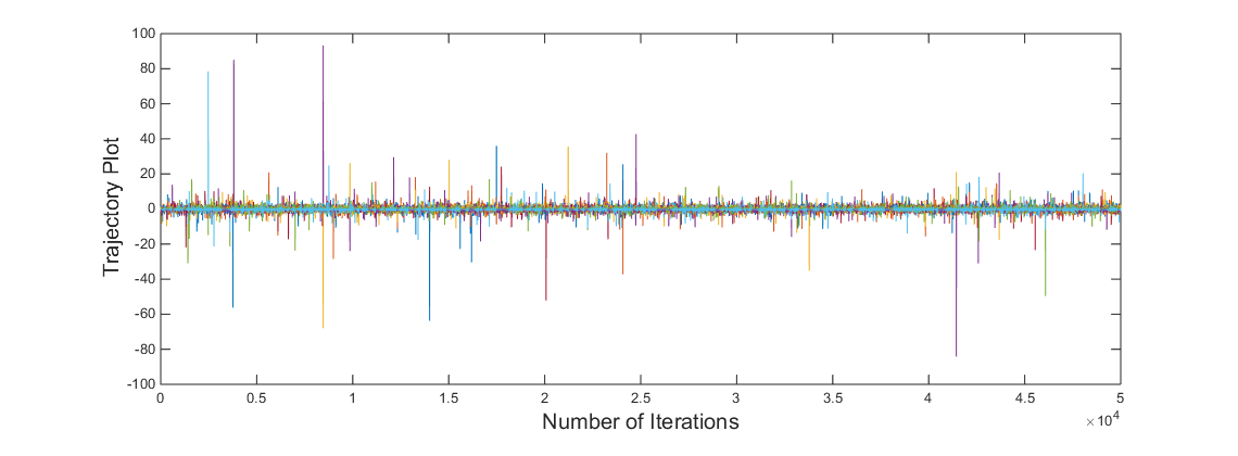
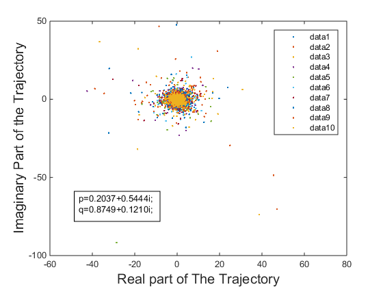
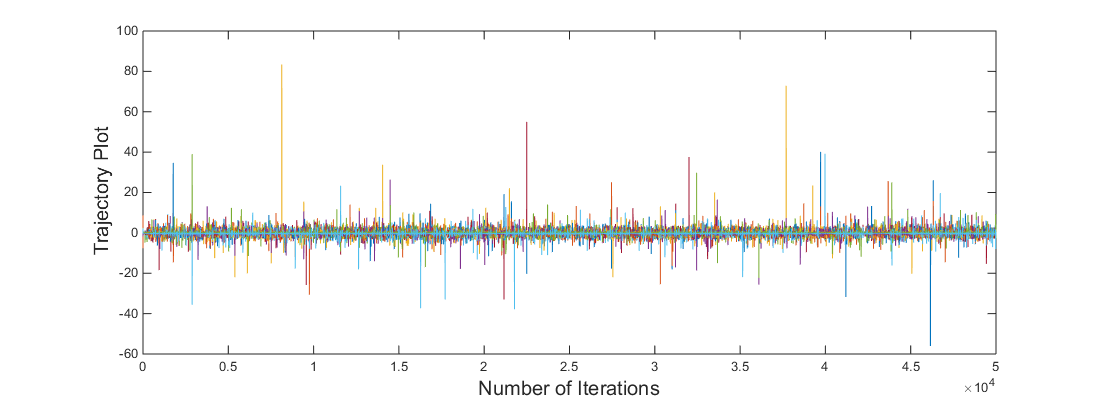
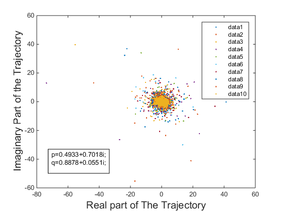
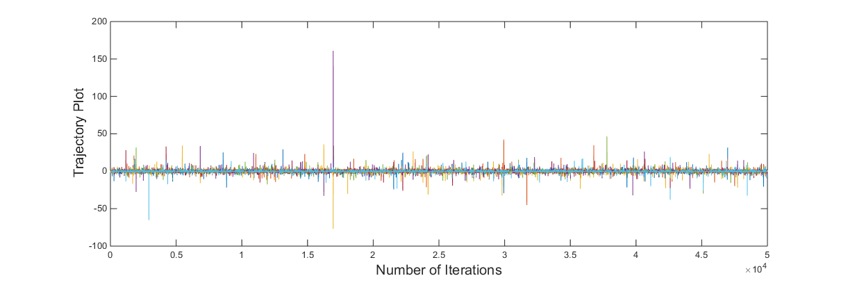
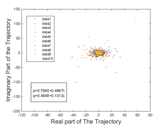
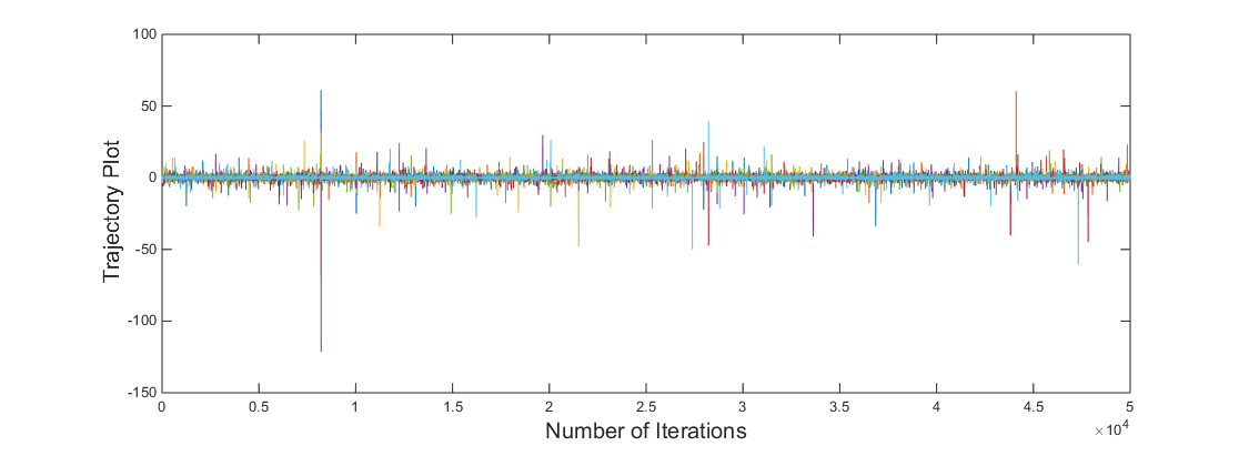
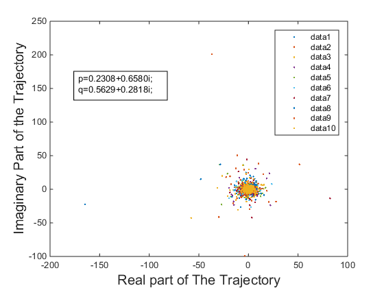
Figure 1: Chaotic Trajectories of the equation (8) of four different cases as stated in Table 1.

In the Fig. 1, for each of the four cases ten different initial values are taken and plotted in the left and in the right corresponding complex plots are given. From the Fig. 1, it is evident that for the four different cases the basin of the chaotic attractor is neighbourhood of the centre $(0,0)$ of complex plane.

7 Some Interesting Nontrivial Problems

Open Problem 7.1.

Does the difference equation have higher order periodic cycle? If so, what is the highest periodic cycle?

Open Problem 7.2.

Find out the set of all parameters $p$ and $q$ for which the difference equation (8) has chaotic solutions.

Open Problem 7.3.

Find out the subset of the $\mathbb{D}$ of all possible initial values $z_{0}$ and $z_{1}$ for which the solutions of the difference equation are chaotic for any complex parameters $p$ and $q$. Does the neighbourhood of $(0,0)$ is global chaotic attractor? If not, are there any other chaotic attractors?

8 Future Endeavours

In continuation of the present work the study of the difference equation ${z_{n+1}=\frac{\alpha_{n}+\beta_{n}z_{n}+\gamma_{n}z_{n-1}}{A_{n}+B_{n}z_{n}+C_{n}z_{n-1}}}$ where $\alpha_{n}$, $\beta_{n}$, $\gamma_{n}$, $A_{n}$, $B_{n}$ and $C_{n}$ are all convergent sequence of complex numbers and converges to $\alpha$, $\beta$, $\gamma$, $A$, $B$ and $C$ respectively is indeed would be very interesting and that we would like to pursue further. Also the most generalization of the present rational difference equation is

$${z_{n+1}=\frac{\alpha+\beta z_{n-l}+\gamma z_{n-k}}{A+Bz_{n-l}+Cz_{n-k}}}$$

where $l$ and $k$ are delay terms and it demands similar analysis which we plan to pursue in near future.

References

• [1] Saber N Elaydi, Henrique Oliveira, JosΓ© Manuel Ferreira and JoΓ£o F Alves, Discrete Dyanmics and Difference Equations, Proceedings of the Twelfth International Conference on Difference Equations and Applications, World Scientific Press, 2007.
• [2] S. Atawna, R. Abu-Saris, E. S. Ismail, and I. Hashim, Stability of Nonhyperbolic Equilibrium Solution of Second Order Nonlinear Rational Difference Equation, Journal of Difference Equations Volume 2015 (2015), Article ID 486985.
• [3] Ch. G. Philos, I. K. Purnaras, and Y. G. Sficas, Global attractivity in a nonlinear difference equation, Appl. Math. Comput. 62(1994), 249-258.
• [4] E. Camouzis and G. Ladas, Dynamics of Third Order Rational Difference Equations; With Open Problems and Conjectures, Chapman & Hall/CRC Press, 2008.
• [5] N. K. Govil and Q, I. Rahman, On the EnestrΓΆm-Kakeya theorem, Tohoku Mathematical Journal, 20(1968), 126-136.
• [6] E. Camouzis, E. Chatterjee, G. Ladas and E. P. Quinn, On Third Order Rational Difference Equations – Open Problems and Conjectures, Journal of Difference Equations and Applications, 10(2004), 1119 – 1127.
• [7] G. T. Cargo and O. Shisha, Zeros of polynomials and fractional order differences of their coefficients, Journ. Math. Anal. Appl., 7 (1963), 176-182.
• [8] A. Joyal, G. Labelle and Q.I.Rahaman, On the location of zeros of polynomials, Canad. Math. Bull., 10 (1967), 53-63.
• [9] P. V. Krishnaiah, On Kakeya’s theorem, Journ. London Math. Soc., 30 (1955), 314-319.
• [10] A. Wolf, J. B. Swift, H. L. Swinney and J. A. Vastano, Determining Lyapunov exponents from a time series Physica D, 126(1985), 285-317.
• [11] E.A. Grove, Y. Kostrov and S.W. Schultz, On Riccati Difference Equations With Complex Coefficients, Proceedings of the 14th International Conference on Difference Equations and Applications, Istanbul, Turkey, March 2009.
• [12] Sk. S. Hassan, E. Chatterjee, Dynamics of the equation $\displaystyle{z_{n+1}=\frac{\alpha+\beta z_{n}}{A+z_{n-1}}}$ in the Complex Plane, Communicated to Computational Mathematics and Mathematical Physics, Springer, 2014
• [13] M.R.S. Kulenovi$\acute{c}$ and G. Ladas, Dynamics of Second Order Rational Difference Equations; With Open Problems and Conjectures, Chapman & Hall/CRC Press, 2001.
• [14] V.L. Kocic and G. Ladas, Global Behaviour of Nonlinear Difference Equations of Higher Order with Applications, Kluwer Academic Publishers, Dordrecht, Holland, 1993.
• [15] Sk. S. Hassan, P. Basu, Complex Dynamics of the Difference Equation $z_{n+1}=\frac{\alpha}{z_{n}}+\frac{\beta}{z_{n-1}}$, arXiv:1502.06469 [math.DS].