Analytical prediction for the optical matrix

Abstract

Contrary to praxis, we provide an analytical expression, for a physical locally periodic structure, of the average $\langle S\rangle$ of the scattering matrix, called optical $S$ matrix in the nuclear physics jargon, and fundamentally present in all scattering processes. This is done with the help of a strictly analogous nonlinear dynamical mapping where iteration time is the number $N$ of scatterers. The ergodic property of chaotic attractors implies the existence and analyticity of $\langle S\rangle$. We find that the optical $S$ matrix depends only on the transport properties of a single cell, and that the Poisson kernel is the distribution of the scattering matrix $S_{N}$ in the large size limit $N\rightarrow\infty$. The theoretical distribution shows perfect agreement with numerical results for a chain of delta potentials. A consequence of our findings is the a priori knowledge of $\langle S\rangle$ without resort to experimental data.

Scattering is an outstanding phenomenon of nature concerning waves and particles NewtonBook . It is important in almost all branches of physics since many physical observables, at microscopic and macroscopic scales, are described in terms of scattering properties Krane ; MelloBook ; Landauer ; Buttiker1 ; Buttiker2 ; Brouwer1 ; Brouwer2 ; Doron ; Schanze1 ; Mendez ; Hemmady ; FloresO . In experiments, the scattering amplitudes vary with respect to a tuning parameter which could be the energy of incidence in nuclear, many body, and atomic physics Orrigo ; Watson ; Silvestri , the Fermi energy or an applied magnetic field in condensed matter physics Keller ; Marcus , and the frequency in optics Tribelsky , microwaves Schanze1 ; Mendez ; Kuhl ; Schanze2 ; Sirko , and elastic systems Marcel ; FloresO .

Irrespective of the different mechanisms that occur in complex scattering processes, the wave amplitudes contain a direct (rapid) component and an equilibrated (delayed) multiple-scattering component. The rapid response is revealed by the average of the measured scattering amplitudes over an interval of the corresponding tuning parameter, the so called optical amplitudes LMS . The delayed response is obtained by subtracting the direct response to the set of measured scattering amplitudes. The scattering matrix samples amplitude values according to a range or space fixed by the current value of the tuning parameter. The way in which the values of the scattering matrix are distributed along this space is determined once the optical $S$ matrix is specified, any other information being irrelevant MelloLesHouches .

The scattering amplitudes fluctuate around their average values or from sample-to-sample, so that, in a statistical-mechanical fashion, the construction of an ensemble of scattering systems together with an ergodic hypothesis is used to obtain a quantitative description of the scattering process. The direct response component is corroborated via comparison with the ensemble average of the scattering amplitudes at a fixed tuning parameter LMS ; MPS . In all cases $\langle S\rangle$ is determined from the experimental or numerical data. The question we address here is whether there exists the possibility to predict the matrix $\langle S\rangle$ via a procedure that does not require obtaining the average from the experiment, actual or numeric, but follows instead from a scattering formalism.

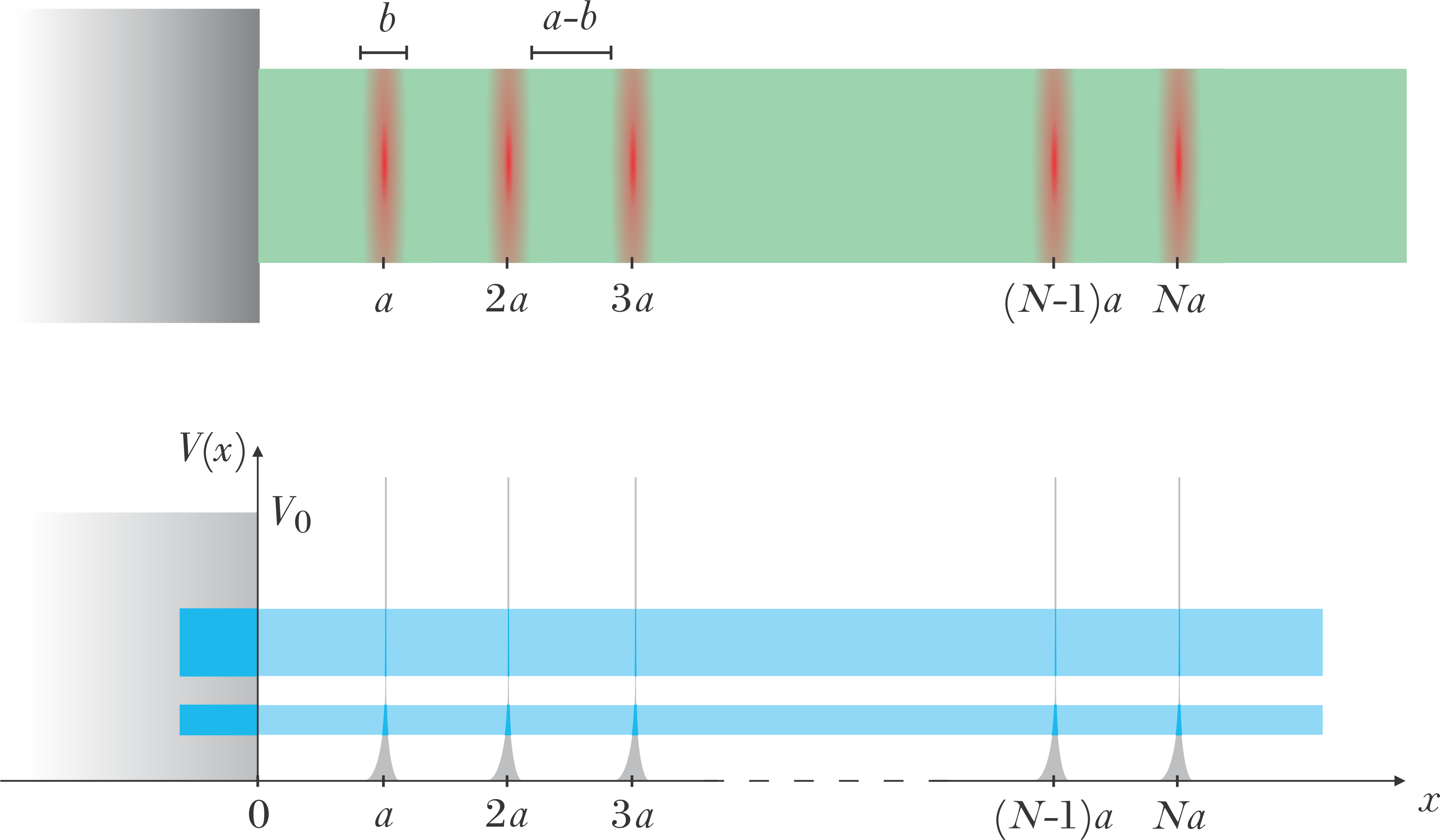
Figure 1: (Color online) The upper figure illustrates a locally periodic system composed by two media, blocked at the left. It represents an elastic system, a microwave waveguide, a one-dimensional photonic crystal, or a superlattice. The lower figure is a schematic representation of the potential function in the corresponding quantum case, where the first sub-bands are shown as blue fringes.

Here, we provide a physical multiple-scattering setting that leads to an exact analytical expression for the optical $S$ matrix. This expression appears in the thermodynamic or large size limit as the number of scatterers $N\rightarrow\infty$. For locally periodic structures the scattering process has been shown to be analogous to a nonlinear dynamical evolution such that the scattering matrix gradual change with size is equivalent to iteration of a dissipative mapping that displays transitions to chaos of the tangent bifurcation type MR ; VictorJOPA ; MDR . The transitions from localized to extended states correspond to transitions from regularity to chaos MR ; VictorJOPA ; MDR and the chaotic regimes hold an ergodic property Schuster .

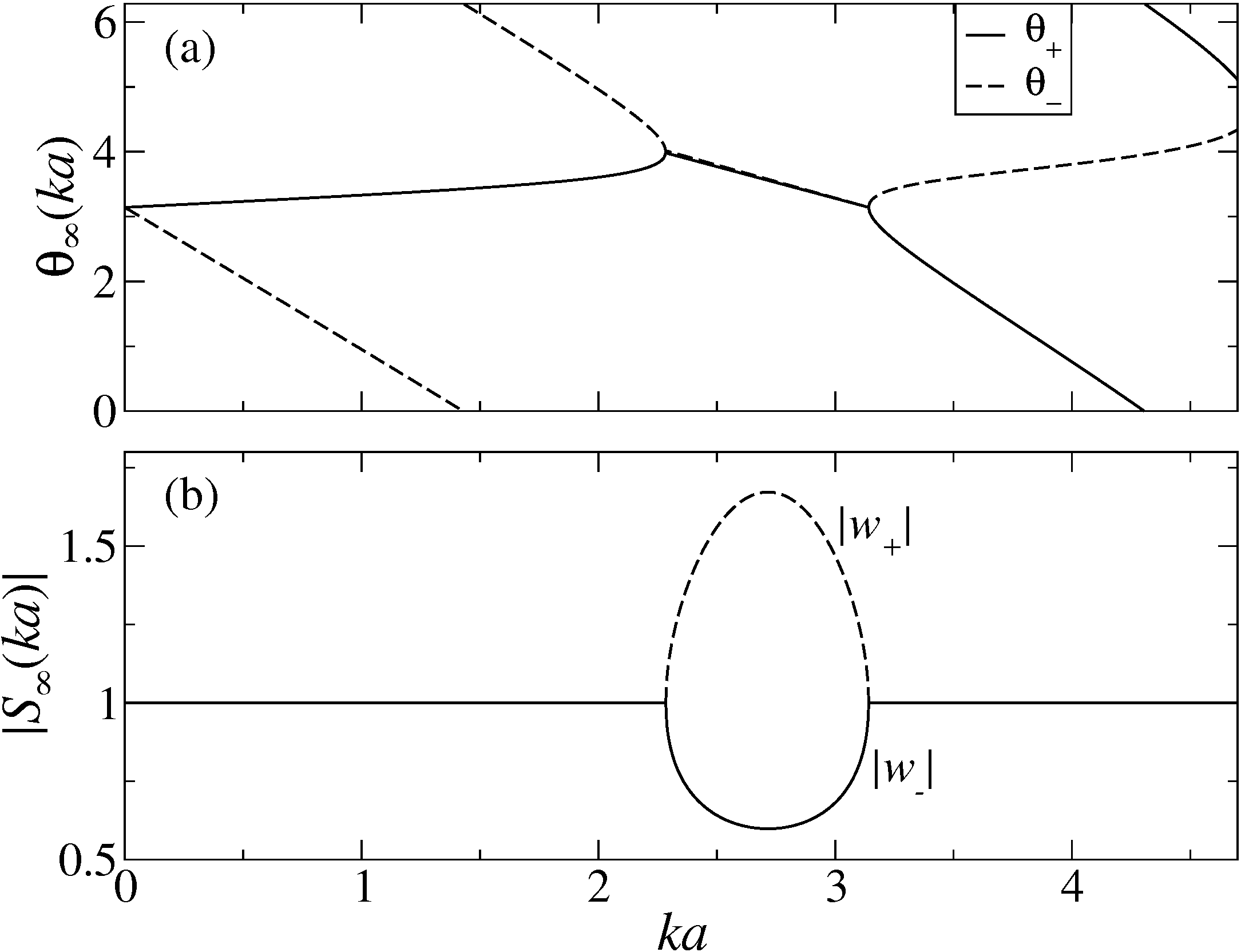
Figure 2: Fixed point solutions $S_{\infty}(ka)$, Eqs. (2)-(4), (a) phase and (b) modulus. The phases of $w_{+}$ and $w_{-}$ are the same within the gaps but the stable solutions are $\theta_{+}(ka)$ or $\theta_{-}(ka)$ depending on the gap defined by the values of $ka$. Note that $|w_{+}(ka)|>1$ while $|w_{-}(ka)|<1$ within the band.

Let us consider a single port quantum system in one dimension, as shown in Fig. 1; it consists of a periodic array with a finite number of identical scattering elements Griffiths ; Morales ; Luna . The system with $N-1$ scatterers is described by the $1\times 1$ scattering matrix $S_{N-1}$, and this can be immediately related to the scattering matrix $S_{N}$ of a system with $N$ scatterers by addition of another scatterer. The result is the recurrence relation  VictorJOPA

$$S_{N}=\frac{r^{\prime}_{b}z_{b}^{*}+z_{b}S_{N-1}}{{r^{\prime}_{b}}^{*}z_{b}+z_{b}^{*}S^{*}_{N-1}}S^{*}_{N-1},$$ (1)

where $r_{b}$ ($t_{b}$) and $r^{\prime}_{b}$ ($t^{\prime}_{b}$) are the reflection (transmission) amplitudes of an individual scatterer for incidence on the left and right, respectively; $z_{b}=t_{b}\mathrm{e}^{\mathrm{i}\phi/2}\mathrm{e}^{\mathrm{i}k(a-b)}$, with $\mathrm{e}^{\mathrm{i}\phi/2}=t^{\prime}_{b}/t_{b}$, $k$ is the incident wave number, $b$ the width of the scatterer, and $a$ the lattice constant. Since $S_{N}$ depends intrinsically on $k$, a gap and band structure emerges with respect to $k$ as $N$ increases (see below). The gaps and bands are clearly formed in the thermodynamic limit $N\rightarrow\infty$, for which Eq. (1) has a stable and an unstable fixed point solutions for each value of $k$; these are VictorJOPA

$$S_{\infty}(k)=\left\{\begin{array}[]{ll}\mathrm{e}^{\mathrm{i}\theta_{\pm}(k)},&k\in\,\mbox{gap}\\ w_{\pm}(k),&k\in\,\mbox{band},\end{array}\right.\,$$ (2)

where

$$\mathrm{e}^{\mathrm{i}\theta_{\pm}(k)}=\frac{\pm\sqrt{\left[\mathrm{Re}\,z_{b}(k)\right]^{2}-\left|t_{b}(k)\right|^{4}}+\mathrm{i}\,\mathrm{Im}\,z_{b}(k)}{r_{b}^{*}(k)z_{b}(k)},$$ (3)

and

$$w_{\pm}(k)=\mathrm{i}\,\frac{\pm\sqrt{\left|t_{b}(k)\right|^{4}-\left[\mathrm{Re}\,z_{b}(k)\right]^{2}}+\mathrm{Im}\,z_{b}(k)}{r_{b}^{*}(k)z_{b}(k)}\,.$$ (4)

These solutions are shown in Fig. 2.

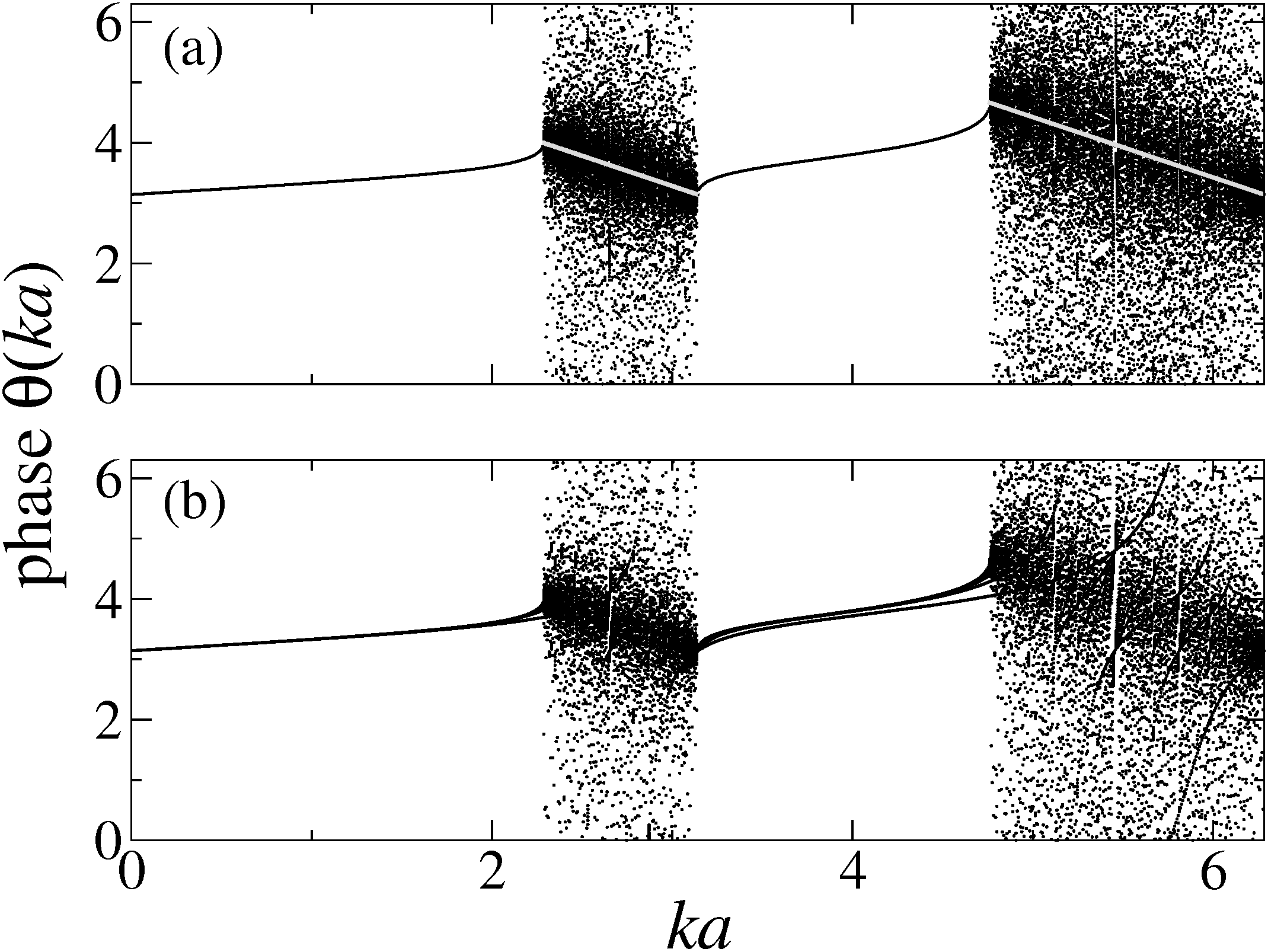
Figure 3: Phase $\theta$ of the scattering matrix as a function of incident energy $ka$. In (a) we plot the last 30 of 1000 iterations of the recurrence relation Eq. (1) and also the analytical expression for the stable solution of Eq. (2) (see Fig. 2). The stable solution is indistinguishable from the numerical result within the gaps, while it gives the maximum of the distribution of the phase within the bands (light line). See Fig. 4. In (b) we show the evolution of the phase from $N=1$ up to $N=30$, where the additional black lines are transient values associated with the unstable (repellor) solutions.

The recurrence relation Eq. (1) for the (complex number) scattering matrix $S_{N}$ is also a recurrence relation for the phase $\theta_{N}$, $S_{N}=\exp(\mathrm{i}\theta_{N})$, which can be interpreted as a real number nonlinear iterated map. The main features of this map, including its generalization to Bethe lattice arrangements of scatterers, have been determined in Refs. MR ; VictorJOPA ; MDR . It was found that the bifurcation diagram, or families of attractors ordered according to the control parameter $ka$, is made of intervals of regular attractors of period 1 separated by sectors of chaotic attractors. The attractors at the boundaries between the two kinds of families are transitions to chaos of the tangent bifurcation type Schuster . The chaotic attractors in the vicinity of the tangent bifurcations exhibit intermittency of type I Schuster . Therefore the gap and band behavior of the scattering system in Fig. 3(a) is actually the map bifurcation diagram in the language of the dynamical system analog.

When $N\rightarrow\infty$ the value $S_{\infty}$ of the scattering matrix is fixed within the gaps and given by the complex number of modulus 1 in Eq. (2). The value of the scattering matrix fluctuates within the bands, but, as we shall conclude shortly, its average value $\langle S\rangle$ is fixed by the non unitary complex number $S_{\infty}$ in Eq. (2), see Fig. 2. From Eq. (1) we observe that

$$\lim_{N\to\infty}S_{N}^{m}=\left(\lim_{N\to\infty}S_{N}\right)^{m}=S_{\infty}^{m},$$ (5)

with $m$ an integer. This property coincides with the analyticity condition satisfied by the average of the scattering matrix MelloLesHouches . The scattering matrix visits its available space according to a certain distribution fixed by the value of $ka$ within the bands. This distribution becomes specified since the analyticity condition, expressed in Eq. (5), implies that all of its moments are known; the resulting distribution is given by Poisson’s kernel MelloBook ; LMS ; MelloLesHouches , namely

$$p_{\langle S\rangle}(S)=\frac{1}{2\pi}\,\frac{\left|1-\left|\left\langle S\right\rangle\right|^{2}\right|}{\left|S-\left\langle S\right\rangle\right|^{2}},\quad\mbox{with}\quad\langle S\rangle=S_{\infty},$$ (6)

where the absolute value in the numerator was added to ensure a positive defined distribution for the case of an over unitary value $\langle S\rangle=w_{+}(ka)$. Thus, $p_{\langle S\rangle}(S)$ depends on $k$ through the reflection and transmission amplitudes of a single scattering element, Eqs. (3), and (4).

The results in Eqs. (5) and (6) are anticipated MelloBook ; LMS ; MelloLesHouches to be of general validity and can be corroborated by considering the nonlinear map analogs of the scattering processes described here and in Refs. MR ; VictorJOPA ; MDR . The chaotic dynamics within the bands formed by these model systems are ergodic and ensure the existence of an invariant distribution $P(\theta)$ (actually, the distribution for the phase $\theta$). That is, iteration time averages for map trajectories within the chaotic attractors are reproduced by ensemble averages. The identification of $p_{\langle S\rangle}(S)$ with the Poisson kernel and of $S_{\infty}$ with $\langle S\rangle$ is accomplished by determination of $P(\theta)$ and its average.

The quantum chain of delta potentials shown in the lower part of Fig. 1 will be used as a specific example VictorJOPA . To obtain a $1\times 1$ scattering matrix it is necessary that energy of the particle is smaller than the height $V_{0}$ of the step potential on the left side of the chain. In this case $r_{b}=r^{\prime}_{b}=-u/(u-2\mathrm{i}k)$ and $t_{b}=t^{\prime}_{b}=-2\mathrm{i}k/(u-2\mathrm{i}k)$, with $u$ the intensity of the delta potential in the same units as the wave number. We take the initial condition $S_{0}=\mathrm{e}^{\mathrm{i}\pi}$, which corresponds to $V_{0}\to\infty$. In Fig. 3 the phase of the scattering matrix is plotted for $ua=10$ as a function of $ka$ (dimensionless quantities are used). In Fig. 3(a) the last 30 of 1000 iterations are plotted, as well as the fixed point solution (we show only the stable solution) which is highlighted in the bands but it is indistinguishable from the numerical result within the gaps. In Fig. 3(b) the first 30 iterations show the distribution of points around a maximum value given by the fixed point solution.

The numerically-obtained distributions for the phase $P(\theta)$ from an ensemble of $N=10^{4}$ scattering systems are shown as histograms in Fig. 4 for several values of $k$. In Fig. 4(a) we observe that, for $k$ within the first gap, the distribution is just a delta function centered at the stable fixed point solution. The fixed point solution is exponentially reached as $N$ approaches the limit $N\to\infty$ VictorJOPA . A similar outcome happens for the unstable fixed point solution in which the phase remains there for all $N$. In contradistinction, for $k$ inside, starting close to the border of the band and progressively at values further inside the band, panels (b), (c) and (d) of Fig. 4, respectively, the phase $\theta$ of $S$ becomes distributed in the complete space between 0 and $2\pi$. Near the transition from gap to band the distribution is narrower than that for $k$ close to the center of the band. At the gap/band transition the fixed point solution is reached as a power law VictorJOPA . In all of the cases shown, the histograms have an excellent agreement with the Poisson kernel (6) for $\langle S\rangle$ calculated from Eqs. (2) with $S_{\infty}=\langle S\rangle$, as well as when it is calculated from the numerical data. This excellent agreement shows that $S_{\infty}$ is the optical $S$ matrix.

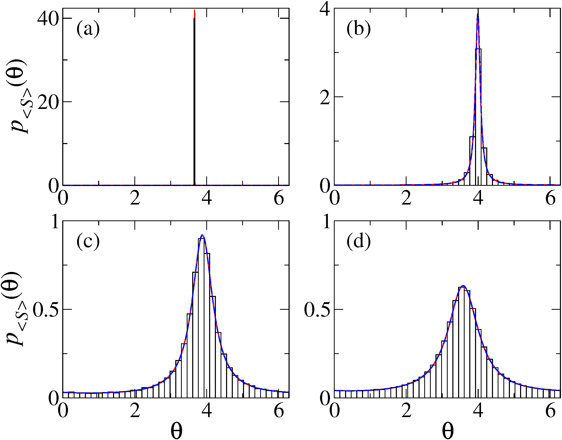
Figure 4: Distribution of the phase for $N=10^{4}$ iterations of the recurrence relation, Eq. (1), for a chain of delta potentials with intensity $ua=10.0$ and initial condition $\theta_{0}=\pi$. The histograms are obtained at fixed $k$: (a) $ka=2.1$, (b) $ka=2.29$, (c) $ka=2.4$, and (d) $ka=2.7$. The dashed lines (blue lines) correspond to the theoretical model of Eq. (6) in which the average is given by $\langle S\rangle=S_{\infty}$. Although we show only results for the stable fixed point solutions $w_{-}$ the same theoretical distribution holds for the unstable solution $w_{+}$. The continuous lines (red lines) also correspond to Eq. (6) but $\langle S\rangle$ is obtained from the numerical data.

In conclusion, an analytical expression for the average of the scattering matrix, known as the optical $S$ matrix in the nuclear physics terminology, was calculated for the first time. This was done by demonstrating that the fixed point solution $N\rightarrow\infty$ of the size recurrence relation of the scattering matrix, for a locally periodic system, satisfies the analyticity condition. When $N\rightarrow\infty$ a perfect crystal, with consecutive gaps and bands, or localized and extended states, is obtained as the incident energy $ka$ is increased. There is a precise analog of the scattering problem with a nonlinear (dissipative) iterated map, such that the gap and bands of the scattering system correspond, respectively, to the regular and chaotic attractors in the nonlinear dynamics. The boundaries between corresponding to transition from localized to extended states can be identified with transitions in or out of chaos of the tangent bifurcation kind. A complete transcription from the two languages can be established, such that, for instance, the vanishing of the Lyapunov exponent at the transitions to chaos corresponds to the divergence of the localization length at the gap to band boundaries. The nonlinear map exhibits two types of dynamical properties: those of trajectories towards the attractor and those inside the attractor. In the former case the number of iterations corresponds to the number of scatterers $N$, and therefore describes system size growth. In the latter case map iterations have a different meaning. For a regular attractor, period one in our example, iterations only repeat certain values of the map variable, in our example iterations keep the phase and the scattering matrix at their constant fixed-point values, $\theta_{\infty}$ and $S_{\infty}=\exp(\mathrm{i}\theta_{\infty})$. For the chaotic attractors iterations change repeatedly the value of the map variable sampling the space spanned by the attractor, in our example the phase $\theta$ interval $[0,2\pi]$, according to a given distribution, the invariant distribution. The chaotic attractors that appear for given intervals of the control parameter $k$ possess the ergodic property, such that iteration time averages are equal to invariant distribution averages. The invariant distribution is identified as the distribution of the phase $P(\theta)$ in the $N\rightarrow\infty$ limit. In this limit the average of the scattering matrix $\langle S\rangle$, the optical $S$ matrix is equal to the fixed point value $S_{\infty}$. This was verified by using the fixed point solution in the expression of Poisson’s kernel for $P(\theta)$. The theoretical distribution fits perfectly the histogram obtained from numerical iterations for a chain of delta potentials. The same is valid when the optical $S$ matrix is obtained from the numerical average of the scattering matrix.

I Acknowledgements

This work was supported by DGAPA-UNAM under project IN103115. We thank Centro Internacional de Ciencias for the facilities given for several group meetings and gatherings celebrated there. VD-R thanks the financial support of DGAPA. A. Robledo acknowledges support from DGAPA-UNAM-IN104417. We thank G. Báez, J. A. Méndez-Bermúdez, and A. M. Martínez-Argüello for useful comments.

References

- (1) R. G. Newton, Scattering theory of waves and particles (Dover Publications, 2nd ed., New York, 2013).
- (2) K. S. Krane, Introductory nuclear physics (John Wiley & Sons, Inc., Hoboken, 1988).
- (3) P. A. Mello and N. Kumar, Quantum Transport in Mesoscopic Systems: Complexity and Statistical Fluctuations (Oxford University Press, New York, 2005).
- (4) R. Landauer, Phil. Mag. 21, 863 (1970).
- (5) M. Büttiker, Y. Imry, R. Landauer, and S. Pinhas, Phys. Rev. B 31, 6207 (1985).
- (6) M. Büttiker, J. Phys.: Condens. Matter 5, 9361 (1993).
- (7) P. W. Brouwer, S. A. van Langen, K. M. Frahm, M. Büttiker, C. W. J. Beenakker, Phys. Rev. Lett. 79, 913 (1997).
- (8) P. W. Brouwer, Phys. Rev. B 58, R10135 (1998).
- (9) E. Doron, U. Smilansky, and A. Frenkel, Phys. Rev. Lett. 65, 3072 (1990).
- (10) H. Schanze, E. R. P. Alves, C. H. Lewenkopf, and H.-J. Stöckmann, Phys. Rev. E 64, 065201(R) (2001).
- (11) R. A. Méndez-Sánchez, U. Kuhl, M. Barth, C. H. Lewenkopf, and H.-J. Stöckmann, Phys. Rev. Lett. 91, 174102 (2003).
- (12) S. Hemmady, X. Zheng, E. Ott, T. M. Antonsen, and S. M. Anlage Phys. Rev. Lett. 94, 014102 (2005).
- (13) E. Flores-Olmedo, A. M. Martínez-Argüello, M. Martínez-Mares, G. Báez, J. A. Franco-Villafañe, and R. A. Méndez-Sánchez, Sci. Rep. 6, 25157 (2016).
- (14) S. E. A. Orrigo, H. Lenske, F. Cappuzzello, A. Cunsolo, A. Foti, A. Lazzaro, C. Nociforo, and J. S. Winfield, Phys. Lett. B 633, 469 (2006).
- (15) K. M. Watson, Phys. Rev. 89, 575 (1953).
- (16) L. Silvestri, G. J. Kalman, Z. Donkó, P. Hartmann, and H. Kählert, EPL 109, 15003 (2015).
- (17) M. W. Keller, A. Mittal, J. W. Sleight, R. G. Wheeler, D. E. Prober, R. N. Sacks, and H. Shtrikmann, Phys. Rev. B 53, R1693 (1996).
- (18) C. M. Marcus, A. J. Rimberg, R. M. Westervelt, P. F. Hopkins, and A. C. Gossard, Phys. Rev. Lett. 69, 506 (1992).
- (19) M. I Tribelsky, S. Flach, A. E. Miroshnichenko, A. V. Gorbach, and Y. S. Kivsha, Phys. Rev. Lett. 100, 043903 (2008).
- (20) U. Kuhl, M. Martínez-Mares, R. A. Méndez-Sánchez, and H.-J. Stöckmann, Phys. Rev. Lett. 94, 144101 (2005).
- (21) H. Schanze, H.-J. Stöckmann, M. Martínez-Mares, and C. H. Lewenkopf, Phys. Rev. E 71, 016223 (2005).
- (22) M. Lawniczak, S. Bauch, O. Hul, and L. Sirko, Phys. Scr. T147, 014018 (2012).
- (23) A. M. Martínez-Argüello, M. Martínez-Mares, M. Cobián-Suárez, G. Báez, and R. A. Méndez-Sánchez, EPL 110, 54003 (2015).
- (24) G. López, P. A. Mello, and T. H. Seligman, Z. Phys. A 302, 351 (1981).
- (25) Theory of random matrices: spectral statistics and scattering problems. P. A. Mello in Mesoscopic quantum physics, edited by E. Akkermans, G. Montambaux, J.-L. Pichard, and J. Zinn-Justin (North-Holland, Amsterdam, 1995), p. 465.
- (26) P. A. Mello, P. Pereyra, and T. H. Seligman, Ann. Phys. (N. Y.) 161, 254 (1985).
- (27) M. Martínez-Mares and A. Robledo, Phys. Rev. E 80, 045201 (2009).
- (28) V. Domínguez-Rocha and M. Martínez-Mares, J. Phys. A: Math. Theor. 46, 235101 (2013).
- (29) M. Martínez-Mares, V. Domínguez-Rocha, and A. Robledo, Eur. Phys. J. Special Topics 226, 417 (2017).
- (30) H.G. Schuster, Deterministic Chaos. An Introduction. 2nd ed. Weinheim: Wiley-VCH, 1988
- (31) D. J. Griffiths and C. A. Steinke, Am. J. Phys. 69, 137 (2001).
- (32) A. Morales, J. Flores, L. Gutiérrez, and R. A. Méndez-Sánchez, J. Acoust. Soc. Am. 112, 1961 (2002).
- (33) G. A. Luna-Acosta, H. Schanze, U. Kuhl, and H.-J. Stöckmann, New J. Phys. 10, 043005 (2008).