Chiral plasmon in gapped Dirac systems

Abstract

We study the electromagnetic response and surface electromagnetic modes in a generic gapped Dirac material under pumping with circularly polarized light. The valley imbalance due to pumping leads to a net Berry curvature, giving rise to a finite transverse conductivity. We discuss the appearance of nonreciprocal chiral edge modes, their hybridization and waveguiding in a nanoribbon geometry, and giant polarization rotation in nanoribbon arrays.

Introduction— The Berry curvature is a topological property of the Bloch energy band, and acts as an effective magnetic field in momentum spaceBerry (1984); Xiao et al. (2010); Nagaosa et al. (2010). Hence, topological materials may exhibit anomalous Hall-like transverse currents in the presence of an applied electric field, in absence of a magnetic field. Examples includes topological insulatorsHasan and Kane (2010) with propagating surface states that are protected against backscattering from disorder and impurities, and transition metal dichalcogenides where the two valleys carry opposite Berry curvature giving rise to a bulk topological charge neutral valley currentsXiao et al. (2012); Mak et al. (2014). These bulk topological currents were also experimentally investigated in other Dirac materials, such as gapped graphene and bilayer graphene systemGorbachev et al. (2014); Sui et al. (2015). The electromagnetic response of these gapped Dirac systems, particularly that due to its surface electromagnetic modes (i.e plasmons) are relative unexplored.

In gapped graphene or transition metal dichalcogenides, electrons in the two valleys have opposite Berry curvature, ensured by time-reversal symmetry (TRS) of their chiral HamiltoniansXiao et al. (2012). Hence, far field light scattering properties of these system does not differentiate between circularly polarized light, i.e. zero circular dichroism in the classical sense. Optical pumping with circularly polarized light naturally breaks TRS, and a net chirality ensues. However, under typical experimental conditions, the transverse conductivity due to Berry curvature is less than the quantized conductivity $e^{2}/\hbar$, and the associated optical dichroism effect is not prominent. These effects, however, can potentially be amplified through enhanced light-matter interaction with plasmonsGrigorenko et al. (2012); Koppens et al. (2011); Jablan et al. (2009); Low and Avouris (2014); Giuliani and Vignale (2005).

In this letter, we discuss the emergence of new chiral electromagnetic plasmonic modes and their associated optical dichroism effect. We consider a gapped Dirac system under continuous pumping with cicularly polarized light. We discuss the appearance of edge chiral plasmons, and how they can allow launching of one-way propagating edge plasmons in a semi-infinite geometry. We consider also the hybridization of these chiral edge modes in a nanoribbon geometry and the possibility of nonreciprocal waveguiding. Their far-field optical properties reveal resonant absorption accompanied by sizeable polarization rotation.

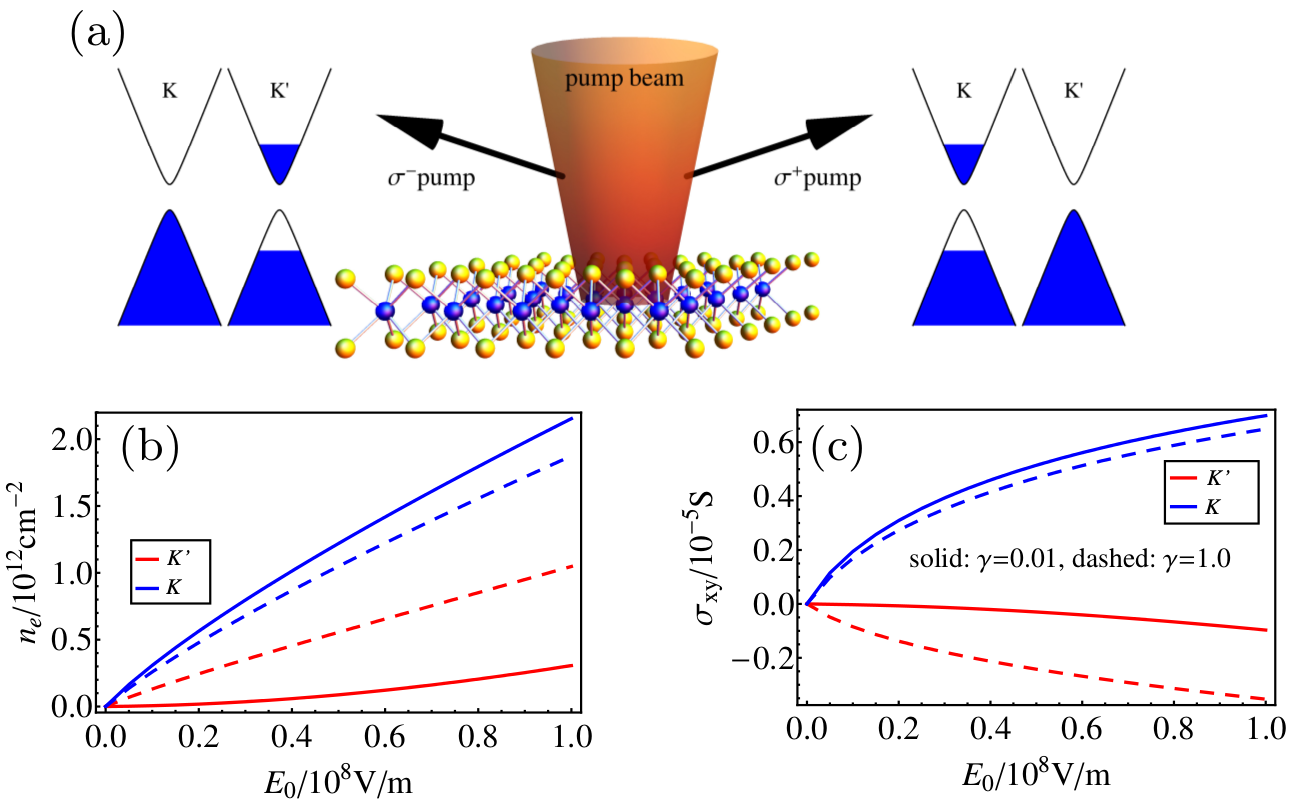
Figure 1: Optically induced valley polarization: (a) Polarization selective pumping leads to different populations in the $K$ and $K^{\prime}$ valleys. (b) DC electronic carrier concentration in the two valleys as a function of the pump electric field. (c) DC $\sigma_{xy}$ in the two valleys as a function of the right circular polarized pump electric field

Model system— We consider the following Hamiltonian of a massive Dirac system (MDS),

$${\cal H}=\hbar v_{f}\mathbf{k}\cdot\bm{\sigma}_{\tau}+\tfrac{\Delta}{2}\sigma_{z}$$ (1)

where $\bm{\sigma}_{\tau}=(\tau\sigma_{x},\sigma_{y})$, $\tau=\pm 1$ denotes the $\mathbb{K}$/$\mathbb{K^{\prime}}$ valley, $\Delta$ is the energy gap and $v_{f}$ is the Fermi velocity. We denote the eigenenergy and wavefunctions of ${\cal H}$ as ${\cal E}_{\tau,\nu}(\mathbb{k})$ and $\Psi_{\tau,\nu}(\mathbb{k})$, with $\nu=c,v$ denoting the electron and hole bands. We are interested in the dynamics of the electronic subsystem in an external electromagnetic field $\mathbb{E}$ as illustrated in Fig. 1a, which can be described with the von Neumann equation, $i\hbar\,\partial_{t}\hat{\rho}=[{\cal H}+V,\hat{\rho}]$, where $\hat{\rho}$ is the statistical operator of the electron subsystem and $V=-e\mathbb{E}\cdot\mathbb{r}$ is the interaction term. In the $\Psi_{\tau,\nu}(\mathbb{k})$ basis, the equation of motion is written explicitly asSlepyan et al. (2004); Nemilentsau et al. (2006),

$$\frac{\partial\rho_{jj^{\prime}}}{\partial t}+\frac{e}{\hbar}\mathbb{E}\cdot\frac{\partial\rho_{jj^{\prime}}}{\partial\mathbb{k}}=-\frac{i}{\hbar}\rho_{jj^{\prime}}[{\cal E}_{j}(\mathbb{k})-{\cal E}_{j^{\prime}}(\mathbb{k})]$$

$$+\frac{ie}{\hbar}\mathbb{E}\cdot\sum_{j^{\prime\prime}}\left[\mathbb{R}_{jj^{\prime\prime}}(\mathbb{k})\rho_{j^{\prime\prime}j^{\prime}}-\rho_{jj^{\prime\prime}}\mathbb{R}_{j^{\prime\prime}j^{\prime}}(\mathbb{k})\right]$$ (2)

where $[\rho(t,\mathbb{k})]_{j,j^{\prime}}$ is the density matrix, $\mathbb{R}_{jj^{\prime}}(\mathbb{k})=(i/2)\int\Psi_{j}^{*}(\mathbb{k})\partial_{\mathbf{k}}\Psi_{j^{\prime}}(\mathbb{k})d\mathbb{r}+hc$, with $j=\{\nu,\tau\}$ designating quantum number of electrons. In Eq. (Chiral plasmon in gapped Dirac systems) we neglect indirect interband optical transitions.

Here, we are interested in the interaction with a continuous (c.w.) monochromatic electromagnetic wave, $\mathbb{E}=\mathbb{E}_{0}e^{-i\omega t}+cc$. Using the rotating wave approximation and introducing relaxation phenomenologically within the relaxation time approximation, we obtain the steady-state solution as a system of four linear equations for diagonal components of the distribution function, $\rho_{j}\equiv\rho_{jj}$,

$$\rho_{\nu,\tau}(\mathbb{k})=\beta_{\tau}\left(\rho_{\nu,\tau}^{0}(\mathbb{k})+\gamma\rho_{\nu,\tau^{\prime}}(\mathbb{k})+\alpha_{\tau}\rho_{\nu^{\prime},\tau}(\mathbb{k})\right)$$ (3)

where $\tau^{\prime}\neq\tau$ and $\nu^{\prime}\neq\nu$. Here,

$$\alpha_{\tau}=\frac{2e^{2}|\mathbb{E}_{0}\cdot\mathbb{R}_{cv}^{\tau}(\mathbb{k})|^{2}}{\hbar^{2}\left[(\omega-\omega_{cv})^{2}+1/\tau_{0}^{2}\right]},$$ (4)

$\omega_{cv}=({\cal E}_{\tau,c}-{\cal E}_{\tau,v})/\hbar$, $\beta_{\tau}=1/(1+\gamma+\alpha_{\tau})$, $\gamma=\tau_{0}/\tau_{1}$, where $\tau_{0}$ is the population relaxation time and $\tau_{1}$ is the intervalley scattering time (see supplementary information). The equilibrium distribution function is given by the Fermi Dirac distribution, $\rho_{\nu,\tau}^{0}(\mathbb{k})=[1+\mbox{exp}(({\cal E}_{\tau,\nu}(\mathbb{k})-\mu)/k_{B}T)]^{-1}$.

Let us consider positive or right circular polarized light, $\mathbf{E}_{0}=E_{0}\left(\mathbf{e}_{x}+i\mathbf{e}_{y}\right)$, interacting with electrons at the top of valence band, $\mathbf{R}_{cv}^{\tau}(\mathbf{0})=-(v_{f}\hbar/\Delta)\left(i\tau\mathbf{e}_{x}+\mathbf{e}_{y}\right)$. It can be clearly seen that $\mathbb{E}_{0}\cdot\mathbb{R}_{cv}^{\tau}(\mathbf{0})=-i(v_{f}\hbar/\Delta)(\tau+1)$, and thus $\alpha_{\tau}$, are zero at $\mathbf{K}^{\prime}$ valley while being finite at the $\mathbb{K}$ valley. Hence, pumping with circularly polarized light would lead to carrier population imbalance between the two valleys.

Net chirality with pumping— The effective Hamiltonian in Eq. 1 captures the valley physics in physical system such as monolayer graphene with staggered sublattice potentialNeto et al. (2009) and transition metal dichalcogenidesXiao et al. (2012), if the spin-orbit coupling term can be neglected. To proceed, we consider some reasonable numbers for our model gapped Dirac system; an energy gap $\Delta=0.5$eV and Fermi velocity $v_{f}=1\times 10^{6}\,$ms^-1. Our calculations assume temperature $T=300\,$K, typical carrier lifetimes $\tau_{0}=1\,$ps and that the system is undoped at equilibrium. With pumping, charge neutrality and electron-hole symmetry would require that the electron and hole carrier densities follow $n_{e}^{\tau}=n_{h}^{\tau}$. Fig. 1b shows the increasing non-equilibrium electron densities as function of pump intensities $E_{0}$, under continuous wave pumping with right circular polarized light. Finite transfers of electrons from the $\mathbb{K}$ to $\mathbb{K}^{\prime}$ valley is determined by the inter-valley scattering rate described by $\gamma$.

In the presence of an external electric field $\mathbb{E}$, the carrier velocity acquires a non-classical transverse term due to Berry curvature, $\bm{\Omega}_{\tau}(\mathbb{k})$, given by $-\tfrac{e}{\hbar}\mathbb{E}\times\bm{\Omega}_{\tau}(\mathbb{k})$. For a MDS, the form of the Berry curvature is well knownXiao et al. (2012). Within the semiclassical Boltzmann transport theory, this would give rise to a transverse conductivity, which in the charge neutral case we are considering here is simply given by $\sigma^{\tau}_{xy}=2e^{2}/\hbar\int[d\mathbb{k}]\rho_{c,\tau}(\mathbb{k})\Omega_{\tau}(\mathbb{k})$. The factor of $2$ accounts for contributions from both electrons and holes. It can further be shown that $\sigma^{\tau}_{xy}=-\sigma^{\tau}_{yx}$. Since TRS requires $\Omega_{\mathbb{K}}(\mathbb{k})=-\Omega_{\mathbb{K}^{\prime}}(\mathbb{k})$, $\sigma^{\mathbb{K}}_{xy}=-\sigma^{\mathbb{K}^{\prime}}_{xy}$ at equilibrium. However, under continuous wave pumping, the asymmetric carrier populations in the two valleys would produce a net transverse conductivity, as shown in Fig. 1c. We note that over the frequency range that we are interested in, i.e. $\hbar\omega\ll\Delta$, $\sigma_{xy}$ is real and frequency independentLi and Carbotte (2012). Our calculations suggest that $\sigma_{xy}$ an order smaller than $e^{2}/\hbar$ is obtainable with pump intensities $E_{0}$ routinely used in pump-probe experiments. The non-equilibrium longitudinal components of the conductivity, $\sigma_{xx}=\sigma_{yy}$, are computed with the Kubo formulaLi and Carbotte (2012). For all the subsequent results of this paper, we use a pump intensity of $E_{0}=10^{8}$ V/m and $\gamma=0.01$.

Valley induced bulk and edge chiral plasmon— Armed with the conductivity sum of the two valleys, $\sigma_{ij}$ we discuss general results for the plasmon modes in this system. Plasmon dispersion in a continuous sheet of the MDS is given byChiu and Quinn (1974); Hanson (2008); Yudin et al. (2015):

$$\left[\frac{\epsilon_{1}}{\kappa_{1}}+\frac{\epsilon_{2}}{\kappa_{2}}+\frac{\imath\sigma_{xx}}{\omega\epsilon_{0}}\right]\cdot\left[\kappa_{1}+\kappa_{2}-\frac{\imath\sigma_{yy}}{c\epsilon_{0}}k_{0}\right]-\frac{\sigma_{xy}\sigma_{yx}}{(c\epsilon_{0})^{2}}=0$$ (5)

where $\kappa_{1,2}=\sqrt{q^{2}-\epsilon_{1,2}k_{0}^{2}}$ are the evanescent decay constants on either side of the 2D sheet. As shown in Fig. 2, this “bulk plasmon” dispersion is symmetric with respect to the wavevector $q$, since it appears quadratically in Eq. 5.

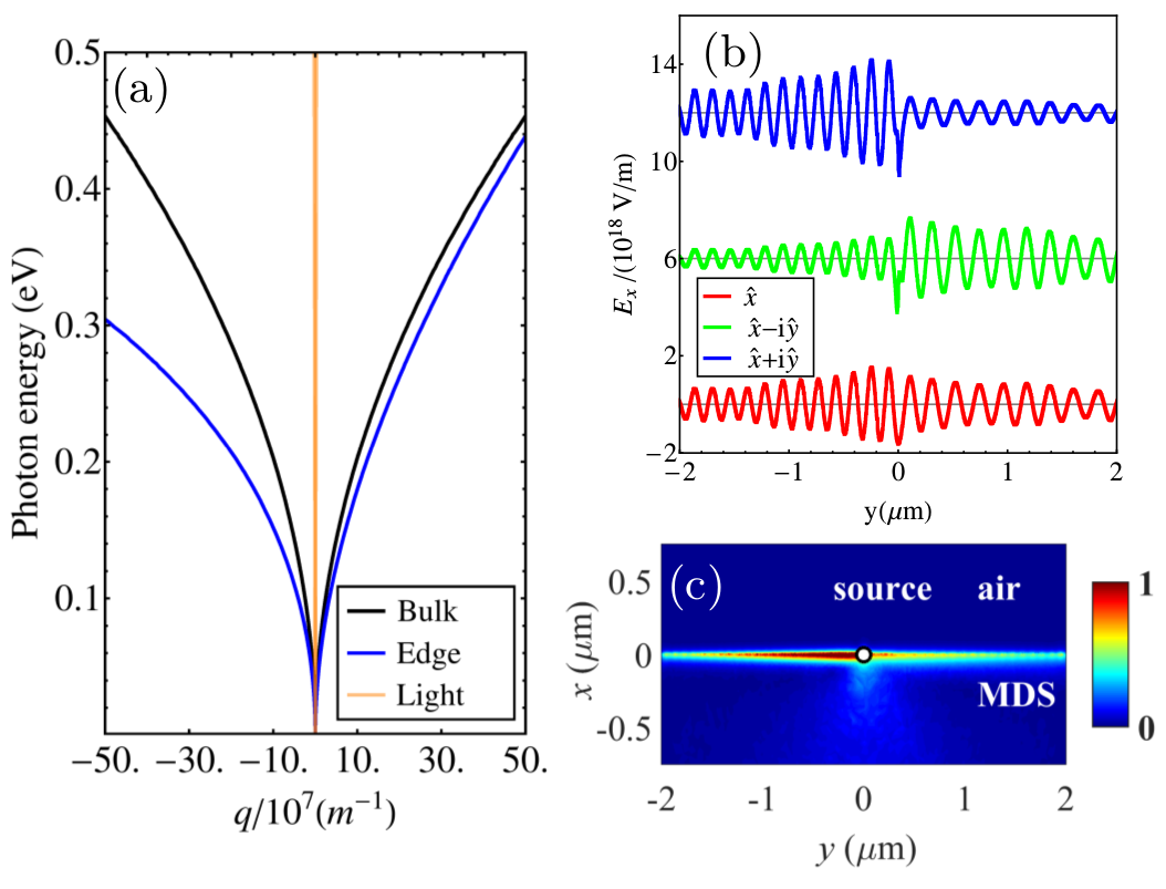
Figure 2: (a) Chiral plasmon dispersion in bulk and semi-infinite MDS. (b) Selective excitation of edge modes using circular and linear polarized dipoles placed at the origin: Line plots of electric field $E_{x}$ in the plane and perpendicular to the edge. The vertical offset is $6\times 10^{18}$V/m. (c) $|E|$ field (normalized to max) profile for a $\hat{x}$-polarized emitter located near the edge of semi infinite Dirac material ($x<0$) at $\omega=$0.1\text{\,}\mathrm{e}\mathrm{V}$$. Both of these field profiles show nonreciprocal emission into the edge mode. The dipoles are placed $10\text{\,}\mathrm{n}\mathrm{m}$ above the MDS.

Edges can also accommodate plasmon modesFetter (1985). Symmetry arguments show that although bulk plasmon dispersion respects $\omega(\mathbf{q})=\omega(-\mathbf{q})$ with nonsymmetric conductivity tensor, the presence of an edge can break this degeneracyCamley (1987). Here we consider the case of semi-infinite MDS. Within the quasistatic picture, the edge plasmon dispersion is approximately given byFetter (1985); Wang et al. (2012): $\eta^{2}-\chi^{2}-3\eta+2\sqrt{2}\chi\mathop{\mathrm{sgn}}(q)=0$, where $\eta=|q|\sigma_{xx}/(\imath\epsilon_{0}\epsilon\omega)$ and $\chi=|q|\sigma_{xy}/(\epsilon_{0}\epsilon\omega)$. Fig. 2a indeed shows that the right moving edge plasmon has a different dispersion compared to the left moving one. A simple realization of this nonreciprocity effect consists of placing a dipole near the edge of the material. Finite element simulation of near field dipole emission was performed using comsol. As shown in Fig. 2b and c, the linear dipole preferentially emits into the left propagating edge state. Taking a cue from le Feber et al. (2015), we can also use a circular dipole to couple emission into left or right edge state, depending on dipole helicity. The results for circular dipoles are presented in Fig. 2b.

In terms of experiment, the appropriate plasmon momentum can be selected either by use of a grating near the edgeRaether (1988), by adjusting the distance between the tip of a near field microscope and the edge of the MDS or the tip radiusFei et al. (2011, 2012); Chen et al. (2012). Since the edge plasmon dispersion is nonreciprocal, selection of the magnitude of the plasmon momentum will also lead to selectivity in the propagation direction. In addition to the different intensities of the two, the different wavelengths for the left and right moving edge modes in this configuration might be used for nonreciprocal phase shiftersSounas and Caloz (2011).

Waveguiding in nanoribbons– Any practical realization of the semi-infinite case discussed above will involve a stripe or waveguide geometry. Waveguides are an important component of plasmonic circuitryFang and Sun (2015) and ribbon waveguides based on the plasmon modes in graphene have been proposedNikitin et al. (2011); Christensen et al. (2012). In this section, we show how the chirality of the plasmon leads to the propagation direction being coupled to the ribbon edge. It should be noted that unlike the semi-infinite case for ribbons placed in homogeneous space, the dispersion of these plasmon modes is symmetric due to the presence of spatial symmetryCamley (1987). However, these modes show nonreciprocity with respect to edge localization as discussed below.

As shown in Fig. 3, qualitatively the typical profile of plasmons in ribbonNikitin et al. (2011); Christensen et al. (2012) or nanowireManjavacas and García de Abajo (2009) geometries is observed: there an acoustic branch arising from a monopole like mode and a discrete set of higher order guided modes which show a cutoff. The high frequency field profiles of the two lowest order modes (for example, 1’ and 2’ for $k_{z}>0$) in Fig. 3 reveal that these modes have the character of edge modes in semi-infinite MDS. In fact, these edge modes of the ribbon lie outside the “cone” of the bulk plasmon mode for the continuous MDS. As we approach lower frequencies, the edge localization of these two modes becomes weaker and they start hybridizing.

All the other modes are guided modes with field maxima in the bulk. These lie inside the cone formed by the dispersion of the plasmon in continuous MDS. Thus these modes are analogous to the guided modes in slab waveguides. The cutoff frequencies for all except the lowest mode are consistent with the Fabry-Perót condition, $k_{B}w+\phi_{R}=n\pi$, where $k_{B}$ is the bulk plasmon momentum in the MDS, as given by Eq. 5 and $\phi_{R}\approx-3\pi/4$ is the approximate phase acquired by the plasmon upon reflection from the ribbon edgeNikitin et al. (2014).

The chirality of the plasmon mode in our case, gives rise to the coupling between the propagation direction and the edge. For instance, for positive $k_{z}$, at higher frequencies, we observe that the field is only confined to the left edge for the lowest mode. Such a coupling is useful for enhancing the lifetime of the mode propagating in a given direction.

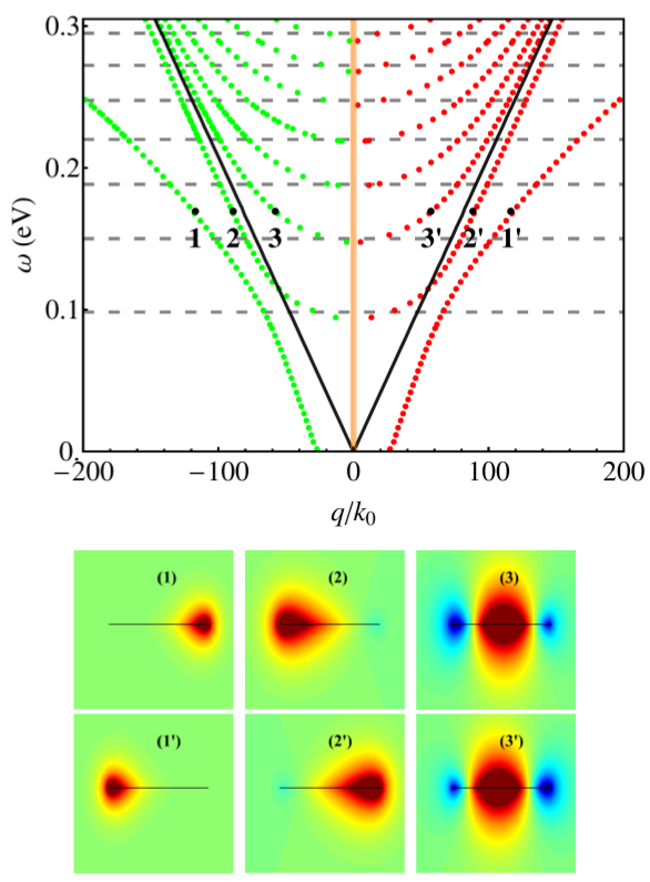
Figure 3: Guided modes in freestanding MDS ribbons. Ribbon width is assumed to be $w=$100\text{\,}\mathrm{n}\mathrm{m}$$. The grey dashed lines represents solutions of $k_{B}w+\phi_{R}=n\pi$, where $k_{B}$ is the bulk plasmon momentum in MDS and $\phi_{R}\approx-3\pi/4$Nikitin et al. (2014), which explains the cutoff for all the guided modes (except the edge mode). The black solid lines represent the bulk plasmon in a continuous sheet of MDS (same as Fig. 2). The color plots below represent the real part of the electric field along the ribbon at the indicated $q$.

This special coupling between the edge mode direction and the ribbon edge can be utilized to produce explicit nonreciproal devices. For instance, we can break the spatial symmetry between left and right by introducing another medium on one side of the ribbon. In the most extreme case, a perfect conductor can be used to short the edge mode on one sideSounas and Caloz (2011).

Valley induced giant polarization rotation– Polarization rotation is usually discussed in the context of magneto-optical materials (also called Faraday effect), where the plane of polarization of the incident wave is rotated upon passage through such a materialFaraday (1846). Cyclotron resonances in various two dimensional electron gasesSuzuki et al. (2003) were employed to produce this effect, with graphene being the most promising candidateCrassee et al. (2011). Optically induced valley polarization in a MDS presents a promising route to achieve a similar effect without the application of a static magnetic field, which can be cumbersome in the context of on-chip photonic components miniaturization.

We first consider polarization rotation in a continuous sheet of MDS. The polarization rotation angle is given byFerreira et al. (2011): $\theta_{F}\approx\Re\{\sigma_{xy}\}/2c\epsilon_{0}$ and the transmission by $T(\omega)\approx 1-\Re\{\sigma_{xx}\}/c\epsilon_{0}$. It should be noted that as opposed to optical activityZhang et al. (2012) which is reciprocal, the polarization rotation in our case is analogous to Faraday rotation which is a purely nonreciprocal effectPotton (2004). These equations suggest that the polarization rotation values in the continuous 2D sheet is only dependent on the $\sigma_{xy}$ which can be tuned by adjusting the intensity and polarization of the pump. Even with a pump intensity of the order of ${10^{8}}$V/m, rotation angle of only about ${0.1}$ degrees is obtained.

However, it is possible to use localized plasmon resonancesSepúlveda et al. (2010); Hadad et al. (2014) of nanoribbonsTymchenko et al. (2013) to enhance the polarization rotation values. In Fig. 4, we present the simulation results for transmission and polarization rotation in nanoribbons. We obtain significant enhancement of polarization rotation by more than an order of magnitude upon using nanoribbons as opposed to a continuous 2D sheet. Moreover, at the frequency of the resonant enhancement, transmitted intensity is still about $10-20\%$. The spectral location of the resonance is strongly tunable as a function of the ribbon width. These frequencies correspond to the solutions of $k_{B}w+\phi_{R}=n\pi$, as described earlier but with the constraint that $n$ is an even integerNikitin et al. (2014). Odd $n$ solutions are non-dipolar modes, hence do not couple with normally incident plane waves. The largest polarization rotation occurs for smaller ribbon sizes. This is because smaller ribbons, correspond to larger in-plane wavevectors, thus providing a higher field confinement. The polarization rotation we obtained with nanoribbons was found to even surpass Faraday rotation angles in monolayer graphene under a magnetic field of $7\text{\,}\mathrm{T}$Crassee et al. (2011).

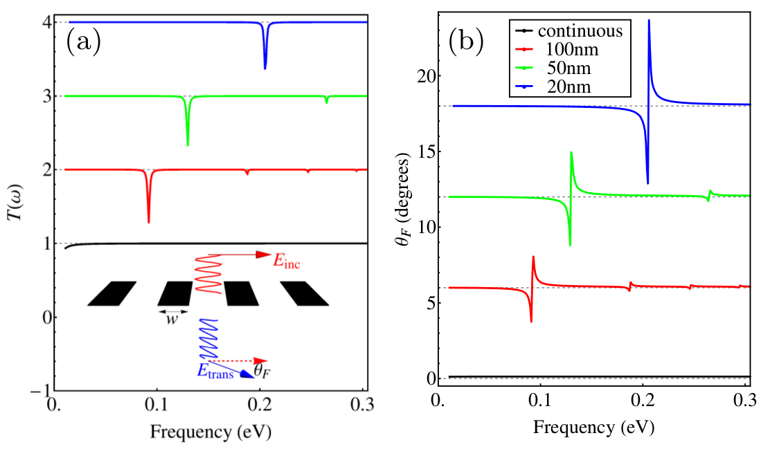
Figure 4: Transmission and polarization rotation in freestanding MDS ribbons: (a) Transmission (vertical offset is one unit). Inset: Schematic of the configuration. Note that in general the transmitted wave is expected to be elliptically polarized as opposed to linear as shown here. (b) polarization rotation spectrum for different ribbon sizes $w$ (vertical offset is 6 degrees). For ribbon arrays, a filling factor of 50% has been assumed.

Conclusion and summary— In summary, we have shown how polarization selective pumping in a generic gapped Dirac material can impart chirality to bulk and edge plasmons without the need for an external magnetic field. Experimentally testable predictions in the context of near field imaging, giant valley induced polarization rotation as well as nonreciprocal waveguiding were presented. Our theoretical approach can be applied to a general class of two dimensional materials with broken inversion symmetry. A rich array of nonreciprocal phenomenon can be potentially explored, from the point of view of applications to isolators, circulators, etc. Finally, since unlike a magnetic field, the field profile of the optical pump can be easily manipulated on the subwavelength scale by the use of nanostructuresMaier (2007), our work might pave the way for chip scale nonreciprocal photonics and optically tunable metasurfacesFallahi and Perruisseau-Carrier (2012); Kildishev et al. (2013).

During the preparation of our manuscript, we became aware of a related preprintSong and Rudner (2015).

Acknowledgement. A.K. and N.X.F. acknowledge the financial support by the NSF (grant CMMI-1120724) and AFOSR MURI (Award No. FA9550-12-1-0488). K.H.F. acknowledges financial support from Hong Kong RGC grant 15300315. T.L. acknowledges support from the MRSEC Program of the National Science Foundation under Award Number DMR-1420013.

I Von Neumann equation for density matrix

Evolution of electron subsystem in massive Dirac system (MDS) in external electromagnetic field $\mathbf{E}$ can be described using the von Neumann equation for electron statistical operator

$$i\hbar\frac{\partial\widehat{\rho}}{\partial t}=[\mathcal{H}+V,\widehat{\rho}\,]$$ (S1)

where $\mathcal{H}$ is the single-electron Hamiltonian of MDS, $\widehat{V}=-e\mathbf{E}\cdot\mathbf{r}$ is the interaction term, and $e=-1.6\times 10^{-19}$ is the electron charge. In the basis of eigenfunctions of $\mathcal{H}$ Eq. (S1) has the form

$$i\hbar\frac{\partial\rho_{\mathbf{k}j,\mathbf{k}^{\prime}j^{\prime}}}{\partial t}=[\mathcal{H},\widehat{\rho}\,]_{\mathbf{k}j,\mathbf{k}^{\prime}j^{\prime}}+[V,\widehat{\rho}\,]_{\mathbf{k}j,\mathbf{k}^{\prime}j^{\prime}},$$ (S2)

where

$$A_{\mathbf{k}j,\mathbf{k}^{\prime}j^{\prime}}=\int_{S}\Psi^{*}_{\mathbf{k}j}(\mathbf{r})\widehat{A}\Psi_{\mathbf{k}^{\prime}j^{\prime}}(\mathbf{r})d^{2}\mathbf{r},$$ (S3)

$\widehat{A}=\widehat{\rho},\mathcal{H},V$, $\mathbf{k}$ is two-dimensional electron wavevector, $j$ is an index designating quantum number of electrons in MDS. Integration is taken over the surface area $S$ of MDS. Functions $\Psi_{\mathbf{k}j}(\mathbf{r})$ are solutions of the equation

$$\mathcal{H}\Psi_{\mathbf{k}j}(\mathbf{r})=\mathcal{E}_{\mathbf{k}j}\Psi_{\mathbf{k}j}(\mathbf{r})$$ (S4)

and can be written in the Bloch form

$$\Psi_{\mathbf{k}j}(\mathbf{r})=\frac{1}{\sqrt{N}}\,e^{i\mathbf{k}\cdot\mathbf{r}}\,u_{\mathbf{k}j}(\mathbf{r}),$$ (S5)

where $N$ is the number of unit cells in MDS, and $u_{\mathbf{k}j}(\mathbf{r})=u_{\mathbf{k}j}(\mathbf{r}+\mathbf{R}_{n})$ is Bloch amplitude, $\mathbf{R}_{n}$ is the vector of MDS lattice.

First term on right-hand side of Eq. (S2) can be written as

$$[\mathcal{H},\widehat{\rho}\,]_{\mathbf{k}j,\mathbf{k}^{\prime}j^{\prime}} =\rho_{\mathbf{k}j,\mathbf{k}^{\prime}j^{\prime}}\left(\mathcal{E}_{\mathbf{k}j}-\mathcal{E}_{\mathbf{k}^{\prime}j^{\prime}}\right),$$ (S6)

while second term takes form

$$[V,\widehat{\rho}\,]_{\mathbf{k}j,\mathbf{k}^{\prime}j^{\prime}}=\sum_{\mathbf{k}^{\prime\prime}j^{\prime\prime}}\left(V_{\mathbf{k}j,\mathbf{k}^{\prime\prime}j^{\prime\prime}}\rho_{\mathbf{k}^{\prime\prime}j^{\prime\prime},\mathbf{k}^{\prime}j^{\prime}}-\rho_{\mathbf{k}j,\mathbf{k}^{\prime\prime}j^{\prime\prime}}V_{\mathbf{k}^{\prime\prime}j^{\prime\prime},\mathbf{k}^{\prime}j^{\prime}}\right).$$ (S7)

Let us consider first term on the left hand side of Eq. (S7),

$$\sum_{\mathbf{k}^{\prime\prime}j^{\prime\prime}}V_{\mathbf{k}j,\mathbf{k}^{\prime\prime}j^{\prime\prime}}\rho_{\mathbf{k}^{\prime\prime}j^{\prime\prime},\mathbf{k}^{\prime}j^{\prime}}=-e\mathbf{E}\cdot\sum\limits_{\mathbf{k}^{\prime\prime}j^{\prime\prime}}\rho_{\mathbf{k}^{\prime\prime}j^{\prime\prime},\mathbf{k}^{\prime}j^{\prime}}\int\limits_{S}\Psi_{\mathbf{k}j}^{*}(\mathbf{r})\mathbf{r}\,\Psi_{\mathbf{k}^{\prime\prime}j^{\prime\prime}}(\mathbf{r})d^{2}\mathbf{r}$$

$$=\frac{ie}{\sqrt{N}}\mathbf{E}\cdot\,\sum_{\mathbf{k}^{\prime\prime}j^{\prime\prime}}\rho_{\mathbf{k}^{\prime\prime}j^{\prime\prime},\mathbf{k}^{\prime}j^{\prime}}\int\limits_{S}\left[-\frac{\partial u_{\mathbf{k}j}^{*}(\mathbf{r})e^{-i\mathbf{k}\cdot\mathbf{r}}}{\partial\mathbf{k}}\,\Psi_{\mathbf{k}^{\prime\prime}j^{\prime\prime}}(\mathbf{r})+\frac{\partial u_{\mathbf{k}j}^{*}(\mathbf{r})}{\partial\mathbf{k}}e^{-i\mathbf{k}\cdot\mathbf{r}}\Psi_{\mathbf{k}^{\prime\prime}j^{\prime\prime}}(\mathbf{r})\right]d^{2}\mathbf{r}$$ (S8)

As electron wavefunctions are normalized,

$$\int\limits_{S}\Psi_{\mathbf{k}j}^{*}(\mathbf{r})\Psi_{\mathbf{k}^{\prime}j^{\prime}}(\mathbf{r})d^{2}\mathbf{r}=\delta_{\mathbf{k}\mathbf{k}^{\prime}}\delta_{jj^{\prime}},$$ (S9)

the first term in square brackets in Eq. (S8) takes form

$$\frac{1}{\sqrt{N}}\sum_{\mathbf{k}^{\prime\prime}j^{\prime\prime}}\rho_{\mathbf{k}^{\prime\prime}j^{\prime\prime},\mathbf{k}^{\prime}j^{\prime}}\int\limits_{S}\frac{\partial u_{\mathbf{k}j}^{*}(\mathbf{r})e^{-i\mathbf{k}\cdot\mathbf{r}}}{\partial\mathbf{k}}\,\Psi_{\mathbf{k}^{\prime\prime}j^{\prime\prime}}(\mathbf{r})d^{2}\mathbf{r}=\frac{\partial}{\partial\mathbf{k}}\sum_{\mathbf{k}^{\prime\prime}j^{\prime\prime}}\rho_{\mathbf{k}^{\prime\prime}j^{\prime\prime},\mathbf{k}^{\prime}j^{\prime}}\int\limits_{S}\Psi_{\mathbf{k}j}^{*}(\mathbf{r})\Psi_{\mathbf{k}^{\prime\prime}j^{\prime\prime}}(\mathbf{r})d^{2}\mathbf{r}=\frac{\partial\rho_{\mathbf{k}j,\mathbf{k}^{\prime}j^{\prime}}}{\partial\mathbf{k}}.$$ (S10)

In order to simplify the second term in the square brackets we split integral over the surface area $S$ as sum of integrals over unit cells $\Omega_{n}$:

$$\frac{1}{N}\int\limits_{S}\frac{\partial u_{\mathbf{k}j}^{*}(\mathbf{r})}{\partial\mathbf{k}}u_{\mathbf{k}^{\prime\prime}j^{\prime\prime}}(\mathbf{r})e^{i(\mathbf{k}^{\prime\prime}-\mathbf{k})\cdot\mathbf{r}}d^{2}\mathbf{r}=\frac{1}{N}\sum_{n=1}^{N}\int\limits_{\Omega_{n}}\frac{\partial u_{\mathbf{k}j}^{*}(\mathbf{r})}{\partial\mathbf{k}}u_{\mathbf{k}^{\prime\prime}j^{\prime\prime}}(\mathbf{r})e^{i(\mathbf{k}^{\prime\prime}-\mathbf{k})\cdot\mathbf{r}}d^{2}\mathbf{r}$$

$$=\frac{1}{N}\sum_{n=1}^{N}\int\limits_{\Omega_{1}}\frac{\partial u_{\mathbf{k}j}^{*}(\mathbf{r}+\mathbf{R}_{n})}{\partial\mathbf{k}}u_{\mathbf{k}^{\prime\prime}j^{\prime\prime}}(\mathbf{r}+\mathbf{R}_{n})e^{i(\mathbf{k}^{\prime\prime}-\mathbf{k})\cdot(\mathbf{r}+\mathbf{R}_{n})}d^{2}\mathbf{r}$$

$$=\frac{1}{N}\sum_{n=1}^{N}e^{i(\mathbf{k}^{\prime\prime}-\mathbf{k})\cdot\mathbf{R}_{n}}\int\limits_{\Omega_{1}}\frac{\partial u_{\mathbf{k}j}^{*}(\mathbf{r})}{\partial\mathbf{k}}u_{\mathbf{k}^{\prime\prime}j^{\prime\prime}}(\mathbf{r})e^{i(\mathbf{k}^{\prime\prime}-\mathbf{k})\cdot\mathbf{r}}d^{2}\mathbf{r}$$

$$=\delta_{\mathbf{k}\mathbf{k}^{\prime\prime}}\int_{\Omega_{1}}\frac{\partial u_{\mathbf{k}j}^{*}(\mathbf{r})}{\partial\mathbf{k}}u_{\mathbf{k}j^{\prime\prime}}(\mathbf{r})d^{2}\mathbf{r}=-\delta_{\mathbf{k}\mathbf{k}^{\prime\prime}}\int_{\Omega_{1}}u_{\mathbf{k}j}^{*}(\mathbf{r})\frac{\partial u_{\mathbf{k}j^{\prime\prime}}(\mathbf{r})}{\partial\mathbf{k}}d^{2}\mathbf{r}.$$ (S11)

In order to obtain last expression we integrated by parts and took into account periodicity of Bloch amplitudes at the unit cell boundaries.

Plugging Eqs. (S10), (S11) back into Eq. (S8) we obtain

$$(V\widehat{\rho})_{\mathbf{k}j,\mathbf{k}^{\prime}j^{\prime}}=-i\,e\,\mathbf{E}\cdot\frac{\partial\rho_{\mathbf{k}j,\mathbf{k}^{\prime}j^{\prime}}}{\partial\mathbf{k}}-e\,\mathbf{E}\cdot\sum_{j^{\prime\prime}}\mathbf{R}_{jj^{\prime\prime}}(\mathbf{k})\rho_{\mathbf{k}j^{\prime\prime},\mathbf{k}^{\prime}j^{\prime}},$$ (S12)

where

$$\mathbf{R}_{jj^{\prime\prime}}(\mathbf{k})=\frac{i}{2}\int_{\Omega_{1}}\left(u_{\mathbf{k}j}^{*}(\mathbf{r})\frac{\partial u_{\mathbf{k}j^{\prime\prime}}(\mathbf{r})}{\partial\mathbf{k}}-\frac{\partial u_{\mathbf{k}j}^{*}(\mathbf{r})}{\partial\mathbf{k}}u_{\mathbf{k}j^{\prime\prime}}(\mathbf{r})\right)d^{2}\mathbf{r}.$$ (S13)

Repeating the steps above we also obtain

$$(\widehat{\rho}\,V)_{\mathbf{k}j,\mathbf{k}^{\prime}j^{\prime}} =ie\,\mathbf{E}\cdot\frac{\partial\rho_{\mathbf{k}j,\mathbf{k}^{\prime}j^{\prime}}}{\partial\mathbf{k}^{\prime}}-e\,\mathbf{E}\cdot\sum_{j^{\prime\prime}}\rho_{\mathbf{k}j,\mathbf{k}^{\prime}j^{\prime\prime}}\mathbf{R}_{j^{\prime\prime}j^{\prime}}(\mathbf{k}^{\prime}),$$ (S14)

and

$$[V,\widehat{\rho}\,]_{\mathbf{k}j,\mathbf{k}^{\prime}j^{\prime}} =-i\,e\,\mathbf{E}\cdot\left(\frac{\partial\rho_{\mathbf{k}j,\mathbf{k}^{\prime}j^{\prime}}}{\partial\mathbf{k}}+\frac{\partial\rho_{\mathbf{k}j,\mathbf{k}^{\prime}j^{\prime}}}{\partial\mathbf{k}^{\prime}}\right)-e\,\mathbf{E}\cdot\sum_{j^{\prime\prime}}\left(\mathbf{R}_{jj^{\prime\prime}}(\mathbf{k})\rho_{\mathbf{k}j^{\prime\prime},\mathbf{k}^{\prime}j^{\prime}}-\rho_{\mathbf{k}j,\mathbf{k}^{\prime}j^{\prime\prime}}\mathbf{R}_{j^{\prime\prime}j^{\prime}}(\mathbf{k}^{\prime})\right).$$ (S15)

Thus, the equation of motion for the electron density matrix takes form

$$i\hbar\frac{\partial\rho_{\mathbf{k}j,\mathbf{k}^{\prime}j^{\prime}}}{\partial t}=\rho_{\mathbf{k}j,\mathbf{k}^{\prime}j^{\prime}}\left(\mathcal{E}_{\mathbf{k}j}-\mathcal{E}_{\mathbf{k}^{\prime}j^{\prime}}\right)-i\,e\,\mathbf{E}\cdot\left(\frac{\partial\rho_{\mathbf{k}j,\mathbf{k}^{\prime}j^{\prime}}}{\partial\mathbf{k}}+\frac{\partial\rho_{\mathbf{k}j,\mathbf{k}^{\prime}j^{\prime}}}{\partial\mathbf{k}^{\prime}}\right)$$

$$-e\,\mathbf{E}\cdot\sum_{j^{\prime\prime}}\left(\mathbf{R}_{jj^{\prime\prime}}(\mathbf{k})\rho_{\mathbf{k}j^{\prime\prime},\mathbf{k}^{\prime}j^{\prime}}-\rho_{\mathbf{k}j,\mathbf{k}^{\prime}j^{\prime\prime}}\mathbf{R}_{j^{\prime\prime}j^{\prime}}(\mathbf{k}^{\prime})\right).$$ (S16)

Eq. (S16) accounts both for the intraband motions and direct and indirect interband transitions. However, contribution of electrons indirect interband transitions to the optical response is negligible and thus can be omitted. Then, in the limit $\mathbf{k}^{\prime}\to\mathbf{k}$, we obtain

$$\frac{\partial\rho_{jj^{\prime}}(t,\mathbf{k})}{\partial t}+\frac{e}{\hbar}\mathbf{E}\cdot\frac{\partial\rho_{jj^{\prime}}(t,\mathbf{k})}{\partial\mathbf{k}} =-\frac{i}{\hbar}\rho_{jj^{\prime}}(t,\mathbf{k})[\mathcal{E}_{\mathbf{k}j}-\mathcal{E}_{\mathbf{k}^{\prime}j^{\prime}}]$$

$$+\frac{i\,e}{\hbar}\,\mathbf{E}\cdot\sum_{j^{\prime\prime}}\left[\mathbf{R}_{jj^{\prime\prime}}(\mathbf{k})\rho_{j^{\prime\prime}j^{\prime}}(t,\mathbf{k})-\rho_{jj^{\prime\prime}}(t,\mathbf{k})\mathbf{R}_{j^{\prime\prime}j^{\prime}}(\mathbf{k})\right],$$ (S17)

where $\rho_{jj^{\prime}}(t,\mathbf{k})=\rho_{\mathbf{k}j,\mathbf{k}^{\prime}j^{\prime}}(t)$, where $\nu,\mu=c,v$ denote electron and hole bands.

II Incorporating relaxation into equations of motion for density matrix

Electromagnetic radiation can not also couple electrons in different valleys in $\mathbf{k}$-space, and thus it is convenient to write equations separately for each of the valleys. We account for different valleys by introducing valley quantum number $\tau=\pm 1$ (or $K,K^{\prime}$). For convenience, we designate density matrix elements as $\rho_{jj^{\prime}}(t,\mathbf{k})=\rho^{\tau}_{\nu\mu}(t,\mathbf{k})$.

We introduce relaxation phenomenologically using relaxation time approximation. Then the equation for the density matrix of electrons in conduction band in $K$ valley takes form

$$\frac{\partial\rho_{cc}^{K}(t,\mathbf{k})}{\partial t}+\frac{e}{\hbar}\mathbf{E}\cdot\frac{\partial\rho_{cc}^{K}(t,\mathbf{k})}{\partial\mathbf{k}}= -\frac{\rho_{cc}^{K}(t,\mathbf{k})-\rho_{cc}^{\mathrm{eq},K}(\mathbf{k})}{\tau_{0}}+\frac{\rho_{cc}^{K^{\prime}}(t,\mathbf{k})-\rho_{cc}^{K}(t,\mathbf{k})}{\tau_{1}}$$

$$+\frac{i\,e}{\hbar}\,\mathbf{E}\cdot\left[\mathbf{R}_{cv}^{K}(\mathbf{k})\rho_{vc}^{K}(t,\mathbf{k})-\rho_{cv}^{K}(t,\mathbf{k})\mathbf{R}_{vc}^{K}(\mathbf{k})\right],$$ (S18)

where $\rho_{cc}^{\mathrm{eq},K}(\mathbf{k})$ is equillibrium Fermi-Dirac distribution, $\tau_{0}$ is the population relaxation time. We also took into account that electron-phonon interactions can couple electrons in different valleys by introducing inter-valley scattering time $\tau_{1}$. The rest of equations for diagonal matrix elements can be written as

$$\frac{\partial\rho_{cc}^{K^{\prime}}}{\partial t}+\frac{e}{\hbar}\mathbf{E}\cdot\frac{\partial\rho_{cc}^{K^{\prime}}}{\partial\mathbf{k}} =-\frac{\rho_{cc}^{K^{\prime}}-\rho_{cc}^{\mathrm{eq},K^{\prime}}}{\tau_{0}}+\frac{\rho_{cc}^{K}-\rho_{cc}^{K^{\prime}}}{\tau_{1}}+\frac{i\,e}{\hbar}\,\mathbf{E}\cdot\left[\mathbf{R}_{cv}^{K^{\prime}}\rho_{vc}^{K^{\prime}}-\rho_{cv}^{K^{\prime}}\mathbf{R}_{vc}^{K^{\prime}}\right],$$ (S19)

$$\frac{\partial\rho_{vv}^{K}}{\partial t}+\frac{e}{\hbar}\mathbf{E}\cdot\frac{\partial\rho_{vv}^{K}}{\partial\mathbf{k}} =-\frac{\rho_{vv}^{K}-\rho_{vv}^{\mathrm{eq},K}}{\tau_{0}}+\frac{\rho_{vv}^{K^{\prime}}-\rho_{vv}^{K}}{\tau_{1}}-\frac{i\,e}{\hbar}\,\mathbf{E}\cdot\left[\mathbf{R}_{cv}^{K}\rho_{vc}^{K}-\rho_{cv}^{K}\mathbf{R}_{vc}^{K}\right],$$ (S20)

$$\frac{\partial\rho_{vv}^{K^{\prime}}}{\partial t}+\frac{e}{\hbar}\mathbf{E}\cdot\frac{\partial\rho_{vv}^{K^{\prime}}}{\partial\mathbf{k}} =-\frac{\rho_{vv}^{K^{\prime}}-\rho_{vv}^{\mathrm{eq},{K^{\prime}}}}{\tau_{0}}+\frac{\rho_{vv}^{K}-\rho_{vv}^{K^{\prime}}}{\tau_{1}}-\frac{i\,e}{\hbar}\,\mathbf{E}\cdot\left[\mathbf{R}_{cv}^{K^{\prime}}\rho_{vc}^{K^{\prime}}-\rho_{cv}^{K^{\prime}}\mathbf{R}_{vc}^{K^{\prime}}\right].$$ (S21)

The non-diagonal matrix elements evolve as

$$\frac{\partial\rho_{cv}^{K}}{\partial t}+\frac{e}{\hbar}\mathbf{E}\cdot\frac{\partial\rho_{cv}^{K}}{\partial\mathbf{k}} =-\left(i\omega_{cv}^{K}+\frac{1}{\tau_{d}}\right)\rho_{cv}^{K}+\frac{2i\,e}{\hbar}\,\mathbf{E}\cdot\mathbf{R}_{cc}^{K}\rho_{cv}^{K}-\frac{i\,e}{\hbar}\,\mathbf{E}\cdot\mathbf{R}_{cv}^{K}\rho_{\mathrm{in}}^{K},$$ (S22)

where $\rho_{\mathrm{in}}^{K}=\rho_{cc}^{K}-\rho_{vv}^{K}$, $\omega_{cv}^{K}=\left(\mathcal{E}_{c}^{K}-\mathcal{E}_{v}^{K}\right)/\hbar$, and $\tau_{d}$ is electron dephasing time.

III Eigenenergies and eigenfunctions

In order to calculate dipole matrix elements we need to know Bloch amplitudes $u_{\mathbf{k}j}$. We use MDS Hamiltonian

$${\cal H}=\frac{\Delta}{2}\sigma_{z}+t_{0}a_{0}\textbf{k}\cdot\bm{\sigma}_{\tau},$$

where $\bm{\sigma}_{\tau}=(\tau\sigma_{x},\sigma_{y})$. After diagonalizing the Hamiltonian, we obtain eigenenergies

$$\mathcal{E}^{\tau}_{\mathbf{k}\nu}=\frac{\nu}{2}\sqrt{\beta^{\tau}_{\mathbf{k}}},$$ (S23)

and eigenfunctions

$$u^{\tau}_{\mathbf{k}c}=\frac{1}{\sqrt{S_{\Omega}}\,|\Phi^{\tau}_{\mathbf{k}}|}\left(\begin{array}[]{c}1\\ W^{\tau}_{\mathbf{k}}\end{array}\right),\quad u^{\tau}_{\mathbf{k}v}=\frac{1}{\sqrt{S_{\Omega}}\,|\Phi^{\tau}_{\mathbf{k}}|}\left(\begin{array}[]{c}-W^{\tau*}_{\mathbf{k}}\\ 1\end{array}\right),$$ (S24)

where

$$W^{\tau}_{\mathbf{k}}=\frac{2t_{0}a_{0}\left(\tau k_{x}+ik_{y}\right)}{\Delta+\sqrt{\beta^{\tau}_{\mathbf{k}}}},\quad|\Phi^{\tau}_{\mathbf{k}}|^{2}=1+|W^{\tau}_{\mathbf{k}}|^{2},$$ (S25)

$$\beta^{\tau}_{\mathbf{k}}=4a_{0}^{2}t_{0}^{2}k^{2}+\Delta^{2},$$ (S26)

$\nu=\pm 1$ denotes conduction and valence band respectively, and $S_{\Omega}$ is an area of unit cell.

IV Dipole matrix elements $\mathbf{R}_{jj^{\prime}}$

$$\mathbf{R}_{cc}^{\tau}(\mathbf{k})=\frac{i}{2}\int_{\Omega_{1}}\left(u_{\mathbf{k}c}^{\tau*}\frac{\partial u^{\tau}_{\mathbf{k}c}}{\partial\mathbf{k}}-\frac{\partial u_{\mathbf{k}c}^{\tau*}}{\partial\mathbf{k}}u_{\mathbf{k}c}^{\tau}\right)d^{2}\mathbf{r}=\frac{i}{2|\Phi^{\tau}_{\mathbf{k}}|^{2}}\left(W_{\mathbf{k}}^{\tau*}\frac{\partial W_{\mathbf{k}}^{\tau}}{\partial\mathbf{k}}-W_{\mathbf{k}}^{\tau}\frac{\partial W_{\mathbf{k}}^{\tau*}}{\partial\mathbf{k}}\right)$$

$$=-\frac{\tau\Omega_{\mathbf{k}\tau}^{2}}{|\Phi^{\tau}_{\mathbf{k}}|^{2}}\left(\begin{array}[]{c}-k_{y}\\ k_{x}\end{array}\right),$$ (S29)

$$\mathbf{R}_{vv}^{\tau}(\mathbf{k})=\frac{i}{2}\int_{\Omega_{1}}\left(u_{\mathbf{k}v}^{\tau*}\frac{\partial u^{\tau}_{\mathbf{k}v}}{\partial\mathbf{k}}-\frac{\partial u_{\mathbf{k}v}^{\tau*}}{\partial\mathbf{k}}u_{\mathbf{k}v}^{\tau}\right)d^{2}\mathbf{r}=-\frac{i}{2|\Phi^{\tau}_{\mathbf{k}}|^{2}}\left(W_{\mathbf{k}}^{\tau*}\frac{\partial W_{\mathbf{k}}^{\tau}}{\partial\mathbf{k}}-W_{\mathbf{k}}^{\tau}\frac{\partial W_{\mathbf{k}}^{\tau*}}{\partial\mathbf{k}}\right)$$

$$=\frac{\tau\Omega_{\mathbf{k}\tau}^{2}}{|\Phi^{\tau}_{\mathbf{k}}|^{2}}\left(\begin{array}[]{c}-k_{y}\\ k_{x}\end{array}\right),$$ (S32)

$$\mathbf{R}_{cv}^{\tau}(\mathbf{k})=\frac{i}{2}\int_{\Omega_{1}}\left(u_{\mathbf{k}c}^{\tau*}\frac{\partial u^{\tau}_{\mathbf{k}v}}{\partial\mathbf{k}}-\frac{\partial u_{\mathbf{k}c}^{\tau*}}{\partial\mathbf{k}}u_{\mathbf{k}v}^{\tau}\right)d^{2}\mathbf{r}=-\frac{i}{|\Phi^{\tau}_{\mathbf{k}}|^{2}}\frac{\partial W_{\mathbf{k}}^{\tau*}}{\partial\mathbf{k}}$$

$$=\frac{a_{0}t}{\sqrt{\beta^{\tau}_{\mathbf{k}}}\alpha^{\tau}_{\mathbf{k}}}\left(\begin{array}[]{c}4a_{0}^{2}t^{2}k_{x}k_{y}-i\tau\left(\alpha^{\tau}_{\mathbf{k}}-4a_{0}^{2}t^{2}k_{x}^{2}\right)\\ -\alpha^{\tau}_{\mathbf{k}}+4a_{0}^{2}t^{2}k_{y}^{2}+4i\tau a_{0}^{2}t^{2}k_{x}k_{y}\end{array}\right),$$ (S35)

$$\Omega_{\mathbf{k}\tau}=\frac{2t_{0}a_{0}}{\Delta+\sqrt{\beta^{\tau}_{\mathbf{k}}}},$$ (S36)

$$\alpha^{\tau}_{\mathbf{k}}=\sqrt{\beta^{\tau}_{\mathbf{k}}}\left(\sqrt{\beta^{\tau}_{\mathbf{k}}}+\Delta\right).$$ (S37)

Dot product $\mathbf{E}_{0}\cdot\mathbf{R}_{cv}^{K,K^{\prime}}$ defines valley interaction with a field of a given polarization. Let us assume that $\mathbf{E}_{0}=|\mathbf{E}_{0}|(\mathbf{e}_{x}+i\mathbf{e}_{y})$. Then for $K$ valley ($\tau_{z}=1$)

$$\mathbf{E}_{0}\cdot\mathbf{R}_{cv}^{K}=|\mathbf{E}_{0}|\frac{a_{0}t\left(-2i\alpha^{K}_{\mathbf{k}}+4ia_{0}^{2}t^{2}(k_{x}^{2}+k_{y}^{2})\right)}{\sqrt{\beta^{K}_{\mathbf{k}}}\alpha^{K}_{\mathbf{k}}}$$ (S38)

In the case $k_{x}=k_{y}=0$

$$\mathbf{E}_{0}\cdot\mathbf{R}_{cv}^{K}=-2i|\mathbf{E}_{0}|\frac{a_{0}t}{\sqrt{\beta^{K}_{\mathbf{k}}}}.$$ (S39)

Thus (+) polarized wave pumps K valley. Let us consider $K^{\prime}$ valley ($\tau_{z}=-1$) now:

$$\mathbf{E}_{0}\cdot\mathbf{R}_{cv}^{K^{\prime}}=|\mathbf{E}_{0}|\frac{4ia_{0}^{3}t^{3}(k_{y}^{2}-k_{x}^{2})}{\sqrt{\beta^{K}_{\mathbf{k}}}\alpha^{K}_{\mathbf{k}}}$$ (S40)

In the case $k_{x}=k_{y}=0$

$$\mathbf{E}_{0}\cdot\mathbf{R}_{cv}^{K^{\prime}}=0.$$ (S41)

Thus electrons in K’ valley do not interact with (+) polarized wave.

V MDS interaction with laser pump

Let us consider interaction of MDS with monochromatic electromagnetic wave

$$\mathbf{E}=\mathbf{E}_{0}e^{-i\omega t}+c.c..$$ (S42)

We assume that frequency of the wave $\omega$ is in the vicinity of the frequency of electron interband transitions. Eqs. (II)-(S22) are partial differential equations which have to be solved numerically in the general case. However, in the case of near-resonant wave interband electron transitions dominate intraband motion. Thus we can neglect terms containing partial derivatives over $\mathbf{k}$ on the right-hand side.

Under the influence of electromagnetic field non-diagonal matrix elements evolve as $\rho_{cv}=\tilde{\rho}_{cv}(t)e^{-i\omega t}$, where $\tilde{\rho}_{cv}(t)$ is a slow varying amplitude. We are interested in the steady-state solution. Using the rotation-wave approximation and setting partial derivative of $\tilde{\rho}_{cv}(t)$ to zero, we obtain

$$\tilde{\rho}_{cv}^{\tau} =\frac{e}{\hbar\left(\omega-\omega_{cv}^{\tau}+i/\tau_{d}\right)}\,\mathbf{E}_{0}\cdot\mathbf{R}_{cv}^{\tau}\rho_{\mathrm{in}}^{\tau}.$$ (S43)

Eqs. (II)-(S21) then take form

$$0 =-\frac{\rho_{cc}^{K}-\rho_{cc}^{\mathrm{eq},K}}{\tau_{0}}+\frac{\rho_{cc}^{K^{\prime}}-\rho_{cc}^{K}}{\tau_{1}}+\frac{i\,e}{\hbar}\,\left[\mathbf{E}_{0}\cdot\mathbf{R}_{cv}^{K}\tilde{\rho}_{cv}^{K*}-\mathbf{E}_{0}^{*}\cdot\mathbf{R}_{vc}^{K}\tilde{\rho}_{cv}^{K}\right],$$ (S44)

$$0 =-\frac{\rho_{cc}^{K^{\prime}}-\rho_{cc}^{\mathrm{eq},K^{\prime}}}{\tau_{0}}+\frac{\rho_{cc}^{K}-\rho_{cc}^{K^{\prime}}}{\tau_{1}}+\frac{i\,e}{\hbar}\,\left[\mathbf{E}_{0}\cdot\mathbf{R}_{cv}^{K^{\prime}}\tilde{\rho}_{cv}^{K^{\prime}*}-\mathbf{E}_{0}^{*}\cdot\mathbf{R}_{vc}^{K^{\prime}}\tilde{\rho}_{cv}^{K^{\prime}}\right],$$ (S45)

$$0 =-\frac{\rho_{vv}^{K}-\rho_{vv}^{\mathrm{eq},K}}{\tau_{0}}+\frac{\rho_{vv}^{K^{\prime}}-\rho_{vv}^{K}}{\tau_{1}}-\frac{i\,e}{\hbar}\,\left[\mathbf{E}_{0}\cdot\mathbf{R}_{cv}^{K}\tilde{\rho}_{cv}^{K*}-\mathbf{E}_{0}^{*}\cdot\mathbf{R}_{vc}^{K}\tilde{\rho}_{cv}^{K}\right],$$ (S46)

$$0 =-\frac{\rho_{vv}^{K^{\prime}}-\rho_{vv}^{\mathrm{eq},K^{\prime}}}{\tau_{0}}+\frac{\rho_{vv}^{K}-\rho_{vv}^{K^{\prime}}}{\tau_{1}}-\frac{i\,e}{\hbar}\,\left[\mathbf{E}_{0}\cdot\mathbf{R}_{cv}^{K^{\prime}}\tilde{\rho}_{cv}^{K^{\prime}*}-\mathbf{E}_{0}^{*}\cdot\mathbf{R}_{vc}^{K^{\prime}}\tilde{\rho}_{cv}^{K^{\prime}}\right].$$ (S47)

By substituting Eq. (S43) into equations (S44)-(S47), we obtain system of four linear equations for diagonal matrix elements in two valleys

$$\rho_{vv}^{K} =\beta_{K}\left(\rho_{vv}^{\mathrm{eq},K}+\gamma\rho_{vv}^{K^{\prime}}+\alpha_{K}\rho_{cc}^{K}\right),$$

$$\rho_{vv}^{K^{\prime}} =\beta_{K^{\prime}}\left(\rho_{vv}^{\mathrm{eq},K^{\prime}}+\gamma\rho_{vv}^{K}+\alpha_{K^{\prime}}\rho_{cc}^{K^{\prime}}\right),$$

$$\rho_{cc}^{K} =\beta_{K}\left(\rho_{cc}^{\mathrm{eq},K}+\gamma\rho_{cc}^{K^{\prime}}+\alpha_{K}\rho_{vv}^{K}\right),$$

$$\rho_{cc}^{K^{\prime}} =\beta_{K^{\prime}}\left(\rho_{cc}^{\mathrm{eq},K^{\prime}}+\gamma\rho_{cc}^{K}+\alpha_{K^{\prime}}\rho_{vv}^{K^{\prime}}\right)$$

where

$$\beta_{K}=\frac{1}{1+\alpha_{K}+\gamma},\qquad\gamma=\frac{\tau_{0}}{\tau_{1}},$$

$$\alpha_{K,K^{\prime}}=\frac{2e^{2}\tau_{0}\tau_{d}|\mathbf{E}_{0}\cdot\mathbf{R}_{cv}^{K,K^{\prime}}|^{2}}{\hbar^{2}\left(\tau_{d}^{2}(\omega-\omega_{cv}^{K,K^{\prime}})^{2}+1\right)}.$$

In the paper we assumed that $\tau_{d}=\tau_{0}$.

References

• Berry (1984) M. V. Berry, in Proceedings of the Royal Society of London A: Mathematical, Physical and Engineering Sciences, Vol. 392 (The Royal Society, 1984) pp. 45–57.
• Xiao et al. (2010) D. Xiao, M.-C. Chang,  and Q. Niu, Reviews of modern physics 82, 1959 (2010).
• Nagaosa et al. (2010) N. Nagaosa, J. Sinova, S. Onoda, A. MacDonald,  and N. Ong, Reviews of modern physics 82, 1539 (2010).
• Hasan and Kane (2010) M. Z. Hasan and C. L. Kane, Reviews of Modern Physics 82, 3045 (2010).
• Xiao et al. (2012) D. Xiao, G.-B. Liu, W. Feng, X. Xu,  and W. Yao, Physical Review Letters 108, 196802 (2012).
• Mak et al. (2014) K. F. Mak, K. L. McGill, J. Park,  and P. L. McEuen, Science 344, 1489 (2014).
• Gorbachev et al. (2014) R. Gorbachev, J. Song, G. Yu, A. Kretinin, F. Withers, Y. Cao, A. Mishchenko, I. Grigorieva, K. Novoselov, L. Levitov, et al., Science 346, 448 (2014).
• Sui et al. (2015) M. Sui, G. Chen, L. Ma, W. Shan, D. Tian, K. Watanabe, T. Taniguchi, X. Jin, W. Yao, D. Xiao, et al., arXiv preprint arXiv:1501.04685  (2015).
• Grigorenko et al. (2012) A. N. Grigorenko, M. Polini,  and K. S. Novoselov, Nat. Photonics 6, 749 (2012).
• Koppens et al. (2011) F. H. L. Koppens, D. E. Chang,  and F. J. García de Abajo, Nano Lett. 11, 3370 (2011).
• Jablan et al. (2009) M. Jablan, H. Buljan,  and M. Soljačić, Phys. Rev. B 80, 245435 (2009).
• Low and Avouris (2014) T. Low and P. Avouris, ACS Nano 8, 1086 (2014), pMID: 24484181.
• Giuliani and Vignale (2005) G. Giuliani and G. Vignale, Quantum Theory of the Electron Liquid (Cambridge University Press, 2005).
• Slepyan et al. (2004) G. Y. Slepyan, A. A. Khrutchinski, A. M. Nemilentsau, S. A. Maksimenko,  and J. Herrmann, International Journal of Nanoscience 03, 343 (2004).
• Nemilentsau et al. (2006) A. Nemilentsau, G. Slepyan, A. Khrutchinskii,  and S. Maksimenko, Carbon 44, 2246 (2006).
• Neto et al. (2009) A. C. Neto, F. Guinea, N. Peres, K. S. Novoselov,  and A. K. Geim, Reviews of modern physics 81, 109 (2009).
• Li and Carbotte (2012) Z. Li and J. P. Carbotte, Phys. Rev. B 86, 205425 (2012).
• Chiu and Quinn (1974) K. W. Chiu and J. J. Quinn, Phys. Rev. B 9, 4724 (1974).
• Hanson (2008) G. Hanson, Antennas and Propagation, IEEE Transactions on 56, 747 (2008).
• Yudin et al. (2015) D. Yudin, O. Eriksson,  and M. I. Katsnelson, Phys. Rev. B 91, 075419 (2015).
• Fetter (1985) A. L. Fetter, Phys. Rev. B 32, 7676 (1985).
• Camley (1987) R. Camley, Surface Science Reports 7, 103 (1987).
• Wang et al. (2012) W. Wang, J. M. Kinaret,  and S. P. Apell, Phys. Rev. B 85, 235444 (2012).
• le Feber et al. (2015) B. le Feber, N. Rotenberg,  and L. Kuipers, Nat Commun 6,  (2015).
• Raether (1988) H. Raether, Surface Plasmons on Smooth and Rough Surfaces and on Gratings (Springer, 1988).
• Fei et al. (2011) Z. Fei, G. O. Andreev, W. Bao, L. M. Zhang, A. S. McLeod, C. Wang, M. K. Stewart, Z. Zhao, G. Dominguez, M. Thiemens, M. M. Fogler, M. J. Tauber, A. H. Castro-Neto, C. N. Lau, F. Keilmann,  and D. N. Basov, Nano Letters 11, 4701 (2011), pMID: 21972938.
• Fei et al. (2012) Z. Fei, A. S. Rodin, G. O. Andreev, W. Bao, A. S. McLeod, M. Wagner, L. M. Zhang, Z. Zhao, M. Thiemens, G. Dominguez, M. M. Fogler, A. H. C. Neto, C. N. Lau, F. Keilmann,  and D. N. Basov, Nature 487, 82 (2012).
• Chen et al. (2012) J. Chen, M. Badioli, P. Alonso-González, S. Thongrattanasiri, F. Huth, J. Osmond, M. Spasenović, A. Centeno, A. Pesquera, P. Godignon, A. Z. Elorza, N. Camara, F. J. G. de Abajo, R. Hillenbrand,  and F. H. L. Koppens, Nature 487, 77 (2012).
• Sounas and Caloz (2011) D. L. Sounas and C. Caloz, Applied Physics Letters 99, 231902 (2011).
• Fang and Sun (2015) Y. Fang and M. Sun, Light Sci Appl 4, e294 (2015).
• Nikitin et al. (2011) A. Y. Nikitin, F. Guinea, F. J. García-Vidal,  and L. Martín-Moreno, Phys. Rev. B 84, 161407 (2011).
• Christensen et al. (2012) J. Christensen, A. Manjavacas, S. Thongrattanasiri, F. H. L. Koppens,  and F. J. García de Abajo, ACS Nano 6, 431 (2012), pMID: 22147667.
• Manjavacas and García de Abajo (2009) A. Manjavacas and F. J. García de Abajo, Nano Letters 9, 1285 (2009), pMID: 18672946.
• Nikitin et al. (2014) A. Y. Nikitin, T. Low,  and L. Martin-Moreno, Phys. Rev. B 90, 041407 (2014).
• Faraday (1846) M. Faraday, Phil. Trans. R. Soc. 136, 104 (1846).
• Suzuki et al. (2003) M. Suzuki, K. ichi Fujii, T. Ohyama, H. Kobori,  and N. Kotera, Journal of the Physical Society of Japan 72, 3276 (2003).
• Crassee et al. (2011) I. Crassee, J. Levallois, A. L. Walter, M. Ostler, A. Bostwick, E. Rotenberg, T. Seyller, D. van der Marel,  and A. B. Kuzmenko, Nat. Phys. 7, 48 (2011).
• Ferreira et al. (2011) A. Ferreira, J. Viana-Gomes, Y. V. Bludov, V. Pereira, N. M. R. Peres,  and A. H. Castro Neto, Phys. Rev. B 84, 235410 (2011).
• Zhang et al. (2012) S. Zhang, J. Zhou, Y.-S. Park, J. Rho, R. Singh, S. Nam, A. K. Azad, H.-T. Chen, X. Yin, A. J. Taylor,  and X. Zhang, Nat Commun 3, 942 (2012).
• Potton (2004) R. J. Potton, Reports on Progress in Physics 67, 717 (2004).
• Sepúlveda et al. (2010) B. Sepúlveda, J. B. González-Díaz, A. García-Martín, L. M. Lechuga,  and G. Armelles, Phys. Rev. Lett. 104, 147401 (2010).
• Hadad et al. (2014) Y. Hadad, A. R. Davoyan, N. Engheta,  and B. Z. Steinberg, ACS Photonics 1, 1068 (2014).
• Tymchenko et al. (2013) M. Tymchenko, A. Y. Nikitin,  and L. Martín-Moreno, ACS Nano 7, 9780 (2013), pMID: 24079266.
• Maier (2007) S. A. Maier, Plasmonics: Fundamentals and Applications (Springer, 2007).
• Fallahi and Perruisseau-Carrier (2012) A. Fallahi and J. Perruisseau-Carrier, Applied Physics Letters 101, 231605 (2012).
• Kildishev et al. (2013) A. V. Kildishev, A. Boltasseva,  and V. M. Shalaev, Science 339 (2013), 10.1126/science.1232009.
• Song and Rudner (2015) J. C. W. Song and M. S. Rudner, arXiv:1506.04743  (2015).
Supplemental Material