Towards exact symplectic integrators from Liouvillian forms

Abstract

In this article we introduce a low order implicit symplectic integrator designed to follow the Hamiltonian flow as close as possible. This integrator is obtained by the method of Liouvillian forms and does not require particular hypotheses on the Hamiltonian.

The numerical scheme introduced in this paper is a modification of the symplectic mid-point rule, it is symmetric and it is obtained by an isotopy of the deformation of the exact Hamiltonian flow to the straight line passing by two consecutive points of the discretized flow. This isotopy generates an alternative vector field on the flow lines transversal to the Hamiltonian vector field. We consider only the line arising from the mid-point to construct the symplectic integrator.

1 Introduction

In [14] the author has introduced an alternative method for constructing implicit symplectic integrators using special symplectic manifolds [32, 31] and Liouvillian forms [23, 22]. Such a method extends in a natural way the method of generating functions, first introduced by Hamilton when working with optical paths [10] and then developed by Jacobi in [13]. In a different context Poincaré developed the theory of integral invariants in his celebre Les méthodes nouvelles de la mécanique céleste [28] where he used generating functions for studying bifurcating orbits arising from prescribed periodic orbits. Generating functions were studied in symplectic geometry by many authors such as Viterbo [33], Chaperon [3] Maslov [25], Hörmander [12], Weinstein [34] among many others. From the numerical point of view Feng Kang and his coworkers [4, 5, 6] have studied systematically the construction of symplectic integrators using generating functions. However, their point of view follows the Siegel’s approach [29] which is based on the matrix algebra of the symplectic group. A compilation of their work is contained in [21].

The relation between Liouvillian forms and generating functions is as follows. Using the Hodge decomposition of differential forms a Liouvillian form is decomposed in an exact, a harmonic and a co-exact 1-forms; this decomposition is unique [27]. The exact part is related with the differential of a generating function, and they coincide on the Lagrangian surface defined by the generating function. The main difference between both methods is that a Liouvillian form is defined on open subsets of the symplectic manifold and it contains more information about its geometry than the generating function, among other advantages.

For a problem with $n$ degrees of freedom a $n(n+1)$ dimensional continuous family of implicit symplectic integrators can be constructed under this method. This was already noted by Kang and his coworkers [21], however no geometric explanation concerning this family was given by them. In contrast, they interpret the Euler symplectic methods as a first order approximation and the mid-point rule as a second order approximation for the elements of this family of implicit symplectic maps. The method of Liouvillian forms gives a precise meaning to this family, a geometric explanation and a way to find an adapted symplectic integrator for a given (classical and natural) Hamiltonian problem. The generating functions of type II,III in [2], (alternatively of type $V$ in [26]), and the mid-point rules are just 3 different elements in the family. However, the generating functions of type I, IV (alternatively of type $S$) do not belog to this family. Moreover, the differential of the so called Poincaré’s generating function [28], which has been associated to the mid-point rule, is a generating function for solving a different variational problem [19].

In the method of Liouvillian forms, the resolution of the Hamilton-Jacobi equation is not necessary and the algorithm is obtained from a suitable projection of the tangent space of a 2n-dimensional submanifold of the product of two symplectic manifolds, which is a Lagrangian submanifold with respect to the usual symplectic form. This submanifold is determined in a unique way by a triplet of Liouvillian forms. The first numerical tests were shown in [18], where some Liouvillian forms were constructed in a random way. At this point, the method has been completely formalized using differential geometry. It lets us controlling the numerical solution since for every Liouvillian form we have, generically, a different integrator. In particular, we can control the oscillations of the numerical solution around the fixed value of the energy and our interest becomes the search for the integrator which produces the minimal error. Liouvillian forms which are good candidates for integrators minimizing these oscillations, are close to those which produce the symplectic mid-point rule [18]. Following the numerical evidence which predicts that the variation depends on the Hamiltonian, we proved a series of results which explains this fact [18, 15, 20, 16, 17].

Figure 1: Explicit vs. implicit symplectic difference schemes. The deviation vector in the implicit scheme introduced in this paper depends intrinsically on the time step $h$ and the Hamiltonian vector field $X_{H}$.

In order to find the right expression which gives a low order symplectic integrator as exact as possible using the method of Liouvillian forms, we construct a Hamiltonian isotopy between the continuous and the discrete flows and we use the infinitesimal deformation of the isotopy for our symplectic integrator. The vector field generated by this isotopy, is given in terms of the original Hamiltonian vector field and is transversal to it. By some classical relationships between Liouville and Hamiltonian vector fields, with the Liouvillian forms we obtain the desired argument for our integrator.

As in the precedent papers [14, 18], we assume the reader is familiar with the terminology of differential geometry and vector bundles. For an introduction the reader is referred to [1, 23, 24].

2 Hamiltonian and Liouville vector fields

Consider a generic $2n$-dimensional manifold $M$ endowed with a symplectic form $\omega$, i.e. a non-degenerated, skew-symmetric, closed 2-form on $M$. The pair $(M,\omega)$ is a symplectic manifold. We say that it is exact if the symplectic structure is exact, i.e., if there exists a primitive 1-form $\theta$ such that $\omega=d\theta$. A Hamiltonian vector field $X=X_{H}$ on $M$ is a vector field which satisfies $i_{X_{H}}\omega=-dH$ for a differentiable function $H:M\to\mathbb{R}$. The flow of a Hamiltonian vector field preserves the symplectic form on $M$ which is characterized by the condition ${\mathcal{L}}_{X_{H}}\omega=0$, where ${\mathcal{L}}_{X_{H}}\omega$ is the Lie derivative of $\omega$ along the integral curves of $X_{H}$. A Liouville vector field $Z$ on a symplectic manifold $(M,\omega)$ is a vector field satisfying $\mathcal{L}_{Z}\omega=\omega$. Since $\omega$ is closed, the Lie derivative reduces to ${\mathcal{L}}_{Z}\omega=d(i_{Z}\omega)=\omega$. We write the 1-form as $\theta=i_{Z}\omega$, and we call it a Liouvillian form [23, 22]. Several results and identities follow, in particular we have: 1) $i_{Z}\theta=0$, 2) $\theta=i_{Z}d\theta$ and 3) ${\mathcal{L}}_{Z}\theta=\theta$, among many others.

The invariance of the symplectic form under the flow of Hamiltonian vector fields and the linearity of the Lie derivative show that Liouville vector fields are invariant under the addition of Hamiltonian fields. Indeed, let $F:M\to\mathbb{R}$ be a differentiable function, then $Z+X_{F}$ is a Liouville vector field and by symplectic duality, $(\theta-dF)$ is a Liouvillian form.

A symplectomorphism $\phi$ on an exact manifold $(M,d\theta)$ is called exact with respect to the Liouvillian form $\theta$ if $\phi^{*}\theta-\theta=dF$ for a function $F:M\to\mathbb{R}$.

A symplectic isotopy is a map $\phi_{t}:[0,1]\times M\to M:(t,q)\mapsto\phi_{t}(q)$ such that $\phi_{t}$ is a symplectic map for every $t$ and $\phi_{0}=id$ and such that the vector field $X_{t}$ given by

$$\frac{d}{dt}\phi_{t}=X_{t}\circ\phi_{t},\qquad t\in[0,1],$$ (1)

is symplectic. A Hamiltonian isotopy is an exact symplectic isotopy, it means that the vector field $X_{t}$ is Hamiltonian for every $t\in[0,1]$, i.e. $i_{X_{t}}\omega=-dH_{t}$ for a time-dependent Hamiltonian function $H_{t}:[0,1]\times M\to\mathbb{R}$.

Some standard results in symplectic geometry relate the behaviour of a Liouvillian form under the flow of a symplectic and Hamiltonian isotopy. In particular the following result is proved in [26] for the case when $\theta$ is the tautological form.

Proposition 2.1

Let $(M,d\theta)$ be an exact symplectic manifold. An isotopy $\phi_{t}:[0,1]\times M\to M$ is symplectic if and only if $\alpha=\phi_{t}^{*}\theta-\theta$ is closed for every $t\in[0,1]$, and it is Hamiltonian if $dF_{t}=\phi_{t}^{*}\theta-\theta$ for a 1-parameter family of functions $F_{t}:[0,1]\times M\to M$.

Remark 1

Note that if $\theta=p_{0}dq_{0}$ and $\phi:M\to M$ is a generic Hamiltonian symplectomorphism, the pullback form $\phi^{*}\theta$ is not necesarily $\phi^{*}\theta=p_{1}dq_{1}$. This fact, that is an usual trick (see for example Remark 9.3.4 in [26]), holds for very particular diffeomorphisms $\phi$ called contact transformations or contactomorphisms defined on odd-dimensional manifolds: either, codimension 1 submanifolds $\Sigma\subset M$, or the $(2n+1)$-dimensional product $(M\times\mathbb{R})$. In fact, the method of Liouvillian forms is based on the fact that the tautological form is not preserved under the flow of a generic Hamiltonian flow. The idea is to find the Liouvillian form whose variation depends on $H$.

3 Symplectic maps from Liouvillian forms

We consider the results exposed in the previous section for the construction of symplectic maps. For this, we need to construct the geometrical framework which is a classical procedure.

Define the product manifold of two copies of $(M,\omega)$ at times $t=0$ and $t=h$, which we denote by $(M_{1},\omega_{1})$ and $(M_{2},\omega_{2})$. Assume that $(M_{i},\omega_{i})$ $i=1,2$, are diffeomorphic to cotangent bundles $M_{i}\cong T^{*}\mathcal{Q}_{i}$ where $\mathcal{Q}_{i}$, $i=1,2$, are configuration spaces of mechanical systems. The canonical projections $\pi_{i}:{\bf P}\to M_{i}$ for $i=1,2$ let us define a two-form $\omega_{\ominus}$ on ${\bf P}$ by

$$\omega_{\ominus} = \pi_{1}^{*}\omega_{1}-\pi_{2}^{*}\omega_{2}.$$ (2)

The manifold $({\bf P},\omega_{\ominus})$ becomes a symplectic manifold of dimension $4n$ [23].

For any Liouvillian form $\theta$ on ${\bf P}$, there exists a diffeomorphism $\Psi:{\bf P}\to T^{*}(\mathcal{Q}_{1}\times\mathcal{Q}_{2})$ such that $\theta=\Psi^{*}\theta_{\mathcal{Q}_{1}\times\mathcal{Q}_{2}}$. This diffeomorphism is symplectic and $({\bf P},\mathcal{Q}_{1}\times\mathcal{Q}_{2},\theta,\pi,\Psi)$ is a special symplectic manifold on $\mathcal{Q}_{1}\times\mathcal{Q}_{2}$, where $\pi=\Psi^{*}\pi_{\mathcal{Q}_{1}\times\mathcal{Q}_{2}}$ [32, 31].

Consider a function $F:\mathcal{Q}_{1}\times\mathcal{Q}_{2}\to\mathbb{R}$. The Lagrangian submanifold generated by $F$ in the manifold $({\bf P},d\theta)$ is defined by the equation $\langle v,\theta\rangle=\langle T\pi(v),dF\rangle$ where $v\in T_{p}{\bf P}$ and $\tau_{{\bf P}}(v)=p$, in the following way

$$\Lambda=\left\{p\in{{\bf P}}|\pi(p)\in\mathcal{Q}_{1}\times\mathcal{Q}_{2},\langle v,\theta\rangle=\langle T\pi(v),dF\rangle\right\}.$$ (3)

The submanifold $\Lambda$ is well defined since $\pi_{\mathcal{Q}_{1}\times\mathcal{Q}_{2}}:T^{*}(\mathcal{Q}_{1}\times\mathcal{Q}_{2})\to\mathcal{Q}_{1}\times\mathcal{Q}_{2}$ is a submersion

The preimage $\Psi^{-1}(\Lambda)\subset{\bf P}$ is a Lagrangian submanifold in ${\bf P}$. It corresponds to the graph $\Gamma_{\phi}$ of a symplectic map $\phi:M\to M$ by

$$\Gamma_{\phi}=\left\{(x,\phi(x))\in{\bf P}\right\},$$ (5)

and it can be described by pulling-back the 1-form $\alpha=\Psi^{*}(dF)$ which is closed in ${\bf P}$ but not necesarily exact. We impose the condition that $\alpha$ be in addition, exact $\alpha=dS$, which implies at the time, some restrictions on $\Phi\in Sp({\bf P},\omega_{\ominus})$. This fact is usually ignored since it is used to use $\Phi\equiv id$. We have two Lagrangian submanifolds $\Lambda\subset(T^{*}(Q_{1}\times Q_{2}),\omega_{\oplus})$ and $\Gamma_{\phi}\subset({\bf P},\omega_{\ominus})$ defined by generating functions $dF$ and $dS=\Phi^{*}(dF)$, which concides with the restrictions of $\theta_{Q_{1}\times Q_{2}}|_{\Lambda}$ and $\theta|_{\Gamma_{\phi}}$ respectivelly.

The method of Liouvillian forms uses the (local) projection $\pi_{N}:U\subset{\bf P}\to N$, defined on a tubular neighborhood $U$ around $\Gamma_{\phi}$ by

$$\pi_{N}=J\circ(\pi_{1}-\pi_{2}),$$ (6)

onto a $2n$-dimensional submanifold $N$. This submanifold must behave like a symplectic submanifold of ${\bf P}$ and be related to the original manifold $(M,\omega)$. This uses an additional symplectomorphism ${\bf P}\leftrightarrow T^{*}M$ which corresponds to the well-known 1-to-1 correspondence between symplectic maps close to the identity with 1-forms close to the zero section in $T^{*}M$. The projection (6) is in fact the projection $\pi:U\subset{\bf P}\to\Lambda$, it means that $\Lambda$ must be considered as a 2n-dimensional submanifold in ${\bf P}$ being symplectic for an alternative symplectic form $\tilde{\omega}$. Instead of constructing an additional special symplectic manifold, there is an easy way to deal with this extended framework.

We replace the geometry of the three symplectic manifolds $(T^{*}(Q_{1}\times Q_{2}),\omega_{\oplus})$, $({\bf P},\omega_{\ominus})$ and $(T^{*}M,\omega_{can})$ for a quaternionic structure $\{I_{4n},{\mathcal{I}},{\mathcal{J}},{\mathcal{K}}\}$ on the product manifold ${\bf P}=M_{1}\times M_{2}$ equiped with its natural Riemannian structure that we will denote by $\langle\cdot,\cdot\rangle$. It induces three different symplectic forms $\omega_{\mathcal{I}},\omega_{\mathcal{J}},\omega_{\mathcal{K}}$. Each symplectic form induces the geometry of one of the previous symplectic manifolds. The $2n$-dimensional submanifold $\Lambda\in{\bf P}$ which produces well defined symplectic maps for constructing symplectic integrators must be Lagrangian for two of them and symplectic for the third. The details of this construction are given in [16].

The projection given in (6) induces an intermediate point $\bar{\bf z}=\rho({\bf z}_{0},{\bf z}_{\tau})$, such that the implicit map given by

$${\bf z}_{\tau}={\bf z}_{0}+\tau X_{H}\circ\rho({\bf z}_{0},{\bf z}_{\tau}).$$ (7)

is symplectic if $\rho({\bf z}_{0},{\bf z}_{\tau})$ satisfies the following two conditions

$$\frac{\partial\rho}{\partial{\bf z}_{0}}+\frac{\partial\rho}{\partial{\bf z}_{\tau}}=I_{2n},\quad{\rm and}\quad\frac{\partial\rho}{\partial{\bf z}_{0}}-\frac{\partial\rho}{\partial{\bf z}_{\tau}}=b$$ (8)

where $b$ is a Hamiltonian matrix in $GL(2n,\mathbb{R})$. We can write

$$\rho({\bf z}_{0},{\bf z}_{\tau})={\textstyle{\frac{1}{2}}}({\bf z}_{0}+{\bf z}_{\tau})+b({\bf z}_{\tau}-{\bf z}_{0}),$$ (9)

moreover, we can substitute $b$ by $\tau b$ to have a symmetric integrator (see the details in [16, 14]).

Remark 2

This result was already obtained by Kang and his collegues, using the method of generating functions [21]. Their approach was mainly algebraic and only was considered as a condition for obtaining an implicit symplectic map. We arrived to he same condition using Liouvillain forms and it gives a geometrical interpretetion of the matrix $b$, as we will explain in the rest of this work.

The matrix $b$ is related with the closed part of a Liouvillian form $\theta$ on $(M,\omega)$. Since all the computations are locally defined on open balls, by the Poincaré’s lemma it corresponds to the exact part $df$ of the Liouvillian form, i.e. to the differential of a different generating function. Moreover, using contact geometry, there is a way to associate a Liouvillian form to regular energy levels of a Hamiltonian function [11, 26]. Consequently, there is a well defined way to assign a $(1,1)$ tensor ${\bf b}$ which generalizes the $b$ matrix for a prescribed regular energy level of a razonable Hamiltonian system $(M,\omega,X_{H})$.

4 Looking forward exact symplectic integrators

One way for minimizing the oscillations in a symplectic integrator is measuring how much the discrete flow is far from the continuous flow and correcting this deviation. We perform this task using the results described in the previous sections applied to the flow of a Hamiltonian system $(M,\omega,X_{H})$. a geometrical construction which approximates the deviation of the discretization for each $0\leq\tau<\tau_{0}$ for small $\tau_{0}$.

Let fix the notation. The flow of the Hamiltonian vector field $X_{H}$ will be denoted by $\varphi^{t}_{H}$, and it is solution of the $\dot{\bf z}=X_{H}({\bf z})$ with initial condition ${\bf z}_{0}={\bf z}(0)=\varphi^{0}_{H}({\bf z}_{0})$. We use alternatively the notation ${\bf z}(t)={\bf z}_{t}=\varphi_{H}^{t}({\bf z}_{0})$.

Let $0<\tau<\tau_{0}$ be a small value of $t$ and denote by ${\bf A}$ the line segment joining ${\bf z}_{0}={\bf z}(0)$ and ${\bf z}_{\tau}=\varphi_{H}^{\tau}({\bf z}_{0})$. The parameter $\tau$ represents the timestep of some discretization (left panel in Fig. 2) and we consider that the mid-point is $t=\tau/2$ with value ${\bf z}_{\tau/2}$. For small enough fixed values of $\tau_{0}$, we have a simple region enclosed by the segments ${\bf A}$ and ${\bf z}([0,\tau])$, that we can parameterize by two new real elements $s,h\in[1,0]$. The parameter $h$ will determine an isotopy from $\varphi^{t}_{H}$ to ${\bf A}$ with fixed points ${\bf z}_{0}$ and ${\bf z}_{\tau}$. The parameter $s\in[0,1]$ will determine the curves joinning those fixed points (center panel in Fig. 2). Since the segment ${\bf A}$ is given formally by the expression ${\bf A}=(1-s){\bf z}_{0}+s\;{\bf z}_{\tau}$, a first guess of this isotopy can be the following convex parameterization

$$\psi_{h,\tau}^{s}({\bf z}_{0})=(1-h)\varphi_{H}^{s\tau}({\bf z}_{0})+h\left[(1-s){\bf z}_{0}+s\;{\bf z}_{\tau}\right],$$ (10)

for every fixed $0\leq\tau<\tau_{0}$ and $h,s\in[0,1]$.

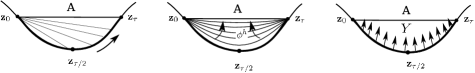
Figure 2: The isotopy $\psi_{h,\tau}^{s}$ and the vector field $Y$. Left: for every $0\leq\tau<\tau_{0}$ we have a different segment ${\bf A}$ joining ${\bf z}_{0}$ and ${\bf z}_{\tau}$. Center: for every fixed $\tau$ the parameter $h$ gives the isotopy $\phi^{h}$ between the segment ${\bf A}$ and the Hamiltonian flow. Right: the local vector field $Y$ generated by the isotopy on the segment ${\bf A}$.

Unfortunatelly, just the segments given by the values $\tau=0$ and $\tau=1$ in the parameterization (10) correspond to segments of Hamiltonian flows.

We are looking for an isotopy $\phi^{h}:[0,1]\times M\to M$ that, written as a local map, must satisfies

$$\phi^{0}({\bf z}([0,\tau]))={\bf z}([0,\tau])\qquad{\rm and}\qquad\phi^{1}({\bf z}([0,\tau]))={\bf A}$$

and such that the intermediate curves for $h\in(0,1)$ are also segments of Hamiltonian flows. We claim that this isotopy exists but the solution for our problem is, in fact, much simpler. We will work with the Hamiltonian vector field $X_{H}$ and its pull-back by a local diffeomorphism $u\in{\rm Diff}(U)$ defined in an open set $U\subset M$ around the segment ${\bf z}_{[0,\tau]}$.

It is well-known that the pull-back of $X_{H}$ by a diffeomorphism $u:M\to M$ is given by $u^{*}X_{H}=(du)^{-1}\cdot X_{H}\circ u$ [11, 30]. Also, we know that $u^{*}X_{H}$ is a Hamiltonian vector field if $u$ is a symplectomorphism. In the case of a one-parameter group of diffeomorphisms $u_{t}:\mathbb{R}\times M\to M$ the pull-back of $X_{H}$ is given by

$$u_{t}^{*}X_{H}=(du_{-t})\cdot X_{H}\circ u_{t}.$$

Supose that the one parameter group $u_{t}$ has infinitesimal generator $Y$, then the pull-back of $X_{H}$ has infinitesimal generator

$$X=\left.\left(\frac{d}{dt}u_{t}^{*}X_{H}\right)\right|_{t=0}={\mathcal{L}}_{Y}X_{H}=[X_{H},Y].$$ (11)

Again, if $u_{t}$ is a one-parameter group of symplectomorphisms, then (11) is a Hamiltonian vector field with Hamiltonian function $\omega(X_{H},Y)=-dH(Y)$. Moreover, if $Y=X_{K}$ is Hamiltonian with Hamiltonian function $K$, then (11) has Hamiltonian function $\omega(X_{H},X_{K})=\{K,H\}$ which is the Poisson bracket of $H$ and $K$. We have the classical relation $[X_{H},X_{K}]=X_{\{K,H\}}$ which determines the Lie algebra isomorphism between functions and Hamiltonian vector fields. All this applies on the whole manifold $(M,\omega)$ which we consider as the global case.

In the local case, there are local symmetries that cannot be extended to the global case. They are given by the flow of some Liouville vector fields $Z$ whose flow $\phi^{h}_{Z}$ satisfies $(\phi^{h}_{Z})^{*}\omega=e^{h}\omega$. In the general case, the flow of $Z$ is non necesarily complet and we need to consider open neighborhoods $W$, big enough for including the source and target domains $W\subset\left(U\cap\phi^{h}_{Z}(U)\right)$, and small values of the parameter $h\in(-c,c)$ in the flow $\phi^{h}_{Z}$.

Lemma 4.1

The pull-back of a Hamiltonian vector field $X_{H}$ under the local flow $\phi^{h}_{Z}$ of a Liouville vector field $Z$ is a (local) Hamiltonian vector field $X_{\mathcal{A}}$, with Hamiltonian function $\mathcal{A}=({\mathcal{L}}_{Z}H-H)$.

Proof. It is just the application of (11) for the case where the flow has a Liouville vector field as infinitesimal generator

$$\left.\left(\frac{d}{dh}\left(\phi^{h}_{Z}\right)^{*}X_{H}\right)\right|_{h=0}={\mathcal{L}}_{Z}X_{H}=[X_{H},Z].$$ (12)

To prove that it is Hamiltonian, we check the contraction of the vector field with the symplectic form $\omega$, indeed

$$i_{[X_{H},Z]}\omega={\mathcal{L}}_{X_{H}}i_{Z}\omega-i_{Z}{\mathcal{L}}_{X_{H}}\omega={\mathcal{L}}_{X_{H}}\theta=-d({\mathcal{L}}_{Z}H-H).$$

Then we have a local function ${\mathcal{A}}={\mathcal{L}}_{Z}H-H$, and $[X_{H},Z]=X_{\mathcal{A}}$ is a Hamiltonian vector field locally defined around the solution curves of $X_{H}$. $\hfill\square$

Remark 3

When the Liouville vector field is the vertical one $\sum_{i}p_{i}\frac{\partial}{\partial p_{i}}$, and the Hamiltonian vector field is a natural mechanical system, the function $\mathcal{A}$ corresponds to the Lagrangian function $L=2T-H$, where $T$ is the kinetic energy.

Remark 4

Previous lemma is a purely local result in contrast to the global case considered by Theorem VI.2.8 in [9]. We conjecture that for Liouville fields that can be extended to the whole manifold, an additionnal first integral is concerned.

The last discussion shows that we can use the flow of a Liouville vector field for constructing the local Hamiltonian isotropy connecting the segment ${\bf A}$ with the Hamiltonian flow.

5 The geometrical meaning of the ${\bf b}$ matrix

As proved in [21] using generating functions, the map

$${\bf z}_{\tau}={\bf z}_{0}+\tau X_{H}(\bar{\bf z}),\qquad{\rm where}\qquad\bar{\bf z}={\textstyle{\frac{1}{2}}}({\bf z}_{0}+{\bf z}_{\tau})+\tau b({\bf z}_{\tau}-{\bf z}_{0})$$ (13)

where $b\in\mathbb{M}_{2n\times 2n}(\mathbb{R})$ is a Hamiltonian matrix, defines a symmetric, symplectic map for constructing a symplectic integrator. In [14, 16] this result was refined using Liouvillian forms, where the matrix $b$ is generalized to a $(1,1)$ tensor ${\bf b}$ on $M$, which corresponds to the closed (in fact to the exact) component of a Liouvillian form $\theta$ on $M$. Return to the Hamiltonian isotopy proposed in the last section and consider only the mid-point in the line segment ${\bf A}$. The point $\bar{\bf z}$ where the Hamiltonian vector field is evaluated in the implicit map (13), is the image of the mid-point ${\textstyle{\frac{1}{2}}}({\bf z}_{0}+{\bf z}_{\tau})$ under the symplectic map $\phi=(I-2{\bf b}_{\tau})^{-1}(I+2{\bf b}_{\tau})$, where ${\bf b}_{\tau}=\tau{\bf b}$, for enough small $\tau>0$. In this case, ${\bf b}_{\tau}$ is non-exceptional and $\phi$ is well defined, moreover $\phi$ is close to the identity map.

We construct the symplectic isotopy $\phi_{h}:[0,1]\to Sp(M,\omega)$ connecting the mid-point ${\textstyle{\frac{1}{2}}}({\bf z}_{0}+{\bf z}_{\tau})$ with $\bar{\bf z}$ using the parameter $h$ by

$$\phi_{h}=(I-h2{\bf b}_{\tau})^{-1}(I+h2{\bf b}_{\tau}),\qquad h\in[0,1].$$ (14)

It satisfies $\phi_{0}=id$ and $\phi_{1}=\phi$, and it defines a symplectic map for each fixed $h\in[0,1]$. Moreover, since it is close to the identity, it is a Hamiltonian isotopy for some 1-parameter family of Hamiltonian functions $H_{t}:[0,1]\times M\to\mathbb{R}$ [26]. Since $\phi$ is symplectic for every ${\bf b}$ close to the zero tensor, the implicit map (13) corresponds to the exact discretization of the flow of the Hamiltonian function $H\circ\phi:M\to\mathbb{R}$ known in the numerical community as the “sourrounding Hamiltonian”. To be more specific, the symplectic mid-point scheme exactly integrates a “surrounding Hamiltonian” $\bar{H}=H\circ\varphi$ with equations of motion $\dot{\zeta}=X_{H\circ\varphi}(\zeta)$. Consequently, the map (13) integrates exactly the system

$$\dot{\zeta}=X_{H\circ\varphi\circ\phi}(\zeta).$$ (15)

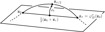
Figure 3: The Hamiltonian isotopy $\phi_{h}=(I-h2{\bf b}_{\tau})^{-1}(I+h2{\bf b}_{\tau})$, taking the mid-point to a point close to ${\bf z}_{\tau/2}$.

The goal is to find the local symplectic map $\phi$ approximating $\varphi^{-1}$. Equivalently, we search for the ${\bf b}$ tensor whose induced symplectic map $\phi$ takes the mid-point to some point on the solution we are integrating. If it is possible, $\phi^{-1}$ maps such a point on the mid-point, cancelling the numerical oscillations. Before to propose some approaches for the search of the ${\bf b}$ tensor, we will check the numerical algorithm.

6 The symplectic integrator

We consider the flow $\varphi^{t}_{H}$ of the Hamiltonian vector field $\dot{\bf z}=X_{H}({\bf z})$ and we integrate it in time from the initial condition ${\bf z}_{0}$

$$\int_{0}^{\tau}\frac{d}{dt}\varphi_{H}^{t}({\bf z}_{0})dt=\int_{0}^{\tau}X_{H}(\varphi_{H}^{t}({\bf z}_{0}))dt,\qquad{\bf z}_{0}\in M,\quad\forall\tau\in I,$$ (16)

where $I=(-\tau_{0},\tau_{0})$ for small $\tau_{0}\in\mathbb{R}$. Applying the fundamental theorem of calculus and reparameterizing the time by $s(t)=\frac{1}{\tau}t$ we have

$${\bf z}_{\tau}={\bf z}_{0}+\tau\int_{0}^{1}X_{H}(\varphi_{H}^{\tau s}({\bf z}_{0}))ds,\qquad\forall\tau\in I\subset\mathbb{R},$$ (17)

which is the integral version of equation $\dot{\bf z}=X_{H}({\bf z})$). For small $\tau$, which is the case here, expression (17) corresponds to the exponential map ${\bf z}_{\tau}=e^{\tau X_{H}}{\bf z}_{0}$.

The Cauchy-Lipschitz’s theorem (a.k.a. Picard-Lindelöf’s theorem) assures that a local solution for this equation always exists. Moreover, one way to approximate the value of ${\bf z}_{\tau}$ is by means of Picard iterations. Given a first guess ${\bf z}^{1}$ close to ${\bf z}_{\tau}$ the iterative scheme

$${\bf z}^{n+1}={\bf z}_{0}+\int_{0}^{\tau}X_{H}({\bf z}^{n}(s))ds,$$ (18)

approximates the value ${\bf z}_{\tau}$. The Picard-Lindelöf’s theorem assures the convergence of this iterative process for small $\tau$. Note that for big values of $\tau$, the Lipschitz condition cannot be fulfilled.

Consider a symplectic integrator given by Picard iterations [14]. Computing a first guess using an explicit scheme ${\bf z}^{1}=EulerA({\bf z}_{0})$, we iterate

$$\bar{\bf z} = {\textstyle{\frac{1}{2}}}({\bf z}_{0}+{\bf z}^{n})+\tau{\bf b}({\bf z}^{n}-{\bf z}_{0})$$ (19)

$${\bf z}^{n+1} = {\bf z}_{0}+\tau X_{H}(\bar{\bf z}).$$ (20)

This induces the following iterative algorithm:

Algorithm 1.
	$!$Setup the initial guess for ${\bf z}_{n+1}$
1:	${\bf z}^{[0]}={\bf z}_{n}+\tau X_{H}({\bf z}_{n})$
2:	for $j=0:\kappa$ do
	$!$ compute the tensor ${\bf b}$ at the mid-point
3:	$\quad b={\bf b}\left({\textstyle{\frac{1}{2}}}({\bf z}_{n}+{\bf z}^{[j]})\right)$
	$!$ compute the point $\bar{\bf z}$
4:	$\quad\bar{{\bf z}}={\textstyle{\frac{1}{2}}}({\bf z}_{n}+{\bf z}^{[j]})+\tau b({\bf z}^{[j]}-{\bf z}_{n})$
	$!$ refine the guess
5:	${\bf z}^{[j+1]}={\bf z}_{n}+\tau X_{H}(\bar{\bf z})$
6:	end for
7:	${\bf z}_{n+1}={\bf z}^{[\kappa]}$

The challenge is to find the way to compute, for a prescribed Hamiltonian system, a good guess of ${\bf b}$ depending in addition on the parameter $\tau$. We can consider the value of $\bar{\bf z}$ given in (19) as a first order approximation in $\tau$, and develop the tensor $\hat{\bf b}$ as a series in even powers of $\tau$ as follows

$$\hat{\bf b}={\bf b}_{0}+\tau^{2}{\bf b}_{2}+\tau^{4}{\bf b}_{4}+\cdots$$ (21)

where ${\bf b}_{j}$, $j=2k$ are symmetric, Hamiltonian $(1,1)$-tensors. Inserting (21) in (19) the symmetry $(\tau,{\bf z}_{0},{\bf z}_{\tau})\mapsto(-\tau,{\bf z}_{\tau},{\bf z}_{0})$ is preserved and the integrator preserves symmetry and symplecticity.

6.1 Looking forward the associated Liouvillian form

We have shown that the path that takes the mid-point to the point $\bar{\bf z}$ given in (13) is a Hamiltonian isotopy. This isotopy is attached to the Liouvillian form $\theta$ which defines the map. On the other hand, in contrast to the symplectic form $\omega$ which is preserved by the Hamiltonian flow $\varphi^{t}_{H}$, a Liouvillian form is not preserved, but it produces a Hamiltonian isotopy $dF_{t}:=(\varphi^{t}_{H})^{*}\theta-\theta$ which is related to the previous isotopy but they are not the same. We want to find a Liouvillian form induced by the geometry of the Hamiltonian system $(M,\omega,X_{H})$, such that its Liouville vector field determines an infinitesimal generator on a prescribed solution which sends it into another local solution but only in a tubular neighborhood.

The solution to this problem is adapted from an equivalent problem in the interface of contact and symplectic topologies. In the terminology used by McDuff and Salamon [26] it concerns the internal symplectization of a contact manifold. This procedure in addition, imposes a constraint concerning the lenght of the segment of Hamiltonian flow where the method works. In fact, this constraint comes from Gromov’s non-squeezing theorem [8] and it is related to the symplectic width of the “symplectized manifold”. This explains why Ge and Marsden’s lemma [7] on the reparameterization of the Hamiltonian flow is not a sufficient condition (among others assumptions) for claiming the non existence of energy preserving symplectic integrators.

The procedure to find a Liouvillian form for $(M,\omega,X_{H})$ works for regular solutions, i.e. for solutions belonging to a regular level hypersurface. The interested readers are refered to [11, 26, 35] for the generic construction, and [16] for the procedure adapted to a prescribed Hamiltonian system. In this paper we will only sketch the global procedure. It can be explained in two big steps.

The first step consists in to define a contact structure on the regular hypersurface fixed by the initial condition ${\bf z}_{0}$, leading to a contact manifold embedded in $(M,\omega)$. For this, fix the level hypersurface using the initial condition ${\bf z}_{0}\in M$ with regular value $H({\bf z}_{0})=h_{0}\in\mathbb{R}$. The set $\Sigma_{h}=H^{-1}(h_{0})$ is a smooth submanifold of codimension 1 by Saard’s theorem. Select a Liouville vector field $Z$ on $(M,\omega)$ which is transversal to $\Sigma_{h}$ and regular in a tubular neighborhood $U\subset M$ around $\Sigma_{h}$. Consider $\Sigma_{h}\subset U$ as an embedding $\jmath:\Sigma_{h}\to U$, and define the linear form $\alpha=\jmath^{*}\theta$ on $\Sigma_{h}$, which is the pullback of the Liouvillian form $\theta=i_{Z}\omega$ to $\Sigma_{h}$. We consider the distribution $\mathcal{D}=\ker(\alpha)$ which endows $\Sigma_{h}$ with a contact structure. $(\Sigma_{h},\mathcal{D})$ becomes a contact manifold with contact form $\alpha$. Finally, we define a Reeb field for $\alpha$ from the Hamiltonian vector field restricted to $\Sigma_{h}$ given by $R_{\alpha}=\frac{1}{\alpha(X_{H}|_{\Sigma})}X_{H}|_{\Sigma}$. Note that $R_{\alpha}$ is a rescaling of the Hamiltonian vector field and it depends on the selected vector field $Z$.

The second step is the internal symplectization which can be splitted in two parts: 1) the external symplectization, mapping $(\Sigma_{h},\alpha)\to(\Sigma_{h}\times\mathbb{R},d(e^{s}\alpha))$ and 2) the embedding of a slice around $\Sigma_{h}$ into the tubular neighborhood $U$, in this way $(\Sigma_{h}\times(-c,c),d(e^{s}\alpha))\to(U,d(\theta_{H,h}))$. Note that it is not necessary that $Z$, $\theta$ or $\theta_{H,h}$ be global forms, it suffies their regularity in the tubular neighborhood $\Sigma_{h}\subset U$. The difficulty in passing from the external to the internal symplectization is the construction of the Liouvillian form $\theta_{H,h}$ from $e^{s}\alpha$. It is a classical procedure obtained by using Weinstein’s proof of Darboux’s theorem, Moser’s trick and the homotopy lemma [26, 23, 11, 35].

The following expression is proved in [16]: The Liouvillian form $\theta_{H,h}$ associated to the Hamiltonian $H:M\to\mathbb{R}$ at the hypersurface level $h=H({\bf z}_{0})$ is given by

$$\theta_{H,h}=e^{h-H}\pi^{*}\alpha+\Phi(\varpi)$$ (22)

where

$$\varpi=\left(1-e^{h-H}\right)\omega+e^{h-H}dH\wedge\theta$$

is a closed 2-form which vanishes on $\Sigma_{h}$, and $\Phi(\varpi)$ is its cochain homotopy

$$\Phi(\varpi)=\int_{0}^{1}(\psi^{*}_{s}(i_{X_{s}}\varpi))ds\qquad{\rm where}\qquad X_{s}=\frac{s}{\|\nabla H\|^{2}}\nabla H,$$ (23)

and $\psi_{s}$ is the flow of the rescaled gradient $X_{s}$.

Once the Liouvillian form $\theta_{H,h}$ was computed, we extract the symmetric part which belongs to the kernel of the differential $d\theta_{H,h}=\omega$. Just for simplicity, we consider local coordinates $\{z_{i}\}_{i=1}^{2n}$ on $(M,\omega)$, related to Darboux’s coordinates by $(q_{i},p_{i})=(z_{i},z_{n+i}),i=1,...,n$. The Liouvillian form has a local expression in these coordinates by $\theta_{H,h}=\sum_{i}\alpha_{i}(z)dz_{i}$, where $\alpha_{i}:M\to\mathbb{R}$ are smooth functions. The closed part of $\theta_{H,h}$ is given by the symmetric matrix $S=(S_{ij})$ with expression

$$S_{ij}={\textstyle{\frac{1}{2}}}\left(\frac{\partial\alpha_{i}}{\partial z_{j}}+\frac{\partial\alpha_{j}}{\partial z_{i}}\right).$$ (24)

Finally we obtain a tensor $\tilde{\bf b}$ which contains the information of the Hamiltonian flow at the energy level $H({\bf z}_{0})=h$ by $\tilde{\bf b}=JS$, where $J$ is the complex structure associated to $\omega$. Inserting $\tilde{\bf b}$ into (19) we obtain a symplectic integrator adapted for simulating the flow $\varphi^{t}_{H}$ of the Hamiltonian vector field $X_{H}$ with initial condition ${\bf z}_{0}$.

The tensor ${\bf b}$ which minimizes the oscillations is related to $\theta_{H,h}=i_{(Z_{H},h)}\omega$, since the Liouville vector field $Z_{H,h}$ is the infinitesimal generator of the Hamiltonian isotopy connecting the continuous flow with the mid-point numerical approximation. This relation between ${\bf b}$ and $\theta_{H,h}$ can be highly non-linear. In a future it can be interesting to study this problem from the variational point of view.

7 Conclusions and perspectives

In this paper we refined the numerical scheme introduced in [14] and we collected a series of results to give a full geometrical explanation of the method of Liouvillian forms with application to symplectic integration. The geometric approach gives an intuitive framework for understanding the oscillatory behaviour of the numerical solution produced by a symplectic integrator when simulating Hamiltonian dynamics. A symplectic integrator defines intrinsically a Liouville vector field $Z$ and visceversa. The oscillations correspond to the projection of $Z$ on the gradient vector field $\nabla H$. This is

$$\langle Z,\nabla H\rangle=dH(Z)=\omega(Z,X_{H})=\theta(X_{H})$$

At first sight the method looks cryptic and abstract since the technique for finding the Liouvillian form associated to a prescribed Hamiltonian is difficult to visualize. However, this method shows that there is no local obstruction for approximating the separation of the numerical solution with respect to the continuous solution.

We obtain a framework which extends the method of generating functions giving an algorithmic way for constructing a symplectic map for approximating the flow of (almost) any generic, natural and classical Hamiltonian system. The use of a quaternionic structure on the product symplectic manifold simplifies the framework of special symplectic manifolds and gives a geometrical explanation to the Hamiltonian matrix $b$, first studied by Feng Kang as a condition for constructing implicit symplectic maps [21]. The quaternionic structure shows the relation between four objects: 1) the $b$ matrix which extends to the ${\bf b}$ tensor in this framework, 2) the Liouvillian form where the symmetric part $S$ of its diferential induces ${\bf b}=JS$, 3) the element $\bar{\bf z}={\textstyle{\frac{1}{2}}}({\bf z}_{0}+{\bf z}_{\tau})+{\bf b}({\bf z}_{\tau},{\bf z}_{0})$ which is interpreted as a tangent vector to the Lagrangian submanifold containing the flow, and 4) the symplectic map $\phi=(I-2{\bf b})^{-1}(1+2{\bf b})$ which is the (symplectic) Cayley transformation of ${\bf b}$ [17]. Moreover, if the “surrounding Hamiltonian” of the mid-point rule is $\bar{H}=H\circ\varphi$ then the “surrounding Hamiltonian” of this symplectic integrator is $\hat{H}=H\circ\varphi\circ\phi$. The challenge is to approximate the map $\varphi^{-1}$ in order to approximate the original function $H$.

Once the relationship between the Liouvillian form, the symplectic map and the symplectic integrator is given, we search for a suitable tensor ${\bf b}$ for inserting in the numerical scheme. Fortunatelly, there is a rich theory for the search of closed characteristics on compact contact type manifolds concerning a celebrated conjecture stated by Weinstein [11]. One of the main tools for solving this conjecture is the construction of a Liouville vector field, which is transversal to the contact type manifold at every point. We adapt this technique for a prescribed Hamiltonian system and we construct the Liouvillian form $\theta_{H,h}$ in a tubular neighborhood around the level hypersurface which contains the initial condition. This procedure is developed with all the details in [16]. This closes the loop relating the Hamiltonian system (with a given initial condition ${\bf z}_{0}$), the Liouvillian form, the ${\bf b}$ tensor and the symplectic integrator.

Remark 5

Note that the Liouvillian form $\theta_{H,h}$ depends on the Hamiltonian $H$ and, must important, it depends explicitly on the value $h=H({\bf z}_{0})$. For Hamiltonians with no other first integral and for chaotic systems, different values $h$ and $h+\epsilon$, for small $0<\epsilon\ll 1$, produce different Liouvillian forms.

A systematic study on numerical techniques for approximating the tensor ${\bf b}$, must be put in practice. In addition, it is necessary to search for a practical way of computing ${\bf b}$ without computing the integral expression of the cochain homotopy in the Liouvillian form (22). An alternative that we will study in the future is the approximation of the tensor ${\bf b}$ using variational methods.

References

- [1] R. Abraham and J.E. Marsden. Foundations of mechanics Second Ed. Benjamin Cummings, 1978.
- [2] V.I. Arnold. Mathematical Methods of Classical Mechanics 2nd. Ed. Springer-Verlag, 1989.
- [3] M. Chaperon. On generating families. In H. Hofer, C.H. Taubes, A. Weinstein, and E. Zehnder, editors, The Floer Memorial Volume, . Birkhäuser, 1995.
- [4] F. Kang. Difference schemes for Hamiltonian Formalism and Symplectic Geometry. J. Comput. Math., 4:279–289, 1985.
- [5] F. Kang and Z. Ge. On the approximation of Linear Hamiltonian Systems. J. Comput. Math., 6:88–97, 1988.
- [6] Z. Ge and W. Dau-liu. On the invariance of generating functions for symplectic transformations. Diff. Geom. and its Appl, 5:59–69, 1995.
- [7] Z. Ge and J. Marsden. Lie-Poisson Hamilton-Jacobi theory and Lie-Poisson integrators. Phys. Let. A, 133:134–139, 1988.
- [8] Misha Gromov. Soft and hard symplectic geometry. Proc. Int. Congress Math., pages 81–98, 1986.
- [9] E. Hairer, C. Lubich, and G. Wanner. Geometric Numerical Integration, Structure-Preserving Algorithms for Ordinary Differential Equations 2nd. Ed. Springer-Verlag, 2nd ed. edition, 2010.
- [10] Sir William Rowan Hamilton. On a General Method of Expressing the Paths of Light, & of the Planets, by the Coefficients of a Characteristic Function. PD Hardy Dublin, 1833.
- [11] Helmut Hofer and Eduard Zehnder. Symplectic invariants and Hamiltonian dynamics, rep 1994. Birkhäuser, 2012.
- [12] L. Hörmander. Fourier integral operators I. Acta Math., 127:79–183, 1971.
- [13] Carl Gustav Jacob Jacobi. Vorlesungen über dynamik, gesammelte werke, vol. VIII, Supplement, pages 221–231, 1884.
- [14] H. Jiménez-Pérez. Symplectic maps: from generating functions to Liouvillian forms. preprint, arxiv:1508.03250, 2015.
- [15] H. Jiménez-Pérez. Hamilton-Liouville pairs. preprint, 2016.
- [16] H. Jiménez-Pérez. Symplectic Integrators from Liouvillian Forms I: The Theoretical Framework. preprint, 2018.
- [17] H. Jiménez-Pérez. A Quaternionic Structure as Landmark For Symplectic Maps. preprint, 2019.
- [18] H. Jiménez-Pérez, J.P. Vilotte, and B. Romanowicz. New insights on numerical error in symplectic integration. preprint arXiv:1508.03303, 2015.
- [19] H. Jiménez-Pérez, J.P. Vilotte, and B. Romanowicz. On the Poincaré’s generating function and the symplectic mid-point rule. submitted arxiv:1508.07743, 2017.
- [20] H. Jiménez-Pérez, J.P. Vilotte, and B. Romanowicz. The source of numerical oscillations in symplectic integration. preprint, 2017.
- [21] F. Kang and M. Qin. Symplectic Geometric Algorithms for Hamiltonian Systems. Springer-Verlag, 2012.
- [22] Paulette Libermann. On Liouville Forms. Poisson Geometry, Banach Center Publications, 51:151–164, 2000.
- [23] Paulette Libermann and Charles-Michel Marle. Symplectic Geometry and Analytical Mechanics. Ridel, 1987.
- [24] Jerry E. Marsden and Tudor S. Ratiu. Introduction to Mechanics and Symmetry. Springer-Verlag, 1999.
- [25] V.P. Maslov. Theorie des perturbations et methodes asymptotiques, (French version from the Russian edition published in 1965). Dunod, 1972.
- [26] Dusa McDuff and Dietmar Salamon. Introduction to symplectic topology. Oxford University Press, 2017.
- [27] S. Morita. Geometry of Differential Forms. Iwanami series in modern mathematics. American Mathematical Society, 2001.
- [28] H. Poincaré. Les méthodes nouvelles de la mécanique céleste Tome III, volume III. Gauthier-Villars, 1899.
- [29] C. L. Siegel. Symplectic Geometry. Academic Press, 1964.
- [30] Shlomo Sternberg. Curvature in mathematics and physics. Dover Publications, 2013.
- [31] W.M. Tulczyjew. The Legendre Transformation. Annales de l’IHP, section A:1, 101-114.
- [32] W.M. Tulczyjew. Les sous-variétés lagrangiennes et la dynamique lagrangienne. C.R.Acad.Sci. Paris, 283:675–678, 1976.
- [33] Claude Viterbo. Symplectic topology as the geometry of generating functions. Mathematische Annalen, 292:685–710, 1992.
- [34] A. Weinstein. The invariance of Poincaré’s generating function for canonical transformations. Inventiones mathematicae, 16:202–213, 1972.
- [35] Alan Weinstein. Symplectic manifolds and their lagrangian submanifolds. Advances in Mathematics, 6(3):329 – 346, 1971.