Finding Near-Optimal Independent Sets at Scale

Abstract

The independent set problem is NP-hard and particularly difficult to solve in large sparse graphs. In this work, we develop an advanced evolutionary algorithm, which incorporates kernelization techniques to compute large independent sets in huge sparse networks. A recent exact algorithm has shown that large networks can be solved exactly by employing a branch-and-reduce technique that recursively kernelizes the graph and performs branching. However, one major drawback of their algorithm is that, for huge graphs, branching still can take exponential time. To avoid this problem, we recursively choose vertices that are likely to be in a large independent set (using an evolutionary approach), then further kernelize the graph. We show that identifying and removing vertices likely to be in large independent sets opens up the reduction space—which not only speeds up the computation of large independent sets drastically, but also enables us to compute high-quality independent sets on much larger instances than previously reported in the literature.

1 Introduction

The maximum independent set problem is an NP-hard problem that has attracted much attention in the combinatorial optimization community, due to its difficulty and its importance in many fields. Given a graph $G=(V,E)$, the goal of the maximum independent set problem is to compute a maximum cardinality set of vertices $\mathcal{I}\subseteq V$, such that no vertices in $\mathcal{I}$ are adjacent to one another. Such a set is called a maximum independent set (MIS). The maximum independent set problem has applications spanning many disciplines, including classification theory, information retrieval, and computer vision [14]. Independent sets are also used in efficient strategies for labeling maps [18], computing shortest paths on road networks [26], (via the complementary minimum vertex cover problem) computing mesh edge traversal ordering for rendering [34], and (via the complementary maximum clique problem) have applications in biology [16], sociology [23], and e-commerce [43].

It is easy to see that the complement of an independent set $\mathcal{I}$ is a vertex cover $V\backslash\mathcal{I}$ and an independent set in $G$ is a clique in the complement graph $\overline{G}$. Since all of these problems are NP-hard [17], heuristic algorithms are used in practice to efficiently compute solutions of high quality on large graphs [2, 21]. However, small graphs with hundreds to thousands of vertices may often be solved in practice with traditional branch-and-bound methods [32, 33, 39], and medium-sized instances can be solved exactly in practice using reduction rules to kernelize the graph. Recently, Akiba and Iwata [1] used advanced reduction rules with a measure and conquer approach to solve the minimum vertex cover problem for medium-scale sparse graphs exactly in practice. Thus, their algorithm also finds the maximum independent set for these instances. However, none of these exact algorithms can handle huge sparse graphs. Furthermore, our experiments suggest that the quality of existing heuristic-based solutions tends to degrade at scale for inputs such as Web graphs and road networks. Therefore, we need new techniques to find high-quality independent sets in these graphs.

Our Results.

We develop a state-of-the-art evolutionary algorithm that computes large independent sets by incorporating advanced reduction rules. Our algorithm may be viewed as performing two functions simultaneously: (1) reduction rules are used to boost the performance of the evolutionary algorithm and (2) the evolutionary algorithm opens up the opportunity for further reductions by selecting vertices that are likely to be in large independent sets. In short, our method applies reduction rules to form a kernel, then computes vertices to insert into the final solution and removes their neighborhood (including the vertices themselves) from the graph so that further reductions can be applied. This process is repeated recursively, discovering large independent sets as the recursion proceeds. We show that this technique finds large independent sets much faster than existing local search algorithms, is competitive with state-of-the-art exact algorithms for smaller graphs, and allows us to compute large independent sets on huge sparse graphs, with billions of edges.

2 Preliminaries

2.1 Basic Concepts

Let $G=(V=\{0,\ldots,n-1\},E)$ be an undirected graph with $n=|V|$ nodes and $m=|E|$ edges. The set $N(v)=\left\{u\,:\,\left\{v,u\right\}\in E\right\}$ denotes the neighbors of $v$. We further define the neighborhood of a set of nodes $U\subseteq V$ to be $N(U)=\cup_{v\in U}N(v)\setminus U$, $N[v]=N(v)\cup\{v\}$, and $N[U]=N(U)\cup U$. A graph $H=(V_{H},E_{H})$ is said to be a subgraph of $G=(V,E)$ if $V_{H}\subseteq V$ and $E_{H}\subseteq E$. We call $H$ an induced subgraph when $E_{H}=\left\{\{u,v\}\in E\,:\,u,v\in V_{H}\right\}$. For a set of nodes $U\subseteq V$, $G[U]$ denotes the subgraph induced by $U$. The complement of a graph is defined as $\overline{G}=(V,\overline{E})$, where $\overline{E}$ is the set of edges not present in $G$. An independent set is a set $\mathcal{I}\subseteq V$, such that all nodes in $\mathcal{I}$ are pairwise nonadjacent. An independent set is maximal if it is not a subset of any larger independent set. The independent set problem is that of finding the maximum cardinality independent set among all possible independent sets. A vertex cover is a subset of nodes $C\subseteq V$, such that every edge $e\in E$ is incident to at least one node in $C$. The minimum vertex cover problem asks for the vertex cover with the minimum number of nodes. Note that the vertex cover problem is complementary to the independent set problem, since the complement of a vertex cover $V\setminus C$ is an independent set. Thus, if $C$ is a minimum vertex cover, then $V\setminus C$ is a maximum independent set. A clique is a subset of the nodes $Q\subseteq V$ such that all nodes in $Q$ are pairwise adjacent. An independent set is a clique in the complement graph.

A $k$-way partition of a graph is a division of $V$ into $k$ blocks of nodes $V_{1},\ldots,V_{k}$ such that $V_{1}\cup\cdots\cup V_{k}=V$ and $V_{i}\cap V_{j}=\emptyset$ for $i\neq j$. A balancing constraint demands that $\forall i\in\{1,\ldots,k\}:|V_{i}|\leq L_{\max}=(1+\epsilon)\left\lceil|V|/k\right\rceil$ for some imbalance parameter $\epsilon$. The objective is to minimize the total cut $\sum_{i<j}w(E_{ij})$ where $E_{ij}=\left\{\left\{u,v\right\}\in E\,:\,u\in V_{i},v\in V_{j}\right\}$. The set of cut edges is also called edge separator. The $k$-way node separator problem asks to find $k$ blocks ($V_{1},V_{2},\ldots,V_{k}$) and a separator $S$ that partitions $V$ such that there are no edges between the blocks. Again, a balancing constraint demands $|V_{i}|\leq(1+\epsilon)\left\lceil|V|/k\right\rceil$. The objective is to minimize the size $|S|$ of the separator. By default, our initial inputs will have unit edge and node weights.

2.2 Related Work

We now outline related work for the MIS problem, covering local search, evolutionary, and exact algorithms. We review in more detail techniques that are directly employed in this paper, particularly the local search algorithm by Andrade et al. [2] (ARW) and the evolutionary algorithm by Lamm et al. [28] (EvoMIS).

Local Search Algorithms.

There is a wide range of heuristics and local search algorithms for the maximum clique problem (see for example [6, 22, 20, 25, 31, 21]). They typically maintain a single solution and try to improve it by performing node deletions, insertions, and swaps, as well as plateau search. Plateau search only accepts moves that do not change the objective function, which is typically achieved through node swaps—replacing a node by one of its neighbors. Note that a node swap cannot directly increase the size of the independent set. A very successful approach for the maximum clique problem has been presented by Grosso et al. [21]. In addition to using plateau search, it applies various diversification operations and restart rules.

For the independent set problem, Andrade et al. [2] extended the notion of swaps to $(j,k)$-swaps, which remove $j$ nodes from the current solution and insert $k$ nodes. The authors present a fast linear-time implementation that, given a maximal solution, can find a $(1,2)$-swap or prove that no $(1,2)$-swap exists. One iteration of the ARW algorithm consists of a perturbation and a local search step. The ARW local search algorithm uses simple $2$-improvements or $(1,2)$-swaps to gradually improve a single current solution. The simple version of the local search iterates over all nodes of the graph and looks for a $(1,2)$-swap. By using a data structure that allows insertion and removal operations on nodes in time proportional to their degree, this procedure can find a valid $(1,2)$-swap in $\mathcal{O}(m)$ time, if it exists. A perturbation step, used for diversification, forces nodes into the solution and removes neighboring nodes as necessary. In most cases a single node is forced into the solution; with a small probability the number of forced nodes $f$ is set to a higher value ($f$ is set to $i+1$ with probability $1/2^{i}$). Nodes to be forced into a solution are picked from a set of random candidates, with priority given to those that have been outside the solution for the longest time. An even faster incremental version of the algorithm (which we use here) maintains a list of candidates, which are nodes that may be involved in $(1,2)$-swaps. It ensures a node is not examined twice unless there is some change in its neighborhood.

Evolutionary Algorithms.

An evolutionary algorithm starts with a population of individuals (in our case independent sets of the graph) and then evolves the population into different ones over several rounds. In each round, the evolutionary algorithm uses a selection rule based on fitness to select good individuals and combine them to obtain an improved child [19].

In the context of independent sets, Bäck and Khuri [3] and Borisovsky and Zavolovskaya [7] use fairly similar approaches. In both cases a classic two-point crossover technique randomly selects two crossover points to exchanged parts of the input individuals, which is likely to result in invalid solutions. Recently, Lamm et al. [28] presented a very natural evolutionary algorithm using combination operations that are based on graph partitioning and ARW local search. They employ the state-of-the-art graph partitioner KaHIP [36] to derive operations that make it possible to quickly exchange whole blocks of given independent sets. Experiments indicate superior performance than other state-of-the-art algorithms on a variety of instances.

We now give a more detailed overview of the algorithm by Lamm et al., which we use as a subroutine. It represents each independent set (individual) $\mathcal{I}$ as a bit array $s=\{0,1\}^{n}$ where $s[v]=1$ if and only if $v\in\mathcal{I}$. The algorithm starts with the creation of a population of individuals (independent sets) by using greedy approaches and then evolves the population into different populations over several rounds until a stopping criterion is reached. In each round, the evolutionary algorithm uses a selection rule based on the fitness of the individuals (in this case, the size of the independent set) in the population to select good individuals and combine them to obtain an improved child.

The basic idea of the combine operations is to use a partition of the graph to exchange whole blocks of solution nodes and use local search afterwards to turn the solution into a maximal one. We explain one of the combine operations based on 2-way node separators in more detail. In its simplest form, the operator starts by computing a 2-way node separator $V=V_{1}\cup V_{2}\cup S$ of the input graph. The separator $S$ is then used as a crossover point for the operation. The operator generates two children, $O_{1}=(V_{1}\cap\mathcal{I}_{1})\cup(V_{2}\cap\mathcal{I}_{2})$ and $O_{2}=(V_{1}\cap\mathcal{I}_{2})\cup(V_{2}\cap\mathcal{I}_{1})$. In other words, whole parts of independent sets are exchanged from the blocks $V_{1}$ and $V_{2}$ of the node separator. Note that the exchange can be implemented in time linear in the number of nodes. Recall that a node separator ensures that there are no edges between $V_{1}$ and $V_{2}$. Hence, the computed children are independent sets, but may not be maximal since separator nodes have been ignored and potentially some of them can be added to the solution. Therefore, the child is made maximal by using a greedy algorithm. The operator finishes with one iteration of the ARW algorithm to ensure that a local optimum is reached and to add diversification.

Once the algorithm computes a child it inserts it into the population and evicts the solution that is most similar to the newly computed child among those individuals of the population that have a smaller or equal objective than the child itself. We give an outline in Algorithm 1.

   create initial population $P$

   while stopping criterion not fulfilled

    select parents $\mathcal{I}_{1},\mathcal{I}_{2}$ from $P$

    combine $\mathcal{I}_{1}$ with $\mathcal{I}_{2}$ to create child $O$

    ARW local search+mutation on child $O$

    evict individual in population using $O$

   return the fittest individual that occurred

Algorithm 1 EvoMIS Evolutionary Algorithm with Local Search for the Independent Set Problem

Exact Algorithms.

As in local search, most work in exact algorithms has focused on the complementary problem of finding a maximum clique. The most efficient algorithms use a branch-and-bound search with advanced vertex reordering strategies and pruning (typically using approximation algorithms for graph coloring, MAXSAT [29] or constraint satisfaction). The current fastest algorithms for finding the maximum clique are the MCS algorithm by Tomita et al. [39] and the bit-parallel algorithms of San Segundo et al. [32, 33]. Furthermore, recent experiments by Batsyn et al. [5] show that these algorithms can be sped up significantly by giving an initial solution found through local search. However, even with these state-of-the-art algorithms, graphs on thousands of vertices remain intractable. For example, only recently was a difficult graph on 4,000 vertices solved exactly, requiring 39 wall-clock hours in a highly-parallel MapReduce cluster, and is estimated to require over a year of sequential computation [41]. A thorough discussion of many recent results in clique finding can be found in the survey of Wu and Hao [40].

The best known algorithms for solving the independent set problem on general graphs have exponential running time, and much research has be devoted to reducing the base of the exponent. The main technique is to develop rules to modify the graph, removing subgraphs that can be solved simply, which reduces the graph to a smaller instance. These rules are referred to as reductions. Reductions have been used to reduce the running time of the brute force $O(n^{2}2^{n})$ algorithm to the $O(2^{n/3})$ time algorithm of Tarjan and Trojanowski [38], and to the current best polynomial space algorithm with running time of $O(1.2114^{n})$ by Bourgeois et al. [8]. These algorithms apply reductions during recursion, only branching when the graph can no longer be reduced [15].

Reduction techniques have been successfully applied in practice to solve exact problems that are intractable with general algorithms. Butenko et al. [9] were the first to show that simple reductions could be used to solve independent set problems on graphs with several hundred vertices for graphs derived from error-correcting codes. Their algorithm works by first applying isolated clique removal reductions, then solving the remaining graph with a branch-and-bound algorithm. Later, Butenko and Trukhanov [10] further showed that applying a critical set reduction technique could be used to solve graphs produced by the Sanchis graph generator.

Repeatedly applying reductions as a preprocessing step to produce an irreducible kernel graph is a technique that is often used in practice, and has been used to develop fixed-parameter tractable algorithms, parameterized on the kernel size. As for using reductions in branch-and-bound recursive calls, it has long been known that two such simple reductions, called pendant vertex removal and vertex folding, are particularly effective in practice. Recently, Akiba and Iwata [1] have shown that more advanced reduction rules are also highly effective, finding exact minimum vertex covers (and by extension, exact MIS) on a corpus of large social networks with hundreds of thousands of vertices or more in mere seconds. More details on the reduction rules follow in Section 3.

3 Algorithmic Components

We now discuss the main contributions of this work. To be self-contained, we begin with a rough description of the reduction rules that we employ from previous work and then describe the main algorithm, together with an additional augmentation to speed up the basic approach.

3.1 Kernelization

We now briefly describe the reductions used in our algorithm, in order of increasing complexity. Each reduction allows us to choose vertices that are in some MIS by following simple rules. If an MIS is found on the kernel graph $\mathcal{K}$, then each reduction may be undone, producing an MIS in the original graph. Refer to Akiba and Iwata [1] for a more thorough discussion, including implementation details. We use our own implementation of the reduction algorithms in our method.

Pendant vertices: Any vertex $v$ of degree one, called a pendant, is in some MIS; therefore $v$ and its neighbor $u$ can be removed from $G$.

Vertex folding: For a vertex $v$ with degree 2 whose neighbors $u$ and $w$ are not adjacent, either $v$ is in some MIS, or both $u$ and $w$ are in some MIS. Therefore, we can contract $u$, $v$, and $w$ to a single vertex $v^{\prime}$ and decide which vertices are in the MIS later.

Linear Programming: A well-known [30] linear programming relaxation for the MIS problem with a half-integral solution (i.e., using only values 0, 1/2, and 1) can be solved using bipartite matching: maximize $\sum_{v\in V}{x_{v}}$ such that $\forall(u,v)\in E$, $x_{u}+x_{v}\leq 1$ and $\forall v\in V$, $x_{v}\geq 0$. Vertices with value 1 must be in the MIS and can thus be removed from $G$ along with their neighbors. We use an improved version [24] that computes a solution whose half-integral part is minimal.

Unconfined [42]: Though there are several definitions of unconfined vertex in the literature, we use the simple one from Akiba and Iwata [1]. A vertex $v$ is unconfined when determined by the following simple algorithm. First, initialize $S=\{v\}$. Then find a $u\in N(S)$ such that $|N(u)\cap S|=1$ and $|N(u)\setminus N[S]|$ is minimized. If there is no such vertex, then $v$ is confined. If $N(u)\setminus N[S]=\emptyset$, then $v$ is unconfined. If $N(u)\setminus N[S]$ is a single vertex $w$, then add $w$ to $S$ and repeat the algorithm. Otherwise, $v$ is confined. Unconfined vertices can be removed from the graph, since there always exists an MIS $\mathcal{I}$ that contains no unconfined vertices.

Twin [42]: Let $u$ and $v$ be vertices of degree 3 with $N(u)=N(v)$. If $G[N(u)]$ has edges, then add $u$ and $v$ to $\mathcal{I}$ and remove $u$, $v$, $N(u)$, $N(v)$ from $G$. Otherwise, some vertices in $N(u)$ may belong to some MIS $\mathcal{I}$. We still remove $u$, $v$, $N(u)$ and $N(v)$ from $G$, and add a new gadget vertex $w$ to $G$ with edges to $u$’s two-neighborhood (vertices at a distance 2 from $u$). If $w$ is in the computed MIS, then none of $u$’s two-neighbors are $\mathcal{I}$, and therefore $N(u)\subseteq\mathcal{I}$. Otherwise, if $w$ is not in the computed MIS, then some of $u$’s two-neighbors are in $\mathcal{I}$, and therefore $u$ and $v$ are added to $\mathcal{I}$.

Alternative: Two sets of vertices $A$ and $B$ are set to be alternatives if $|A|=|B|\geq 1$ and there exists an MIS $\mathcal{I}$ such that $\mathcal{I}\cap(A\cup B)$ is either $A$ or $B$. Then we remove $A$ and $B$ and $C=N(A)\cap N(B)$ from $G$ and add edges from each $a\in N(A)\setminus C$ to each $b\in N(B)\setminus C$. Then we add either $A$ or $B$ to $\mathcal{I}$, depending on which neighborhood has vertices in $\mathcal{I}$. Two structures are detected as alternatives. First, if $N(v)\setminus\{u\}$ induces a complete graph, then $\{u\}$ and $\{v\}$ are alternatives (a funnel). Next, if there is a cordless 4-cycle $a_{1}b_{1}a_{2}b_{2}$ where each vertex has at least degree 3. Then sets $A=\{a_{1},a_{2}\}$ and $B=\{b_{1},b_{2}\}$ are alternatives when $|N(A)\setminus B|\leq 2$, $|N(A)\setminus B|\leq 2$, and $N(A)\cap N(B)=\emptyset$.

Packing [1]: Given a non-empty set of vertices $S$, we may specify a packing constraint $\sum_{v\in S}x_{v}\leq k$, where $x_{v}$ is 0 when $v$ is in some MIS $\mathcal{I}$ and 1 otherwise. Whenever a vertex $v$ is excluded from $\mathcal{I}$ (i.e., in the unconfined reduction), we remove $x_{v}$ from the packing constraint and decrease the upper bound of the constraint by one. Initially, packing constraints are created whenever a vertex $v$ is excluded or included into the MIS. The simplest case for the packing reduction is when $k$ is zero: all vertices must be in $\mathcal{I}$ to satisfy the constraint. Thus, if there is no edge in $G[S]$, $S$ may be added to $\mathcal{I}$, and $S$ and $N(S)$ are removed from $G$. Other cases are much more complex. Whenever packing reductions are applied, existing packing constraints are updated and new ones are added.

   input graph $G=(V,E)$, solution size offset $\gamma$ (initially zero)

   global var best solution $\mathcal{S}$

  

   if $|V|=0$ then return

   else

    // compute exact kernel and intermediate solution

    $(\mathcal{K},\theta)\leftarrow$ computeExactKernel($G$) {exact kernel, solution size offset $\theta$}

    $\mathcal{I}\leftarrow$ EvoMIS($\mathcal{K}$) {intermediate independent set}

    if $|\mathcal{I}|+\gamma+\theta>|\mathcal{S}|$ then update $\mathcal{S}$

  

    // compute inexact kernel

    select $\mathcal{U}\subseteq\mathcal{I}$ s.t. $|\mathcal{U}|=\lambda$, $\forall u\in\mathcal{U},v\in\mathcal{I}\backslash\mathcal{U}:d_{\mathcal{K}}(u)\leq d_{\mathcal{K}}(v)$ {fixed vertices}

    $\mathcal{U}=\mathcal{U}\cup N(\mathcal{U})$ {augment $\mathcal{U}$ with its neighbors}

    $\mathcal{K}^{\prime}\leftarrow\mathcal{K}[V_{\mathcal{K}}\backslash\mathcal{U}]$ {inexact kernel}

  

    // recurse on inexact kernel

    ReduMIS($\mathcal{K}^{\prime}$, $\gamma+\theta+|\mathcal{U}|$) {recursive call with updated offsets}

   return $\mathcal{S}$

Algorithm 2 ReduMIS

3.2 Faster Evolutionary Computation of Independent Sets

Our algorithm applies the reduction rules from above until none of them is applicable. The resulting graph $\mathcal{K}$ is called the kernel. Akiba and Iwata [1] use a branch-and-reduce technique, first computing the kernel, then branching and recursing. Often the kernel $\mathcal{K}$ is empty, giving an exact solution without any branching. Depending on the graph structure, however, the kernel can be too large to be solved exactly (see Section 4). For several practical inputs, the kernel is still significantly smaller than the input graph. Furthermore, any solution of $\mathcal{K}$ can be extended to a solution of the input.

With these two facts in mind, we apply the evolutionary algorithm on $\mathcal{K}$ instead of on the input graph, thus boosting its performance. We stop the evolutionary algorithm after $\mu$ unsuccessful combine operations and look at the best individual (independent set) $\mathcal{I}$ in the population. This corresponds to an intermediate solution to the input problem, whose size we can compute based on some simple bookkeeping (without actually reconstructing the full solution in $G$). Instead of stopping the algorithm, we use $\mathcal{I}$ to further reduce the graph and repeat the process of applying exact reduction rules and using the evolutionary algorithm on the further reduced graph $\mathcal{K}^{\prime}$ recursively.

Our inexact reduction technique opens up the reduction space by selecting a subset $\mathcal{U}$ of the independent set vertices of the best individual $\mathcal{I}$. These vertices and their neighbors are then removed from the kernel. Based on the intuition that high-degree vertices in $\mathcal{I}$ are unlikely to be in a large solution (consider for example the optimal independent set on a star graph), we choose the $\lambda$ vertices from $\mathcal{I}$ with the smallest degree as subset $\mathcal{U}$. Using a modified quick selection routine this can be done in linear time. Ties are broken randomly. It is easy to see that it is likely that some of the exact reduction techniques become applicable again. Another view on the inexact reduction is that we use the evolutionary algorithm to find vertices that are likely to be in a large independent set. The overall process is repeated until the newly computed kernel is empty or a time limit is reached. We present pseudocode in Algorithm 2.

Additional Acceleration.

We now propose a technique to accelerate separator-based combine operations, which are the centerpiece of the evolutionary portion of our algorithm. Recall that after performing a combine operation, we first use a greedy algorithm on the separator to maximize the child and then employ ARW local search to ensure that the output individual is locally optimal with respect to (1,2)-swaps (see Algorithm 1). However, the ARW local search algorithm uses all independent set nodes for initialization. We can do better since large subsets of the created individual are already locally maximal (due to the nature of combine operations, which takes as input locally maximal individuals). It is sufficient to initialize ARW local search with the independent set nodes in the separator (added by the greedy algorithm) and the solution nodes adjacent to the separator.

4 Experimental Evaluation

Methodology.

We have implemented the algorithm described above using C++ and compiled all code using gcc 4.63 with full optimizations turned on (-O3 flag). Our implementation includes the reduction routines, local search, and the evolutionary algorithm. The exact algorithm by Akiba and Iwata [1] was compiled and run sequentially with Java 1.8.0_40. For the optimal algorithm, we mark the running time with a “-” when the instance could not be solved within ten hours, or could not be solved due to stack overflow. Unless otherwise mentioned, we perform five independent runs of each algorithm, where each algorithm is run sequentially with a ten-hour wall-clock time limit to compute its best solution. We use two machines for our experiments. Machine A is equipped with two Quad-core Intel Xeon processors (X5355) running at 2.667 GHz. It has 2x4 MB of level 2 cache each, 64 GB main memory and runs SUSE Linux Enterprise 10 SP 1. We use this machine in Section 4.1 for the instances taken from [28]. Machine B has four Octa-Core Intel Xeon E5-4640 processors running at 2.4 GHz. It has 512 GB local memory, 20 MB L3-Cache and 8x256 KB L2-Cache. We use this machine in Section 4.1 to solve the largest instances in our collection. We used the fastsocial configuration of the KaHIP v0.6 graph partitioning package [35] to obtain graph partitions and node separators necessary for the combine operations of the evolutionary algorithm. Experiments for the ARW algorithm, the exact algorithm, and the original EvoMIS algorithm were run on machine A. Data for ARW and EvoMIS are also found in [28], which uses the same machine.

We present two kinds of data: (1) the solution size statistics aggregated over the five runs, including maximum, average, and minimum values and (2) convergence plots, which show how the solution quality changes over time. Whenever an algorithm finds a new best independent set $S$ at time $t$, it reports a tuple ($t$, $|S|$); the convergence plots use average values over all five runs.

Algorithm Configuration.

After preliminary experiments, we fixed the convergence parameter $\mu$ to 1,000 and the inexact reduction parameter $\lambda$ to 0.1$\cdot|\mathcal{I}|$. However, our experiments indicate that our algorithm is not too sensitive to the precise choice of the parameters. Parameters of local search and other parameters of the evolutionary algorithm remain as in Lamm et al. [28]. We mark the instances that have been used for the parameter tuning here and in Appendix 0.A with a *.

Instances.

First, we conduct experiments on all instances used by Lamm et al. [28]. The social networks include citation networks, autonomous systems graphs, and Web graphs taken from the 10th DIMACS Implementation Challenge benchmark set [4]. Road networks are taken from Andrade et al. [2] and meshes are taken from Sander et al. [34]. Meshes are dual graphs of triangular meshes. Networks from finite element computations have been taken from Chris Walshaw’s benchmark archive [37]. Graphs derived from sparse matrices have been taken from the Florida Sparse Matrix Collection [11]. In addition, we perform experiments on huge instances with up to billions of edges. The graphs eu-2005, uk-2002, it-2004, sk-2005 and uk-2007 are Web graphs taken from the Laboratory of Web Algorithmics [27]. The graphs europe and usa-rd are large road networks of Europe [12] and the USA [13]. The instances as-Skitter-big, web-Stanford and libimseti are the hardest instances from Akiba and Iwata [1],

4.1 Solution Quality and Algorithm Performance

In this section, we compare solution quality and performance of our new reduction-based algorithm (ReduMIS) with the evolutionary algorithm by Lamm et al. [28] (EvoMIS), local search (ARW), and the exact algorithm by Akiba and Iwata [1]. We do this on the instances used in [28] and present detailed data in Appendix 0.A. We briefly summarize the main results of our experiments.

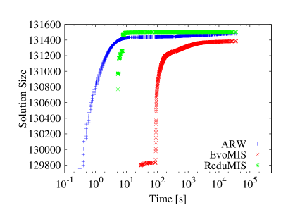
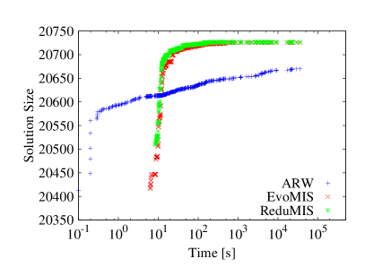
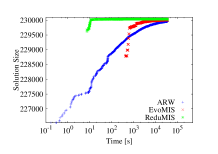
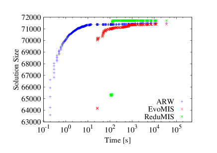
Figure 1: Convergence plots for ny (top left), gameguy (top right), cnr-2000 (bottom left), fe_ocean (bottom right).

First, ReduMIS always improves or preserves solution quality on social or road networks. On four social networks (cnr-2000, skitter, amazon and in-2004) and on all road networks, we compute a solution strictly larger than EvoMIS and ARW. On mesh-like networks, ReduMIS computes solutions which are sometimes better and sometimes worse than the previous formulation of the evolutionary algorithm; however, ARW performs significantly better than both algorithms on large meshes. (See representative results from experiments in Table 1.) EvoMIS reached its solution fairly late within the ten-hour time limit in the cases where ReduMIS computes a smaller solution than EvoMIS. This indicates that (1) increasing the patience/convergence parameter $\mu$ may improve the result on these networks and (2) it is harder to fix certain nodes into the solution since these networks contain many different independent sets. The convergence plots in Figure 1 show that the running time of the evolutionary algorithm is reduced with kernelization, especially on road and social networks. Once the first kernel is computed, ReduMIS quickly outperforms ARW and EvoMIS.

The exact algorithm performs as expected: it either quickly solves an instance (typically in a few seconds), or it cannot solve the instance within the ten-hour limit. Our experiments indicate that success of the exact algorithm is tied to the size of the first exact kernel. For most instances, if the kernel is too large the algorithm does not finish within the ten-hour time limit. Since the exact reduction rules work well for social networks and road networks, the algorithm can solve many of these instances. However, the exact algorithm cannot solve any mesh graphs and fails to solve many other instances, since reductions do not produce a small kernel on these instances. On all instances that the exact algorithm solved, our algorithm computes a solution having the same size; that is, each of our five runs computed an optimal result. In 29 out of 36 cases where the exact algorithm could not find a solution, the variance of the solution size obtained by the heuristics used here is greater than zero. Therefore, we consider these instances to be hard.

We present running times of the exact algorithm and our algorithm on the instances that the exact algorithm could solve in Appendix 0.A, Table 8. On most of the instances, the running times of both algorithms are comparable. Note, however, that our algorithm is not optimized for speed. For example, our evolutionary algorithm builds all the partitions needed for the combine operations when the algorithm starts. On some instances our algorithm outperforms the exact algorithm by far. The largest speed up is obtained bcsstk30, where our algorithm is about four orders of magnitude faster. Conversely, there are instances for which our algorithm needs much more time; for example, the instance Oregon-1 is solved 364 times faster by the exact algorithm.

Table 1: Results for representative social networks, road networks, Walshaw benchmarks, sparse matrix instances, and meshes from our experiments. Note that for the large mesh instance buddha, ReduMIS finds much smaller independent sets than ARW, since reductions do not effectively reduce large meshes.

Graph			ReduMIS			EvoMIS			ARW
Name	$n$	Opt.	Avg.	Max.	Min.	Avg.	Max.	Min.	Avg.	Max.	Min.
in-2004	1 382 908	896 762	896 762	896 762	896 762	896 581	896 585	896 580	896 477	896 562	896 408
cnr-2000	325 557	-	230 036	230 036	230 036	229 981	229 991	229 976	229 955	229 966	229 940
ny	264 346	-	131 502	131 502	131 502	131 384	131 395	131 377	131 481	131 485	131 476
fla	1 070 376	549 637	549 637	549 637	549 637	549 093	549 106	549 072	549 581	549 587	549 574
brack2	62 631	21 418	21 418	21 418	21 418	21 417	21 417	21 417	21 416	21 416	21 415
fe_ocean	143 437	-	71 706	71 716	71 667	71 390	71 576	71 233	71 492	71 655	71 291
GaAsH6	61 349	-	8 567	8 589	8 550	8 562	8 572	8 547	8 519	8 575	8 351
cant	62 208	-	6 260	6 260	6 259	6 260	6 260	6 260	6 255	6 255	6 254
bunny	68 790	-	32 346	32 348	32 342	32 337	32 343	32 330	32 293	32 300	32 287
buddha	1 087 716	-	480 072	480 104	480 043	478 879	478 936	478 795	480 942	480 969	480 921

Table 2: Results on huge instances. Value $n(\mathcal{K})$ denotes the number of nodes of the first exact kernel and $\overline{n}(\mathcal{K}^{\prime\prime})$ denotes the average number of nodes of the first inexact kernel (i. e., the number of vertices of the exact kernel of $\mathcal{K}^{\prime}$). Column $\ell$ presents the average recursion depth in which the best solution was found and $t_{\text{avg}}$ denotes the average time when the solution was found (including the time of the exact kernelization routines). A value of $\ell>1$ indicates that the best solution was not found on the exact kernel but on an inexact kernel during the course of the algorithm. Entries marked with a * indicate that ARW could not solve the instance.

graph	$n$	$m$	$n(\mathcal{K})$	$\overline{n}(\mathcal{K^{\prime\prime}}$)	Avg.	Max	$\ell$	$t_{\text{avg}}$	Max${}_{\text{ARW}}$
europe	$\approx$18.0M	$\approx$22.2M	11 879	826	9 267 810	9 267 811	1.4	2m	9 249 040
usa-rd	$\approx$23.9M	$\approx$28.8M	169 808	8 926	12 428 075	12 428 086	2.0	38m	12 426 262
eu-2005	$\approx$862K	$\approx$16.1M	68 667	55 848	452 352	452 353	1.4	26m	451 813
uk-2002	$\approx$19M	$\approx$261M	241 517	182 213	11 951 998	11 952 006	4.6	213m	*
it-2004	$\approx$41M	$\approx$1.0G	1 602 560	1 263 539	25 620 513	25 620 651	1.4	26.1h	*
sk-2005	$\approx$51M	$\approx$1.8G	3 200 806	2 510 923	30 686 210	30 686 446	1.4	27.3h	*
uk-2007	$\approx$106M	$\approx$3.3G	3 514 783	-	67 285 232	67 285 438	1.0	30.4h	*

Additional Experiments.

We now run our algorithm on the largest instances of our benchmark collection: road networks (europe, usa-rd) and Web graphs (eu-2005, uk-2002, it-2004, sk-2005 and uk-2007). For these experiments, we reduced the convergence parameter $\mu$ to 250 in order to speed up computation. On the three largest graphs it-2004, sk-2005 and uk-2007, we set the time limit of our algorithm to 24 hours after the first exact kernel has been computed by the kernelization routine. Table 2 gives detailed results of the algorithm including the size of the first exact kernel. We note that the first exact kernel is much smaller than the input graph: the reduction rules shrink the graph size by at least an order of magnitude. The largest reduction can be seen on the europe graph, for which the first kernel is more then three orders of magnitude smaller than the original graph. However, most of the kernels are still too large to be solved by the exact algorithm. As expected, applying our inexact reduction technique (i. e., fixing vertices into the solution and applying exact reductions afterwards) further reduces the size of the input graph. On road networks, inexact reductions reduce the graph size again by an order of magnitude. Moreover, the best solution found by our algorithm is not found on the first exact kernel $\mathcal{K}$, but in deeper recursion levels. In other words, the best solution found by our algorithm in one run is found on an inexact kernel. We run ARW on these instances as well, giving it as much time as our algorithm consumed to find its best solution. It could not handle the largest instances and computes smaller independent sets on the other instances.

We also ran our algorithm on the hardest instances computed exactly by Akiba and Iwata [1]: as-Skitter-big, web-Stanford, and libimseti. ReduMIS computes the optimal result on the instances as well. ReduMIS is a factor 147 and 2 faster than the exact algorithm on instances web-Stanford and as-Skitter-big respectively. However, we need a factor 16 more time for the libimseti instance.

5 Conclusion

In this work we developed a novel algorithm for the maximum independent set problem, which repeatedly kernelizes the graph until a large independent set is found. After applying exact reductions, we use a preliminary solution of the evolutionary algorithm to further reduce the kernel size by identifying and removing vertices likely to be in large independent sets. This further opens the reduction space (i. e., more exact reduction routines can be applied) so that we then proceed recursively. This speeds up computations drastically and preserves or even improves final solution quality. It additionally enables us to compute high quality independent sets on instances that are much larger than previously reported in the literature. In addition, our new algorithm computes an optimal independent set on all instances that the exact algorithm can solve.

Important future work includes a coarse-grained parallelization of our evolutionary approach, which can be done using an island-based approach, as well as parallelization of the reduction algorithms. Reductions and fixing independent set vertices can disconnect the kernel. Hence, in future work we want to solve each of the resulting connected components separately, perhaps also in parallel. Note that new reductions can be easily integrated into our framework. Hence, it may be interesting to include new exact reduction routines once they are discovered. Lastly, it may also be interesting to use an exact algorithm as soon as the graph size falls below a threshold.

Appendix 0.A Detailed per Instance Results

Table 3: Results for social networks.

Graph			ReduMIS			EvoMIS			ARW
Name	$n$	Opt.	Avg.	Max.	Min.	Avg.	Max.	Min.	Avg.	Max.	Min.
enron	69 244	62 811	62 811	62 811	62 811	62 811	62 811	62 811	62 811	62 811	62 811
gowalla	196 591	112 369	112 369	112 369	112 369	112 369	112 369	112 369	112 369	112 369	112 369
citation	268 495	150 380	150 380	150 380	150 380	150 380	150 380	150 380	150 380	150 380	150 380
cnr-2000*	325 557	-	230 036	230 036	230 036	229 981	229 991	229 976	229 955	229 966	229 940
google	356 648	174 072	174 072	174 072	174 072	174 072	174 072	174 072	174 072	174 072	174 072
coPapers	434 102	47 996	47 996	47 996	47 996	47 996	47 996	47 996	47 996	47 996	47 996
skitter	554 930	-	328 626	328 626	328 626	328 519	328 520	328 519	328 609	328 619	328 599
amazon	735 323	-	309 794	309 794	309 793	309 774	309 778	309 769	309 792	309 793	309 791
in-2004	1 382 908	896 762	896 762	896 762	896 762	896 581	896 585	896 580	896 477	896 562	896 408

Table 4: Results for mesh type graphs.

Graph			ReduMIS			EvoMIS			ARW
Name	$n$	Opt.	Avg.	Max.	Min.	Avg.	Max.	Min.	Avg.	Max.	Min.
beethoven	4 419	-	2 004	2 004	2 004	2 004	2 004	2 004	2 004	2 004	2 004
cow	5 036	-	2 346	2 346	2 346	2 346	2 346	2 346	2 346	2 346	2 346
venus	5 672	-	2 684	2 684	2 684	2 684	2 684	2 684	2 684	2 684	2 684
fandisk	8 634	-	4 074	4 075	4 073	4 075	4 075	4 075	4 073	4 074	4 072
blob	16 068	-	7 250	7 250	7 249	7 249	7 250	7 248	7 249	7 250	7 249
gargoyle	20 000	-	8 852	8 852	8 851	8 853	8 854	8 852	8 852	8 853	8 852
face	22 871	-	10 217	10 218	10 217	10 218	10 218	10 218	10 217	10 217	10 217
feline	41 262	-	18 853	18 854	18 851	18 853	18 854	18 851	18 847	18 848	18 846
gameguy	42 623	-	20 726	20 727	20 724	20 726	20 727	20 726	20 670	20 690	20 659
bunny*	68 790	-	32 346	32 348	32 342	32 337	32 343	32 330	32 293	32 300	32 287
dragon	150 000	-	66 438	66 449	66 433	66 373	66 383	66 365	66 503	66 505	66 500
turtle	267 534	-	122 417	122 437	122 383	122 378	122 391	122 370	122 506	122 584	122 444
dragonsub	600 000	-	281 561	281 637	281 509	281 403	281 436	281 384	282 006	282 066	281 954
ecat	684 496	-	322 363	322 419	322 317	322 285	322 357	322 222	322 362	322 529	322 269
buddha	1 087 716	-	480 072	480 104	480 043	478 879	478 936	478 795	480 942	480 969	480 921

Table 5: Results for Walshaw benchmark graphs.

Graph			ReduMIS			EvoMIS			ARW
Name	$n$	Opt.	Avg.	Max.	Min.	Avg.	Max.	Min.	Avg.	Max.	Min.
crack	10 240	4 603	4 603	4 603	4 603	4 603	4 603	4 603	4 603	4 603	4 603
vibrobox	12 328	-	1 852	1 852	1 851	1 852	1 852	1 852	1 850	1 851	1 849
4elt	15 606	-	4 943	4 944	4 942	4 944	4 944	4 944	4 942	4 944	4 940
cs4	22 499	-	9 167	9 168	9 166	9 172	9 177	9 170	9 173	9 174	9 172
bcsstk30	28 924	1 783	1 783	1 783	1 783	1 783	1 783	1 783	1 783	1 783	1 783
bcsstk31	35 588	3 488	3 488	3 488	3 488	3 488	3 488	3 488	3 487	3 487	3 487
fe_pwt	36 519	-	9 309	9 309	9 308	9 309	9 310	9 309	9 310	9 310	9 308
brack2	62 631	21 418	21 418	21 418	21 418	21 417	21 417	21 417	21 416	21 416	21 415
fe_tooth	78 136	27 793	27 793	27 793	27 793	27 793	27 793	27 793	27 792	27 792	27 791
fe_rotor	99 617	-	22 010	22 016	21 999	22 022	22 026	22 019	21 974	22 030	21 902
598a*	110 971	-	21 814	21 819	21 810	21 826	21 829	21 824	21 891	21 894	21 888
fe_ocean	143 437	-	71 706	71 716	71 667	71 390	71 576	71 233	71 492	71 655	71 291
wave	156 317	-	37 054	37 060	37 047	37 057	37 063	37 046	37 023	37 040	36 999
auto	448 695	-	83 873	83 891	83 846	83 935	83 969	83 907	84 462	84 478	84 453

Table 6: Results for road networks.

Graph			ReduMIS			EvoMIS			ARW
Name	$n$	Opt.	Avg.	Max.	Min.	Avg.	Max.	Min.	Avg.	Max.	Min.
ny*	264 346	-	131 502	131 502	131 502	131 384	131 395	131 377	131 481	131 485	131 476
bay	321 270	166 384	166 384	166 384	166 384	166 329	166 345	166 318	166 368	166 375	166 364
col	435 666	225 784	225 784	225 784	225 784	225 714	225 721	225 706	225 764	225 768	225 759
fla	1 070 376	549 637	549 637	549 637	549 637	549 093	549 106	549 072	549 581	549 587	549 574

Table 7: Results for graphs from Florida Sparse Matrix collection.

Graph			ReduMIS			EvoMIS			ARW
Name	$n$	Opt.	Avg.	Max.	Min.	Avg.	Max.	Min.	Avg.	Max.	Min.
Oregon-1	11 174	9 512	9 512	9 512	9 512	9 512	9 512	9 512	9 512	9 512	9 512
ca-HepPh	12 006	4 994	4 994	4 994	4 994	4 994	4 994	4 994	4 994	4 994	4 994
skirt	12 595	2 383	2 383	2 383	2 383	2 383	2 383	2 383	2 383	2 383	2 383
cbuckle	13 681	1 097	1 097	1 097	1 097	1 097	1 097	1 097	1 097	1 097	1 097
cyl6	13 681	600	600	600	600	600	600	600	600	600	600
case9	14 453	7 224	7 224	7 224	7 224	7 224	7 224	7 224	7 224	7 224	7 224
rajat07	14 842	4 971	4 971	4 971	4 971	4 971	4 971	4 971	4 971	4 971	4 971
Dubcova1	16 129	4 096	4 096	4 096	4 096	4 096	4 096	4 096	4 096	4 096	4 096
olafu	16 146	735	735	735	735	735	735	735	735	735	735
bodyy6	19 366	-	6 229	6 232	6 223	6 232	6 233	6 230	6 226	6 228	6 224
raefsky4	19 779	1 055	1 055	1 055	1 055	1 055	1 055	1 055	1 053	1 053	1 053
smt	25 710	-	782	782	782	782	782	782	780	780	780
pdb1HYS	36 417	-	1 077	1 078	1 076	1 078	1 078	1 078	1 070	1 071	1 070
c-57	37 833	19 997	19 997	19 997	19 997	19 997	19 997	19 997	19 997	19 997	19 997
copter2	55 476	-	15 192	15 194	15 191	15 192	15 195	15 191	15 186	15 194	15 179
TSOPF_FS_b300_c2	56 813	28 338	28 338	28 338	28 338	28 338	28 338	28 338	28 338	28 338	28 338
c-67	57 975	31 257	31 257	31 257	31 257	31 257	31 257	31 257	31 257	31 257	31 257
dixmaanl	60 000	20 000	20 000	20 000	20 000	20 000	20 000	20 000	20 000	20 000	20 000
blockqp1	60 012	20 011	20 011	20 011	20 011	20 011	20 011	20 011	20 011	20 011	20 011
Ga3As3H12	61 349	-	8 068	8 132	8 146	7 839	8 151	8 097	8 061	8 124	7 842
GaAsH6	61 349	-	8 567	8 589	8 550	8 562	8 572	8 547	8 519	8 575	8 351
cant	62 208	-	6 260	6 260	6 259	6 260	6 260	6 260	6 255	6 255	6 254
ncvxqp5*	62 500	-	24 504	24 523	24 482	24 526	24 537	24 510	24 580	24 608	24 520
crankseg_2	63 838	1 735	1 735	1 735	1 735	1 735	1 735	1 735	1 735	1 735	1 735
c-68	64 810	36 546	36 546	36 546	36 546	36 546	36 546	36 546	36 546	36 546	36 546

Table 8: Running times for ReduMIS and the exact algorithm on the graphs that the exact algorithm could solve. Running times $t_{\text{ReduMIS}}$ are average values of the time that the solution was found. Instances marked with a $\dagger$ are the hardest instances solved exactly in [1]. Running times in bold are those where ReduMIS found the exact solution significantly faster than the exact algorithm.

Graph	Opt.	$t_{\text{ReduMIS}}$	$t_{\text{exact}}$
a5esindl	30 004	0.07	0.07
as-Skitter-big†	1 170 580	1 262.46	2 838.030
bay	166 384	14.32	2.33
bcsstk30	1 783	2.71	31 152.16
bcsstk31	3 488	3.11	2.20
blockqp1	20 011	46.33	3.89
brack2	21 418	9.43	792.48
c-57	19 997	6.70	0.03
c-67	31 257	1.02	0.03
c-68	36 546	0.45	0.05
ca-HepPh	4 994	0.50	0.07
case9	7 224	3.23	0.54
cbuckle	1 097	3.83	1.34
citation	150 380	0.52	0.49
col	225 784	27.93	7 140.28
coPapers	47 996	3.21	1.45
crack	4 603	0.05	0.06
crankseg_2	1 735	1.86	2.63
cyl6	600	0.86	0.29
dixmaanl	20 000	12.27	13.62
Dubcova1	4 096	0.07	0.05
enron	62 811	3.08	0.06
fe_tooth	27 793	0.20	0.439
fla	549 637	20.10	22.50
in-2004	896 762	7.82	5.08
gowalla	112 369	0.79	0.33
libimseti†	127 294	28 375.4	1 729.05
olafu	735	3.84	1.44
Oregon-1	9 512	2.55	0.01
raefsky4	1 055	0.86	0.33
rajat07	4 971	0.02	0.05
skirt	2 383	0.14	0.14
TSOPF_FS_b300_c2	28 338	139.25	32.83
web-Google	174 072	2.95	0.83
web-Stanford†	163 390	316.15	46 450.11

References

- [1] T. Akiba and Y. Iwata. Branch-and-reduce Exponential/FPT Algorithms in Practice: A Case Study of Vertex Cover. In Proceedings of the Meeting on Algorithm Engineering & Expermiments, ALENEX ’15, pages 70–81, Philadelphia, PA, USA, 2015. Society for Industrial and Applied Mathematics.
- [2] D. V. Andrade, M. G. C. Resende, and R. F. Werneck. Fast Local Search for the Maximum Independent Set Problem. Journal of Heuristics, 18(4):525–547, 2012.
- [3] T. Bäck and S. Khuri. An Evolutionary Heuristic for the Maximum Independent Set Problem. In Proceedings of the 1st IEEE Conference on Evolutionary Computation, pages 531–535. IEEE, 1994.
- [4] D. A. Bader, H. Meyerhenke, P. Sanders, C. Schulz, A. Kappes, and D. Wagner. Benchmarking for Graph Clustering and Partitioning. In Encyclopedia of Social Network Analysis and Mining, pages 73–82. Springer, 2014.
- [5] M. Batsyn, B. Goldengorin, E. Maslov, and P. Pardalos. Improvements to mcs algorithm for the maximum clique problem. Journal of Combinatorial Optimization, 27(2):397–416, 2014.
- [6] R. Battiti and M. Protasi. Reactive Local Search for the Maximum Clique Problem. Algorithmica, 29(4):610–637, 2001.
- [7] P. A. Borisovsky and M. S. Zavolovskaya. Experimental Comparison of Two Evolutionary Algorithms for the Independent Set Problem. In Applications of Evolutionary Computing. Springer, 2003.
- [8] N. Bourgeois, B. Escoffier, V.. Paschos, and J.M. van Rooij. Fast algorithms for max independent set. Algorithmica, 62(1-2):382–415, 2012.
- [9] S. Butenko, P. Pardalos, I. Sergienko, V. Shylo, and P. Stetsyuk. Finding maximum independent sets in graphs arising from coding theory. In Proceedings of the 2002 ACM Symposium on Applied Computing, SAC ’02, pages 542–546, New York, NY, USA, 2002. ACM.
- [10] S. Butenko and S. Trukhanov. Using critical sets to solve the maximum independent set problem. Operations Research Letters, 35(4):519–524, 2007.
- [11] T. Davis. The University of Florida Sparse Matrix Collection.
- [12] D. Delling, P. Sanders, D. Schultes, and D. Wagner. Engineering Route Planning Algorithms. In Algorithmics of Large and Complex Networks, volume 5515 of LNCS State-of-the-Art Survey, pages 117–139. Springer, 2009.
- [13] C. Demetrescu, A. V. Goldberg, and D. S. Johnson. The Shortest Path Problem: 9th DIMACS Implementation Challenge, volume 74. AMS, 2009.
- [14] T. A. Feo, M. G. C. Resende, and S. H. Smith. A Greedy Randomized Adaptive Search Procedure for Maximum Independent Set. Operations Research, 42(5):860–878, 1994.
- [15] F.V. Fomin and D. Kratsch. Exact Exponential Algorithms. Springer, 2010.
- [16] Eleanor J. Gardiner, , Peter Willett, and Peter J. Artymiuk. Graph-theoretic techniques for macromolecular docking. Journal of Chemical Information and Computer Science, 40(2):273–279, 2000.
- [17] M. R. Garey and David S. Johnson. Computers and Intractability: A Guide to the Theory of NP-Completeness. W. H. Freeman, 1979.
- [18] A. Gemsa, M. Nöllenburg, and I. Rutter. Evaluation of labeling strategies for rotating maps. In Experimental Algorithms, volume 8504 of LNCS, pages 235–246. Springer, 2014.
- [19] D. E. Goldberg. Genetic Algorithms in Search, Optimization, and Machine Learning. Addison-Wesley, 1989.
- [20] A. Grosso, M. Locatelli, and F. Della C. Combining Swaps and Node Weights in an Adaptive Greedy Approach for the Maximum Clique Problem. Journal of Heuristics, 10(2):135–152, 2004.
- [21] A. Grosso, M. Locatelli, and W. Pullan. Simple Ingredients Leading to Very Efficient Heuristics for the Maximum Clique Problem. Journal of Heuristics, 14(6):587–612, 2008.
- [22] P. Hansen, N. Mladenović, and D. Urošević. Variable Neighborhood Search for the Maximum Clique. Discrete Applied Mathematics, 145(1):117–125, 2004.
- [23] F. Harary and I. C. Ross. A Procedure for Clique Detection Using the Group Matrix. Sociometry, 20(3):pp. 205–215, 1957.
- [24] Y. Iwata, K. Oka, and Y. Yoshida. Linear-time FPT Algorithms via Network Flow. In Proceedings of 25th ACM-SIAM Symposium on Discrete Algorithms, SODA ’14, pages 1749–1761. SIAM, 2014.
- [25] K. Katayama, A. Hamamoto, and H. Narihisa. An Effective Local Search for the Maximum Clique Problem. Information Processing Letters, 95(5):503–511, 2005.
- [26] T. Kieritz, D. Luxen, P. Sanders, and C. Vetter. Distributed time-dependent contraction hierarchies. In Paola Festa, editor, Experimental Algorithms, volume 6049 of LNCS, pages 83–93. Springer Berlin Heidelberg, 2010.
- [27] University of Milano Laboratory of Web Algorithms. Datasets.
- [28] S. Lamm, P. Sanders, and C. Schulz. Graph Partitioning for Independent Sets. In Proceedings of the 14th International Symposium on Experimental Algorithms (SEA’15), volume 8504, pages 68–81. Springer, 2015.
- [29] C. Li, Z. Fang, and K. Xu. Combining MaxSAT Reasoning and Incremental Upper Bound for the Maximum Clique Problem. In Proceedings of 25th International Conference on Tools with Artificial Intelligence (ICTAI), pages 939–946, Nov 2013.
- [30] G.L. Nemhauser and Jr. Trotter, L.E. Vertex packings: Structural properties and algorithms. Mathematical Programming, 8(1):232–248, 1975.
- [31] W. J. Pullan and H. H. Hoos. Dynamic Local Search for the Maximum Clique Problem. Journal of Artifical Intelligence Research(JAIR), 25:159–185, 2006.
- [32] P. San Segundo, F. Matia, D. Rodriguez-Losada, and M. Hernando. An improved bit parallel exact maximum clique algorithm. Optimization Letters, 7(3):467–479, 2013.
- [33] P. San Segundo, D. Rodríguez-Losada, and Agustín J. An exact bit-parallel algorithm for the maximum clique problem. Computers & Operations Research, 38(2):571–581, 2011.
- [34] P. V. Sander, D. Nehab, E. Chlamtac, and H. Hoppe. Efficient traversal of mesh edges using adjacency primitives. ACM Trans. Graph., 27(5):144:1–144:9, December 2008.
- [35] P. Sanders and C. Schulz. KaHIP – Karlsruhe High Qualtity Partitioning Homepage. http://algo2.iti.kit.edu/documents/kahip/index.html.
- [36] P. Sanders and C. Schulz. Think Locally, Act Globally: Highly Balanced Graph Partitioning. In Proceedings of the 12th International Symposium on Experimental Algorithms (SEA’13), LNCS. Springer, 2013.
- [37] A. J. Soper, C. Walshaw, and M. Cross. A Combined Evolutionary Search and Multilevel Optimisation Approach to Graph-Partitioning. Journal of Global Optimization, 29(2):225–241, 2004.
- [38] R. E. Tarjan and A. E. Trojanowski. Finding a maximum independent set. SIAM Journal on Computing, 6(3):537–546, 1977.
- [39] E. Tomita, Y. Sutani, T. Higashi, S. Takahashi, and M. Wakatsuki. A simple and faster branch-and-bound algorithm for finding a maximum clique. In Md. Saidur Rahman and Satoshi Fujita, editors, WALCOM: Algorithms and Computation, volume 5942 of LNCS, pages 191–203. Springer Berlin Heidelberg, 2010.
- [40] Q. Wu and J. Hao. A review on algorithms for maximum clique problems. European Journal of Operational Research, 242(3):693 – 709, 2015.
- [41] J. Xiang, C. Guo, and A. Aboulnaga. Scalable maximum clique computation using mapreduce. In Data Engineering (ICDE), 2013 IEEE 29th International Conference on, pages 74–85, April 2013.
- [42] M. Xiao and H. Nagamochi. Confining sets and avoiding bottleneck cases: A simple maximum independent set algorithm in degree-3 graphs. Theoretical Computer Science, 469:92 – 104, 2013.
- [43] M. J. Zaki, S. Parthasarathy, M. Ogihara, and W. Li. New Algorithms for Fast Discovery of Association Rules. In 3rd International Conference on Knowledge Discovery and Data Mining, pages 283–286. AAAI Press, 1997.