STAD Research Report 2015/02
Parsimonious Time Series Clustering.

Abstract

We introduce a parsimonious model-based framework for clustering time course data. In these applications the computational burden becomes often an issue due to the number of available observations. The measured time series can also be very noisy and sparse and a suitable model describing them can be hard to define. We propose to model the observed measurements by using P-spline smoothers and to cluster the functional objects as summarized by the optimal spline coefficients. In principle, this idea can be adopted within all the most common clustering frameworks. In this work we discuss applications based on a k-means algorithm. We evaluate the accuracy and the efficiency of our proposal by simulations and by dealing with drosophila melanogaster gene expression data.

Keywords: K-means clustering, P-splines, time series.

1 Introduction

In many cases it is of interest to analyze phenomena evolving over time. Time series data can be encountered, for examples, in biological, economical and engineering applications. Time series can be distinguished according to their nature (real or discrete valued, univariate or multivariate). Furthermore, these data can be collected over equal or different time points. In the second case the observed “gaps” are usually treated as missing values.

An example is presented in Figure 1 showing a subset of the drosophila melanogaster life cycle gene expression data analyzed in Arbeitman et al. (2002). The original data set contains 77 gene expression profiles measured over 58 sequential time points from the embryonic, larval, and pupal periods of the life cycle. The gene expression levels were obtained by a cDNA microarray experiment.

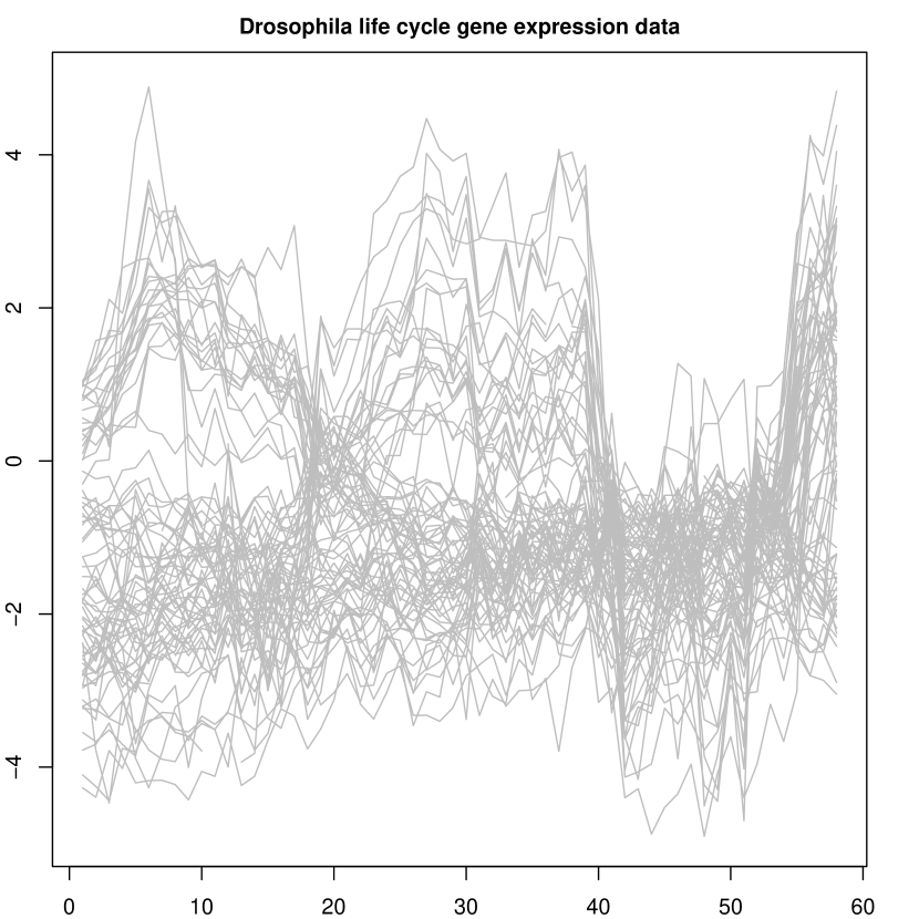
Figure 1: Subset of the drosophila melanogaster life cycle gene expression data.

Even if hardly identifiable by eyes, in Figure 1, three classes of genes can be distinguished according to their gene expressions (see Section 5). Our interest here is to introduce a strategy to automatically partition these objects (time series) in homogeneous groups. This kind of problem is often solved by defining a suitable “clustering procedure”. In the last years many techniques have been proposed to define homogeneous groups in time series data. A rich overview can be found in Liao (2005).

One of the first references on this topic is Maharaj (2000) that proposed a two stage approach based on the hypothesis that the observed series could be modeled by invertible and stationary ARMA processes. A different point of view has been adopted by Baragona (2001) which suggested a series of meta-heuristic approaches (e.g. simulated annealing, tabu search and the genetic algorithms) to partition stationary time series according the cross-correlations estimated from the residuals of models estimated on the original data. Self organizing map (SOM) algorithms have began popular clustering tools. An example of their application in longitudinal data analyzes is the method of Fu et al. (2001).

Kumar et al. (2002) worked in a different direction and studied a new scale-invariant distance function based on the hypothesis of Gaussian distributed errors. In their model, time series sampled at $T$ points are represented by a sequence of probability distributions assumed independent and identically normally distributed. Möller-Levet et al. (2003) introduced a short time series distance in order to measure the similarity between different series by measuring the relative change in the signal amplitudes.

Within a Bayesian framework, Ramoni et al. (2002) suggested to cluster univariate series by recursively merging the ones showing similar dynamics. In order to summarize a dynamic process by a transition probability matrix, each series is converted into a Markov Chain (MC) on which a clustering algorithm is then performed. This approach, known as Bayesian clustering by dynamics (BCD), adopts the posterior probability scoring metric to define the possible partitions searching for the one with the highest posterior probability through an entropy-based method.

Many of the algorithms mentioned above do not facilitate the removal of the noise from data, encounter difficulties in handling data with missing values, require some pre-process of the series and do not account for possible correlation in the measurement errors. Furthermore, when a large number of observations is considered, the computational effort related to the clustering task can become prohibitive. In order to overcome these hitches, many authors have suggested to exploit a flexible definition of the series functional form and to adopt some dimensionality reduction strategy. To these class belong the proposals based on the functional data analysis framework (Ramsay and Silverman, 2005). The main idea is to describe the data by using optimal linear combinations of basis functions (e.g. by using B-spline bases) and to perform the clustering on the extracted signals or on the estimated basis coefficients (when possible).

An example is the proposal of Chiou and Li (2007) exploiting a functional principal analysis of the raw series. Sangalli et al. (2010) suggested a functional k-means method to partition misaligned data series. James and Sugar (2003) introduced the fclust approach. Within this framework, the raw data are modeled by linear combinations of spline bases. The regression spline coefficients are clustered taking them as distributed according to a mixture of Gaussian distributions with cluster specific means and common variance-covariance matrix. The spline bases are defined over equally spaced knots and their optimal number is chosen through cross-validation. A similar regression spline based approach has been proposed by Abraham et al. (2003) in combination with a k-means clustering procedure.

In a similar direction moves the work of Coffey et al. (2014). The authors suggest to model the raw series by using truncated power P-spline smoothers Ruppert et al. (2003). They exploit the connection between P-splines and linear mixed models to define a suitable variance-covariance cluster matrix to be used in a Gaussian mixture model. Within the Bayesian settings, a similar point of view has been adopted by Komárek and Komárková (2013) for clustering continuous and discrete longitudinal data.

In this paper we propose a parsimonious model-based approach for clustering longitudinal data. In particular we model the raw series by a linear combination of B-spline which coefficient are shrunk by difference penalties. This is the P-spline smoothing approach introduced by Eilers and Marx (1996). We model each series by P-splines and perform a cluster analysis on the optimal spline coefficients. This idea can be potentially adopted within many of the most popular clustering methods but, in the present work, we focus our attention on the k-means one.

Our framework differs from the ones of James and Sugar (2003), Abraham et al. (2003) and Coffey et al. (2014) due to the choice of the smoother. Indeed, B-spline based P-spline smoothers allow for a valuable simplification of the partitioning process. As discussed in Eilers and Marx (2010) the P-spline coefficients represent the skeleton of the final fit. By summarizing the raw data using the estimated spline coefficients, one obtains an efficient reduction of the dimensionality of the partitioning task. This is not true if truncated bases P-splines are adopted (as in Coffey et al. (2014)). In addition, by shrinking the spline coefficients through difference penalties, the shape of the final smoothing function becomes quite insensitive to the choice of the number of bases and to their position allowing for efficient data interpolation in the case missing values (this is an advantage with respect to the proposals of James and Sugar (2003) and Abraham et al. (2003)).

This paper is organized as follows. Section 2 reviews the P-splines smoothing framework discussing briefly the main features that will be useful for our applications. In section 3 we introduce our proposal within the k-means clustering framework. In Section 4 the performances of our method are evaluated through simulation while in Section 5 the gene expression data of Figure 1 are analyzed. Section 6 concludes the paper with a discussion on our achievements and possible future research guidelines.

2 P-splines in a nutshell

P-splines have been introduced by Eilers and Marx (1996) as flexible smoothing procedures combining B-spline bases (see e.g. de Boor, 1978) and difference penalties.

Suppose to observe a set of data $\{x,y\}_{j=1}^{n_{i}}$ where the vector $\boldsymbol{x}$ indicates the independent variable (e.g. time) and ${\boldsymbol{y}}$ the dependent one. Our aim is to describe the available measurements through an appropriate smooth function. We assume that the observed series can be modeled as:

$$\boldsymbol{y}=f(\boldsymbol{x})+{\boldsymbol{\epsilon}},$$ (2.1)

where $\boldsymbol{\epsilon}$ is a vector of errors and $f(\cdot)$ is an unknown smooth function.

Denote with $\boldsymbol{B}_{h}(x;q)$ the value of the $h$th B-spline of degree $q$ defined over a domain spanned by $m$ equidistant knots (in what follows we consider always equally spaced knots as suggested by Eilers and Marx (1996, 2010)). A curve that fits the data is given by $\hat{y}(x)=\sum_{h}a_{h}\boldsymbol{B}_{h}(x;q)$ where $a_{h}$ (with $h=1,...,m+q$) are the B-splines coefficients estimated through least squares. Unfortunately the curve obtained by minimizing $\|{\boldsymbol{y}}-{\boldsymbol{B}\boldsymbol{a}}\|^{2}$ w.r.t. $\boldsymbol{a}$ shows more variation than is justified by the data if a dense set of spline functions is used. In order to avoid overfitting one can estimate ${\boldsymbol{a}}$ in a penalized regression setting:

$$\hat{{\boldsymbol{a}}}=\mathop{\mbox{argmin}}_{{\boldsymbol{a}}}\|{\boldsymbol{y}}-{\boldsymbol{B}\boldsymbol{a}}\|^{2}+\lambda\|{\boldsymbol{D}_{d}\boldsymbol{a}}\|^{2},$$ (2.2)

where $\boldsymbol{D}_{d}$ is a $d$th order difference penalty matrix such that ${\boldsymbol{D}_{d}\boldsymbol{a}}=\Delta^{d}{\boldsymbol{a}}$ defines a vector of $d$th order differences of the coefficients. Usually $d=2$ or $d=3$ is used. A second order difference matrix appears as follows:

$${\boldsymbol{D}}_{2}=\left[\begin{array}[]{cccccc}1&-2&1&\cdots&0&0\\ 0&1&-2&1&\cdots&0\\ \vdots&\ddots&\ddots&\ddots&\ddots&\vdots\\ 0&0&\cdots&1&-2&1\\ \end{array}\right].$$

The optimal spline coefficients follow from (2.2) as:

$$\hat{{\boldsymbol{a}}}=({\boldsymbol{B}}^{\top}{\boldsymbol{B}}+\lambda{\boldsymbol{D}}^{\top}{\boldsymbol{D}})^{-1}{\boldsymbol{B}}^{\top}{\boldsymbol{y}}.$$ (2.3)

The (positive) parameter $\lambda$ controls the degree of smoothness of the final fit. For a smoothing parameter close to zero the final smoother tends to interpolate the observations (leading to overfitting) while, for large values of $\lambda$, the fitted function will tend to a polynomial of degree $d-1$.

Figure 2 shows the estimated P-splines for different values of the smoothing parameters (for brevity only four $\lambda$ values are considered). The data have been simulated by adding a Gaussian noise to a sinusoidal signal (50 observations). Large portions of observations have been omitted to simulate the presence of missing values. Cubic B-splines defined on 30 equidistant knots and third order penalties have been used.

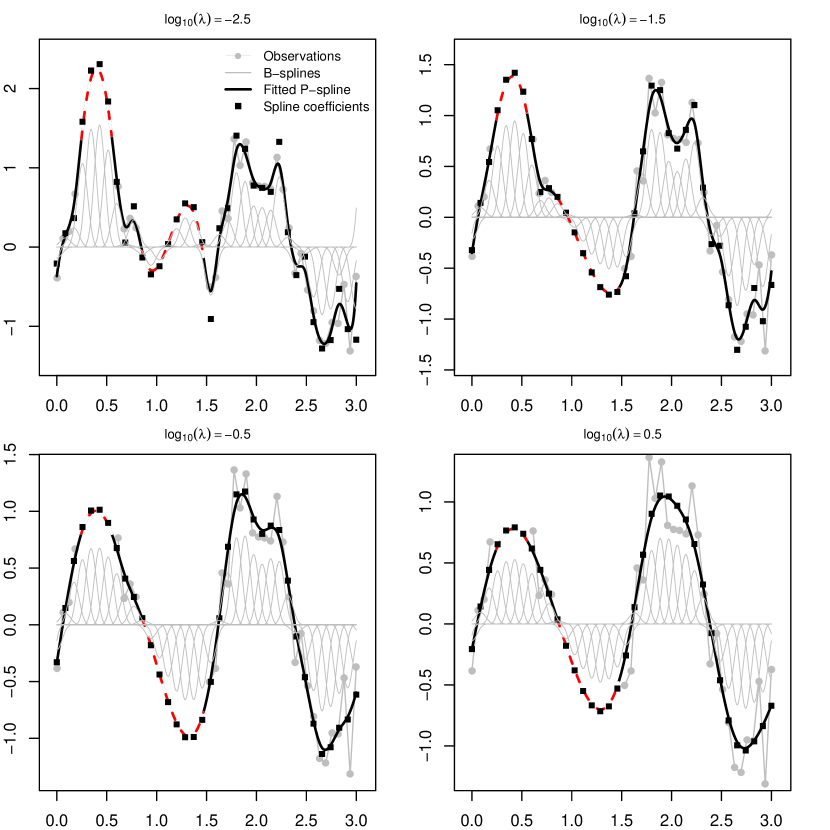
Figure 2: Smoothing and interpolation with P-splines (solid black lines) for different values of the $\lambda$ parameters (in a $\log_{10}$ scale). The dashed red segments represent the estimated signals in correspondence of missing data. The squared dots indicate the estimated optimal spline coefficients. The scaled basis functions are shown at the bottom of each graph.

As it appears form Figure 2, the spline coefficients (squared dots) represent the skeleton of the fitted smoother. It can be shown that the coefficients of interpolating P-splines define a polynomial sequence of degree $2d-1$ and that, thanks to the penalty, they are forced to follow a smooth pattern also when some observations are missed.

The selection of the optimal number of basis functions and their location are crucial in spline regression applications and greatly influence the final fit. P-splines make these choices not particularly relevant. Indeed, the shape of the final smoother is mostly governed by the smoothing parameter and is hardly influenced by the richness of the basis matrix and by the knot location. This is due to the characteristics of the penalty and of the basis functions. Figure 3 investigates this aspect where the optimal smoothing parameters have been selected through the V-curve procedure introduced in Section 2.1. For this reason, we perform all our analyzes using smoothers built over a generous number of equally spaced knots (but still smaller than the available observations).

For a complete discussion about the properties of the P-spline smoother we refer to Eilers and Marx (1996, 2010). These features are not shared by other definitions of P-splines (e.g. the truncated power P-splines exploited by Coffey et al. (2014)) and by regression splines (suggested by Abraham et al. (2003) and James and Sugar (2003) for functional clustering applications) and play a crucial role in the method described in this paper.

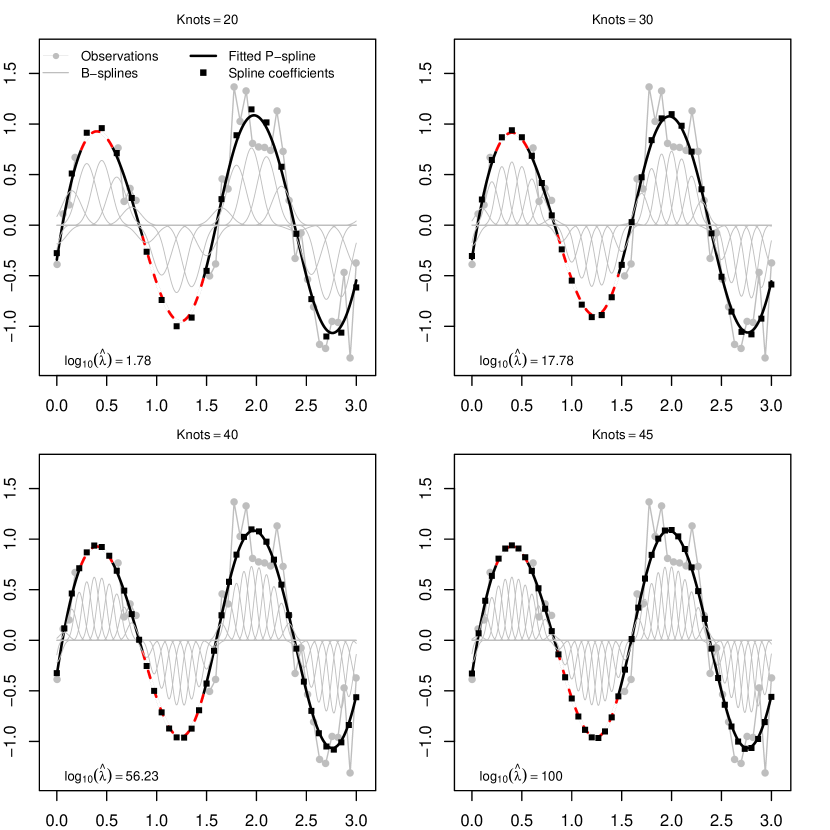
Figure 3: Smoothing and interpolation with P-splines (solid black lines) for different numbers of B-spline bases defined on equally spaced knots. The value of the optimal smoothing parameters have been selected using the V-curve criterion. The dashed red segments represents the estimated signals in correspondence of missing data. The squared dots indicates the estimated optimal spline coefficients. The scaled basis functions are shown at the bottom of each graph.

2.1 Smoothing parameter selection

From Figure 2 it clearly appears that the shape of the fitted functions depends on the value of the smoothing parameter. For this reason it is of great interest to select the optimal $\lambda$ by a reliable automatic procedure. The Akaike information criterion, the Bayesian information criterion and the (generalized) cross validation are popular alternatives.

These “classical” methods suffer of two drawbacks: 1) they require the computation of the effective model dimension (see e.g. Hastie and Tibshirani (1990)) which can become time consuming for a rich set of B-spline functions, and 2) they are sensitive to serial correlation in the noise around the trend (leading to overfitting). This last aspect is crucial in many applications. For this reason, in all the examples presented in this paper, we have adopted the V-curve criterion to select the optimal smoothing parameter.

The V-curve can be viewed as a convenient simplification of the L-curve framework proposed by Hansen (1992). The L-curve is a parameterized curve comparing the two ingredients of every regularization or smoothing procedure: badness of the fit and roughness of the final estimates. Given a P-spline defined for a fixed $\lambda$, the following quantities can be computed:

$$\{\omega(\lambda);\theta(\lambda)\}=\{\|{\boldsymbol{y}}-{\boldsymbol{B}}\hat{{\boldsymbol{a}}}(\lambda)\|^{2};\|{\boldsymbol{D}}\hat{{\boldsymbol{a}}}(\lambda)\|^{2}\}.$$

The L-curve is the plot of $\psi(\lambda)=\log(\omega)$ against $\phi(\lambda)=\log(\theta)$ evaluated over a grid of smoothing parameters. This plot typically shows a L-shaped curve and the optimal amount of smoothing is located in the corner of the “L” by maximizing a measure of the local curvature.

The V-curve criterion simplifies this selection criterion by requiring the minimization of the Euclidean distance between the adjacent points lying on the L-curve. The optimal smoothing parameter is then the one minimizing $V(\lambda)=\sqrt{\{\Delta\psi(\lambda)\}^{2}+\{\Delta\phi(\lambda)\}^{2}}$ ($\Delta$ indicates the first order difference operator). In this way the computation of the partial second derivatives needed for the evaluation of the local curvature is avoided (see Frasso and Eilers (2015) for a detailed discussion).

3 P-spline based k-means procedure

Any cluster analysis requires two choice: the identification of a suitable clustering algorithm and the selection of an appropriate distance measure. In what follows, we introduce the notations, the clustering algorithm and the distance measures used in the paper.

3.1 Notations and definitions

Let $\boldsymbol{y}_{i}$ be the ${i}$th observed series with $i=1,\ldots,N$. Let $\boldsymbol{c}_{k}$ be the $k$th cluster center, with $k=1,\ldots,K$ and $1<K<N$. Define as $\boldsymbol{a}_{i}$ the $[(m+q)\times 1]$ vector of optimal spline coefficients estimated for the $i$th series. Finally, in what follows, we indicate with $x_{j}$, $j=1,\ldots,n_{i}$, the time points over which the $i$th series is observed.

3.2 Clustering algorithm and distance measures

The k-means algorithm (see e.g. MacQueen (1967) and Hartigan and Wong (1979)) is one of the most popular clustering approaches. It relies on an iterative scheme. The procedure aims to partition the observations in a predetermined number ($K$) of clusters. In the case the algorithm is applied to the P-spline coefficients estimated for $N$ time series, its steps can be summarized as follows:

• Initialization: fit a P-spline smoother to each series and store the optimal spline coefficient in a matrix $\boldsymbol{A}=[\widehat{a}_{i,h}]$ of dimension $[(m+q)\times N]$. Assign randomly the columns of $\boldsymbol{A}$ to $K$ groups representing the initial clusters.

• Assign each sequence $\boldsymbol{a}_{i}$ to the cluster whose distance from the center is minimum.

• When all objects have been assigned to a group, update the positions of the $K$ cluster centroids.

The procedure is stopped when the cluster centers do not move any more. Otherwise steps 2 and 3 are repeated until convergence.

The $K$ centroids $({\boldsymbol{c}_{k}|k=1,...,K})$ are defined as the minimizers of:

$$J=\sum_{i=1}^{N}\sum_{k=1}^{K}\mathcal{D}(\boldsymbol{a}_{i},\boldsymbol{c}_{k})$$ (3.1)

where $\mathcal{D}(\boldsymbol{a}_{i},\boldsymbol{c}_{k})$ is a distance (dissimilarity) measure between the $i$th spline coefficient vector and the $k$th cluster center. In what follows we focus on two distances: the Euclidean distance and the distance based on the Pearson’s correlation coefficient.

The Euclidean distance is computed as follows:

$$\mathcal{D}_{2}=\sum_{i=1}^{N}\sum_{k=1}^{K}\|\boldsymbol{a}_{i}-\boldsymbol{c}_{k}\|^{2}$$ (3.2)

In time series applications, a distance measure based on the Pearson’s correlation coefficient is often a valid alternative to (3.2):

$$\mathcal{D}_{\rho}=1-\rho(\boldsymbol{a}_{i},\boldsymbol{c}_{k}),$$ (3.3)

where $\rho(\cdot)$ is the Pearson’s correlation coefficient.

The mentioned metrics are defined in the time domain. Distances defined in the frequency domain can be more appropriate to measure the similarity between time series in particular applications. We refer to Vilar et al. (2010) and Montero and Vilar (2014) for a detailed discussion about possible distance measures applicable in time series clustering tasks.

Finally notice that, in the case of normally distributed errors in Eq. 2.1, the asymptotic properties of the k-means algorithm described above can be proven following the lines discussed in Abraham et al. (2003).

4 Simulations

In order to test the performances of our proposal we present here the results of a simulation study.

We have generated $K=6$ clusters of series observed over $100$ time points with $x_{j}\in[0,1]$. Each cluster is formed by adding an error term to a specific signal functional form. We defined the following functional classes:

Sin $$y_{ij}^{(1)}=\alpha_{i}\sin(4\pi x_{ij})+\beta_{i}+\epsilon_{ij}$$

Cubic $$y_{ij}^{(2)}=\alpha_{i}(x_{ij}+0.73)^{3}+\beta_{i}+\epsilon_{ij}$$

Neg-pow $$y_{ij}^{(3)}=\alpha_{i}(x_{ij}+0.5)^{-3/2}+\beta_{i}+\epsilon_{ij}$$

Cos $$y_{ij}^{(4)}=\alpha_{i}\cos(2\pi x_{ij})+\beta_{i}+\epsilon_{ij}$$

Exp $$y_{ij}^{(5)}=\alpha_{i}\exp(-6x_{ij})+\beta_{i}+\epsilon_{ij}$$

Lin $$y_{ij}^{(6)}=-\alpha_{i}(x_{ij}-0.5)+\beta_{i}+\epsilon_{ij},$$

where $\alpha_{i}\sim{\cal N}(4,\sigma^{2}_{\alpha})$ and $\beta_{i}\sim{\cal N}(0,\sigma^{2}_{\beta})$ with $\sigma_{\alpha}$ and $\sigma_{\beta}$ drawn from ${\cal U}(0.3,1)$.

We have taken into account three possible scenarios for the error component $\boldsymbol{\epsilon}_{i}$: scenario 1) a zero mean normally distributed noise with standard deviation $\sigma_{\epsilon}\sim{\cal U}(0,0.5)$; scenario 2) a first order autoregressive model with $\sigma_{\epsilon}\sim{\cal U}(0,0.5)$ and correlation coefficient $\rho=0.5$; scenario 3) a similar autoregressive process with $\rho=0.9$.

For each class have been generated respectively 90, 50, 100, 25, 60 and 35 series. Each series have been modeled by P-splines taking cubic bases and third-order penalties. The optimal smoothing parameters have been selected through a V-curve procedure (introduced in Section 2).

Moreover, we have considered both complete and incomplete observations. In the latter case, the missing mechanism has been simulated by excluding independently and uniformly some observations from each series. The percentage of missing values for each series has been supposed uniformly distributed between 10% and 50%. Figure 5 and Figure 5 show some simulated datasets.

Figure 4: Example of simulated data without missing observations.

Figure 5: Example of simulated data with missing observations.

For this simulation study we used a k-means algorithm based on the Pearson’s correlation distance. The procedure was run taking 50 random starting point with 50 replicates. To check the sensitivity of our procedure with respect to a different number of cubic splines, we performed the analyzes by taking the number of internal knots equal to the 10%, 20%, 30%, 40% of the observations. In order to evaluate the clustering performances we computed the Adjusted Rand Index (ARI) validation criterion (Hubert and Arabie, 1985). The results have been obtained over 100 replicates per each scenario.

We compare the performances of the proposed approach with those achieved by two frameworks based on the k-means partitioning: one exploiting regression splines (see e.g. Abraham et al., 2003) and the functional PCA k-means approach of Chiou and Li (2007).

4.1 Simulation results with complete observations

Figure 6 shows the box-plots of the ARI values for the P-splines based k-means approach (left column) and for a k-means clustering based on regression splines coefficients (right column). In both cases we have used cubic B-splines defined over equally spaced knots. The performances have been evaluated considering complete observations. In each cell of the figure matrix four box-plots are shown according to the different number of spline functions involved in the smoothing procedure.

The clustering performances of the P-spline based k-means method seem quite insensitive to the choice of the number of internal knots. Even with cubic B-splines defined over 10 equally spaced interior knots, the mean ARI was found equal to $0.98$, $0.96$ and $0.94$ for scenario 1, 2 and 3, respectively. As expected, the variability of the ARI distributions seems to be influenced by the number of knots used to build the P-splines smoothers (especially for relatively small number of spline functions). Finally, regardless the correlation of the error component, the mean ARI values grow (slightly) with the number of internal knots even if it was found close to $1$ for all the settings.

The regression spline based procedure shows a lower classification quality in all the simulation settings. This can be explained by the fact that, without the introduction of a smoothing penalty, the estimated spline coefficients (and then the final fits) are strongly influenced by the number and the position of the knots used to define the basis functions. These aspects are not crucial for P-spline smoothers as discussed in Section 2.

As expected, the computational cost of the two procedures tends to be larger as the number of bases increases. Nevertheless, for the P-spline based classification, the average times required by using cubic B-splines defined over 10 equally spaced interior knots was found equal to $2.5$, $2.8$ and $3$ seconds for scenario 1, 2 and 3, respectively and increases (approximately) proportionally with the number of spline knots. The computational burden for the k-means partitioning based on regression spline coefficients is significantly lower given that the selection of the smoothing parameter is not required.

These results can be compared with the one achieved by the functional PCA k-means approach proposed by Chiou and Li (2007) (upper panel of Figure 8). This approach ensures performances close to the ones registered by the P-spline based k-means and appears robust to the characteristics of the error terms.

Figure 6: Clustering results for simulated series with complete observations. The panels on the left column present the box-plots of the ARI values registered for the P-spline based approach for different numbers of spline functions and different definitions of the noise term. The results obtained by using a k-means partitioning of the regression spline coefficients are shown in the right column.

4.2 Simulation results with missing observations

Figure 7 shows the performances of the P-splines based k-means approach (left column) and of the k-means clustering procedure based on regression splines coefficients (right column) in presence of missing observations. The box-plots in each panel summarize the distribution of the ARI values computed for different number of spline functions.

For the P-spline based k-means procedure, the average ARI values were found lower than the ones obtained for the complete observation case but still above above 95% for all the simulation settings. On the other hand, the presence of missing observations have a strong impact on the performances of the regression spline k-means method. This difference between the two approaches can be easily explained by considering the interpolation properties guaranteed by the finite difference penalty matrix involved in the definition of the P-spline smoothers.

As expected also in this case an increasing number of knots requires a larger computational effort, whatever the scenario for the error component. For the P-spline based k-means procedure, the average time required by using 40 equally spaced interior knots was equal to $7.07$, $7.08$ and $7.5$ seconds for scenario 1, 2 and 3, respectively.

Finally, these results can be compared with those achieved by the functional PCA k-means approach (lower panel of Figure 8). As before, this method ensures performances closer to the ones registered for the P-spline based k-means framework.

Figure 7: Clustering results for simulated series with missing observations. The panels on the left column present the box-plots of the ARI values registered for the P-spline based approach for different numbers of spline functions and different definitions of the noise term. The results obtained by using a k-means partitioning of the regression spline coefficients are shown in the right column.

Figure 8: Clustering performances of the functional PCA k-means approach. The upper panel shows the distribution of the ARI values registered for complete datasets while the lover plot indicates the ones observed for datasets with missing observations.

5 Clustering drosophila gene expression data

In this section we analyze the data introduced in Section 1. As already mentioned, Arbeitman et al. (2002) have identified three gene categories according to their biological functions. In the data of Figure 1, it is possible to identify $23$ muscle-specific, $33$ eye-specific and $21$ transient early zygotic genes (upper left panel of Figure 9). Our aim here is to test the capability of the P-spline based k-means procedure introduced above in identifying these groups.

In order to partition the data we used a k-means algorithm based on the Euclidean distance. We set $K=3$ possible clusters. The analysis has been performed by taking $100$ replicates of the partitioning procedures in order to avoid local minima. Each gene expression profile has been smoothed by P-splines. We used third order penalties and cubic B-splines defined over 25 equally spaced interior knots.

Figure 9 shows the results of our clustering proposal. The recognized center are really similar to the “true” ones defined in Arbeitman et al. (2002).

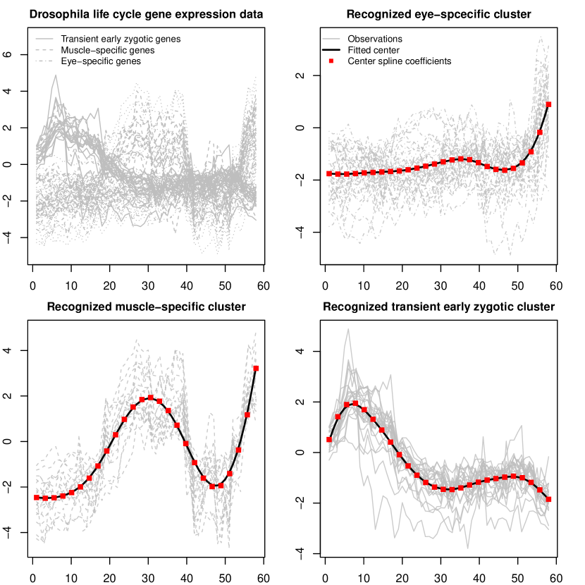
Figure 9: Gene expression profiles clustered by k-means procedure with Euclidean distance. For each subplot the horizontal axis represents the time and the vertical axis the gene expression level. The gray lines reproduce the raw data series assigned to each cluster. The red dots indicate the estimated optimal spline coefficients for cluster center. The black solid lines indicate the center functionals.

The entire analysis has been performed in less than a second. The adjusted rand index, computed on the basis of the groups identified by Arbeitman et al. (2002), was found approximately equal to $0.96$. The goodness of our results can also be appreciated by looking at the homogeneity of the functions assigned to each cluster. Furthermore, these results are consistent with those presented by Chiou and Li (2007).

In this application, as in the simulation exercise presented above, we did not select the optimal number of clusters taking it as known. However, all the cluster selection procedures proposed in the literature for k-means partitioning are in principle applicable to the discussed method.

6 Discussion

In this paper we have presented a parsimonious clustering method suitable for time series applications. The idea behind our proposal is quite simple but efficient. We suggest to model each series by P-spline smoothers as defined by Eilers and Marx (1996) and to perform a cluster analysis on the estimated coefficients. This makes possible to summarize the observed series in a lower-dimensional vector of parameters.

As briefly discusses in Section 2, P-splines show a series of desirable properties that make the introduced procedure particularly attractive (a detailed discussion is presented by Eilers and Marx (2010)). First of all, the optimal P-spline coefficients are close to the fitted curve and represent the skeleton of the final fit. Second, the final estimates are hardly influenced by the number and location of the knots used to define the B-spline bases and depend mainly on the weight assigned to the roughness penalty. Finally, the combination of B-spline functions and difference penalty ensure an efficient interpolation of the observed measurements also when some of them are missed.

In order to select the optimal amount of smoothing to apply to each series we suggested to use a V-curve approach. Even if alternative criteria (such as AIC, BIC and cross validation) can be adopted, the V-curve appears particularly appealing from a computational point of view and ensures robustness against possible correlation in the noise of the observed data (we refer to Frasso and Eilers (2015) for a complete discussion about these aspects).

In this work we have chosen to classify the estimated spline coefficients by k-means algorithm. The performance of our P-spline based k-means approach have been evaluated by intensive simulations. Our simulation study has shown that, both in presence of complete or missing observations, our proposal ensures high quality performances in a reasonable computational time regardless the complexity (in terms of number of spline functions) of the adopted P-spline models. Furthermore, the comparison with the functional k-means settings introduced by Abraham et al. (2003) and Chiou and Li (2007) indicates our methodology as an attractive alternative.

In Section 5 we used our approach to analyze a set of drosophila melanogaster gene expression data. Our results appear particularly encouraging since the adjusted rand index (ARI), computed according to the classification of Arbeitman et al. (2002), has been found approximately equal to 0.96. Moreover, our results are consistent with those obtained by Chiou and Li (2007) for the same dataset.

Some aspects have not been investigated yet and will guide our further research. First, we believe that our proposal can be valuable also within clustering frameworks different from the k-means one. Second, in all the examples proposed here, we supposed a smooth signal describing the trend of the series. In some cases, for example by dealing with EEG or spectroscopy measurements, this hypothesis does not appear appropriate and different definitions of the P-spline penalty could be useful. Finally, P-splines are easily generalizable to analyze discrete observations and multidimensional (e.g. defined over space and time) measurements (see e.g. Marx and Eilers, 2005; Eilers and Marx, 1996, 2010). We have intention to investigate the possibility to extend the P-spline based k-means procedure in order to deal with such data.

References

- Abraham et al. (2003) Abraham, C., Cornillon, P. A., Matzner-Løber, E., and Molinari, N. (2003). Unsupervised curve clustering using b-splines. Scandinavian Journal of Statistics, 30(3), 581–595.
- Arbeitman et al. (2002) Arbeitman, M. N., Furlong, E. E. M., Imam, F., Johnson, E., Null, B. H., Baker, B. S., Krasnow, M. A., Scott, M. P., Davis, R. W., and White, K. P. (2002). Gene expression during the life cycle of drosophila melanogaster. Science, 297(5590), 2270–2275.
- Baragona (2001) Baragona, R. (2001). A simulation study on clustering time series with meta-heuristic methods. Quaderni di Statistica, 3, 1–26.
- Chiou and Li (2007) Chiou, J.-M. and Li, P.-L. (2007). Functional clustering and identifying substructures of longitudinal data. Journal of the Royal Statistical Society: Series B (Statistical Methodology), 69(4), 679–699.
- Coffey et al. (2014) Coffey, N., Hinde, J., and Holian, E. (2014). Clustering longitudinal profiles using p-splines and mixed effects models applied to time-course gene expression data. Comput. Stat. Data Anal., 71, 14–29.
- de Boor (1978) de Boor, C. (1978). A Practical Guide to Splines. Applied Mathematical Sciences. Springer New York.
- Eilers and Marx (1996) Eilers, P. H. C. and Marx, B. D. (1996). Flexible smoothing with b-splines and penalties. Statistical Science, 11, 89–121.
- Eilers and Marx (2010) Eilers, P. H. C. and Marx, B. D. (2010). Splines, knots, and penalties. Wiley Interdisciplinary Reviews: Computational Statistics, 2(6), 637–653.
- Frasso and Eilers (2015) Frasso, G. and Eilers, P. H. (2015). L- and v-curves for optimal smoothing. Statistical Modelling, 15(1), 91–111.
- Fu et al. (2001) Fu, T.-c., Chung, F.-l., Ng, V., and Luk, R. (2001). Pattern discovery from stock time series using self-organizing maps. Workshop Notes of KDD2001 Workshop on Temporal Data Mining, pages 26–29.
- Hansen (1992) Hansen, P. C. (1992). Analysis of Discrete Ill-Posed Problems by Means of the L-curve. SIAM Review, 34(4), pp. 561–580.
- Hartigan and Wong (1979) Hartigan, J. and Wong, M. (1979). Algorithm AS 136: A K-means clustering algorithm. Applied Statistics, pages 100–108.
- Hastie and Tibshirani (1990) Hastie, T. J. and Tibshirani, R. J. (1990). Generalized additive models. London: Chapman & Hall.
- Hubert and Arabie (1985) Hubert, L. and Arabie, P. (1985). Comparing partitions. Journal of Classification, 2(1), 193–218.
- James and Sugar (2003) James, G. M. and Sugar, C. A. (2003). Clustering for sparsely sampled functional data. Journal of the American Statistical Association, 98, 397–408.
- Komárek and Komárková (2013) Komárek, A. and Komárková, L. (2013). Clustering for multivariate continuous and discrete longitudinal data. Ann. Appl. Stat., 7(1), 177–200.
- Kumar et al. (2002) Kumar, M., Patel, N. R., and Woo, J. (2002). Clustering seasonality patterns in the presence of errors. In Proceedings of the Eighth ACM SIGKDD International Conference on Knowledge Discovery and Data Mining, KDD ’02, pages 557–563.
- Liao (2005) Liao, W. T. (2005). Clustering of time series data-a survey. Pattern Recogn., 38(11), 1857–1874.
- MacQueen (1967) MacQueen, J. (1967). Some methods for classification and analysis of multivariate observations. In L. M. Le Cam and J. Neyman, editors, Proceedings of the 5th Berkeley Symposium on Mathematical Statistics and Probability - Vol. 1, pages 281–297. University of California Press, Berkeley, CA, USA.
- Maharaj (2000) Maharaj, E. (2000). Cluster of time series. Journal of Classification, 17(2), 297–314.
- Marx and Eilers (2005) Marx, B. D. and Eilers, P. H. (2005). Multidimensional penalized signal regression. Technometrics, 47(1), 13–22.
- Möller-Levet et al. (2003) Möller-Levet, C., Klawonn, F., Cho, K.-H., and Wolkenhauer, O. (2003). Fuzzy clustering of short time-series and unevenly distributed sampling points. In Advances in Intelligent Data Analysis V, volume 2810, pages 330–340. Springer Berlin Heidelberg.
- Montero and Vilar (2014) Montero, P. and Vilar, J. A. (2014). Tsclust: An r package for time series clustering. Journal of Statistical Software, 62(1), 1–43.
- Ramoni et al. (2002) Ramoni, M., Sebastiani, P., and Cohen, P. (2002). Bayesian clustering by dynamics. Machine Learning, 47(1), 91–121.
- Ramsay and Silverman (2005) Ramsay, J. O. and Silverman, B. W. (2005). Functional Data Analysis. Springer Series in Statistics. Springer, 2nd edition.
- Ruppert et al. (2003) Ruppert, D., Wand, P., and Carroll, R. (2003). Semiparametric Regression. Cambridge Series in Statistical and Probabilistic Mathematics. Cambridge University Press.
- Sangalli et al. (2010) Sangalli, L. M., Secchi, P., Vantini, S., and Vitelli, V. (2010). K-mean alignment for curve clustering. Computational Statistics & Data Analysis, 54(5), 1219 – 1233.
- Vilar et al. (2010) Vilar, J. A., Alonso, A. M., and Vilar, J. M. (2010). Non-linear time series clustering based on non-parametric forecast densities. Computational Statistics & Data Analysis, 54(11), 2850–2865.