Astrophysical S factor of ¹²C($\alpha,\gamma$)¹⁶O Calculated with the Reduced R-matrix Theory

Abstract

Determination of the accurate astrophysical S factor of ¹²C($\alpha,\gamma$)¹⁶O reaction has been regarded as a holy grail of nuclear astrophysics for decades. In current stellar models, a knowledge of that value to better than 10% is desirable. Due to the practical issues, tremendous experimental and theoretical efforts over nearly 50 years are not able to reach this goal, and the published values contradicted with each other strongly and their uncertainties are 2 times larger than the required precision. To this end we have developed a Reduced R-matrix Theory, based on the classical R-matrix theory of Lane and Thomas, which treats primary transitions to ground state and four bound states as the independent reaction channels in the channel spin representation. With the coordination of covariance statistics and error propagation theory, a global fitting for almost all available experimental data of ¹⁶O system has been multi-iteratively analyzed by our powerful code. A reliable, accurate and self-consistent astrophysical S factor of ¹²C($\alpha,\gamma$)¹⁶O was obtained with a recommended value $S_{tot}$ (300) = 162.7 $\pm$ 7.3 keV b (4.5%) which could meet the required precision.

I Introduction

During core-He burning 3$\alpha$ and ¹²C($\alpha,\gamma$)¹⁶O reactions compete to determine the helium burning time scale, together with the convection mechanism, and the relative abundances of oxygen and carbon prior to core-C burning. W. A. Fowler, a Nobel laureate in physics in 1983, definitely held a view that the abundance ratio of ¹²C to ¹⁶O and the solar neutrino problem are serious difficulties in the most basic concepts of nuclear astrophysics Rolf88 . The work of many investigators has resulted in a knowledge of the predicted reaction rate of 3$\alpha$ process within about 10% Fynb05 accuracy at the usual helium-burning temperatures. Unfortunately, the same of the ¹²C($\alpha,\gamma$)¹⁶O reaction is much less well determined, and it is highly desirable to know this rate with comparable accuracy Woos07 to that of the 3$\alpha$ process in order to provide adequate constraints on stellar evolution and the synthesis of elements, e.g. the yield of the neutrino-process isotopes ⁷Li, ¹¹B, ¹⁹F, ¹³⁸La and ¹⁸⁰Ta in core-collapse supernovae Aust11 ; Aust14 , and the production of the important radioactive nuclei ²⁶Al, ⁴⁴Ti, and ⁶⁰Fe Tur10 .

Table 1: Comparison of the astrophysical S factor (keV b) at 0.3 MeV obtained in various fits, including this work, for the E10, E20, cascade transitions components, as well as the total.

$Reference$	$S_{tot}$	$S_{E10}$	$S_{E20}$	$S_{cas}$
This work	162.7$\pm$7.3	98.0$\pm$7.0	56.0$\pm$4.1	8.7$\pm$1.8
Schürmann Schu12	161$\pm$19	83.4	73.4	4.4
Oulebsir Oule12	175$\pm$63	100$\pm$28	50$\pm$19	—
Sayre Sayr12	—	—	$62_{-6}^{+9}$	—
Tang Tang10	—	84$\pm$21	—	—
Matei Mate08	—	—	—	$S_{6.92}$=7.0$\pm$1.6
Matei Mate06	—	—	—	$S_{6.05}$=$25_{-16}^{+25}$
Hammer Hamm05	162$\pm$39	77$\pm$17	80$\pm$20	4$\pm$4
Tischhauser Tisc02	149$\pm$29	80$\pm$20	$53_{-18}^{+13}$	16$\pm$16
Kunz Kunz01	165$\pm$50	76$\pm$20	85$\pm$30	4$\pm$4
Brune Brun99	159	101$\pm$17	$42_{-23}^{+16}$	16
Ouellet Ouel96	120$\pm$40	79$\pm$16	36$\pm$6	—
Buchmann Buch96	165$\pm$75	79$\pm$21	70$\pm$70	16$\pm$16

The most direct and trustworthy way to obtain the astrophysical S factor of the ¹²C($\alpha,\gamma$)¹⁶O reaction is to measure the cross section for that reaction till as low energy as possible, and to extrapolate to energies of astrophysical interest. The astrophysical S factor for ¹²C($\alpha,\gamma$)¹⁶O reaction reaction is given by

$$S(E)=\sigma(E)\cdot E\cdot\exp(2\pi\eta),$$ (1)

where $\eta$ = $Z_{\alpha}Z_{C}e^{2}/\hbar\nu$ is the Sommerfeld parameter for the interaction particles. To investigate the specific role of the ¹⁶O nucleus for the S factor, a wealth of experimental data have been accumulated over the past few decades, including the precise measurements of total cross-section of ¹²C($\alpha,\gamma$)¹⁶O Schu05 ; Schu11 ; Plag12 ; Fuji13 , $\gamma$-ray angular distributions of ground state transition Dyer74 ; Redd87 ; Ouel96 ; Kunz97 ; Kunz01 ; Assu06 ; Fey04 ; Maki09 ; Lars64 ; Ophe76 ; Kern71 ; Mitc64 , cascade transitions Schu11 ; Redd87 ; Kett82 ; Mate06 , $\beta$-delayed $\alpha$ spectra for ¹⁶N Tang07 ; Tang10 ; Azum94 ; Zhao93 , transfer reaction Brun99 ; Belh07 ; Oule12 , elastic scattering ¹²C($\alpha,\alpha$)¹²C Plag87 ; Tisc02 ; Tisc09 ; Morr68 ; Brun75 and additional particle reaction pathways ¹²C($\alpha,\alpha$₁)¹²C Mitc65 ; Debo12a and ¹²C($\alpha,p$)¹⁵N Mitc65 ; Debo12b at high energies. However, complexity of reaction mechanisms of ¹²C+$\alpha$ makes it extremely difficult to determine the S factor, despite five decades of experimental investigations yet, the desired accuracy and precision associated with the ¹²C($\alpha,\gamma$)¹⁶O reaction continues to be an obstacle (See the Table 1). Recent two collaborations Gai12 ; Rehm12 and our team Xu07 have pursued complementary approaches to obtain the inverse ¹⁶O($\gamma,\alpha$)¹²C reaction to energies lower than the currently achieved, which could offer significant advantages over traditional approaches. But the expected outputs of these proposals in low energy are far from what’s required in the stellar models. R-matrix analysis is the most effective method for the fitting and extrapolation of existing data of ¹⁶O system, which are main content of this work.

The classical R-Matrix theory of Lane and Thomas Lane58 deduced the standard R-matrix formulae to describe two body nuclear reaction. However, these formulae were thought not justified for $\gamma$ radiative capture, because of the possibilities of particle production and annihilation, and it is hard to select suitable channel radius for the long-range electromagnetic transition. After that, another paper of Lane Lane60 expanded the collision matrix to radiative capture for a sum of three parts, viz. an internal resonant, an external resonant and a non-resonant part corresponding to the channel integral from hard sphere scattering. Based on this conclusion, the angle-integrated cross section formulae are derived from perturbation theory in Refs. Holt78 ; Bark91 , and the adjustable parameter of photon reduced-width amplitude can be split into internal and asymptotic channel contributions in practical applications Bark91 ; Schu12 . Recently, a vital progress in R-matrix code, AZURE was presented in Refs. Azum10 ; Debo13 , and it allows simultaneous analysis of the integrated and differential data for the electromagnetic transition.

In the most widely used theory Bark91 , since the S factor of the $E$1 and $E$2 multipoles has different energy dependence, one must have an independent and precise information on each multipole cross section for an extrapolation to 0.3 MeV. So the secondary data of $E$1 and $E$2 multipoles were in general used for the R- matrix analysis in the previous publications. The primary data most often consist of angular distributions measured at many discrete energies. Each primary distribution was then analyzed independently in terms of the appropriate set of Legendre polynomials Dyer74 , a non R-matrix analysis neglecting the energy- and angle-dependence, to yield the secondary data, $\sigma_{E10}$ and $\sigma_{E10}$/$\sigma_{E20}$ at this discrete energy. And these data and their error values, being derived quantities, are no longer proportional to the experimentally measured quantities, i.e., the angular distribution yields, and thus lead to complications and discrepancy for the extrapolation of the ¹²C($\alpha,\gamma$)¹⁶O S factor Buch96 .

A R-matrix code for a nuclear system is in principle an exact model as long as a complete set of quantum states of a nuclear system and all the corresponding experimental data can be accurately described simultaneously (called Global fitting). Any inconformity that does not meet the principle will induce inestimable uncertainty, because each channel, each level and each data are intimately correlated and strong interference in the nuclear system. By now the R-matrix approach mentioned above Bark91 , has got popular application with the procedure, but their results have very larger difference (See Table 1). And no one used it to do a global fitting for ¹⁶O system in the astrophysical energy yet. For these reasons, based on the theory of Lane and Thomas Lane58 , we develop a Reduced R-matrix Theory to make the global fitting for the special problem to search for the S factor of ¹²C($\alpha,\gamma$)¹⁶O.

Section II summarizes the construction of the Reduced R-matrix Theory and general aspects of the R-matrix approach in the global analysis. Section III presents the construction of reaction channel, evaluation and fits of experimental data. Results and discussion of the global analysis for each reaction channel is presented in Sec. IV. Finally, conclusions are given in Sec. VII.

II Reduced R-matrix Theory

II.1 The representations Devo57 ; Ferg65 for decay channel of $\gamma$_n+¹⁶O_n

For the ¹²C($\alpha,\gamma$)¹⁶O reaction, the decay channel of $\gamma$_n+¹⁶O_n (n=0, 1, 2, 3, 4) has the same total angular momentum and parity J^π as the entrance channel ¹²C+$\alpha$. Three angular momenta are involved at this stage for the state of compound nucleus, the spins of the target (or residual nucleus) and of the incident (or emitting) particle and the orbital angular momentum of the incident (or emitting) particle. There are two conventional ways of combining these for the decay channel $\gamma$_n+¹⁶O_n. One is the channel spin scheme in which the vector sum of the spins of photon (I_γ=1) and residual nucleus ¹⁶O_n ($\mathbf{J_{f}}$) is firstly formed giving the channel spin ${\mathbf{s}}$

$${\mathbf{I}}_{\mathbf{\gamma}}+{\mathbf{J}}_{\mathbf{f}}={\mathbf{s}}.$$ (2)

Channel spin ${\mathbf{s}}$ and the orbital angular momentum ${\mathbf{l}}$ of the photon are then combined to form the spin of the compound nucleus ¹⁶O,

$${\mathbf{s}}+{\mathbf{l}}={\mathbf{J}}_{\mathbf{i}}.$$ (3)

Finally a state in the representation is labeled by the set of quantities {${\mathbf{\alpha}}\left({{\mathbf{I}}}_{{\mathbf{\gamma}}}{{\mathbf{J}}}_{{\mathbf{f}}}\right){\mathbf{s}l}{{\mathbf{J}}}_{{\mathbf{i}}}{\mathbf{M}}$}.

The alternative coupling scheme is called Devons and Goldfarb the “${\mathcal{L}}$-representation” Devo57 , which is used widely in the R-matrix theory mentioned above Bark91 ; Azum10 . Here the spin of photon is combined with the corresponding orbital angular momentum to form total angular momentum for the photon states. It gives

$${\mathbf{I}}_{\mathbf{\gamma}}+{\mathbf{l}}={\mathbf{L}}.$$ (4)

The compound state’s spin is then given by

$${{\mathbf{L}}{\rm+}{\mathbf{J}}}_{{\mathbf{f}}}{\rm=}{{\mathbf{J}}}_{{\mathbf{i}}}.$$ (5)

And a state of compound nucleus is labeled by the set of quantities {${\mathbf{\alpha}}\left({{\mathbf{I}}}_{{\mathbf{\gamma}}}{{\mathbf{J}}}_{{\mathbf{f}}}\right){{\mathbf{L}}{\mathbf{J}}}_{{\mathbf{f}}}{{\mathbf{J}}}_{{\mathbf{i}}}{\mathbf{M}}$} in the scheme.

These two coupling schemes represent the same physical situation in two different representations. In the ${\mathcal{L}}$-representation, parity conservation implies that

$${{\pi_{i}}={\pi_{f}}{\pi_{\gamma}}{\left({-1}\right)^{L+P}}},$$ (6)

with L the multipolarity and the P mode (1 = electric, 0 = magnetic) of the gamma ray, and ${\pi_{i}}$, ${\pi_{f}}$, ${\pi_{\gamma}}$ are the parity of the initial state ${{\mathbf{J}}}_{{\mathbf{i}}}$ , final state ${{\mathbf{J}}}_{{\mathbf{f}}}$ and the intrinsic parity of photon, respectively. Electric multiploes correspond to parity (-1)^L and l = L$\pm$1, while magnetic multiploes correspond to parity (-1)^L+1 and l = L Devo57 ; Ferg65 . Based on the expression of Eq. (6), we can deduce the parity conservation in the channel spin scheme

$${\pi_{i}}={\pi_{f}}{\pi_{\gamma}}{\pi_{l}}=\left\{{\begin{array}[]{*{20}{c}}{{\pi_{f}}{\pi_{\gamma}}{{\left({-1}\right)}^{l}},l=L\pm 1}\\ {{\pi_{f}}{\pi_{\gamma}}{{\left({-1}\right)}^{l{\rm{}}}},l=L},\end{array}}\right.$$ (7)

where ${\pi_{l}}$ is parity of orbit angular momentum for the exit channels.

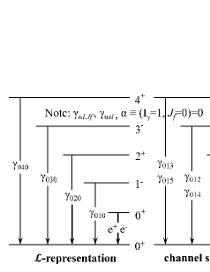
Figure 1: The electric multiploes transition processes to ground state (0⁺) described by channel spin scheme and ${\mathcal{L}}$-representation for ¹⁶O system.

For the comparison of two coupling schemes, Fig. 1 displays the all possible transition processes to the ground-state (J^π = $0^{+}$) of ¹⁶O system. The ground-state transition of ${\mathcal{L}}$-representation, set of components has one value for each decay, which is less than the two components in the channel spin scheme of the Fig. 1, and the relevant photon reduced-width amplitude of this processes only exists one parameter in the collision matrix. Only when the channel capture is considered in ${\mathcal{L}}$-representation, this parameter can be split into internal and asymptotic channel contributions Bark91 ; Azum10 . So the channel spin scheme provides more subsets to denote the ground-state transition and cascade transition, which is extremely beneficial to the interpretation of the observed experimental data more reliable.

II.2 Wave function of compound nucleus ¹⁶O

For the ¹²C($\alpha,\gamma$)¹⁶O reaction, the transition of compound nucleus ¹⁶O, initial radioactive decay to ground state and four bound states are regarded as two body particle reaction channels, denoted by $\gamma$_n+¹⁶O_n (n=0, 1, 2, 3, 4), and the reduced masses of these channels are represented by relativistic energy. It is not necessary to consider how to decay to the ground state finally, so the problem of ‘particles are created or destroyed’ is avoided. The sum of integral cross sections of each reaction channel $\gamma$_n+¹⁶O_n is equal to the cross section of ¹⁶O production.

Owing to the advantage of the channel spin scheme, all the channels of the ¹⁶O system are represented as c = ${\alpha sl}$, where s is the channel spin, l is the relative angular momentum of the interacting particle of entrance or exit channels, and $\alpha$ identifies the interacting particle pair. The primary wave function ${\Psi}$ can be unfolded with different exit channels ${{\mathbf{\psi}}}_{c}$. Furthermore ${{\mathbf{\psi}}}_{c}$ can be expended with level wave functions ${X_{\lambda}}$, which have different total angular momentum, parity ${J}^{\pi}$ and ${E}_{\lambda}$. Finally ${\Psi}$ is expressed with Eq. 2.6 (page 283) in Ref. Lane58 :

$$\Psi=\mathop{\sum}\limits_{c}\left[{\mathop{\sum}\limits_{\lambda}\frac{{{X_{\lambda}}{\gamma_{\lambda c}}}}{{{E_{\lambda}}-E}}}\right]D_{c}^{0}.$$ (8)

So the total wave function for the initial state of ¹⁶O can be expanded by the complete orthogonal set, the coefficient of the expanded formula represent the probability of different reaction channel of all sorts of resonance energy state. Eq. (8) demonstrates that, if the primary gamma decay $\gamma$_n+¹⁶O_n as the independent two body reaction channel, the set of level wave function ${X_{\lambda}}$, of the theoretical model contains all types of $\gamma$- transition, whether direct decay to the ground state transition or cascade transition. Using the Eq. (8), one can obtain the fundamental R-matrix relation, the collision matrix, the cross sections and so on.

For the channel $\gamma$_n+¹⁶O_n, the electromagnetic interaction is long range, therefore contributions to the collision matrix for radiative capture reactions can come from large distances. Thus, in addition to the internal contribution to the collision matrix, there should also be channel contributions Bark91 . However, for the chief ground state transition, owing to the large binding energy (7.16 MeV) of the ¹⁶O with respect to the $\alpha$+¹²C threshold, its wave function decreases rapidly when the radius is larger than a certain value. So the internal contribution is strongly dominant, and the external part can be neglected. The results in Refs. Bark91 ; Kett82 prove to be reasonable and effective for this approximation, that the external contribution accounts for lower than 3% at 0.3 MeV. For the cascade transitions, a parameter for the final state can be used to characterize the direct capture process of these transitions(see the parameters table). So a global fitting for whole ¹⁶O system can be done using the standard R-matrix formulae of Ref. Lane58 with a suitable channel radius.

II.3 Mathematical formalism of RAC code

The practical formulae of our RAC code are introduced from the literatures Chen03 ; Carl08 ; Carl09 . On the R-matrix and the reaction cross sections, the codes are strictly compiled in accordance with the formulae of classic literatures Lane58 , without any approximation.

Explicitly, the R-matrix, which represents all the internal information concerning the structure of the compound system, is defined as

$${\bf{R}}^{J}_{\alpha^{\prime}s^{\prime}l^{\prime},\alpha sl}=\mathop{\sum}\limits_{\lambda\mu}^{N}\gamma_{\alpha^{\prime}s^{\prime}l^{\prime}}^{J}\gamma_{\alpha sl}^{J}{A_{\lambda\mu}}{\delta_{J{J_{0}}}},$$ (9)

where $\gamma_{\alpha^{\prime}s^{\prime}l^{\prime}}^{J}$ and $\gamma_{\alpha sl}^{J}$ are the reduced-width amplitude of entrance and exit channel, respectively. The matrix ${{\mathbf{A}}}_{{\mathbf{\lambda}}{\mathbf{\mu}}}$ is defined by its inverse

$${\left[{{A^{-1}}}\right]_{\lambda\mu}}=\left({E_{\lambda}-E}\right){\delta_{\lambda\mu}}-{\Delta}_{\lambda\mu}-\frac{i{\Gamma}_{\lambda\mu}}{2},$$ (10)

where $E_{\lambda}$ is the position of resonance level, ${\Delta}_{\lambda\mu}$ is the energy shift, ${\Gamma}_{\lambda\mu}$ is the total reduced channel width, which can represent the contribution of all un-considered channels, such as the ¹²C($\alpha,\alpha_{2}$)¹²C in our fit. The additional quantity appearing in Eqs. (10) is

$${{\Delta}_{\lambda\mu}}=-\mathop{\sum}\limits_{\alpha sl}^{N}\left({{{S}_{\lambda\mu}}-{{B}_{\lambda\mu}}}\right)\gamma_{\alpha^{\prime}s^{\prime}l^{\prime}}\gamma_{\alpha sl},$$ (11)

where $S_{\lambda\mu}$ is the shift factor calculated at the channel radius, and $B_{\lambda\mu}$ is the constant boundary parameter.

The literature of of Lane and Thomas (Page 273) Lane58 , gives the correction formula on the level width $\Gamma_{\lambda c}$ and level shift $\Delta_{\lambda c}$:

$${\Gamma_{\lambda c}}=2{P_{c}}\gamma_{\lambda c}^{2}/{d_{c}},$$ (12)

$${\Delta_{\lambda c}}=\frac{{{P_{c}}\left({R_{cc}^{0}{P_{c}}}\right)-S_{c}^{0}\left({1-R_{cc}^{0}S_{c}^{0}}\right)}}{{{d_{c}}}}\gamma_{\lambda c}^{2}.$$ (13)

where

$${d_{c}}={\left({1-R_{cc}^{0}S_{c}^{0}}\right)^{2}}+{\left({R_{cc}^{0}{P_{c}}}\right)^{2}}.$$ (14)

Here, $\lambda$ is the level of c reaction channel, $P_{c}$ is the penetration factor and notation zero is the constant background. These formulae are workable only based upon an approximation of single level. RAC is the multi-channel and multi-level R-matrix formula without constant background. When calculating the width and shift of some levels, the calculated values of R-Matrix with remaining levels are taken as the constant background of the level. The observed width can be related to the physical reduced width amplitudes with a formula as follow:

$${\Gamma}_{\lambda c}^{obs}={\Gamma}_{\lambda c}\left({1+\sum\nolimits_{k}{\gamma_{\lambda k}^{2}}\frac{{d{S_{k}}}}{{dE}}}\right)_{{E_{\lambda}}}^{-1}.$$ (15)

The total width for a state $\lambda$ is then the sum

$$\Gamma_{\lambda}^{obs}=\sum_{c}{\Gamma}_{\lambda c}^{obs}.$$ (16)

With the relation between T-matrix and U-matrix of formula

$${T_{\alpha^{\prime}s^{\prime}l^{\prime},asl}^{J}={e^{2i{\omega_{\alpha l}}}}{\delta_{\alpha^{\prime}s^{\prime}l^{\prime},\alpha sl}}-U_{\alpha^{\prime}s^{\prime}l^{\prime},\alpha sl}^{J}},$$ (17)

for a reaction going through $\alpha\to\alpha^{\prime}$ the angle-integrated cross section is given as,

$${\sigma_{\alpha^{\prime},a}}=\frac{\pi}{{k_{\alpha}^{2}}}\mathop{\sum}\limits_{sl^{\prime}s^{\prime}lJ}\frac{{\left({2J+1}\right)}}{{\left({2{I_{1}}+1}\right)\left({2{I_{2}}+1}\right)}}{\left|{T_{\alpha^{\prime}s^{\prime}l^{\prime},asl}^{J}}\right|^{2}},$$ (18)

and ${I}_{1}$ and ${I}_{2}$ are the projectile and target spins, respectively. It should be noted that the above equation does not hold for charged particle elastic scattering.

For the corresponding differential cross section formula, a more rigorous calculation is involved in Ref. Lane58

$$\frac{d\sigma_{\alpha,\alpha{{}^{\prime}}}}{d\Omega_{\alpha{{}^{\prime}}}}=\frac{1}{(2I_{1}+1)(2I_{2}+1)}\sum_{ss{{}^{\prime}}\nu\nu{{}^{\prime}}}|A_{\alpha{{}^{\prime}}s{{}^{\prime}}\nu{{}^{\prime}},\alpha s\nu}(\Omega_{\alpha{{}^{\prime}}})|^{2},$$ (19)

where $A_{\alpha{{}^{\prime}}s{{}^{\prime}}\nu{{}^{\prime}},\alpha s\nu}$ is the amplitudes of the outgoing waves.

$$A_{\alpha{{}^{\prime}}s{{}^{\prime}}\nu{{}^{\prime}},\alpha s\nu}(\Omega_{\alpha^{{}^{\prime}}})=\frac{\sqrt{\pi}}{k_{\alpha}}[-C_{\alpha{{}^{\prime}}}(\theta_{\alpha{{}^{\prime}}})\delta_{\alpha{{}^{\prime}}s{{}^{\prime}}\nu{{}^{\prime}},\alpha s\nu}+i\sum_{JMll{{}^{\prime}}m{{}^{\prime}}}\sqrt{2l+1}(sl\nu 0|JM)(s{{}^{\prime}}l{{}^{\prime}}\nu{{}^{\prime}}m{{}^{\prime}}|JM)T^{J}_{\alpha{{}^{\prime}}s{{}^{\prime}}l{{}^{\prime}},\alpha sl}Y_{m{{}^{\prime}}}^{(l{{}^{\prime}})}(\Omega_{\alpha{{}^{\prime}}})].$$ (20)

Several new quantities have been introduced in Eq. (20) to define the angular dependence of the cross section. The term $-C_{\alpha{{}^{\prime}}}(\theta_{\alpha{{}^{\prime}}})$ represents the Coulomb amplitudes, while $Y_{m^{\prime}}^{(l^{\prime})}$ is the spheric harmonics function.

The transverse character of electromagnetic wave requires that the projections of intrinsic spins of photon can not be zero. For the transition with $\emph{{J}}_{f}$ = 0, when $\nu{{}^{\prime}}$ = 0, the $\gamma$ spin projection is zero. So when using the Eq. (19) to calculate the angular distribution of $\gamma$ decay, as long as ignoring the loop for $\nu{{}^{\prime}}$ = 0, the calculation will not include the contribution of $\gamma$ spin projection component zero. When this method is adopted, the angle-integrated cross section can be described effectively in our fit, but the corresponding differential cross section is not fitted accurately. So in the actual work, the longitudinal contribution of photon is employed to give a precise description for the all available data.

II.4 Covariance statistic and error propagation law

The uncertainty determination of the extrapolated S factor requires an error propagation of all relevant fit parameters through the fit function taking into account the covariances. The theoretical formula about error propagation Smit91 for our R-matrix model fitting is as following:

$${\mathbf{y}}-{\mathbf{y}}_{0}={\mathbf{D}}({\mathbf{P}}-{\mathbf{P}}_{0}),$$ (21)

$${D}_{ki}=(\partial y_{k}/\partial P_{i})_{0}.$$ (22)

Here ${\mathbf{y}}$ refers to vector of calculated values, ${\mathbf{D}}$ to sensitivity matrix, ${\mathbf{P}}$ to vector of R-matrix parameters. Subscript 0 means optimized original value, k and i stand for fitted data and R-matrix parameter, respectively. The covariance matrix of parameter ${\mathbf{P}}$ is

$${\textbf{V}}_{\textbf{P}}=(\textbf{D}^{+}\textbf{V}^{-1}\textbf{D})^{-1}.$$ (23)

Here V refers to covariance matrix of the data to be fitted, and its inversion matrix can be expressed as following:

$$\mathbf{\textbf{V}^{-1}}=\left(\begin{array}[]{cccc}\textbf{V}^{-1}_{1}&{}\hfil&{}\hfil&{0}\\ {}\hfil&\textbf{V}^{-1}_{2}&{}\hfil&{}\hfil\\ {}\hfil&{}\hfil&\ddots&{}\hfil\\ {0}&{}\hfil&{}\hfil&\textbf{V}^{-1}_{k}\end{array}\right),$$ (24)

where V₁, V₂$\cdots$V_k refer to the covariance matrixes of the sub-set data, which are independent with each other. The covariance matrix of calculated values is

$${\textbf{V}}_{\textbf{y}}=\textbf{D}\textbf{V}_{\textbf{P}}\textbf{D}^{+}.$$ (25)

The sensitivity matrix is quite useful in eliminating redundant fit parameters and in understanding which fit parameters are the most effective on the low-energy extrapolation of the S factor as discussed below.

Formula adopted for optimizing with R-matrix fitting is

$$\chi^{2}=({\mathbf{\eta}}-{\mathbf{y}})^{+}{\mathbf{V}}^{-1}({\mathbf{\eta}}-{\mathbf{y}})\Longrightarrow minimum.$$ (26)

Here ${\mathbf{\eta}}$ refers to the vector of experimental data, ${\mathbf{y}}$ refers to the vector of calculated values. Using covariance statistics and error propagation law, it enables us to get accurate expected values and standard deviation of S factor.

In addition the Peelle Pertinent Puzzle (PPP) was corrected by the method used in Carl09 . RAC was used to produce the accurate (error= 1 %) ⁶Li(n,$\alpha$) and ¹⁰B(n,$\alpha$) cross sections, for International Evaluation of Neutron Cross section Standards Carl08 ; Carl09 . And RAC was comprehensively compared with R-Matrix code EDA and SAMMY of USA Carl08 ; Carl09 , the results were highly identical when the same parameters are used. To verify the performance of the R-matrix code of ¹⁶N $\alpha$ spectrum, we repeated the analysis of Ref. Tang10 using their input data, and the same results were obtained. In a word, it is proved that the code RAC is reliable.

III Evaluation and Fit of experimental data

III.1 The construction of reaction channel

Table 2: The reaction channels in our fit including Q-values, radii, the maximum of the orbital angular momentum, and the data, respectively, in the R-matrix calculation. For the capture reaction, Magnetic L-pole radiation is weaker than the corresponding electric L-pole radiation significantly, so the Magnetic transitions are not considered in our fit.

$Channel$	$Q(MeV)$	$R(fm)$	$\emph{l}_{max}$	$Data$
$\alpha+{}^{12}$C	$0.000$	$6.5$	$6$	$AD,^{16}$N
$\gamma_{0}+{}^{16}$O0	$7.162$	$6.5$	$3$	$AD,S_{g.s.}$
$\gamma_{1}+{}^{16}$O1	$1.113$	$6.5$	$1$	$S_{6.05}$
$\gamma_{2}+{}^{16}$O2	$1.032$	$6.5$	$1$	$S_{6.13}$
$\gamma_{3}+{}^{16}$O3	$0.245$	$6.5$	$1$	$S_{6.92}$
$\gamma_{4}+{}^{16}$O4	$0.045$	$6.5$	$1$	$S_{7.12}$
$\alpha_{1}+{}^{12}$C	$-4.438$	$6.5$	$2$	$AD,\sigma$
$p+{}^{15}$N	$-4.968$	$6.5$	$2$	$AD$

Figure 2: (Color online) Level scheme of the ¹⁶O nucleus Till93 . All states relevant for the analysis are indicated.

The observed position, width or life time of ¹⁶O levels are displayed in Fig. 2 up to the 17.5 MeV energy region from Ref. Till93 . The cascade transition data in Ref. Schu11 and Ref. Mate08 reveal several $\gamma$-ray cascade transitions from the $1^{-}$, $3^{-}$ and $2^{+}$ states at $E_{x}$ = 7.12, 11.49 and 11.51 MeV, respectively, which are considered in our fit. Except the level $J^{\pi}$ = $2^{-}$ ($E_{x}$ = 8.872 MeV), the other 31 levels contain $\alpha$+¹²C reaction channel. Based on the level scheme of the ¹⁶O nucleus, the R-matrix analysis of the ¹⁶O compound nucleus considers one particle entrance channel ¹²C+$\alpha$, eight particle exit channels as shown in the Table 2. The R-matrix calculations were performed for $J^{\pi}$ = $0^{+}$ (four real levels, one background level), $J^{\pi}$ = $1^{-}$ (five real levels, one background level), $J^{\pi}$ = $2^{+}$ and $3^{-}$ (seven real levels, and one background level), $J^{\pi}$ = $4^{+}$ (four real levels, one background level), $J^{\pi}$ = $5^{-}$ (two levels, one background level) and $J^{\pi}$ = $6^{+}$ (two real levels). The available data sets cover the energy from $E_{c.m.}$ = 0.9 MeV to $E_{c.m.}$ = 7.5 MeV in this fit, so the parameters above this region are fixed at values determined from the Ref. Till93 .

III.2 Evaluation of experimental data

The basic principle of the data evaluation is that the database can reflect the information of nuclear structure and nuclear reaction accurately and objectively, no matter which is to use the original data or the appropriate amendment. R-matrix fitting requires the experimental data covering full energy region with complete energy points and continuous values, especially in the resonance peak area with the different types of data. Reliable experimental data subset should satisfy the following requirements: In the resonance peak area, the sum of S factor in different reaction channel should be equal to the total S factor; The peak position of the different types of data should be consistent within the range of error; The principal value of different groups should be consistent within the range of uncertainty; The width data of resonance peaks are matched to the implied width information of the other data; The integral value of the differential data should be equal to the corresponding integral data; The integral data of different groups should span a broad energy range with a number of data points and have a good match with each other.

According to the principle of maximum likelihood, a fit to a dataset with many types and large amount of points needs to meet the approximate statistical distribution, so the revisions of some dataset are reasonable. If one experimental point deviates from the expectations obviously, such as the residual error larger than three times of uncertainty, the error of this point can be enlarged with the Letts’ criteria (3$\sigma$ criteria); In the same type of data, if the difference of principal value is far greater than their uncertainties, the error of corresponding data should be amplified in the fitting; If the principal value in one group data deviates from the expected value wholly, the normalization to this dataset is needed in the fitting; If one high precision dataset is selected as the standard data in the evaluation, then some data with systematical deviation should be normalized to the standard data.

III.3 Iterative fit

The fits to the data of ¹⁶O system are iterated, to achieve internal consistency. A file is a fixed record of the original data, which is to provide the original statistical error for the fit. Another file is a dynamic data file recording the evaluation process, which role is to provide the actually used data in fitting and is updated in the iterative process. In the file the original relative data values are replaced with the new normalized value, and the systematic error values are updated by the standard deviation (STD) of the new calculation. And the statistical errors are renewed with the original one at the beginning, but some of them are corrected according to the Letts’ criteria. The ratio of the corresponding data in there two files is the new scaling factor or normalization coefficient. The scaling factor is adjustable in RAC, which is recorded in the parameter file together with the new R-matrix parameters. Fig. 3 shows the flow chart of R-matrix iterative fit procedure.

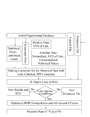
Figure 3: The flow chart for the procedure of iterative fit.

With the continuity of iterative fit, the variation of scaling factor becomes smaller and smaller, and the principal values of relative experimental data are closer to their expectations. Similarly, the R-matrix parameters (RMP), fitted values and their standard deviations become more accurate. At last, all calculated values tend to very slight fluctuations, and the $\chi^{2}$ approaches the minimum.

IV Results and discussion

The following subsections give details of the different reaction channels included in this analysis. Although they are described individually, the fits to the different reaction channel data sets have been performed simultaneously.

IV.1 The reduced $\alpha$-width amplitude for the bound states

At energies of astrophysical interest, direct cross section measurement of capture reaction, such as ¹¹B(p,$\gamma$)¹²C, is very difficult because of the Coulomb barrier, but it can be derived by the proton spectroscopic factor and asymptotic normalization coefficients (ANC) from the transfer reaction ¹²C(¹¹B,¹²C)¹¹B Li14 based on distorted wave Born approximation (DWBA) analysis Du15 ; Canb15 ; Wu14 . The S factor of ¹²C($\alpha$, $\gamma$)¹⁶O at astrophysical energies arises largely from the high-energy tails of subthreshold states $2^{+}_{1}$(Ex = 6.92 MeV) and $1^{-}_{1}$(Ex = 7.12 MeV) of ¹⁶O, but the properties of these states are only weakly constrained by cross-section measurements at higher energies. The cross section of transfer reactions $({}^{6}Li,d)$ and $({}^{7}Li,t)$ provides an alternative way for extracting the reduced $\alpha$-widths for these states of ¹⁶O. In this fit, the $\gamma_{\alpha}$ of $1^{-}_{1}$ and $2^{+}_{1}$ bound states are fixed to the weighted average of two new measurements Belh07 ; Oule12 , and the other subthreshold states, the $\gamma_{\alpha}$ of $0^{+}_{1}$ and $3^{-}_{1}$ are adopted by the literature value of Ref. Oule12 . While the $\gamma_{\gamma}$ of the four states could vary within their uncertainties of literature  Till93 .

IV.2 Total S factor

The available total S factor of ¹²C($\alpha$, $\gamma$)¹⁶O have been obtained in four independent experiments  Schu05 ; Schu11 ; Plag12 ; Fuji13 . Fig. 4 illustrates the corresponding fitted values. In general, the fits are perfect where all the energy levels are accurately described. The measurement of Schürmann et al. Schu05 ; Schu11 in inverse kinematics using the recoil mass separator ERNA allowed to collect data with high precision in a wide energy range, which would make a good restriction to the extrapolation of ground transition, cascade transitions and the total S factor. The data of Ref. Schu05 have not given definite numerical value of three narrow peaks 2${}^{+}_{2}$, 4${}^{+}_{1}$ and 0${}^{+}_{2}$, and the author’s personal communication considers that the relative numerical value is difficult to be determined, so the excitation energies and partial widths are fixed by including in the dataset of pseudo cross section points which were assigned by 50% errors around the resonance peaks.

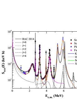
Figure 4: (Color online) Results of the best R-matrix fit for the $S_{tot}$ data from Schürmann 2005: Schu05 , Schürmann 2011: Schu11 , Plag 2012: Plag12 , and Fujita 2013: Fuji13 , together with the decomposition into different energy level contributions. For comparison, the results of Kunz 2002: Kunz02 , Hammer 2005: Hamm05 , Schürmann 2012: Schu12 , and Xu 2013: Xu13 are shown in this figure, respectively.

In the peak region of the 1${}^{-}_{2}$ energy level ($E_{x}$ = 9.58 MeV), the evaluation of data is as follow. We can learn the $S_{tot}$ $\approx$ 97.0 keV b from the measurement of Schürmann et al. Schu05 . The evaluated S${}_{g.s}\approx$ 76.0 is from six groups of S_g.s. Estimating the S_6.05 $\approx$ 1.0 keV b, S_6.92 $\approx$ 7.0 keV b and S_7.12 $\approx$ 20.0 keV b from Ref. Mate06 and Ref. Kunz01 and making assumption for S_6.13 $\approx$ 1.0 keV b. In view of the above, the sum of the partial S factor is 105 keV b , which is 1.08 times of the results $S_{tot}$ = 97 keV b from the measurement of Schürmann et al. Schu05 , that is to say, the experimental value of the total S-factor is significantly less than the sum of the experimental partial S factor. Relevant Ref. Schu05 accounts for that the maximal systemical error is 6.5%, so we choose 1.03 as the normalization coefficient of the data Schu11 in the careful exploration, then the data become S_tot = 100 keV b, which is lower than the sum of partial S factors. The systematical study shows that the S_6.92 of Ref. Kunz01 has an increasing trend, and the S_7.12 of this paper has a decreasing trend. When taking the normalization coefficient of S_6.92 and S_7.12 as 1.00 and 0.95, respectively, then the sum of partial S-factor is approximately equal to 100 keV b. Theresore we can get a satisfied dataset which has complete types and numerical self-consistency for the main resonance peak 1${}^{-}_{2}$. These constitute the skeleton of the whole database for the fits.

Another skeleton of the dataset is the data on the peak region of 2${}^{-}_{3}$ at $E_{c.m.}$ = 4.358 MeV (See Fig. 4). The data of Schürmann et al. Schu11 is obtained by the adding of their components S_g.s, S_6.05, S_6.13, S_6.92 and S_7.12, and it is consistent with the total S factor of Schürmann et al. Schu05 very well. All kinds of the data of Ref. Schu11 are used as the standard data, and the normalization coefficient is 1.03.

Recently, the ¹²C($\alpha$, $\gamma$)¹⁶O cross sections of Plag et al. Plag12 have been measured at four energy points, $E_{c.m.}$ between 1.00 and 1.51 MeV, and the $E10$ and $E20$ components were derived with an accuracy comparable to the previous best data obtained with HPGe detectors. This data are first employed in the $S_{tot}$ fit, which have great influences on the $S_{tot}$(0.3 MeV). In Ref. Fuji13 , total cross section measurements for $E_{c.m.}$= 2.4 and 1.5 MeV were performed at KUTL by using a tandem accelerator. And our fit results are relatively close to the principal values.

In current research on S factor of Ref. Kunz02 ; Hamm05 at higher energies, i.e., at $E_{c.m.}$ $>$ 2.8 MeV, resonance parameters taken from Ref. Till93 were used in their R-matrix fit, in which the published data at high energy, such as $\alpha$ capture measurements of Ref. Broc73 were neglected. So the high-energy resonances from $E_{c.m.}$ = 5 MeV to $E_{c.m.}$ = 6 MeV are overestimated apparently (please see the fit of $S_{g.s.}$). In addition, one should note that in the analysis of Ref. Kunz02 ; Hamm05 there is a clear disagreement at energies around $E_{c.m.}$ = 3 and 4 MeV, where the calculation underestimates total cross-section. The latest results of Ref. Schu12 are consistent with the available experimental data, but the high energy data are not analysed in a similar way of the R-matrix fit. In Ref. Xu13 (NACREII) the total and partial S factors are analyzed with the potential model, where the S factor at $2^{+}_{3}$ ($E_{x}$ = 11.52 MeV) is underestimated by the calculation.

IV.3 ${}^{{\mathbf{1}6}}{{\mathbf{N}}}$ $\alpha$ spectrum

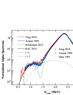
Figure 5: (Color online) Results of the best R-matrix fits (Black line) for the ${}^{{\mathbf{1}6}}{{\mathbf{N}}}$ $\alpha$ spectra from Tang 2010: Tang10 , Azuma 1994: Azum94 , and Zhao 1993: Zhao93 , together with the decomposition into p- (dashed line) and f- wave (dotted line) contributions. For comparison, the best fits of Tang 2010: Tang10 , Azuma 1994: Azum94 , and Schürmann 2012: Schu12 scaled by the corresponding coefficients are shown.

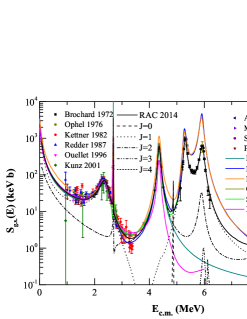
Figure 6: (Color online) Results of the best R-matrix fits for the ground state transitions $S_{g.s.}$ data from Brochard 1972: Broc73 , Ophel 1976: Ophe76 , Kettner 1982: Kett82 , Redder 1987: Redd87 , Ouellet 1996: Ouel96 , Kunz 2001: Kunz01 , Assunção 2006: Assu06 , Makii 2009: Maki09 , Schürmann 2011: Schu11 , Plag 2012: Plag12 , together with the decomposition into different energy level contributions. For comparison, the results of Brune 1999: Brun99 , Kunz 2002: Kunz02 , Hammer 2005: Hamm05 , Schürmann 2012: Schu12 , Oulebsir 2012: Oule12 , and Xu 2013: Xu13 are shown.

The shape of the low-energy part of the $\beta$-delayed $\alpha$ spectrum of ¹⁶N is very sensitive to the $\alpha$ + ¹²C reduced width of the $1^{-}_{1}$ subthreshold state and $1^{-}_{2}$ state of ¹⁶O, in turn, which dominates the low-energy p-wave capture $S_{E10}$(0.3MeV) of ¹²C($\alpha,\gamma_{0}$)¹⁶O₀. In this energy region the reduced $\alpha$ widths are determined by the $\alpha$ spectra and the angular distributions of ¹²C($\alpha,\alpha$)¹²C, which results in the competition with each other in the fit. As shown in Ref. Buch09 , there exists a limitation by the use of ¹²C($\alpha,\alpha$)¹²C data in Ref. Plag87 for obtaining reliable values of S_E10(0.3 MeV). So the ¹⁶N $\alpha$ spectrum may help to give a better confirmation of the reduced $\alpha$ width amplitude of 1${}^{-}_{1}$ and 1${}^{-}_{2}$. Included in this analysis are the three independent $\alpha$ spectra data of Refs. Tang07 ; Tang10 ; Azum94 ; Zhao93 , and the normalization for probability spectrum is used in the practice to reduce the influence of systematical errors. Fig. 5 shows the fit to the normalized ¹⁶N $\alpha$ spectrum together with the decomposition into p- and f-wave contributions, which suggests a significantly negative interference of the bound ${{\rm 1}}^{-}_{1}$ state with the broad ${{\rm 1}}^{-}_{2}$ state that leads to a second peak at $E_{c.m.}$ = 1.1 MeV and a minimum in the vicinity of 1.4 MeV. The dotted line denotes the contribution of 3^- state, which perfectly compensates this negative interference. The fit concluded that the measurement of Azmua et al Azum94 most likely represents the currently closest approximation to the true $\alpha$ spectrum.

IV.4 ¹²C($\alpha,\gamma_{0}$)¹⁶O₀

For the ground state transitions, the secondary data of E₁₀ and E₂₀ multipoles were used in the previous R-matrix analysis independently (Bark91, ; Schu12, ). In general, these secondary data were obtained from the Legendre polynomials fit (Dyer74, ) (page 510) to the angular distributions of ¹²C($\alpha,\gamma_{0}$)¹⁶O₀ measured at many discrete energies. Two methods of analysis (phase fixed or free) are often applied, however, the derived S factors S_E10 and S_E20 are significantly different for the same $\gamma$ angular distributions, see the Fig.12 of Ref. Assu06 , especially for the S_E20.

In our fit, the S_g.s.=S_E10+S_E20 is used for the ground state transition, which the proportion of S_E10 and S_E20 are determined by the R-matrix fit to the relevant $\gamma$ angular distributions. Fig. 6 shows the fit to ${}^{{\rm 12}}{{\rm C}}\left(\alpha{\rm,}{\gamma}_{0}\right){{}^{{\rm 16}}{{\rm O}}}_{0}$ data of ten independent measurements and the calculations of previous works. It is worth mentioning that after the experiments by Dyer and Barnes Dyer74 , Kettner et al Kett82 , and Redder et al Redd87 , a weighted average value $\sigma$ of 47 $\pm$ 3 nb at resonance peak of ${{\rm 1}}^{-}_{2}$ was used to derive a cross section at low energy, this data plays a vital role for the determination of S_g.s., and can be regarded as a criterion for normalizing the experimental data. Even though the S_g.s. of Kettner et al Kett82 deviates systematically from the other data in this resonant region, it is dispensable since it is the only one that has the data points at above 3.0 MeV. It is noteworthy that if the normalization coefficient is fixed by a factor of 0.87, the data of ${{\rm 1}}^{-}_{2}$ peak region is consistent with the other data, meanwhile the data above 3.0 MeV is well consistent with the S_g.s. of Schürmann et al. Schu11 .

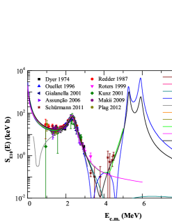
Figure 7: (Color online) The calculation of the $S_{E10}$ with the best R-matrix fit. For comparison, previous fits of Azuma 1994: Azum94 , Ouellet 1996: Ouel96 , Brune 1999: Brun99 , Gialanella 2001: Gial01 , Kunz 2002: Kunz02 , Hammer 2005: Hamm05 , Schürmann 2012: Schu12 , Oulebsir 2012: Oule12 , and Xu 2013: Xu13 are shown in this figure. Data points shown are taken from Dyer 1974: Dyer74 , Redder 1987: Redd87 , Ouellet 1996: Ouel96 , Roters 1999: Rote99 , Kunz 2001: Kunz01 , Gialanella 2001: Gial01 , Assunção 2006: Assu06 , Makii 2009: Maki09 , Schürmann 2011: Schu11 , and Plag 2012: Plag12 .

.

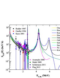
Figure 8: (Color online) The calculation of the $S_{E20}$ with the best R-matrix fit. For comparison, previous fits of Ouellet 1996: Ouel96 , Brune 1999: Brun99 , Kunz 2002: Kunz02 , Hammer 2005: Hamm05 , Dufour 2008: Dufo08 , Oulebsir 2012: Oule12 , Schürmann 2012: Schu12 , Sayre 2012: Sayr12 and Xu 2013: Xu13 are shown in this figure. Data points shown are taken from Redder 1987: Redd87 , Ouellet 1996: Ouel96 , Kunz 2001: Kunz01 , Assunção 2006: Assu06 , Makii 2009: Maki09 , Schürmann 2011: Schu11 , and Plag 2012: Plag12 .

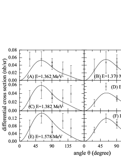
Figure 9: Fits to the ¹²C($\alpha,\gamma_{0}$)¹⁶O₀ angular distributions of Ouellet 1996: Ouel96 at $E_{c.m.}$ = 1.362 (A), 1.370 (B), 1.382 (C), 1.576 (D), 1.578 (E) and 1.580 (F) MeV.

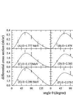
Figure 10: Fits to the ¹²C($\alpha,\gamma_{0}$)¹⁶O₀ angular distributions of Ouellet 1996: Ouel96 at $E_{c.m.}$ = 1.777 (A), 1.979 (B), 2.172 (C), 2.383 (D), 2.390 (E) and 2.570 (F) MeV.

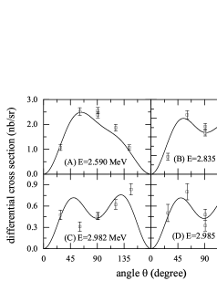
Figure 11: Fits to the ¹²C($\alpha,\gamma_{0}$)¹⁶O₀ angular distributions of Ouellet 1996: Ouel96 at $E_{c.m.}$ = 2.590 (A), 2.835 (B), 2.982 (C) and 2.985 (D) MeV.]

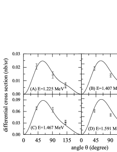
Figure 12: Fits to the ¹²C($\alpha,\gamma_{0}$)¹⁶O₀ angular distributions of Makii 2009: Maki09 at $E_{c.m.}$ = 1.225 (A), 1.470 (B), 1.467 (C), and 1.591 (D) MeV.

In higher energy region, there are five independent experiments Lars64 ; Mitc64 ; Kern71 ; Broc73 ; Ophe76 covering the $1^{-}_{3}$ ($E_{x}$ = 12.44 MeV) and $1^{-}_{4}$ ($E_{x}$ = 13.09 MeV). All the available measurements of the relative ratio of peak cross sections $\sigma$($1^{-}_{3}$) /$\sigma$($1^{-}_{4}$), are tabulated in table 3 of Ref. Ophe76 , in which the largest deviation of Ref. Broc73 data from the other three data, lower about 20%, are evident. So in our fit, the data of Ref. Broc73 near $1^{-}_{4}$ resonance are corrected to the data at the peak of $1^{-}_{3}$ with a factor 0.81. Then the cross sections are found to be in a good agreement with the absolute data from Ref. Ophe76 if normalization corrections (maximum of $\pm$20%) are applied. The remaining data from Ref. Lars64 ; Mitc64 ; Kern71 show good agreement in the shape of the excitation curves, and the normalization factors are given in Table. 3.

The corresponding R-matrix calculation of angular distributions for the reaction ¹²C($\alpha,\gamma_{0}$)¹⁶O₀ are illustrated in Fig. 9- Fig. 22 at representative $\alpha$ energies from $E_{c.m.}$ = 1.002 to $E_{c.m.}$ = 6.075 MeV. The angular distribution measured at the $2^{+}_{2}$ ($E_{x}$ = 9.84 MeV), has the familiar E20 pattern, is symmetric with respect to 90^∘, while the distributions obtained at other energies are asymmetric about 90^∘, clearly indicating the presence of both E10 and E20 amplitudes in the capture mechanism. With the much improved $\gamma$ ray angular distributions in our R-matrix calculation, it can now be possible to derive more accurate values for the cross sections of the E₁₀ and E₂₀ transitions to the ground state of ¹⁶O. Fig. 7 and Fig. 8 show the calculations of the S_E10 and S_E20 together with all the available experimental data. Although the data of S_E10 and S_E20 are not used in the fits, these data lie in two sides of our calculation uniformly, which in turn illustrates the rationality and self-consistency in our R-matrix fit of the angular distributions and S_g.s, ground state transitions.

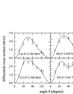
Figure 13: Fits to the ¹²C($\alpha,\gamma_{0}$)¹⁶O₀ angular distributions of Dyer 1974: Dyer74 at $E_{c.m.}$ = 2.180 (A), 2.420 (B), 2.560 (C), and 2.831 (D) MeV.

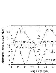
Figure 14: Fits to the ¹²C($\alpha,\gamma_{0}$)¹⁶O₀ angular distributions of Redder 1987: Redd87 at $E_{c.m.}$ = 1.710 (A), 2.360 (B), 2.684 (C), and 2.830 (D) MeV.

In Refs. Ouel96 ; Gial01 the $1^{-}_{1}$ subthreshold state and the $1^{-}_{2}$ resonance may interfere destructively and result in a significantly lower S_E10. However, the constructive solution is strongly favored and the destructive interference pattern has been eliminated in our calculation of angular distribution, resulting in a value of S_E10(0.3 MeV) = 98.0 $\pm$ 7.0 keVb.

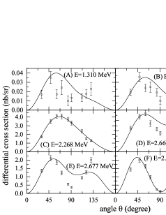
Figure 15: Fits to the ¹²C($\alpha,\gamma_{0}$)¹⁶O₀ angular distributions of Assunção 2006: Assu06 at $E_{c.m.}$ = 1.310 (A), 1.340 (B), 2.268 (C), 2.660 (D), 2.677 (E) and 2.684 (F) MeV.

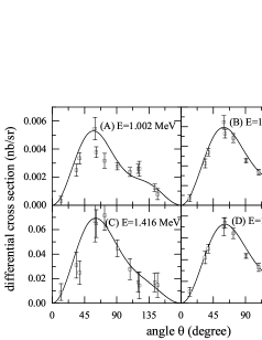
Figure 16: Fits to the ¹²C($\alpha,\gamma_{0}$)¹⁶O₀ angular distributions of Plag 2012: Plag12 at $E_{c.m.}$ = 1.002 (A), 1.308 (B), 1.416 (C) and 1.510 (D) MeV.

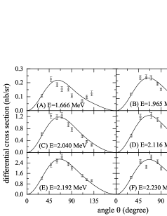
Figure 17: Fits to the ¹²C($\alpha,\gamma_{0}$)¹⁶O₀ angular distributions of Fey 2004: Fey04 at $E_{c.m.}$ = 1.666 (A), 1.965 (B), 2.040 (C), 2.116 (D), 2.192 (E) and 2.230 (F) MeV.

Figure 18: Fits to the ¹²C($\alpha,\gamma_{0}$)¹⁶O₀ angular distributions of Fey 2004: Fey04 at $E_{c.m.}$ = 2.343 (A), 2.455 (B), 2.578 (C), 2.607 (D), 2.652 (E) and 2.682 (F) MeV.

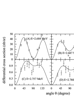
Figure 19: Fits to the ¹²C($\alpha,\gamma_{0}$)¹⁶O₀ angular distributions of Fey 2004: Fey04 at $E_{c.m.}$ = 2.684 (A), 2.687 (B), 2.757 (C) and 2.780 (D) MeV.

Figure 20: Fits to the ¹²C($\alpha,\gamma_{0}$)¹⁶O₀ angular distributions of Kunz 1997: Kunz97 at $E_{c.m.}$ = 2.250 (A), 2.400 (B), 2.480 (C) and 2.684 (D) MeV.

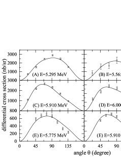
Figure 21: Fits to the ¹²C($\alpha,\gamma_{0}$)¹⁶O₀ angular distributions of Larson 1964: Lars64 and Kernel 1971: Kern71 at $E_{c.m.}$ = 5.295 (A), 5.565 (B), 5.910 (C), 6.000 (D), 5.775 (E) and 5.910 (F) MeV.

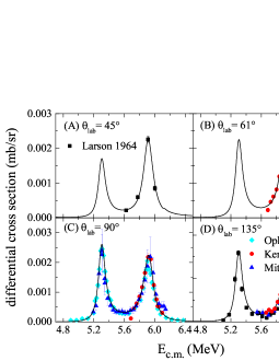
Figure 22: (Color online) Fits to the ¹²C($\alpha,\gamma_{0}$)¹⁶O₀ differential cross-section data at $45^{\circ}$ (A), $61^{\circ}$ (B), $90^{\circ}$ (C), and $135^{\circ}$ (D) from Larson 1964: Lars64 , Kernel 1971: Kern71 , Ophel 1976: Ophe76 and Mitchell 1964: Mitc64 .

The cross section around the $E_{c.m.}$ = 2.5–3.0 MeV region is a rapidly changing function of energy, which strongly depends upon the interference scheme between the resonance $2^{+}_{2}$ and other E₂₀ amplitudes. But the relative E₂₀-E₂₀ interference sign is not well determined by the integral capture data, i.e., the best result of Ref. Schu12 in an interference pattern determined by the high-energy data of Ref. Schu11 is different from most previous analyses Refs. Dufo08 ; Kunz02 . The interference scheme has been commendably constrained by the angular distributions calculation in our R-matrix fitting near this resonance, which are in accordance with the new measurement result of Ref. Sayr12 , and the extrapolation values of S_E20(0.3 MeV) = 56.0 $\pm$ 4.1 keVb in our calculation.

IV.5 ¹²C($\alpha,\gamma_{1}$)¹⁶O₁

Radiative $\alpha$-particle capture into the first excited, J^π = $0^{+}$ state at 6.05 MeV excitation energy have been investigated recently in two independent experiments Schu11 ; Mate06 , however, there exists big differences of S_6.05(0.3 MeV) each other. So it is necessary to give a detailed research and discussion. In the work of C. Matei et.al. Mate06 , S_6.05(0.3 MeV) = $25_{-16}^{+25}$ keV b is obtained by fitting the experimental results therein. It mainly comes from S_E1 and partially from S_E2 and is with large error. In contrast to the analysis of Ref. Mate06 , the extrapolation of Ref. Schu11 suggests a negligible contribution from this amplitude, S_6.05(0.3 MeV) $<$ 1 keV b by analyzing their data, which is mainly contributed by S_E2 while little by S_E1. Ref. Mate06 and Ref. Schu11 use the same experimental method, and both their original data show the $\gamma$ contribution of the first excited state (0${}^{+}_{1}$, 6.05 MeV). But Ref. Schu11 concludes that the S_6.05 is negligible in the energy region less than 3.3 MeV, so it only gives the experimental data above the energy.

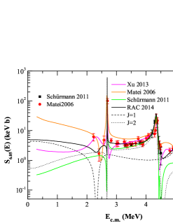
Figure 23: (Color online) Results of best R-matrix fit for the cascade transitions $S_{6.05}$ from Schürmann 2011: Schu11 and Matei 2006: Mate06 , together with the decomposition into different energy level contributions. For comparison, the results of Schürmann 2011: Schu11 , Matei 2006: Mate06 , and Xu 2013: Xu13 are shown in this figure.

In our fit, the data of Ref. Schu11 is regarded as standard data and the normalization coefficient is 1.03. The energy regions of the data in Ref. Mate06 and Ref. Schu11 have overlap around 3.5 MeV. The data of Ref. Mate06 can be normalized by that of Ref. Schu11 , and the normalization factor is 0.88. This forms a dataset of S_6.05 which covers full energy region with complete energy points and continuous values. This transition can therefore be estimated to be S_6.05(0.3MeV) = 4.9 $\pm$ 1.2 keV b, where S_E1 is the most important contribution in S_6.05(0.3 MeV). The S_6.05 obtained by this work is from the systematic analysis of the whole O¹⁶ system. Hence compared with previous analysis, our result is much firmly based on the experiments and is reliable.

IV.6 ¹²C($\alpha,\gamma_{2}$)¹⁶O₂

Very little data exists about the transition into the $E_{x}$ = 6.13 MeV state (J^π = 3^-) except for the 2${}^{+}_{3}$ resonance at $E_{x}$ = 11.60 MeV and 3${}^{-}_{2}$ resonance at $E_{x}$ = 11.52 MeV of Ref. Schu11 . The parameters of these resonance can be sufficient to describe this data and the fit result in S_6.13(0.3 MeV) = 0.2 $\pm$ 0.1 keVb.

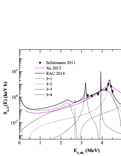
Figure 24: (Color online) Results of the best R-matrix fit for the cascade transitions $S_{6.13}$ from Schürmann 2011: Schu11 together with the decomposition into different energy level contributions. For comparison, the result of Xu 2013: Xu13 is shown in this figure.

IV.7 ¹²C($\alpha,\gamma_{3}$)¹⁶O₃

Four cascade data of S_6.92 Redd87 ; Kett82 ; Kunz01 ; Schu11 cover a range from $E_{c.m.}$ = 1.4 to 5.5 MeV, and the cross section at astrophysical energy is largely governed by the direct capture process, from s-, d- and g-wave captures in Refs. Redd87 ; Kett82 ; Mate08 ; Schu11 . With the reasonable normalization of Refs. Redd87 ; Kett82 , a good fit to these experimental data are achieved from resonance parameters and a direct capture parameter for $J^{\pi}{\rm=}{{\rm 2}}^{{\rm+}}_{1}$ (see parameter table), resulting in S_6.92(0.3 MeV) = 3.0 $\pm$ 0.4 keV b, which is consistent with the result of Ref. Schu12 . Fig. 25 shows the results of S_6.92 as well as its decomposition into different level contributions. Also, the normalization factors are given in Table 3.

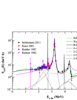
Figure 25: (Color online) Results of the best R-matrix fit for the cascade transitions $S_{6.92}$ from Redder 1987: Redd87 , Kettner 1982: Kett82 , Kunz 2001: Kunz01 , and Schürmann 2011: Schu11 , together with the decomposition into different energy level contributions. For comparison, the results of Schürmann 2012: Schu12 and Xu 2013: Xu13 are shown in this figure.

IV.8 ¹²C($\alpha,\gamma_{4}$)¹⁶O₄

The capture of S_7.12 would be expected to proceed mainly via p- and f-wave direct process and resonance transition at low energies Redd87 ; Schu11 . With resonance parameters and a direct capture parameter for $J^{\pi}{\rm=}{{\rm 1}}^{{\rm-}}_{1}$, a good fit to the experimental data Redd87 ; Kunz01 ; Schu11 is obtained (see parameter table). And the extrapolated S factor for this transition is also small, S_7.12(0.3 MeV) = 0.6 $\pm$ 0.2 keVb. The normalization factors of these applied data are given in Table 3. Fig. 26 shows the results of S_7.12 as well as its decomposition into different level contributions.

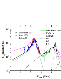
Figure 26: (Color online) Results of the best R-matrix fit for the cascade transitions $S_{7.12}$ from Redder 1987: Redd87 , Kunz 2001: Kunz01 , and Schürmann 2011: Schu11 , together with the decomposition into different energy level contributions. For comparison, the results of Schürmann 2012: Schu12 and Xu 2013: Xu13 are shown in this figure.

IV.9 ¹²C($\alpha,\alpha$)¹²C

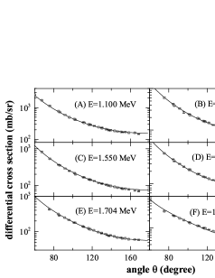
Figure 27: Fits to the ¹²C($\alpha,\alpha$)¹²C angular distributions of Plaga 1987: Plag87 at $E_{c.m.}$ = 1.100 (A), 1.480 (B), 1.550 (C), 1.555 (D), 1.704 (E), and 1.870 (F) MeV.

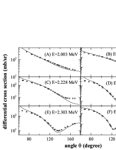
Figure 28: Fits to the ¹²C($\alpha,\alpha$)¹²C angular distributions of Plaga 1987: Plag87 at $E_{c.m.}$ = 2.003 (A), 2.153 (B), 2.228 (C), 2.302 (D), 2.303 (E), and 2.378 (F) MeV.

Figure 29: Fits to the ¹²C($\alpha,\alpha$)¹²C angular distributions of Plaga 1987: Plag87 at $E_{c.m.}$ = 2.452 (A), 2.457 (B), 2.528 (C), 2.588 (D), 2.678 (E), and 2.738 (F) MeV.

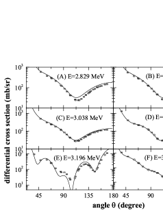
Figure 30: Fits to the ¹²C($\alpha,\alpha$)¹²C angular distributions of Plaga 1987: Plag87 at $E_{c.m.}$ = 2.829 (A), 2.888 (B), 3.038 (C), 3.131 (D), 3.196 (E), and 3.284 (F) MeV.

The most widely used elastic scattering data of $\alpha$-particles on ¹²C contain the $\alpha$ particle information for all relevant states in ¹⁶O, which can be obtained with rather high accuracy. Previous elastic-scattering data have been used to determine the scattering phase shifts for individual angular momenta Refs. Schu12 ; Tang10 and so on. Such a procedure is necessary in cases when the analysis of ¹²C($\alpha$, $\gamma$)¹⁶O is restricted to only one particular angular momentum, but the interference structures in all data, associated with all the resonance states, have been neglected Schu12 ; Buch96 . Taking all angular momenta into account simultaneously, R-matrix fits of four group angular distributions and the associated data Plag87 ; Tisc02 ; Tisc09 ; Morr68 ; Brun75 are presented from $E_{c.m.}$ =1.1 to $E_{c.m.}$ = 5.85 MeV in Fig. 27 to Fig. 38 with the strictly theoretical formulae of Eq. 19. In order to reduce the space of the paper, the figures from $E_{c.m.}$ = 5.85 MeV to $E_{c.m.}$ = 7.5 MeV of Refs. Morr68 ; Brun75 are not shown in this paper.

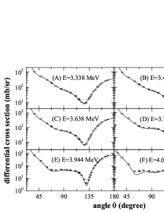
Figure 31: Fits to the ¹²C($\alpha,\alpha$)¹²C angular distributions of Plaga 1987: Plag87 at $E_{c.m.}$ = 3.338 (A), 3.488 (B), 3.638 (C), 3.788 (D), 3.944 (E), and 4.088 (F) MeV.

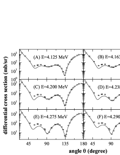
Figure 32: Fits to the ¹²C($\alpha,\alpha$)¹²C angular distributions of Plaga 1987: Plag87 at $E_{c.m.}$ = 4.125 (A), 4.163 (B), 4.200 (C), 4.238 (D), 4.275 (E), and 4.290 (F) MeV.

The scattering data by Plaga et al. Plag87 were obtained in the considerably better energy range in comparing with the other studies. Differential cross-section data for all 35 angles in the range ${\theta}_{lab}$ = 22^∘ to 163^∘ and for 51 energies from $E_{c.m.}$ = 1.0 to 4.9 MeV are included in the fit. Data points in the vicinity of narrow resonances are also contained for this analysis. Level parameters from the fit are in an excellent agreement with those reported in Ref. Till93 . The interference structures in the data, associated with resonance states in the energy range covered by this data, are well reproduced by the R-matrix fits. All the results are shown in Figs.27 to Figs.35.

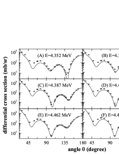
Figure 33: Fits to the ¹²C($\alpha,\alpha$)¹²C angular distributions of Plaga 1987: Plag87 at $E_{c.m.}$ = 4.352 (A), 4.364 (B), 4.387 (C), 4.424 (D), 4.462 (E), and 4.499 (F) MeV.

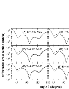
Figure 34: Fits to the ¹²C($\alpha,\alpha$)¹²C angular distributions of Plaga 1987: Plag87 at $E_{c.m.}$ = 4.507 (A), 4.542 (B), 4.582 (C), 4.619 (D), 4.657 (E), and 4.694 (F) MeV.

Recently the angular distributions of ${}^{{\rm 12}}{{\rm C(}\alpha{\rm,}\alpha{\rm)}{}^{{\rm 12}}{{\rm C}}}$ in the $\alpha$-energy range of 2.6–8.2 MeV, at angles from 24^∘ to 166^∘ have been measured at the University of Notre Dame using an array of 32 silicon detectors Tisc02 ; Tisc09 . The relative differential cross-section excitation curves for eight selected detector angles and the four angular distributions for energies near the $E_{c.m.}$ = 2.291 $(1^{-}_{2})$, 3.192 $(4^{+}_{2})$, 3.913 $(2^{+}_{3})$, and 4.902 $(0^{+}_{2})$ MeV resonances are available. To reduce the amount of computations, only the four angular distributions are employed in this fit, which the angular distributions are found to be in a good agreement with those data. Fits are shown in Fig.36.

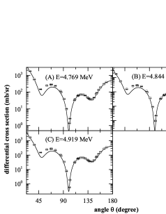
Figure 35: Fits to the ¹²C($\alpha,\alpha$)¹²C angular distributions of Plaga 1987: Plag87 at $E_{c.m.}$ = 4.769 (A), 4.844 (B) and 4.919 (C) MeV.

Figure 36: Fits to the ¹²C($\alpha,\alpha$)¹²C angular distributions of Tischhauser 2009: Tisc09 at $E_{c.m.}$ = 2.291 (A), 3.192 (B), 3.913 (C) and 4.902 (D) MeV.

The best quality $\alpha$-scattering cross-section data above proton separation energies are shown in Fig.37 and Fig.38 of Ref. Morr68 , which have good coherence to experimental data.

Figure 37: Fits to the ¹²C($\alpha,\alpha$)¹²C angular distributions of Morris 1968: Morr68 at $E_{c.m.}$ = 4.950 (A), 5.163 (B), 5.224 (C), 5.243 (D), 5.298 (E) and 5.320 (F) MeV.

Figure 38: Fits to the ¹²C($\alpha,\alpha$)¹²C angular distributions of Morris 1968 Morr68 at $E_{c.m.}$ = 5.375 (A), 5.550 (B), 5.625 (C), 5.775 (D), 5.825 (E) and 5.850 (F) MeV.

IV.10 ¹²C($\alpha,\alpha$₁)¹²C and ¹²C($\alpha,p$)¹⁵N

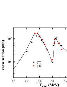
Figure 39: (Color online) Fits to the ¹²C($\alpha,\alpha$₁)¹²C cross section of Mitchell 1965: Mitc65 and deBoer 2012: Debo12a .

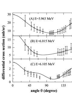
Figure 40: Fits to the ¹²C($\alpha,\alpha$₁)¹²C angular distributions of Mitchell 1965: Mitc65 at $E_{c.m.}$ = 5.963 (A), 6.015 (B) and 6.105 (C) MeV.

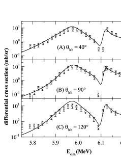
Figure 41: Fits to the ¹²C($\alpha,\alpha$₁)¹²C differential cross section data of Mitchell 1965: Mitc65 .

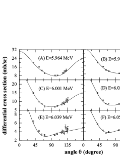
Figure 42: Fits to the ¹²C($\alpha,\alpha$₁)¹²C angular distributions of deBoer 2012: Debo12a at $E_{c.m.}$ = 5.964 (A), 5.984 (B), 6.001 (C), 6.020 (D), 6.039 (E) and 6.059 (F) MeV.

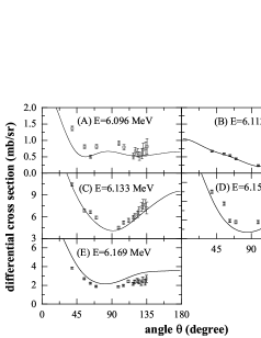
Figure 43: Fits to the ¹²C($\alpha,\alpha$₁)¹²C angular distributions of deBoer 2012: Debo12a at $E_{c.m.}$ = 6.096 MeV (A), 6.113 (B), 6.133 (C), 6.153 (D) and 6.169 (E) MeV.

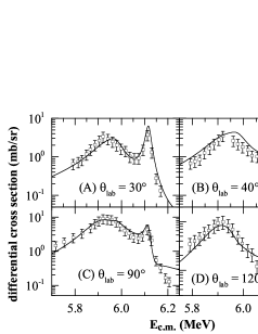
Figure 44: Fits to the ¹²C($\alpha,p$)¹⁵N differential cross section data of Mitchell 1965: Mitc65 .

Good fits of ¹²C($\alpha,{\alpha}_{1}$)¹²C and ¹²C($\alpha,p$)¹⁵N are helpful to reduce the uncertainty produced by the distant levels, and then to improve the fit precision of ¹²C($\alpha,\gamma$)¹⁶O S factor subsequently. Previously, the only available angular distribution data of the ¹²C($\alpha,{\alpha}_{1}$)¹²C reaction has been obtained at incident energies E_c.m. = 5.963, 6.015 and 6.105 MeV in Ref. Mitc65 . And the excitation curves of ¹²C($\alpha,{\alpha}_{1}$)¹²C and ¹²C($\alpha,p$)¹⁵N for four selected detector angles have been measured in the same energy range in the paper. But an absolute scaling was not reported in these measurements. In Ref. Debo12a ; Debo12b , new yield-ratio data for the reactions ¹²C($\alpha,{\alpha}_{1}$)¹²C and ¹²C($\alpha,p$)¹⁵N were performed at the University of Notre Dame in order to provide additional data for a comprehensive R-matrix analysis of compound-nucleus reactions populating ¹⁶O. The data are in the form of yield ratios where the ¹²C($\alpha,{\alpha}_{0}$)¹²C yields measured at an angle ${\theta}_{{\rm lab}}$ = 58.9^∘ are used as the reference data. And the transformational angular distribution data and cross sections are obtained by a private communication with Dr. R. J. deBoer.

The R-matrix fits of ¹²C($\alpha,{\alpha}_{1}$)¹²C angle-integrated cross section are shown by the solid lines in Fig.39, illustrating the consistency level of the simultaneous fit to the data of Ref. Debo12a together with the relative data in Ref. Mitc65 . Fits of the available angular distribution data are shown in Fig.40 to Fig.43, in which the significant contributions originate from states at E${}_{\textrm{x}}$ = 12.95 $(2^{+}_{4})$, 13.13 $(3^{-}_{3})$, and 13.27 $(3^{-}_{4})$ MeV. Fits for the angular distribution data of Ref. Mitc65 for the reaction ¹²C($\alpha,p$)¹⁵N are shown in Fig.44, and the normalization factors are given in Table 3.

Table 3: Scaling factors for datasets which have no reported absolute scale, and the normalization coefficient for the absolute data.

Figure No.	Ref.	Normalization	$\chi^{2}_{C}$	$ndp$	Figure No.	Ref.	Normalization	$\chi^{2}_{C}$	$ndp$
$4$	$[7]$	$1.03\times 10^{+00}$	$1.437$	$91$	$19(B)$	$[17]$	$1.29\times 10^{-08}$	$3.993$	$9$
$4$	$[8]$	$1.03\times 10^{+00}$	$0.959$	$7$	$19(C)$	$[17]$	$1.08\times 10^{-08}$	$1.712$	$9$
$4$	$[10]$	$1.00\times 10^{+00}$	$1.056$	$2$	$19(D)$	$[17]$	$1.25\times 10^{-08}$	$1.060$	$9$
$4$	$[9]$	$1.03\times 10^{+00}$	$4.196$	$4$	$16(A)$	$[9]$	$2.21\times 10^{-10}$	$2.472$	$12$
$5$	$[26]$	$1.00\times 10^{+00}$	$1.406$	$93$	$16(B)$	$[9]$	$3.13\times 10^{-10}$	$2.357$	$12$
$5$	$[27]$	$1.00\times 10^{+00}$	$1.406$	$91$	$16(C)$	$[9]$	$2.20\times 10^{-09}$	$0.384$	$12$
$5$	$[28]$	$1.00\times 10^{+00}$	$1.406$	$75$	$16(D)$	$[9]$	$4.33\times 10^{-10}$	$1.526$	$12$
$27-31$	$[32]$	$1.00\times 10^{+00}$	$1.763$	$823$	Not shown	$[9]$	$1.74\times 10^{-08}$	$3.088$	$12$
$32-35$	$[32]$	$1.00\times 10^{+00}$	$1.185$	$794$	$14(A)$	$[12]$	$7.10\times 10^{-08}$	$2.800$	$6$
$36$	$[34]$	$1.00\times 10^{+00}$	$1.652$	$128$	$14(B)$	$[12]$	$1.50\times 10^{-06}$	$2.806$	$6$
$37,38$	$[35]$	$1.00\times 10^{+00}$	$1.034$	$613$	$14(C)$	$[12]$	$1.18\times 10^{-05}$	$2.145$	$6$
Not shown	$[36]$	$1.00\times 10^{+00}$	$1.060$	$244$	$14(D)$	$[12]$	$3.04\times 10^{-07}$	$1.744$	$6$
$6$	$[12]$	$1.00\times 10^{+00}$	$2.690$	$24$	$21(A)$	$[19]$	$1.93\times 10^{-06}$	$3.672$	$7$
$6$	$[8]$	$1.03\times 10^{+00}$	$2.327$	$7$	$21(B)$	$[19]$	$2.21\times 10^{-06}$	$1.006$	$7$
$6$	$[13]$	$9.70\times 10^{-01}$	$1.753$	$9$	$21(C)$	$[19]$	$1.96\times 10^{-06}$	$2.862$	$7$
$6$	$[16]$	$1.00\times 10^{+00}$	$0.464$	$20$	$21(D)$	$[19]$	$2.12\times 10^{-06}$	$1.536$	$7$
$6$	$[15]$	$1.00\times 10^{+00}$	$0.788$	$20$	$21(E)$	$[21]$	$1.28\times 10^{-06}$	$2.867$	$7$
$6$	$[9]$	$1.03\times 10^{+00}$	$0.784$	$4$	$21(F)$	$[21]$	$1.37\times 10^{-06}$	$2.415$	$7$
$6$	$[18]$	$1.03\times 10^{+00}$	$2.467$	$4$	Not shown	$[21]$	$1.90\times 10^{-06}$	$1.264$	$7$
$6$	$[23]$	$8.70\times 10^{-01}$	$1.196$	$48$	$21(C)$	$[20]$	$1.10\times 10^{+00}$	$2.980$	$40$
$6$	$[67]$	$8.00\times 10^{-01}$	$1.936$	$24$	$22(A)$	$[19]$	$2.02\times 10^{-06}$	$1.261$	$4$
$6$	$[20]$	$1.00\times 10^{+00}$	$0.001$	$1$	$22(D)$	$[19]$	$1.99\times 10^{-06}$	$2.819$	$20$
$9-11$	$[13]$	$9.70\times 10^{-01}$	$1.897$	$96$	$22(B)$	$[21]$	$1.53\times 10^{-06}$	$2.176$	$13$
$12$	$[18]$	$1.03\times 10^{+00}$	$2.346$	$14$	$22(C)$	$[21]$	$1.44\times 10^{-06}$	$1.659$	$13$
$15(A)$	$[16]$	$5.30\times 10^{-10}$	$1.675$	$9$	$22(D)$	$[21]$	$2.12\times 10^{-06}$	$1.267$	$13$
$15(B)$	$[16]$	$4.14\times 10^{-10}$	$1.683$	$9$	$22(C)$	$[22]$	$6.38\times 10^{-05}$	$0.785$	$29$
$15(C)$	$[16]$	$4.68\times 10^{-09}$	$1.089$	$9$	$22(D)$	$[22]$	$1.02\times 10^{-03}$	$1.531$	$14$
$15(D)$	$[16]$	$6.15\times 10^{-09}$	$4.002$	$9$	$23$	$[24]$	$8.00\times 10^{-01}$	$2.276$	$32$
$15(E)$	$[16]$	$5.41\times 10^{-09}$	$4.872$	$9$	$23$	$[8]$	$1.03\times 10^{+00}$	$0.888$	$7$
$15(F)$	$[16]$	$1.31\times 10^{-07}$	$2.576$	$9$	$24$	$[8]$	$1.03\times 10^{+00}$	$1.379$	$7$
$20(A)$	$[14]$	$2.36\times 10^{-06}$	$1.730$	$9$	$25$	$[15]$	$1.00\times 10^{+00}$	$1.076$	$16$
$20(B)$	$[14]$	$2.01\times 10^{-06}$	$1.784$	$9$	$25$	$[12]$	$3.62\times 10^{-01}$	$0.745$	$25$
$20(C)$	$[14]$	$1.48\times 10^{-06}$	$1.328$	$9$	$25$	$[23]$	$3.53\times 10^{-01}$	$2.155$	$21$
$20(D)$	$[14]$	$3.39\times 10^{-06}$	$2.857$	$9$	$25$	$[8]$	$1.03\times 10^{+00}$	$1.268$	$7$
$13(A)$	$[11]$	$9.23\times 10^{-08}$	$1.884$	$10$	$26$	$[15]$	$1.00\times 10^{+00}$	$1.579$	$16$
$13(B)$	$[11]$	$9.16\times 10^{-08}$	$2.213$	$10$	$26$	$[12]$	$4.42\times 10^{-01}$	$2.199$	$25$
$13(C)$	$[11]$	$8.16\times 10^{-08}$	$1.543$	$10$	$26$	$[8]$	$1.03\times 10^{+00}$	$0.492$	$7$
$13(D)$	$[11]$	$6.98\times 10^{-08}$	$1.643$	$10$	$39$	$[37]$	$1.70\times 10^{-02}$	$1.560$	$11$
$17(A)$	$[17]$	$5.08\times 10^{-10}$	$4.156$	$9$	$39$	$[38]$	$1.00\times 10^{+00}$	$0.380$	$11$
$17(B)$	$[17]$	$6.49\times 10^{-10}$	$2.460$	$8$	$40$	$[37]$	$3.66\times 10^{+00}$	$0.037$	$17$
$17(C)$	$[17]$	$2.01\times 10^{-09}$	$2.533$	$9$	$40$	$[37]$	$3.60\times 10^{+00}$	$0.068$	$12$
$17(D)$	$[17]$	$3.42\times 10^{-09}$	$0.942$	$8$	$40$	$[37]$	$1.52\times 10^{-01}$	$0.658$	$16$
$17(E)$	$[17]$	$2.53\times 10^{-09}$	$1.599$	$9$	$41$	$[37]$	$5.54\times 10^{+00}$	$0.829$	$21$
$17(F)$	$[17]$	$3.93\times 10^{-09}$	$1.708$	$9$	$41$	$[37]$	$5.32\times 10^{+00}$	$0.834$	$25$
$18(A)$	$[17]$	$4.67\times 10^{-09}$	$2.490$	$8$	$41$	$[37]$	$5.58\times 10^{-01}$	$1.079$	$21$
$18(B)$	$[17]$	$5.66\times 10^{-09}$	$3.480$	$9$	$42$	$[38]$	$1.00\times 10^{+00}$	$2.078$	$153$
$18(C)$	$[17]$	$1.67\times 10^{-08}$	$1.960$	$9$	$44$	$[37]$	$4.20\times 10^{+00}$	$0.804$	$21$
$18(D)$	$[17]$	$3.83\times 10^{-09}$	$2.645$	$9$	$44$	$[37]$	$2.12\times 10^{+00}$	$0.778$	$20$
$18(E)$	$[17]$	$9.17\times 10^{-09}$	$2.877$	$9$	$44$	$[37]$	$1.48\times 10^{+00}$	$0.877$	$24$
$18(F)$	$[17]$	$1.19\times 10^{-07}$	$1.970$	$9$	$44$	$[37]$	$1.10\times 10^{+00}$	$0.696$	$21$
$19(A)$	$[17]$	$2.53\times 10^{-08}$	$4.693$	$9$

Table 4: Parameters obtained from the R-matrix fits, particle partial widths for the levels, and the radiation widths for the $\gamma$ -ray transitions considered in this work compared with those from literatures.

Res. no.	$E_{x}$(MeV)	$J^{\pi}_{n}$	$E_{\lambda}$(MeV)	$\alpha(I_{1}+I_{2})$	$(s,l)$	$\gamma_{\alpha sl}$(MeV)1/2	$\Gamma$(keV)	Ref. Till93
$01$	$6.049$	$0^{+}_{1}$	$-0.1113$	$\alpha+^{12}$C	$(0,0)$	$-1.37(18)\times 10^{-1}$	$Fixed$	$19.7(55)$
				$\gamma_{0}+^{16}$O0	$(1,1)$	$2.14(41)\times 10^{-5}$	$6.88(50)\times 10^{-12}$	$6.86(50)\times 10^{-12}$
$02$	$12.049$	$0^{+}_{2}$	$4.865$	$\alpha+^{12}$C	$(0,0)$	$4.99(151)\times 10^{-3}$	$1.02(25)\times 10^{0}$	$1.5(5)\times 10^{0}$
				$\gamma_{0}+^{16}$O0	$(1,1)$	$6.25(247)\times 10^{-4}$
$03$	$14.032$	$0^{+}_{3}$	$6.557$	$\alpha+^{12}$C	$(0,0)$	$1.65(5)\times 10^{-1}$	$Fixed$	$\Gamma_{\alpha}/\Gamma_{TOT}=0.9$
$04$	$15.066$	$0^{+}_{4}$	$7.904$	$\alpha+^{12}$C	$(0,0)$	$4.33\times 10^{-1}$	$Fixed$	$\Gamma_{\alpha}/\Gamma_{TOT}=0.35$
				$\alpha_{1}+^{12}$C	$(2,2)$	$5.91\times 10^{-2}$	$Fixed$	$\Gamma_{TOT}=166(30)$
				$p+^{15}$N	$(1,1)$	$-2.85\times 10^{-2}$	$Fixed$
$05$	$BG$	$0^{+}_{5}$	$30.740$	$\alpha+^{12}$C	$(0,0)$	$2.23(9)\times 10^{0}$
				$\gamma_{0}+^{16}$O0	$(1,1)$	$-3.01(20)\times 10^{-4}$
$06$	$7.119$	$1^{-}_{1}$	$-0.4515$	$\alpha+^{12}$C	$(0,1)$	$-8.08\times 10^{-2}$	$Fixed$	$62.0(170)$
				$\gamma_{0}+^{16}$O0	$(1,0)$	$2.20(107)\times 10^{-4}$	$5.7(3)\times 10^{-5}$	$5.5(3)\times 10^{-5}$
				$\gamma_{0}+^{16}$O0	$(1,2)$	$1.61(46)\times 10^{-2}$
				$\gamma_{1}+^{16}$O1	$(1,0)$	$-2.06(898)\times 10^{-6}$	$3.0(1)\times 10^{-10}$	$<3.0\times 10^{-10}$
				$\gamma_{2}+^{16}$O2	$(2,1)$	$-7.32(83)\times 10^{-4}$	$4.5(1)\times 10^{-8}$	$4.6(10)\times 10^{-8}$
				$\gamma_{3}+^{16}$O3	$(1,0)$	$5.54(1300)\times 10^{-6}$	$5.5(2)\times 10^{-10}$	$<1.0\times 10^{-9}$
				$\gamma_{4}+^{16}$O4	$(0,1)$	$-1.00(67)\times 10^{-2}$
$07$	$9.585$	$1^{-}_{2}$	$2.295$	$\alpha+^{12}$C	$(0,1)$	$3.37(3)\times 10^{-1}$	$322(5)$	$420(20)$
				$\gamma_{0}+^{16}$O0	$(1,0)$	$-7.37(25)\times 10^{-5}$	$7.25(23)\times 10^{-6}$	$1.56(12)\times 10^{-5}$
				$\gamma_{0}+^{16}$O0	$(1,2)$	$-2.99(9)\times 10^{-3}$
				$\gamma_{1}+^{16}$O1	$(1,0)$	$-1.39(15)\times 10^{-4}$
				$\gamma_{3}+^{16}$O3	$(1,0)$	$-6.46(45)\times 10^{-5}$	$5.8(8)\times 10^{-7}$	$1.4(14)\times 10^{-6}$
				$\gamma_{4}+^{16}$O4	$(0,1)$	$1.36(68)\times 10^{-3}$	$1.5(15)\times 10^{-6}$	$7.8(16)\times 10^{-6}$
$08$	$12.442$	$1^{-}_{3}$	$5.289$	$\alpha+^{12}$C	$(0,1)$	$1.13(2)\times 10^{-1}$	$162(7)$	$102(4)$
				$\gamma_{0}+^{16}$O0	$(1,0)$	$-8.15(137)\times 10^{-4}$	$2.3(3)\times 10^{-3}$	$1.2(2)\times 10^{-2}$
				$\gamma_{0}+^{16}$O0	$(1,2)$	$-2.73(13)\times 10^{-2}$
				$\gamma_{1}+^{16}$O1	$(1,0)$	$-5.25(59)\times 10^{-4}$	$1.2(3)\times 10^{-4}$	$1.2(6)\times 10^{-4}$
				$\gamma_{2}+^{16}$O2	$(2,1)$	$1.39(51)\times 10^{-3}$	$3.4(25)\times 10^{-5}$	$7.0(30)\times 10^{-5}$
				$\gamma_{4}+^{16}$O4	$(0,1)$	$2.89(55)\times 10^{-3}$	$9.0(34)\times 10^{-5}$	$1.3(5)\times 10^{-4}$
				$\alpha_{1}+^{12}$C	$(2,1)$	$1.12(4)\times 10^{-1}$	$2.9(2)\times 10^{-2}$	$2.5\times 10^{-2}$
				$p+^{15}$N	$(1,0)$	$1.16(10)\times 10^{-1}$	$1.8(3)\times 10^{-1}$	$9.0(1)\times 10^{-1}$
$09$	$13.088$	$1^{-}_{4}$	$5.859$	$\alpha+^{12}$C	$(0,1)$	$-4.71(49)\times 10^{-2}$	$27(4)$	$45(18)$
				$\gamma_{0}+^{16}$O0	$(1,0)$	$-3.56(52)\times 10^{-3}$	$1.20(4)\times 10^{-2}$	$3.2(5)\times 10^{-2}$
				$\gamma_{0}+^{16}$O0	$(1,2)$	$-2.42(14)\times 10^{-2}$
				$\gamma_{1}+^{16}$O1	$(1,0)$	$-7.77(118)\times 10^{-4}$	$2.7(8)\times 10^{-4}$	$2.4(5)\times 10^{-4}$
				$\gamma_{2}+^{16}$O2	$(2,1)$	$-3.54(86)\times 10^{-3}$	$2.8(13)\times 10^{-4}$	$4.0(20)\times 10^{-4}$
				$\gamma_{4}+^{16}$O4	$(0,1)$	$-9.53(136)\times 10^{-3}$	$1.3(4)\times 10^{-3}$	$1.35(40)\times 10^{-3}$
				$\alpha_{1}+^{12}$C	$(2,1)$	$8.30(52)\times 10^{-2}$	$8.5(9)\times 10^{-1}$	$1.0\times 10^{0}$
				$p+^{15}$N	$(1,0)$	$2.35(13)\times 10^{-1}$	$3.4(4)\times 10^{1}$	$1.1(2)\times 10^{2}$
$10$	$17.510$	$1^{-}_{5}$	$9.710$	$\alpha+^{12}$C	$(0,1)$	$-8.99(387)\times 10^{-2}$	$Fixed$	$29(9)$
$11$	$BG$	$1^{-}_{6}$	$11.434$	$\alpha+^{12}$C	$(0,1)$	$1.23(1)\times 10^{-2}$
				$\gamma_{0}+^{16}$O0	$(1,0)$	$-5.75(65)\times 10^{-4}$
				$\gamma_{0}+^{16}$O0	$(1,2)$	$7.40(237)\times 10^{-3}$
				$\gamma_{1}+^{16}$O1	$(1,0)$	$-9.71(133)\times 10^{-4}$
				$p+^{15}$N	$(1,0)$	$-8.95(290)\times 10^{-2}$
$12$	$6.917$	$2^{+}_{1}$	$-0.2449$	$\alpha+^{12}$C	$(0,2)$	$1.68\times 10^{-1}$	$Fixed$	$26.7(103)$
				$\gamma_{0}+^{16}$O0	$(1,1)$	$1.99(8)\times 10^{-3}$	$9.9(3)\times 10^{-5}$	$9.7(3)\times 10^{-5}$
				$\gamma_{0}+^{16}$O0	$(1,3)$	$2.81(37)\times 10^{-1}$
				$\gamma_{1}+^{16}$O1	$(1,1)$	$-6.75(5)\times 10^{-4}$	$2.7(3)\times 10^{-8}$	$2.7(3)\times 10^{-8}$
				$\gamma_{2}+^{16}$O2	$(2,0)$	$1.30(29)\times 10^{-5}$	$9.0(30)\times 10^{-9}$	$9.0\times 10^{-9}$
				$\gamma_{3}+^{16}$O3	$(1,1)$	$1.96(23)\times 10^{-2}$

Table 5: Parameters obtained from the R-matrix fits, particle partial widths for the levels, and the radiation widths for the $\gamma$-ray transitions considered in this work compared with those from literatures.

Res. no.	$E_{x}$(MeV)	$J^{\pi}_{n}$	$E_{\lambda}$(MeV)	$\alpha(I_{1}+I_{2})$	$(s,l)$	$\gamma_{\alpha sl}$(MeV)1/2	$\Gamma$(keV)	Ref. Till93
$13$	$9.844$	$2^{+}_{2}$	$2.684$	$\alpha+^{12}$C	$(0,2)$	$1.34(2)\times 10^{-2}$	$0.71(19)$	$0.625(100)$
				$\gamma_{0}+^{16}$O0	$(1,1)$	$-1.62(3)\times 10^{-4}$	$2.0(1)\times 10^{-6}$	$5.7(6)\times 10^{-6}$
				$\gamma_{0}+^{16}$O0	$(1,3)$	$-1.03(3)\times 10^{-2}$
				$\gamma_{1}+^{16}$O1	$(1,1)$	$-3.27(43)\times 10^{-4}$	$4.4(12)\times 10^{-7}$	$1.9(4)\times 10^{-6}$
				$\gamma_{3}+^{16}$O3	$(1,1)$	$-1.03(9)\times 10^{-3}$	$2.1(4)\times 10^{-6}$	$2.2(4)\times 10^{-6}$
$14$	$11.520$	$2^{+}_{3}$	$4.314$	$\alpha+^{12}$C	$(0,2)$	$6.86(3)\times 10^{-2}$	$74(1)$	$71(5)$
				$\gamma_{0}+^{16}$O0	$(1,1)$	$1.77(17)\times 10^{-3}$	$6.8(2)\times 10^{-4}$	$6.1(2)\times 10^{-4}$
				$\gamma_{0}+^{16}$O0	$(1,3)$	$-2.02(15)\times 10^{-2}$
				$\gamma_{1}+^{16}$O1	$(1,1)$	$1.64(13)\times 10^{-3}$	$3.1(5)\times 10^{-5}$	$3.0(5)\times 10^{-5}$
				$\gamma_{2}+^{16}$O2	$(2,0)$	$2.46(16)\times 10^{-4}$	$2.2(3)\times 10^{-5}$	$2.0\times 10^{-5}$
				$\gamma_{3}+^{16}$O3	$(1,1)$	$-1.66(14)\times 10^{-3}$	$2.0(3)\times 10^{-5}$	$2.9(7)\times 10^{-5}$
				$\gamma_{4}+^{16}$O4	$(2,0)$	$-1.90(32)\times 10^{-4}$	$1.1(4)\times 10^{-5}$	$<5.0\times 10^{-6}$
$15$	$13.020$	$2^{+}_{4}$	$5.833$	$\alpha+^{12}$C	$(0,2)$	$8.15(20)\times 10^{-2}$	$112(5)$	$150(10)$
				$\gamma_{0}+^{16}$O0	$(1,1)$	$-8.51(66)\times 10^{-4}$	$2.2(2)\times 10^{-4}$	$7.0(20)\times 10^{-4}$
				$\gamma_{0}+^{16}$O0	$(1,3)$	$-7.54(74)\times 10^{-2}$
				$\alpha_{1}+^{12}$C	$(2,0)$	$-4.04(37)\times 10^{-2}$	$4.1(8)\times 10^{-1}$	$5.0(20)\times 10^{-1}$
				$p+^{15}$N	$(1,1)$	$-8.23(45)\times 10^{-2}$	$1.6(2)\times 10^{0}$	$1.5(2)\times 10^{0}$
$16$	$15.90$	$2^{+}_{5}$	$8.300$	$\alpha+^{12}$C	$(0,2)$	$2.22(9)\times 10^{-1}$	$Fixed$	$\Gamma_{TOT}=600$
				$\gamma_{0}+^{16}$O0	$(1,1)$	$-1.34(8)\times 10^{-3}$	$Fixed$	$\Gamma_{\alpha}\Gamma_{\gamma}/\Gamma_{TOT}=0.4eV$
$17$	$16.443$	$2^{+}_{6}$	$9.281$	$\alpha+^{12}$C	$(0,2)$	$-3.37(26)\times 10^{-2}$	$Fixed$	$\Gamma_{\alpha}/\Gamma_{TOT}=0.28$
				$\gamma_{0}+^{16}$O0	$(1,1)$	$1.38(7)\times 10^{-3}$	$Fixed$	$\Gamma_{\alpha}\Gamma_{\gamma}/\Gamma_{TOT}=0.45eV$
				$\alpha_{1}+^{12}$C	$(2,0)$	$-9.50\times 10^{-3}$	$Fixed$	$\Gamma_{TOT}=22(3)$
				$p+^{15}$N	$(1,1)$	$8.75\times 10^{-3}$	$Fixed$
$18$	$17.129$	$2^{+}_{7}$	$9.967$	$\alpha+^{12}$C	$(0,2)$	$-7.68\times 10^{-2}$	$Fixed$	$\Gamma_{\alpha}/\Gamma_{TOT}=0.37$
				$\alpha_{1}+^{12}$C	$(2,0)$	$6.62\times 10^{-3}$	$Fixed$	$\Gamma_{TOT}=107(14)$
				$p+^{15}$N	$(1,1)$	$1.88\times 10^{-2}$	$Fixed$
$19$	$BG$	$2^{+}_{8}$	$22.618$	$\alpha+^{12}$C	$(0,2)$	$2.22(2)\times 10^{0}$
				$\gamma_{0}+^{16}$O0	$(1,1)$	$1.15(14)\times 10^{-3}$
				$\gamma_{0}+^{16}$O0	$(1,3)$	$1.67(48)\times 10^{-1}$
				$\gamma_{1}+^{16}$O1	$(1,1)$	$1.01(12)\times 10^{-2}$
				$\gamma_{3}+^{16}$O3	$(1,1)$	$3.18(21)\times 10^{-3}$
				$\alpha_{1}+^{12}$C	$(2,0)$	$-4.90(42)\times 10^{0}$
				$p+^{15}$N	$(1,1)$	$-1.35(58)\times 10^{0}$
$20$	$6.1299$	$3^{-}_{1}$	$-0.1032$	$\alpha+^{12}$C	$(0,3)$	$-7.39(17)\times 10^{-2}$	$5.44(25)$	$2.35(80)$
				$\gamma_{0}+^{16}$O0	$(1,2)$	$5.83(31)\times 10^{-4}$	$2.47(7)\times 10^{-8}$	$2.60(13)\times 10^{-8}$
$21$	$11.600$	$3^{-}_{2}$	$3.969$	$\alpha+^{12}$C	$(0,3)$	$3.14(2)\times 10^{-1}$	$718(10)$	$800(100)$
				$\gamma_{2}+^{16}$O2	$(2,1)$	$5.38(3930)\times 10^{-5}$	$2.4(346)\times 10^{-8}$	$1.0\times 10^{-5}$
				$\gamma_{3}+^{16}$O3	$(3,0)$	$-1.05(59)\times 10^{-4}$	$2.8(31)\times 10^{-6}$	$1.0\times 10^{-5}$
				$\gamma_{4}+^{16}$O4	$(2,1)$	$6.13(540)\times 10^{-4}$	$1.6(29)\times 10^{-6}$	$2.0\times 10^{-5}$
$22$	$13.129$	$3^{-}_{3}$	$6.082$	$\alpha+^{12}$C	$(0,3)$	$1.02(3)\times 10^{-1}$	$69(5)$	$90(14)$
				$\gamma_{0}+^{16}$O0	$(1,2)$	$-1.63(79)\times 10^{-3}$	$9.1(30)\times 10^{-6}$	$1.0\times 10^{-5}$
				$\gamma_{2}+^{16}$O2	$(2,1)$	$-1.83(30)\times 10^{-2}$	$7.5(25)\times 10^{-3}$	$8.0\times 10^{0}$
				$\alpha_{1}+^{12}$C	$(2,1)$	$-2.88(30)\times 10^{-1}$	$4.26(32)\times 10^{1}$	$2.09(6)\times 10^{1}$
				$p+^{15}$N	$(1,2)$	$-1.12(119)\times 10^{-3}$	$9.8(6)\times 10^{-1}$	$1.0\times 10^{0}$
$23$	$13.259$	$3^{-}_{4}$	$6.063$	$\alpha+^{12}$C	$(0,3)$	$-3.77(21)\times 10^{-2}$	$13(4)$	$9(4)$
				$\gamma_{2}+^{16}$O2	$(2,1)$	$-1.79(15)\times 10^{-2}$	$8.0(13)\times 10^{-3}$	$9.2(15)\times 10^{-3}$
				$\alpha_{1}+^{12}$C	$(2,1)$	$3.44(15)\times 10^{-2}$	$2.96(36)\times 10^{2}$	$8.2(11)\times 10^{0}$
				$p+^{15}$N	$(1,2)$	$4.43(12)\times 10^{-1}$	$1.6(1)\times 10^{1}$	$4.1\times 10^{0}$
$24$	$14.100$	$3^{-}_{5}$	$7.149$	$\alpha+^{12}$C	$(0,3)$	$-5.154\times 10^{-6}$	$Fixed$	$150(75)$
				$\alpha_{1}+^{12}$C	$(2,1)$	$-1.03(63)\times 10^{-2}$	$Fixed$	$\Gamma_{TOT}=750(200)$
$25$	$15.408$	$3^{-}_{6}$	$8.246$	$\alpha+^{12}$C	$(0,3)$	$-2.57\times 10^{-7}$	$Fixed$	$\Gamma_{\alpha}/\Gamma_{TOT}=0.58$
				$\alpha_{1}+^{12}$C	$(2,1)$	$2.24\times 10^{-1}$	$Fixed$	$\Gamma_{TOT}=133(7)$
				$p+^{15}$N	$(1,2)$	$9.83\times 10^{-6}$

Table 6: Parameters obtained from the R-matrix fits, particle partial widths for the levels, and the radiation widths for the $\gamma$ -ray transitions considered in this work compared with those from the literature.

Res. no.	$E_{x}$(MeV)	$J^{\pi}_{n}$	$E_{\lambda}$(MeV)	$\alpha(I_{1}+I_{2})$	$(s,l)$	$\gamma_{\alpha sl}$(MeV)1/2	$\Gamma$(keV)	Ref. Till93
$26$	$15.828$	$3^{-}_{7}$	$8.266$	$\alpha+^{12}$C	$(0,3)$	$-2.24\times 10^{-1}$	$Fixed$	$\Gamma_{\alpha}/\Gamma_{TOT}=0.21$
				$\alpha_{1}+^{12}$C	$(2,1)$	$1.03\times 10^{-2}$	$Fixed$	$\Gamma_{TOT}=703(113)$
$27$	$BG$	$3^{-}_{8}$	$22.618$	$\alpha+^{12}$C	$(0,3)$	$-1.64(1)\times 10^{0}$
				$\gamma_{4}+^{16}$O4	$(2,1)$	$-1.58(63)\times 10^{-2}$
$28$	$10.361$	$4^{+}_{1}$	$3.196$	$\alpha+^{12}$C	$(0,4)$	$2.17(3)\times 10^{-1}$	$28.4(6)$	$26(3)$
				$\gamma_{0}+^{16}$O0	$(1,3)$	$1.15(2650)\times 10^{-4}$	$5.6(20)\times 10^{-11}$	$5.6(20)\times 10^{-11}$
				$\gamma_{2}+^{16}$O2	$(4,0)$	$4.27(47)\times 10^{-5}$	$4.7(10)\times 10^{-7}$	$<1.0\times 10^{-6}$
				$\gamma_{3}+^{16}$O3	$(3,1)$	$-4.25(33)\times 10^{-3}$	$5.2(8)\times 10^{-5}$	$6.2((6)\times 10^{-5}$
$29$	$11.094$	$4^{+}_{2}$	$3.934$	$\alpha+^{12}$C	$(0,4)$	$9.78(108)\times 10^{-3}$	$0.296(32)$	$0.28(5)$
				$\gamma_{2}+^{16}$O2	$(4,0)$	$1.05(19)\times 10^{-4}$	$3.7(1.3)\times 10^{-6}$	$3.1(13)\times 10^{-6}$
				$\gamma_{3}+^{16}$O3	$(3,1)$	$7.04(82)\times 10^{-4}$	$2.7(6)\times 10^{-6}$	$2.5(6)\times 10^{-6}$
$30$	$13.879$	$4^{+}_{3}$	$6.835$	$\alpha+^{12}$C	$(0,4)$	$-5.00(56)\times 10^{-2}$	$50.3(49)$	$\Gamma_{\alpha}/\Gamma_{TOT}=0.65(5)$
				$\alpha_{1}+^{12}$C	$(2,1)$	$-2.01(14)\times 10^{-1}$	$\Gamma_{TOT}=74(7)$	$\Gamma_{TOT}=77(7)$
$31$	$16.844$	$4^{+}_{4}$	$9.682$	$\alpha+^{12}$C	$(0,4)$	$1.06(21)\times 10^{-1}$	$Fixed$	$\Gamma_{TOT}=567(60),\Gamma_{\alpha}/\Gamma_{TOT}=0.28$
$32$	$BG$	$4^{+}_{5}$	$30.230$	$\alpha+^{12}$C	$(0,4)$	$2.10(3)\times 10^{0}$
				$\gamma_{3}+^{16}$O3	$(3,1)$	$-3.44(30)\times 10^{-2}$
				$\alpha_{1}+^{12}$C	$(2,2)$	$-8.50(118)\times 10^{-1}$
$33$	$14.660$	$5^{-}_{1}$	$7.498$	$\alpha+^{12}$C	$(0,5)$	$3.47\times 10^{-1}$	$Fixed$	$\Gamma_{TOT}=672(11),\Gamma_{\alpha}/\Gamma_{TOT}=0.94$
$34$	$16.900$	$5^{-}_{2}$	$9.748$	$\alpha+^{12}$C	$(0,5)$	$2.9\times 10^{-1}$	$Fixed$	$\Gamma_{\alpha}=700$
$35$	$BG$	$5^{-}_{3}$	$23.514$	$\alpha+^{12}$C	$(0,5)$	$1.21\times 10^{0}$
$36$	$14.805$	$6^{+}_{1}$	$7.657$	$\alpha+^{12}$C	$(0,6)$	$-2.25\times 10^{-1}$	$Fixed$	$\Gamma_{TOT}=70(8),\Gamma_{\alpha}/\Gamma_{TOT}=0.28$
$37$	$16.275$	$6^{+}_{2}$	$9.133$	$\alpha+^{12}$C	$(0,6)$	$2.83\times 10^{-1}$	$Fixed$	$\Gamma_{TOT}=422(14)$

V Summary

This study presents a new R-matrix theory for the ¹²C($\alpha,\gamma$)¹⁶O S factor at helium burning temperature, and a number of applications to demonstrate the applicability and versatility of this theory. The final result of S(0.3 MeV) = 162.7 $\pm$ 7.3 represents the most precise extrapolation of the ¹²C($\alpha,\gamma$)¹⁶O S factor at helium burning temperature based on a set of complementary data including all available information of ¹⁶O system so far. This is to our knowledge the first published analysis meeting the precision requirements on ¹²C($\alpha,\gamma$)¹⁶O. The whole S factor from 0.3 MeV to 10 MeV provides astrophysical reaction rate of ¹²C($\alpha,\gamma$)¹⁶O with a sound basis for researches of nucleosynthesis and evolution of stars.

- (1) C. E. Rolfs and W. S. Rodney, Cauldrons in the Cosmos (The Univ. of Chicago Press, 1988), pp. xi-xii.
- (2) H. O. U. Fynbo et al., Nature 433, 136 (2005).
- (3) W. S. E. Woosley and A. Heger, Phys. Rep. 442, 269 (2007).
- (4) S. M. Austin, A. Heger, and C. Tur, Phys. Rev. Lett. 106, 152501 (2011).
- (5) S. M. Austin, C. West and A. Heger, Phys. Rev. Lett. 112, 111101 (2014).
- (6) C. Tur, A. Heger and S. M. Austin, Astrophys. J. 718, 357 (2010).
- (7) D. Schürmann et al., Eur. Phys. J. A 26, 301 (2005)
- (8) D. Schürmann et al., Phys. Lett. B 703, 557 (2011).
- (9) R. Plag et al., Phys. Rev. C 86, 015805 (2012).
- (10) K. Fujita et al., Few-Body Syst 54, 1603 (2013).
- (11) P. Dyer and C.A. Barnes, Nucl. Phys. A 233, 495 (1974).
- (12) A. Redder, H.W. Becker, C. Rolfs, H.-P. Trautvetter, T.R. Donoghue, T.C. Rinckel, J.W. Hammer, and K. Langanke, Nucl. Phys. A 462, 385 (1987).
- (13) J.M.L. Ouellet, M.N. Butler, H.C. Evans, H.W. Lee, J.R. Leslie, J.D. MacArthur, W. McLatchie, H.-B. Mak, P. Skensved, J.L. Whitton, X. Zhao, and T.K. Alexander, Phys. Rev. C 54, 1982 (1996).
- (14) R. Kunz et al., Nucl. Phys. A 621, 149 (1997).
- (15) R. Kunz, M. Jaeger, A. Mayer, J.W. Hammer, G. Staudt, S. Harissopulos, and T. Paradellis, Phys. Rev. Lett. 86, 3244 (2001).
- (16) M. Assunção et al., Phys. Rev. C 73, 055801 (2006).
- (17) M. Fey, PhD thesis, Stuttgart, Germany 2004, URL: http://elib.uni-stuttgart.de/opus/volltexte/2004/1683.
- (18) H. Makii et al., Phys. Rev. C 80, 065802 (2009).
- (19) J. D. Larson and R. H. Spear, Nucl. Phys. 56, 497 (1964).
- (20) T.R. Ophel, A.D. Frawley, P.B. Treacy, and K.H. Bray, Nucl. Phys. A 273, 397 (1976).
- (21) W. M. G. Kernel and U. von Wimmersperg, Nucl. Phys. A 167, 352 (1971).
- (22) I. V. Mitchell and T. R. Ophel, Nucl. Phys. A 58, 529 (1964).
- (23) K.U. Kettner, H.W. Becker, L. Buchmann, J. Görres, H. Kräwinkel, C. Rolfs, P. Schmalbrock, H.P. Trautvetter and A. Vlieks, Z. Phys. A 308, 73 (1982)
- (24) C. Matei et al., Phys. Rev. Lett. 97, 242503 (2006).
- (25) X. D. Tang et al., Phys. Rev. Lett. 99, 052502 (2007).
- (26) X. D. Tang et al., Phys. Rev. C 81, 045809 (2010).
- (27) R.E. Azuma, L. Buchmann, F.C. Barkeret et al., Phys. Rev. C 50, 1194 (1994), and Phys. Rev. C 56, 1655 (1997).
- (28) Z. Zhao et al., Phys. Rev. Lett. 70, 2066 (1993).
- (29) C.R. Brune, W.H. Geist, R.W. Kavanagh and K.D. Veal, Phys. Rev. Lett. 83, 4025 (1999)
- (30) A. Belhout et al., Nucl. Phys. A ,793, 178 (2007).
- (31) N. Oulebsir et al., Phys. Rev. C 85, 035804 (2012).
- (32) R. Plaga, H.W. Becker, A. Redder, C. Rolfs, H.-P. Trautvetter, and K. Langanke, Nucl. Phys. A 465, 291 (1987).
- (33) P. Tischhauser, R. E. Azuma, L. Buchmann, R. Detwiler, U. Giesen, J. Görres, M. Heil, J. Hinnefeld, F. Käppeler, J. J. Kolata, H. Schatz, A. Shotter, E. Stech, S. Vouzoukas, and M. Wiescher, Phys. Rev. Lett. 88, 072501 (2002).
- (34) P. Tischhauser et al., Phys. Rev. C 79, 055803 (2009).
- (35) J. M. Morris, G. W. Kerr, and T. R. Ophel, Nucl. Phys. A 112, 97 (1968).
- (36) M. Bruno, I. Massa, A. Uguzzoni, G. Vannini, E. Verondini, and A. Vitale, Nuovo Cim., 27, 1 (1975).
- (37) I. V. Mitchell and T. R. Ophel, Nucl. Phys. A 66, 553 (1965).
- (38) R. J. deBoer et al. Phys. Rev. C 85, 045804 (2012).
- (39) R. J. deBoer et al. Phys. Rev. C 85, 038801 (2012).
- (40) D. Schürmann et al., Phys. Lett. B,711, 35 (2012).
- (41) D. B. Sayre, C. R. Brune et al., Phys. Rev. Lett. 109, 142501 (2012).
- (42) C. Matei, C. R. Brune, and T. N. Massey, Phys. Rev. C 78, 065801 (2008).
- (43) J. W. Hammer et al., Nucl. Phys. A ,752, 514c (2005).
- (44) L. Buchmann, R.E. Azuma, C.A. Barnes, J. Humblet, and K. Langanke, Phys. Rev. C 54, 393 (1996).
- (45) UConn-Yale-Duke-Weizmann-PTB-UCL Collaboration, M. Gai et al., J. Phys. Conf. Ser. 337, 012054 (2012).
- (46) K. E. Rehm, J. Phys. Conf. Ser. 337, 012006 (2012).
- (47) Y. Xu et al. Nucl. Instrum. Methods Phys. Res. A 581, 866 (2007).
- (48) A. Lane and R. Thomas, Rev. Mod. Phys. 30, 257 (1958).
- (49) A. Lane, J. Lynn, Nucl. Phys. A 17, 563 (1960).
- (50) F. C. Barker and T. Kajino, Aust. J. Phys. 44, 369 (1991).
- (51) R. J. Holt, H. E. Jackson, R. M. Laszewski, J. E. Monahan, and J. R. Specht, Phys. Rev. C 18, 1962 (1978).
- (52) R. E. Azuma et al., Phys. Rev. C 81, 045805 (2010).
- (53) R. J. deBoer et al., Phys. Rev. C 87, 015802 (2013)
- (54) S. Devons and L. J. B. Goldfarb in Handbuch der Physik, edited by S. Flugge (Springer, Berlin, 1957), Vol. 42, p. 362.
- (55) A. J. Ferguson, Angular Correlation Methods in Gamma- Ray Spectroscopy (North-Holland,Amsterdam1965).
- (56) D. L. Smith, Probability, Statistics, and Data Uncertainties in Nuclear Science and Technology (Amer Nuclear Society, Chicago, 1991).
- (57) Z. P. Chen, R. Zhang et al., Science in China (Series G) 46, 225 (2003).
- (58) A. D. Carlson, S. A. Badikov, Z. P. Chen et al., Nucl. Data Sheets 109, 2834 (2008).
- (59) A. D. Carlson, V.G. Pronyaev, D. L. Smith, N.M. Larson, Z. P. Chen et al., Nucl. Data Sheets 110, 3215 (2009).
- (60) D. R. Tilley, H.R. Weller, and C.M. Cheves, Nucl. Phys. A, 564, 1 (1993).
- (61) E. T. Li, B. Guo, Y. J. Li, Z. H. Li et al., Nuclear Techniques (in Chinese), 37, 100510 (2014).
- (62) X. C. Du, B. Guo, Z. H. Li et al., Sci China-Phys Mech Astron, 58, 062001 (2015).
- (63) B. Canbula et al., Nuclear Science and Techniques, 26, S20504 (2015).
- (64) Z. D. Wu, B. Guo, Z. H. Li et al., Nuclear Techniques (in Chinese), 37, 100512 (2014).
- (65) R. Kunz, M. Fey, M. Jaeger, A. Mayer, J.W. Hammer, G. Staudt, S. Harissopulos, and T. Paradellis, Astrophys. J. 567, 643 (2002).
- (66) Y. Xu et al., Nucl. Phys. A 918, 61 (2013) (NACREII).
- (67) F. Brochard, P. Chevallier, D. Disdier, V. Rauch, and F. Scheibling, J. Phys. France 34, 363 (1973).
- (68) L. Buchmann, G. Ruprecht, and C. Ruiz, Phys. Rev. C 80, 045803 (2009).
- (69) G. Roters, C. Rolfs, F. Strieder, and H. P. Trautvetter, Eur. Phys. J. A 6, 451 (1999).
- (70) L. Gialanella, D. Rogalla, F. Strieder et al., Eur. Phys. J. A 11, 357 (2001)
- (71) M. Dufour and P. Descouvemont, Phys. Rev. C 78, 015808 (2008).