A negative index meta-material for Maxwell’s equations

Abstract

We derive the homogenization limit for time harmonic Maxwell’s equations in a periodic geometry with periodicity length $\eta>0$. The considered meta-material has a singular sub-structure: the permittivity coefficient in the inclusions scales like $\eta^{-2}$ and a part of the substructure (corresponding to wires in the related experiments) occupies only a volume fraction of order $\eta^{2}$; the fact that the wires are connected across the periodicity cells leads to contributions in the effective system. In the limit $\eta\to 0$, we obtain a standard Maxwell system with a frequency dependent effective permeability $\mu^{\mathrm{eff}}(\omega)$ and a frequency independent effective permittivity $\varepsilon^{\mathrm{eff}}$. Our formulas for these coefficients show that both coefficients can have a negative real part, the meta-material can act like a negative index material. The magnetic activity $\mu^{\mathrm{eff}}\neq 1$ is obtained through dielectric resonances as in previous publications. The wires are thin enough to be magnetically invisible, but, due to their connectedness property, they contribute to the effective permittivity. This contribution can be negative due to a negative permittivity in the wires.

Keywords: Maxwell’s equations, negative index material, homogenization

MSC: 78M40, 35B27, 35B34

1 Introduction

Light and other electromagnetic waves exhibit interesting refraction phenomena in meta-materials. While no natural material posesses a negative index, by now, there exists a variety of negative index meta-materials (a meta-material is an assembly of ordinary materials, arranged in small substructures). A smart choice of the microscopic geometry can lead to macroscopic properties of the meta-material that are not shared by any of the ordinary materials that it is made of. Even though no natural negative index material is known, a distribution of metallic or dielectric resonators and metallic wires can act, effectively, as a medium with a negative index. We present here a periodic meta-material (periodicity length $\eta>0$) with singular sub-structures (wires with relative radius of order $\eta$, i.e. with absolute radius of order $\eta^{2}$) which is, on the one hand, close to the experimental set-up, and, on the other hand, accessible to a rigorous mathematical analysis.

From a modelling point of view, the Maxwell system is very simple: We investigate solutions $(E^{\eta},H^{\eta})$ to the time harmonic Maxwell’s equations in three dimensions. The system contains three parameters: the frequency $\omega\in\mathbb{R}$ and two material parameters, the permeability $\mu=\mu(x)$ and the permittivity $\varepsilon=\varepsilon(x)$. Since natural materials have a relative permeability close to one, we assume that the permeability coincides with that of vacuum, $\mu\equiv\mu_{0}>0$. All the complex behavior of the micro-structure is encoded in one single coefficient, the relative permittivity $\varepsilon_{\eta}:\mathbb{R}^{3}\to\mathbb{C}$. Here, we consider periodic coefficients $\varepsilon_{\eta}$ with large values of $|\varepsilon_{\eta}|$ in the inclusions. Using the parameter $\varepsilon_{0}>0$ (permittivity of vacuum), we investigate solutions $(E^{\eta},H^{\eta})$ of

$$\mathrm{curl}\,E^{\eta} =\phantom{-}i\omega\mu_{0}H^{\eta}\,,$$ (1.1)

$$\mathrm{curl}\,H^{\eta} =-i\omega\varepsilon_{\eta}\varepsilon_{0}E^{\eta}\,.$$ (1.2)

Our aim is to analyze the behavior of the solutions $(E^{\eta},H^{\eta})$ in the limit $\eta\to 0$.

The relative permittivity is given by two complex numbers and the geometry of two types of inclusions, $\Sigma_{\eta}\subset\mathbb{R}^{3}$ and $\Gamma_{\eta}\subset\mathbb{R}^{3}$, both periodic with periodicity $\eta$. The set $\Sigma_{\eta}$ consists of bulk inclusions, the number of which is of order $\eta^{-3}$ (one inclusion in each periodicity cell). The set $\Gamma_{\eta}$ represents a system of long and thin wires, each wire has a radius of order $\eta^{2}$ and length of order $1$ (the wire has a macroscopic length and a width that is small compared to the periodicity length). With parameters $\varepsilon_{b},\varepsilon_{w}\in\mathbb{C}$ with $\Im(\varepsilon_{b}),\Im(\varepsilon_{w})>0$ we study the coefficient

$$\varepsilon_{\eta}=\begin{cases}\displaystyle\varepsilon_{b}\eta^{-2}&\text{ in }\Sigma_{\eta}\,,\\[2.84526pt] \displaystyle\varepsilon_{w}\eta^{-2}&\text{ in }\Gamma_{\eta}\,,\\[2.84526pt] 1&\text{ in }\mathbb{R}^{3}\setminus(\Sigma_{\eta}\cup\Gamma_{\eta})\,.\end{cases}$$ (1.3)

Our result is a description of the weak limit $(E,H)$ of a solution sequence $(E^{\eta},H^{\eta})$. We show that an appropriately defined pair $(\hat{E},\hat{H}):=(E,(\hat{\mu})^{-1}H)$ solves a Maxwell system with two effective parameters $\mu^{\mathrm{eff}}(\omega)$ and $\varepsilon^{\mathrm{eff}}$, cp. (1.6)– (1.7). The two effective parameters are given by explicit formulas that involve cell problems for the electric and for the magnetic field. In an appropriate geometry and for an appropriate frequency $\omega$, we find that both coefficients can have a negative real part (simultaneously): The effective permeability $\mu^{\mathrm{eff}}(\omega)$ can become negative due to resonances in the bulk inclusions $\Sigma_{\eta}$. Due to their vanishing volume fraction, the wires do not influence the parameter $\mu^{\mathrm{eff}}(\omega)$. On the other hand, due to their special topology (they form connected objects of macroscopic length), they influence the permittivity $\varepsilon^{\mathrm{eff}}$. If $\varepsilon_{w}$ has a negative real part (which is the case for many metals), then $\varepsilon^{\mathrm{eff}}$ can be negative, see (1.11).

1.1 Literature

Half a century ago, Veselago investigated in the theoretical study [17] materials with negative $\varepsilon$ and negative $\mu$. Since the product $\varepsilon\mu$ is positive, waves can travel in such a medium, but surprising effects such as negative refraction and perfect lensing can be expected. Since no natural materials exhibit a negative $\mu$, the studies of Veselage have not been continued until in about 2000 first ideas were published on how to construct a negative index meta-material, see e.g. [16]. Regarding applications of negative index materials we mention the effect of cloaking by anomalous localized resonance, see e.g. [6] and [14].

A mathematical analysis of meta-materials became possible with the development of the method of homogenization. The homogenization technique was successfully applied in many situations, ranging from porous media to wave equations. Also the homogenization of Maxwell’s equations has been performed. The standard result of a homogenization process is the following: Given periodically oscillating coefficients $a_{\eta}(x)$ and a corresponding solution sequence $u^{\eta}(x)$, every weak limit $u$ of the solution sequence satisfies the original equation with an averaged coefficient $a^{\mathrm{eff}}$. In the context of the Maxwell system, the oscillating coefficients are $a_{\eta}(x)=(\varepsilon_{\eta}(x),\mu_{\eta}(x))$ and the solution is $u^{\eta}=(E^{\eta},H^{\eta})$. In [18], results of this kind are obtained for Maxwell’s equations.

Of particular interest are those homogenization results that lead to a qualitatively different equation for the limit $u$. Examples are the double porosity model in porous media [2] or the dispersive limit equation for waves in heterogeneous media [9, 10]. The problem at hand is similar in that we want to combine positive index materials to obtain an effective negative index material. Typically, such effects are obtained by micro-structures that involve extreme parameter values and/or by micro-structures that contain finer substructures.

In this work, we will actually use both, extreme values and fine substructures, to obtain a surprising new limit formula in the homogenization of Maxwell’s equations. One of the pioneers in the field is Bouchitté who, together with co-authors, initiated the field with the analysis of wire structures [5], [12]. It was shown that extreme coefficient values in the (thin) wires can lead to the effect of a negative $\varepsilon^{\mathrm{eff}}$.

In order to obtain a negative index material, additionally a negative $\mu^{\mathrm{eff}}$ has to be created. Several ideas have been analyzed. Based on the analysis of a model problem, a mathematical result has been obtained in [13]. A truely three-dimensional analysis of a setting that is also close the some of the original designs has been carried out in [7]. In that work, it was shown that the periodic split ring structure can lead to a negative $\mu^{\mathrm{eff}}$. A similar result has been obtained later also for flat rings of arbitrary shape in [15] (while the rings in [7] had to be tori).

While this seems to be the state of the art with regard to metallic inclusions, a simpler approach using dielectric materials has been invented in [4] and later developed in [3]: Dielectric inclusions can lead to resonances (so-called Mie-resonances) which result in an effective magnetic activity. With resonant dielectric inclusions, a negative $\mu^{\mathrm{eff}}$ can be obtained even without subscale variations of the periodic geometry.

With this contribution we close a gap that has been left open by the above mentioned works: The emphasis has always been to create either a negative $\varepsilon^{\mathrm{eff}}$ [5, 12] or a negative $\mu^{\mathrm{eff}}$ [3, 4, 7, 15] — here we present a construction that achieves, simultaneously, a negative $\varepsilon^{\mathrm{eff}}$ and a negative $\mu^{\mathrm{eff}}$ (we always refer to the real part of the coefficient). An important point in our construction is the decoupling: $\varepsilon^{\mathrm{eff}}$ depends only on $\varepsilon_{w}$ and the shape $\Sigma_{Y}$ of the bulk inclusions; given $\Sigma_{Y}$, we can choose $\varepsilon_{w}$ to have $\varepsilon^{\mathrm{eff}}$ negative (independent of the frequency). Tuning the frequency, we can generate a resonance in $\Sigma_{Y}$ which makes $\mu^{\mathrm{eff}}$ negative; this process does not affect $\varepsilon^{\mathrm{eff}}$.

We conclude this section with a comparison of our results to those of [5], where also the effect of thin wires has been analyzed. In [5], the volume fraction $\theta_{\eta}$ of the wires is much smaller than in our study, namely $\theta_{\eta}\sim\exp(-2\eta^{-2})$ (here, it is $\theta_{\eta}\sim\eta^{2}$; we observe that the permittivity is scaled as in our work as $|\varepsilon_{\eta}|\sim\theta_{\eta}^{-1}$). The effective equation in [5] is a Maxwell type system that is coupled to a macroscopic equation for a new variable (denoted by $J$ in [5]). Our result is much simpler in the sense that we obtain a standard Maxwell system in the limit, see (1.6)– (1.7). In this sense, our result is very different to that of [5], despite the similarities in the setting (thin wires with vanishing volume fraction of macroscopic length). In order to understand how such a different outcome is possible, let us mention the following point (somewhat technical, but important): the tiny radii in [5] make it impossible to construct test-functions as in (3.15)–(3.17), hence the macroscopic limit cannot be obtained as in our setting.

1.2 Geometry

The underlying idea of our approach is simple: We use dielectrical bulk-inclusions (given by the subset $\Sigma_{\eta}$) as Mie-resonators, they lead to a negative $\mu^{\mathrm{eff}}$. Additionally, we include thin wires (given by the subset $\Gamma_{\eta}$) that have a negative $\varepsilon$ (which is the case for many metals); the wires lead to a negative $\varepsilon^{\mathrm{eff}}$. Since the wires are thin, their effect decouples from the Mie-resonance.

We emphasize that, defining the two sets $\Sigma_{\eta}$ and $\Gamma_{\eta}$, the Maxwell system is completely described by (1.1)–(1.3). Below, we consider the limit of any bounded solution sequence and do not specify boundary conditions. Our result is therefore applicable to any boundary value problem.

Microscopic geometry.

We construct a periodic meta-material in three space dimensions. We start from the periodicity cube $Y=[0,1)^{3}$; since we will always impose periodicity conditions on the cube $Y$, we may also regard it as the flat torus $\mathbb{T}^{3}$. We now construct two subsets, $\Sigma_{Y},\Gamma_{Y}^{\eta}\subset Y$, compare Figure 1 for an illustration.

Dielectric resonator. The dielectric resonator is given by a subset $\Sigma_{Y}\subset Y$. We assume that $\Sigma_{Y}$ is a simply connected open set that has a Lipschitz boundary and that is compactly contained in $(0,1)^{3}$. We call the set the dielectric resonator since, in order to have resonances in $\Sigma_{Y}$, we must assume that $\varepsilon_{b}$ has a positive real part, cp. (1.10).

Thin wires. The second subset are the (metallic) wires. We assume that three wires $\Gamma_{Y}^{\eta,j}\subset Y$, $j=1,2,3$, are contained in $Y$. We assume that each wire has a radius of order $\eta$ inside $Y$ and that it connects two opposite sides of $\partial Y$ in a periodic fashion. We assume additionally that the wires do not intersect each other or the resonator $\Sigma_{Y}$; this assumption is not satisfied in some of the experimental designs (“fishnet-structure”), but we do not see it as an essential property for our method to work.

In order to make our assumptions precise (and, at the same time, to keep the construction of special test-functions in Section 3 accessible), we restrict ourself to cylindrical wires of relative radius $\alpha>0$: For a point $(y_{1}^{(3)},y_{2}^{(3)})\in(0,1)^{2}$, the wire with index $j=3$ has the central line $\Gamma_{Y}^{3}:=(y_{1}^{(3)},y_{2}^{(3)})\times[0,1)$ and is given by

$$\Gamma_{Y}^{\eta,3}:=B_{\alpha\eta}((y_{1}^{(3)},y_{2}^{(3)}))\times[0,1)\subset Y\,.$$ (1.4)

The wires with indices $1$ and $2$ are constructed accordingly. The union of the three wires is denoted by $\Gamma_{Y}^{\eta}:=\bigcup_{j=1}^{3}\Gamma_{Y}^{\eta,j}$. The construction assures that the relative radius of the wires inside the cube is $\alpha\eta$ such that the wires vanish in the limit $\eta\to 0$. We will see that the wires do not enter the cell problem, but, due to their connectedness across cells, they do affect the macroscopic equations. The real part of the permittivity in the wires has to be negative in order to obtain a negative quantity $\varepsilon^{\mathrm{eff}}$ in (1.11). Since metals can have a negative permittivity, we think of metallic wires.

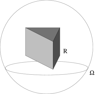
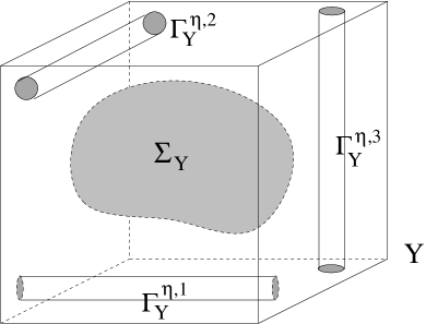
Figure 1: Left: The macroscopic domain $\Omega$ and the scatterer $R\subset\Omega$ (here, $\Omega$ is a ball and $R$ is a prism). Maxwell’s equations are solved on $\Omega$. The equations contain the coefficient $\varepsilon_{\eta}$ which is $1$ in $\Omega\setminus R$ and which has large values and a micro-structure in $R$. Our interest is to describe the solution fields $(E^{\eta},H^{\eta})$ in the limit $\eta\to 0$. Right: The periodicity cell $Y$ with the subsets $\Sigma_{Y}$ (the resonator) and $\Gamma_{Y}^{\eta}$ (the wires). In the two subsets the coefficient $\varepsilon_{\eta}$ has absolute values of order $\eta^{-2}$. The wires have the radius $\alpha\eta$ in the periodicity cell, which means that they have the radius $\alpha\eta^{2}$ in the macroscopic domain. The periodic construction yields connected wires with a length of order $\eta^{0}=1$.

Macroscopic geometry.

We study Maxwell’s equations in an open set $\Omega\subset\mathbb{R}^{3}$. Contained in $\Omega$ is a second domain $R\subset\Omega$ with $\bar{R}\subset\Omega$. The set $R$ consists of the meta-material, on the set $\Omega\setminus R$ we have relative permeability and relative permittivity equal to unity, see Figure 1, left part.

In order to define the microstructure in $R$, we use indices $k\in\mathbb{Z}^{3}$ and shifted small cubes $Y^{\eta}_{k}:=\eta(k+Y)$. We denote by $\mathcal{K}:=\{k\in\mathbb{Z}^{3}|Y^{\eta}_{k}\subset R\}$ the set of indices $k$ such that the small cube $Y^{\eta}_{k}$ is contained in $R$. Here and in the following, in summations or unions over $k$, the index $k$ takes all values in the index set $\mathcal{K}$. The number of relevant indices has the order $|\mathcal{K}|=O(\eta^{-3})$.

Using the local subsets $\Sigma_{Y}$ and $\Gamma^{\eta,j}_{Y}$, we can now define the meta-material by setting

$$\Sigma_{\eta}:=\bigcup_{k\in\mathcal{K}}\eta(k+\Sigma_{Y})\,,\quad\Gamma_{\eta}:=\bigcup_{k\in\mathcal{K}}\bigcup_{j\in\{1,2,3\}}\eta(k+\Gamma^{\eta,j}_{Y})=\bigcup_{k\in\mathcal{K}}\eta(k+\Gamma^{\eta}_{Y})\,.$$ (1.5)

1.3 Main result

With the help of cell-problems, we define two tensors $\varepsilon^{\mathrm{eff}},\mu^{\mathrm{eff}}(\omega)\in\mathbb{C}^{3\times 3}$. The tensor $\varepsilon^{\mathrm{eff}}$ is defined in (1.11) and has two contributions: The matrix $A^{\mathrm{eff}}$ is defined with the standard electrical cell problem, the additive term $\alpha\varepsilon_{w}$ can make the real part of $\varepsilon^{\mathrm{eff}}$ negative. The effective permeability tensor $\mu^{\mathrm{eff}}$ is defined in (2.22) through a coupled cell-problem that appeared already in [3, 7] and was studied there. The formula for $\mu^{\mathrm{eff}}(\omega)$ is a result of the resonance properties of $\Sigma_{Y}$; a negative real part of $\mu^{\mathrm{eff}}(\omega)$ can be expected for frequencies that are close to eigenvalues.

Effective equations.

We derive an effective Maxwell system in $\Omega$:

$$\mathrm{curl}\ \hat{E} =\phantom{-}i\omega\mu_{0}\,\hat{\mu}\hat{H}\,,$$ (1.6)

$$\mathrm{curl}\ \hat{H} =-i\omega\varepsilon_{0}\,\hat{\varepsilon}\hat{E}\,.$$ (1.7)

In this system, the coefficients are $\hat{\mu}(x)=\hat{\varepsilon}(x)=1$ for $x\in\Omega\setminus R$, whereas for $x\in R$

$$\hat{\varepsilon}(x)=\varepsilon^{\mathrm{eff}}\,,\quad\hat{\mu}(x)=\mu^{\mathrm{eff}}(\omega)\,.$$

A consequence of our result is the following: Since outside the scatterer $R\subset\Omega$ the effective coefficients are equal to $1$, the field $(\hat{E},\hat{H})$ coincides there with the weak limit $(E,H)$. In particular, for $x\in\Omega\setminus R$, as $\eta\to 0$, the solutions $(E^{\eta},H^{\eta})$ converge to $(\hat{E},\hat{H})$, solution to the effective system (1.6)–(1.7). Let us now formulate the precise statement in our main theorem.

Theorem 1.1.

Let $(E^{\eta},H^{\eta})$ be a sequence of solutions to (1.1)–(1.2), where the coefficient $\varepsilon_{\eta}$ is given by (1.3) and the geometry of inclusions $\Sigma_{\eta}$ and wires $\Gamma_{\eta}$ is as described above, cf. (1.4) and (1.5). We assume that the solution sequence satisfies the energy-bound

$$\int_{\Omega}|H^{\eta}|^{2}+|\varepsilon_{\eta}|\,|E^{\eta}|^{2}\leq C\,,$$ (1.8)

where $C$ does not depend on $\eta$, and that $(E^{\eta},H^{\eta})$ converges weakly in $L^{2}(\Omega)$ to a limit $(E,H)$. Then the limit $(E,H)$ has the property that the modified fields $\hat{E}:=E$ and $\hat{H}:=\hat{\mu}^{-1}H$ solve (1.6)–(1.7) in the sense of distributions on $\Omega$.

1. Comments on the fields $\hat{E}$ and $\hat{H}$. The field $\hat{E}$ coincides with $E$, we introduced the new name only to have a consistent notation. Loosely speaking, the field $\hat{H}$ is the limit of the fields $H^{\eta}$ outside the inclusions. It is obtained from the two-scale limit $H_{0}(x,y)$ of $H^{\eta}$ by geometric averaging, see (2.25); geometric averaging is introduced in Section 2.3.

2. Easy parts of the Theorem. Since we assume that the imaginary parts of $\varepsilon_{b}$ and $\varepsilon_{w}$ are positive, the estimate (1.8) implies the $L^{2}(\Omega)$ boundedness of $E^{\eta}$ and $H^{\eta}$. Since every weak limit is also a distributional limit, we may therefore take the distributional limit in (1.1) and obtain $\mathrm{curl}\ E=i\omega\mu_{0}\,H$. Because of $\hat{E}:=E$ and $H=\hat{\mu}\hat{H}$, we conclude (1.6) in the sense of distributions. The challenging part of the proof is to derive the effective equation (1.7) from the Maxwell equation (1.2).

3. Comments on the a priori estimate (1.8). We have formulated our main theorem with a boundedness assumption on the solution sequence. This is done for convenience, the discussion of the a priori estimate is available in the literature. We give here only a brief summary of some facts.

(a) It is sufficient to make only the (weaker) assumption of $L^{2}(\Omega)$-boundedness of the solution sequence,

$$\int_{\Omega}|H^{\eta}|^{2}+|E^{\eta}|^{2}\leq C\,.$$ (1.9)

Indeed, assuming only (1.9) and $\Im\varepsilon_{b},\Im\varepsilon_{w}>0$, one obtains (1.8) on subdomains $\tilde{\Omega}$ with $R\subset\tilde{\Omega}\subset\subset\Omega$ by testing the equations with the solutions (multiplied with cut-off functions) and by considering real and imaginary parts of the results.

(b) Analysis of the scattering problem. In a scattering problem, one considers $\Omega=\mathbb{R}^{3}$ and uses an outgoing wave condition for the diffracted field as a boundary condition. In this setting, it is not easy to derive a local $L^{2}$-bound as in (1.9). In [7] and [15] we succeeded to work with a contradiction argument: Assuming that the local $L^{2}$-norms $t_{\eta}$ are unbounded along a solution sequence, the rescaled solution sequence $(E^{\eta},H^{\eta})/t_{\eta}$ is locally bounded; the homogenization result for bounded sequences can be applied and provides a limit system. In the case $t_{\eta}\to\infty$, the limit system has a vanishing incident field and therefore only the trivial solution. Together with a compactness argument, this provides a contradiction to the fact that the solutions $(E^{\eta},H^{\eta})/t_{\eta}$ are normalized.

(c) We mention that the trick described in (b) did not work in the case of obstacles as in [8], where the inclusions have a macroscopic length. The long obstacles in that contribution result in the geometrical problem that two points in $R$ with distance of order $\eta$ can have a distance of order $1$ in the metric that is induced by the coefficient $\varepsilon_{\eta}$. In the contribution at hand, the complement of the inclusions is connected in each periodicity cell, which suggests that the scattering problem could be solved with Theorem 1.1 arguing as in [7].

Interpretation of the result and comparison to experiments. The result of this contribution is the following: One can combine in each periodicity cell a resonator and a metallic wire structure. The resonator with relative permittivity $\varepsilon_{b}$ can lead to a negative magnetic coefficient $\mu^{\mathrm{eff}}(\omega)$. A negative relative permittivity $\varepsilon_{w}$ in the wires can lead to a negative electric coefficient $\varepsilon^{\mathrm{eff}}$. Since the wires are thin, the effects are decoupled: The coefficient $\mu^{\mathrm{eff}}(\omega)$ is determined by cell-problems that do not see the wires, the coefficient $\varepsilon^{\mathrm{eff}}$ is a result of a negative permittivity in the wires and is independent of the frequency.

In experiments, the metallic wires can indeed have a large negative real part, hence our assumptions on the wires are well justified. On the other hand, the experiments typically use metallic resonators (e.g. split ring resonators); in this set-up, the resonance is not based on the Mie-resonance of dielectrics, but on capacitor-inductor interactions. The methods in this article can also cover this case: Combining the thin wires with the metallic split-ring resonators of [7] or [15] would lead to the same result (we emphasize that the coefficient $\kappa$ in [7] or [15] can also be a complex number). We present here the case of dielectrics, since the analysis of the resonance is much simpler in this case.

Let us high-light why both coefficients can have eigenvalues with negative real part. The tensor $\mu^{\mathrm{eff}}$ of (2.22) can be expressed with eigenfunctions $(\varphi_{n})_{n\in\mathbb{N}}$ of an eigenvalue problem in the cell as

$$\mu^{\mathrm{eff}}_{ij}=\delta_{ij}+\sum_{n\in\mathbb{N}}\frac{\varepsilon_{b}k^{2}}{\lambda_{n}-\varepsilon_{b}k^{2}}\left(e_{j}\cdot\int_{Y}\varphi_{n}\right)\left(e_{i}\cdot\int_{Y}\varphi_{n}\right)\,,$$ (1.10)

where $k=\omega\sqrt{\varepsilon_{0}\mu_{0}}$ and $(\lambda_{n})_{n\in\mathbb{N}}$ are the eigenvalues. The formula is taken from [3], it is identical to the present case, since the cell problem is identical. We sketch the essential arguments that lead from (2.22) to (1.10) in Appendix A. The formula shows that, if $\varepsilon_{b}k^{2}$ is close to an eigenvalue of the cell problem, then the coefficient $\mu^{\mathrm{eff}}$ can be large in absolute value and the real part can have both signs.

For the effective permittivity $\varepsilon^{\mathrm{eff}}$, we have the formula

$$\varepsilon^{\mathrm{eff}}:=A^{\mathrm{eff}}+\pi\alpha^{2}\varepsilon_{w}\,,$$ (1.11)

where the (positive) tensor $A^{\rm eff}$ is defined in (3.23). While $A^{\rm eff}$ (and, obviously, also $\pi\alpha^{2}$) are always positive, a negative sign of $\mathrm{Re}\,\varepsilon_{w}$ can lead to a negative real part of (all the eigenvalues of) $\varepsilon^{\mathrm{eff}}$.

Notation. Spaces of periodic functions are denoted with the sharp-symbol $\sharp$, e.g. as $H^{1}_{\sharp}(Y)$. We use the wedge-symbol for the cross-product, $v\wedge w:=(v_{2}w_{3}-v_{3}w_{2},v_{3}w_{1}-v_{1}w_{3},v_{1}w_{2}-v_{2}w_{1})$, and the curl-operator $\mathrm{curl}\,v=\nabla\wedge v$. Constants $C$ are always independent of $\eta$, they may change from line to line.

2 Two-scale limits and cell problems

In this section, we define the (rescaled) dielectric current $J^{\eta}$ and consider the two-scale limits $E_{0}(x,y)$, $H_{0}(x,y)$, and $J_{0}(x,y)$ of the three sequences $H^{\eta}$, $E^{\eta}$, and $J^{\eta}$. We derive cell problems that determine the two-scale limits up to the macroscopic averages $E(x)$ and $H(x)$. The procedure uses two-scale convergence and follows closely the lines of other contributions in the field, e.g. [3, 7, 15]. The crucial difference regards the inclusion of thin wires. In our setting, the cell problems are identical to those of [3] — despite the wire structures. On the one hand, this fact allows to use the results of [3] on the cell problems. On the other hand, the effect of the wires decouples from the effect of the dielectric inclusions. The wires enter only in the derivation of the macroscopic equation.

The flux $J^{\eta}$.

Besides $E^{\eta}$ and $H^{\eta}$, we consider a third quantity, namely the rescaled dielectric field $J^{\eta}:\Omega\to\mathbb{C}^{3}$, defined by

$$J^{\eta}:=\eta\varepsilon_{\eta}E^{\eta}\,.$$ (2.1)

The definition of $\varepsilon_{\eta}$ and estimate (1.8) imply

$$\int_{\Omega}|J^{\eta}|^{2}=\int_{\Omega\setminus(\Sigma_{\eta}\cup\Gamma_{\eta})}|\eta E^{\eta}|^{2}+\int_{\Sigma_{\eta}}|\varepsilon_{b}|^{2}\frac{1}{\eta^{2}}|E^{\eta}|^{2}+\int_{\Gamma_{\eta}}|\varepsilon_{w}|^{2}\frac{1}{\eta^{2}}|E^{\eta}|^{2}\leq C\,.$$ (2.2)

The $L^{2}(\Omega)$-boundedness of the unknowns $H^{\eta}$, $E^{\eta}$, and $J^{\eta}$ implies that we can find a sequence $\eta=\eta_{i}\to 0$ and two-scale limit functions $E_{0}(x,y)$, $H_{0}(x,y)$, and $J_{0}(x,y)$ such that $H^{\eta}$, $E^{\eta}$, and $J^{\eta}$ converge weakly in two scales to the corresponding limit functions (compactness with respect to weak two-scale convergence).

2.1 Cell-problem for $E_{0}$

Lemma 2.1 (Cell-problem for $E_{0}$).

Let $(E^{\eta},H^{\eta})$ be a sequence of solutions of the Maxwell’s equations as described in Theorem 1.1, and let $E_{0}(x,y)$ be a two-scale limit of $E^{\eta}$. Then, for almost every $x\in R$, the function $E_{0}=E_{0}(x,.)\in H^{1}_{\sharp}(Y)$ satisfies

$$\mathrm{curl}_{y}\,E_{0} =0\text{ in }\,Y\,,$$ (2.3)

$$\mathrm{div}_{y}\,E_{0} =0\text{ in }\,Y\setminus\bar{\Sigma}_{Y}\,,$$ (2.4)

$$E_{0} =0\text{ in }\,\Sigma_{Y}\,.$$ (2.5)

For a given cell-average $E(x)=\mathchoice{{\vbox{\hbox{$\textstyle-$}}\kern-4.86108pt}}{{\vbox{\hbox{$\scriptstyle-$}}\kern-3.25pt}}{{\vbox{\hbox{$\scriptscriptstyle-$}}\kern-2.29166pt}}{{\vbox{\hbox{$\scriptscriptstyle-$}}\kern-1.875pt}}\!\int_{Y}E_{0}(x,y)\,dy$, there exists a unique solution $E_{0}$ of the above problem.

Easy parts of the proof and consequences. We claim that there exist three elementary solutions $E^{1},E^{2},E^{3}\in H^{1}_{\sharp}(Y)$ with the canonical normalization,

$$E^{j}:Y\to\mathbb{R}^{3}\,,\quad E^{j}\text{ solves \eqref{eq:Ecell1}--\eqref{eq:Ecell3} and }\int_{Y}E^{j}=e_{j}\,.$$ (2.6)

The elementary solution $E^{j}$ can be constructed with a solution of a Laplace problem: Let $\Theta^{j}$ be harmonic in $Y\setminus\Sigma_{Y}$ with $\Theta^{j}(y)=-y\cdot e_{j}$ in $\Sigma_{Y}$. Setting $E^{j}(y):=\nabla_{y}\Theta^{j}+e_{j}$ provides a solution with average $\mathchoice{{\vbox{\hbox{$\textstyle-$}}\kern-4.86108pt}}{{\vbox{\hbox{$\scriptstyle-$}}\kern-3.25pt}}{{\vbox{\hbox{$\scriptscriptstyle-$}}\kern-2.29166pt}}{{\vbox{\hbox{$\scriptscriptstyle-$}}\kern-1.875pt}}\!\int_{Y}E^{j}=e_{j}$. Since every solution is given by a gradient of a potential, the construction implies also the uniqueness of solutions to prescribed averages.

As a consequence of the lemma, we obtain that the two-scale limit $E_{0}(x,y)$ can be written with the help of the three basis functions as

$$E_{0}(x,y)=\sum_{j=1}^{3}E_{j}(x)E^{j}(y)\,,$$ (2.7)

where $E_{j}$ coincides with the $j$-th component of the weak limit of the sequence $E^{\eta}$.

Proof of Lemma 2.1.

It remains to derive the cell problem and to show that it is not affected by the presence of the wire structure. The properties of two-scale convergence imply $\eta\,\mathrm{curl}\,E^{\eta}\to\mathrm{curl}_{y}\,E_{0}(x,y)$ while, on the other hand, Maxwell’s equation (1.1) and boundedness of $H^{\eta}$ yield $\eta\,\mathrm{curl}\,E^{\eta}\to 0$. This provides (2.3).

When restricted to $\Sigma_{\eta}$, the function $\eta^{-1}E^{\eta}$ is $L^{2}$-bounded by estimate (1.8). This implies (2.5).

Outside $\Sigma_{\eta}\cup\Gamma_{\eta}$, the electric field $E^{\eta}$ has a vanishing divergence. This implies

$$\mathrm{div}_{y}\,E_{0}=0\text{ in }\,Y\setminus\left(\bar{\Sigma}_{Y}\cup\Gamma_{Y}\right)$$ (2.8)

for the one-dimensional wire-centers $\Gamma_{Y}=\bigcup_{j=1}^{3}\Gamma^{j}_{Y}$ in the sense of distributions. We claim that (2.8) implies (2.4). In order to prove this claim we have to argue with the fact that the set $\Gamma_{Y}$ has a vanishing $H^{1}(Y)$-capacity.

We work here only with $p=2$, i.e. with the $2$-capacity, for definitions see e.g. [11]. The one-dimensional fibres in dimension $n=3$ have a vanishing capacity. This can be concluded from Theorem 3 in [11], page 254, since $n-p=3-2=1$ and the one-dimensional Hausdorff-measure of the wires is finite. The more elementary argument is that points in two space dimensions have a vanishing capacity and the corresponding cut-off functions can be extended to three-dimensions for straight

By the definition of a vanishing capacity, for every $\delta>0$, there exists a function $\Upsilon_{\delta}$ with the properties

$$\Upsilon_{\delta}:Y\to\mathbb{R}\text{ is of class }H^{1}_{\sharp}(Y)\,,$$ (2.9)

$$\Upsilon_{\delta}\text{ vanishes in a neighborhood of }\Gamma_{Y}\,,$$ (2.10)

$$\|1-\Upsilon_{\delta}\|_{H^{1}(Y)}\leq\delta\,.$$ (2.11)

Let now $\varphi\in C^{1}(Y)$ be an arbitrary test-function with support contained in $Y\setminus\bar{\Sigma}_{Y}$. We consider $\varphi\Upsilon_{\delta}$, for which (2.8) and the properties of $\Upsilon_{\delta}$ imply

$$0=\int_{Y}E_{0}(y)\cdot\nabla(\varphi\Upsilon_{\delta})=\int_{Y}E_{0}(y)\cdot\nabla\varphi\ \Upsilon_{\delta}+O(\delta)\to\int_{Y}E_{0}(y)\cdot\nabla\varphi$$ (2.12)

as $\delta\to 0$. We hence obtain (2.4). ∎

2.2 Cell-problem for $(H_{0},J_{0})$

The cell-problem for the magnetic field is obtained as in the case without wires, we do not have to use vanishing capacity arguments. In fact, the cell problems are identical to those in the case without wires.

Lemma 2.2 (Cell-problem for the pair $(H_{0},J_{0})$).

Let $(E^{\eta},H^{\eta})$ be a sequence of solutions as in Theorem 1.1 and let $J^{\eta}$ be defined by (2.1). Let $H_{0}(x,y)$ and $J_{0}(x,y)$ be two-scale limits of $H^{\eta}$ and $J^{\eta}$. Then $H_{0}(x,.)$ satisfies, for a.e. $x\in R$,

$$\mathrm{curl}_{y}\ H_{0}+i\omega\varepsilon_{0}J_{0} =0\text{ in }Y,$$ (2.13)

$$\mathrm{div}_{y}\ H_{0} =0\text{ in }Y,$$ (2.14)

while $J_{0}(x,.)$ satisfies, for a.e. $x\in R$,

$$\mathrm{curl}_{y}\ J_{0}-i\varepsilon_{b}\omega\mu_{0}H_{0} =0\text{ in }\Sigma_{Y},$$ (2.15)

$$\mathrm{div}_{y}\,J_{0} =0\text{ in }Y,$$ (2.16)

$$J_{0} =0\text{ in }Y\setminus\bar{\Sigma}_{Y}.$$ (2.17)

Proof.

The Maxwell equations (1.1)–(1.2) immediately imply relations (2.13)–(2.16), one only has to use the properties of two-scale convergence and the definition of $J^{\eta}$. We note that these five equations hold either on all of $Y$ or on $\Sigma_{Y}$, hence the justification is as in the problem without wires.

Relation (2.17) is a consequence of the a priori estimate: On the set $\Omega_{\eta}:=\Omega\setminus(\Sigma_{\eta}\cup\Gamma_{\eta})$, the function $\eta^{-1}J^{\eta}=\varepsilon_{\eta}E^{\eta}=E^{\eta}$ is bounded. More precisely: $\eta^{-1}J^{\eta}\mathrm{\bf 1}_{\Omega_{\eta}}$ is bounded in $L^{2}(\Omega)$ and hence $J^{\eta}\mathrm{\bf 1}_{\Omega_{\eta}}$ converges strongly to $0$ in $L^{2}(\Omega)$. This implies for the two-scale limit function the relation

$$J_{0}(x,y)=0\text{ for almost every }y\in Y\setminus(\Sigma_{Y}\cup\Gamma_{Y})\,,$$ (2.18)

for almost every $x\in R$. This relation is identical to (2.17), since $\Gamma_{Y}$ is a set of vanishing measure. ∎

It was shown in [3] that, with an appropriate normalization, the cell-problem (2.13)–(2.17) has a unique solution. A natural normalization is to prescribe the geometric average $\oint H$ of the cell solution, we define this average in the next subsection. The normalized solutions are denoted by $H^{j}=H^{j}(y)$, $j=1,2,3$,

$$H^{j},J^{j}:Y\to\mathbb{C}^{3}\,,\quad(H^{j},J^{j})\text{ solves \eqref{eq:c1}--\eqref{eq:c5} and }\oint H^{j}=e_{j}\,.$$ (2.19)

As a result, the two-scale limit $H_{0}(x,.)$ of $H^{\eta}$ can be written as a linear combination of the three shape functions $H^{j}$. Denoting the coefficients by $\hat{H}_{j}(x)$, we write

$$H_{0}(x,y)=\sum_{j=1}^{3}\hat{H}_{j}(x)H^{j}(y)\,.$$ (2.20)

It remains to establish the relation between the weak limit $H(x)$ and the coefficients $\hat{H}_{j}(x)$. As the weak limit of $H^{\eta}$, the function $H(x)$ coincides with the $Y$-average of $H_{0}(x,.)$. Taking the $Y$-average of (2.20), we obtain

$$H(x)=\int_{Y}H_{0}(x,y)\,dy=\sum_{j=1}^{3}\hat{H}_{j}(x)\int_{Y}H^{j}(y)\,dy=\mu^{\mathrm{eff}}\,\hat{H}(x)$$ (2.21)

by setting

$$\mu_{i,j}^{\mathrm{eff}}:=e_{i}\cdot\int_{Y}H^{j}(y)\,dy\,.$$ (2.22)

Relation (2.21) was used in Theorem 1.1 to define the field $\hat{H}$.

2.3 Geometric averaging

There are two possibilities to average a function $u:Y\to\mathbb{C}^{3}$. The standard averaging procedure is the volumetric average, given by the integral over $Y$. In a geometric averaging procedure, we seek for the typical value of an integral over a curve that connects opposite sides. The concept has been made precise with the definition of a circulation vector in [3]: To a vector field $u\in X=\{u\in H^{1}_{\sharp}(Y;\mathbb{C}^{3})|\mathrm{curl}_{y}u=0\text{ on }Y\setminus\Sigma_{Y}\}$, we associate the circulation vector $\oint u\in\mathbb{C}^{3}$. It is defined by the property

$$\int_{Y}u\cdot\varphi=\left(\oint u\right)\cdot\left(\int_{Y}\varphi\right)\,$$ (2.23)

for every test-function $\varphi\in L^{2}(Y,\mathbb{C}^{3})$ with $\varphi(y)=0$ for almost every $y\in\Sigma_{Y}$ and with $\nabla\cdot\varphi=0$ in the sense of distributions on $Y$, more precisely: $\int_{Y}\varphi\cdot\nabla U=0$ for every $U\in H^{1}_{\sharp}(Y)$.

We must verify that (2.23) indeed defines a vector $\oint u\in\mathbb{C}^{3}$. To this end we must show that, for every function $\varphi$ with average $\int_{Y}\varphi=e_{i}$, the expression $\int_{Y}u\cdot\varphi$ has the same value. By linearity, it is sufficient to show that $\int_{Y}u\cdot\varphi_{0}$ vanishes for every test-function $\varphi_{0}$ with a vanishing average.

As a preparation, we note that the conditions on the test-functions $\varphi$ imply that, for every function $U\in H^{1}_{\sharp}(Y)$, there holds $\int_{Y\setminus\Sigma_{Y}}\varphi\cdot\nabla U=\int_{Y}\varphi\cdot\nabla U=0$. Since $Y\setminus\Sigma_{Y}$ is simply connected, a curl-free function $u$ can be written, up to an additive constant $u_{0}\in\mathbb{C}^{3}$, as a gradient of a periodic function $U$, i.e. $u(y)=u_{0}+\nabla U(y)$ for $y\in Y\setminus\Sigma_{Y}$. We therefore find $\int_{Y}u\cdot\varphi_{0}=\int_{Y\setminus\Sigma}(u_{0}+\nabla U)\cdot\varphi_{0}=u_{0}\cdot\int_{Y}\varphi_{0}=0$.

To understand the definition of $\oint u\in\mathbb{C}^{3}$ through (2.23) better, let $u$ be a function in $X$ and let $\gamma$ be a curve that does not touch $\bar{\Sigma}_{Y}$ and that connects the lower and the upper face of $Y$, i.e. the side $\{y_{3}=0\}$ with $\{y_{3}=1\}$, in points that are identified by periodicity. If $u$ is continuous and $\gamma$ is differentiable, there holds, for the $3$-rd component,

$$e_{3}\cdot\oint u=\int_{\gamma}u\cdot\tau\,,$$ (2.24)

where $\tau$ is the tangential vector along $\gamma$. The formula expresses that every component of the circulation vector of $u$ coincides with the corresponding line integral of $u$. Due to $\mathrm{curl}_{y}u=0$ in $Y\setminus\Sigma_{Y}$, the line integral is independent of the curve $\gamma$ by the Stokes’ theorem (we recall that $Y\setminus\Sigma_{Y}$ is simply connected).

Let us demonstrate (2.24) with the help of special test-functions. The test functions are constructed with the help of cylinders that are similar to the wires in our homogenization setting. Focussing on the third component, we use $\Gamma_{\delta}:=B_{\delta}((y_{1},y_{2}))\times[0,1)$. Choosing the point $(y_{1},y_{2})\in(0,1)^{2}$ sufficiently close to the boundary and $\delta>0$ small, we acchieve that $\Gamma_{\delta}$ does not touch $\bar{\Sigma}_{Y}$. In order to evaluate the circulation vector, we consider the function $\varphi(y)=e_{3}\,\mathrm{\bf 1}_{\Gamma_{\delta}}(y)$ that points in the third coordinate direction and vanishes outside the cylinder. The function $\varphi$ has a vanishing divergence and it vanishes on $\Sigma_{Y}$, it is therefore a valid test-function. Its volume average is $\int_{Y}\varphi=\mathrm{Vol}_{3}(\Gamma_{\delta})\,e_{3}=:V_{3}\,e_{3}$. We can therefore calculate the left hand side of (2.24) as

$$e_{3}\cdot\oint u=\frac{1}{V_{3}}\int_{Y}u\cdot\varphi=\frac{1}{V_{3}}\int_{B_{\delta}((y_{1},y_{2}))}\left(\int_{\gamma_{(z_{1},z_{2})}}u\cdot e_{3}\,dz_{3}\right)\,dz_{1}\,dz_{2}=\int_{\gamma}u\cdot\tau\,.$$

In the first equality, we used the definition (2.23), in the second equality, we used Fubini’s theorem and decomposed the integral over the cylinder into an integral over the cross-section and integrals over the corresponding lines. In the third equality, we used that all line integrals coincide and that $V_{3}=\mathrm{Vol}_{3}(\Gamma_{\delta})=\int_{B_{\delta}((y_{1},y_{2}))}1$. We have thus obtained (2.24).

Application to the two-scale limits $E_{0}$ and $H_{0}$.

We can now understand better the connection (2.21) between $\hat{H}(x)$ and $H(x)$. Confronting the normalization of $H^{j}(y)$ in (2.19) with the definition of $\mu^{\mathrm{eff}}$ in (2.22),

$$\oint H^{j}=e_{j}\,,\qquad\quad\mu^{\mathrm{eff}}\cdot e_{j}=\int_{Y}H^{j}\,,$$ (2.25)

we see that the matrix $\mu^{\mathrm{eff}}$ corresponds to the factor between $Y$-averages and geometric averages of cell solutions. Instead, for the cell-solutions $E^{j}$, the two averaging procedures coincide,

$$\oint E^{j}=\int_{Y}E^{j}=e_{j}\,,$$ (2.26)

which is a consequence of $\mathrm{curl}_{y}E^{j}=0$ on $Y$: all line integrals coincide, even if the curves intersect $\Sigma_{Y}$. This fact yields $\hat{E}(x)=E(x)$.

3 Macroscopic equations

In this section, we obtain the macroscopic equation (1.7). The starting point for the derivation is the Maxwell equation (1.2) and our knowledge about the two-scale limits $E_{0}$ and $H_{0}$. The main idea is to construct special test-functions for (1.2). A first type of test-functions has a vanishing curl in the whole domain, a second type of test-functions has a specified curl in one of the wires.

3.1 The $\eta$-dependent test-functions avoiding wire integrals

We start the construction by defining, for $j\in\{1,2,3\}$ fixed, a potential $\Theta^{j}_{\eta}:Y\to\mathbb{R}$ of class $\Theta^{j}_{\eta}\in H^{1}_{\sharp}(Y)$. We set $Y_{\eta}^{*}:=Y\setminus(\bar{\Sigma}_{Y}\cup\overline{\bigcup_{i=1}^{3}\Gamma^{\eta,i}_{Y}})$ and define $\Theta^{j}_{\eta}$ as the solution of

$$\Theta^{j}_{\eta}(y) =-e_{j}\cdot y\text{ in }\Sigma_{Y}\cup\bigcup_{i\neq j}\Gamma^{\eta,i}_{Y}\,,$$ (3.1)

$$\Theta^{j}_{\eta}(y) =0\text{ in }\Gamma^{\eta,j}_{Y}\,,$$ (3.2)

$$\Delta\Theta^{j}_{\eta}(y) =0\text{ in }Y_{\eta}^{*}\,.$$ (3.3)

The construction allows to define $\vartheta^{j}_{\eta}:Y\to\mathbb{R}^{n}$ with the gradient of $\Theta^{j}_{\eta}$,

$$\vartheta^{j}_{\eta}=\nabla\Theta^{j}_{\eta}+e_{j}\,.$$ (3.4)

This provides a function $\vartheta^{j}_{\eta}$ that satisfies

$$\mathrm{curl}\,\vartheta^{j}_{\eta} =0\text{ in }Y\,,$$ (3.5)

$$\mathrm{div}\,\vartheta^{j}_{\eta} =0\text{ in }Y_{\eta}^{*}\,,$$ (3.6)

$$\vartheta^{j}_{\eta} =0\text{ in }\Sigma_{Y}\cup\bigcup_{i\neq j}\Gamma^{\eta,i}_{Y}\,,$$ (3.7)

$$\vartheta^{j}_{\eta} =e_{j}\text{ in }\Gamma^{\eta,j}_{Y}\,,$$ (3.8)

with the normalization $\int_{Y}\vartheta^{j}_{\eta}=e_{j}$. We note that $\vartheta^{j}_{\eta}$ is closely related to the solution $E^{j}:Y\to\mathbb{R}^{n}$ of the electrical cell problem (which does not see the wires). In fact, we have the following convergence result.

Lemma 3.1.

There holds

$$\vartheta^{j}_{\eta}\to E^{j}\text{ in }L^{2}(Y)\text{ as }\eta\to 0.$$ (3.9)

Proof.

We fix the index $j\in\{1,2,3\}$ and use variational arguments. The potentials $\Theta^{j}_{\eta}$ minimize the Dirichlet functional

$$A(\Theta):=\int_{Y}|\nabla\Theta|^{2}\quad\text{ on }\quad X_{\eta}:=\left\{\Theta_{\eta}\in H^{1}_{\sharp}(Y,\mathbb{R})|\Theta_{\eta}\text{ satisfies \eqref{eq:Theta-1} and \eqref{eq:Theta-2}}\right\}\,.$$

The potential $\Theta^{j}$ (that provides the cell solution $E^{j}=\nabla_{y}\Theta^{j}+e_{j}$) minimizes the Dirichlet functional $A$ on the set $X_{*}:=\left\{\Theta\in H^{1}_{\sharp}(Y,\mathbb{R})|\Theta=-e_{j}\cdot y\text{ in }\Sigma_{Y}\right\}$. From $X_{\eta}\subset X_{*}$ we immediately obtain $A(\Theta^{j})\leq A(\Theta^{j}_{\eta})$.

Our aim is to show the convergence of the energies as $\eta\to 0$,

$$A(\Theta^{j}_{\eta})\to A(\Theta^{j})\,.$$ (3.10)

We observe that (3.10) implies the lemma: The functions $\Theta^{j}_{\eta}$ are bounded in $H^{1}_{\sharp}(Y)$, hence we can select a weakly convergent subsequence. The weak lower semi-continuity of $A$ on $X_{*}$ together with (3.10) implies that every weak limit of $\Theta^{j}_{\eta}$ minimizes $A$, it therefore coincides with the (unique) minimizer $\Theta^{j}$. Since (3.10) implies additionally the convergence of norms, we can conclude the strong convergence of the sequence. By uniqueness of the limit, the whole sequence converges.

The convergence (3.10) follows if we show, for arbitrary $\delta_{0}>0$, that the relation $A(\Theta^{j}_{\eta})\leq A(\Theta^{j})+\delta_{0}$ holds for every sufficiently small $\eta$. In order to obtain this inequality, we construct, for arbitrary $\delta_{0}>0$, a comparison function $\tilde{\Theta}^{j}_{\delta}\in X_{\eta}$ with $A(\Theta^{j}_{\eta})\leq A(\tilde{\Theta}^{j}_{\delta})\leq A(\Theta^{j})+\delta_{0}$.

We use the cut-off functions $\Upsilon_{\delta}$ of (2.9)–(2.11), more precisely: The function $\Upsilon_{\delta}$ is periodic, vanishes on the subset of all wires $\Gamma_{Y}^{\eta}=\bigcup_{i=1}^{3}\Gamma_{Y}^{\eta,i}$, equals $1$ on $\Sigma_{Y}$ and is close to $1$ in the $H^{1}_{\sharp}(Y)$-norm. We additionally use a function $\Upsilon^{*}_{\delta}$ with similar properties: $\Upsilon^{*}_{\delta}$ is periodic, vanishes on the subset $\bigcup_{i\neq j}^{3}\Gamma_{Y}^{\eta,i}$ of two wires, is equal to $1$ on $\Gamma_{Y}^{\eta,j}\cup\Sigma_{Y}$ and close to $1$ in the $H^{1}_{\sharp}(Y)$-norm. We construct

$$\tilde{\Theta}^{j}_{\delta}:=\Theta^{j}\,\Upsilon_{\delta}+(-e_{j}\cdot y)(1-\Upsilon^{*}_{\delta})\,.$$ (3.11)

The functions $\tilde{\Theta}^{j}_{\delta}$ are periodic on $Y$; we emphasize that this fact is only true since we do not set $\tilde{\Theta}^{j}_{\delta}=-y_{j}$ on the $j$-th wire. Furthermore, the comparison functions satisfy $\tilde{\Theta}^{j}_{\delta}\in X_{\eta}$ for $\eta>0$ sufficiently small. They have the Dirichlet energy

$$A(\tilde{\Theta}^{j}_{\delta}):=\int_{Y}|\nabla\tilde{\Theta}^{j}_{\delta}|^{2}=\int_{Y}|\nabla(\Theta^{j}\,\Upsilon_{\delta})-\nabla(y_{j}(1-\Upsilon^{*}_{\delta}))|^{2}\,.$$

The smallness assumption (2.11) and the boundedness of $\Theta^{j}$ (due to the maximum principle) imply

$$A(\tilde{\Theta}^{j}_{\delta})\leq\int_{Y}|\nabla(\Theta^{j}\,\Upsilon_{\delta})|^{2}+O(\delta)\leq\int_{Y}|\nabla\Theta^{j}|^{2}\,|\Upsilon_{\delta}|^{2}+O(\delta)\leq A(\Theta^{j})+O(\delta)\,.$$

Because of the minimality of $\Theta^{j}_{\eta}$ we have $A(\Theta^{j}_{\eta})\leq A(\tilde{\Theta}^{j}_{\delta})$ and obtain therefore $A(\Theta^{j}_{\eta})\leq A(\Theta^{j})+O(\delta)$. This yields (3.10) and thus the statement of the lemma. ∎

Proposition 3.2.

Let $(E^{\eta},H^{\eta})$ be a sequence of solutions as in Theorem 1.1. Let $\varphi\in C^{1}_{c}(\Omega;\mathbb{R})$ be arbitrary and let $\vartheta^{j}_{\eta}$ be the special test-functions defined above. Then there holds, as $\eta\to 0$,

$$\int_{\Omega}H^{\eta}(x)\cdot(\vartheta^{j}_{\eta}(x/\eta)\wedge\nabla\varphi(x))\,dx \to\int_{\Omega}\int_{Y}H_{0}(x,y)\cdot(E^{j}(y)\wedge\nabla\varphi(x))\,dy\,dx\,,$$ (3.12)

$$\int_{\Omega\setminus\Gamma^{j}_{\eta}}\varepsilon_{\eta}E^{\eta}(x)\vartheta^{j}_{\eta}(x/\eta)\varphi(x)\,dx \to\int_{\Omega}\int_{Y}E_{0}(x,y)\cdot E^{j}(y)\,\varphi(x)\,dy\,dx\,.$$ (3.13)

Proof.

Relation (3.12) follows from the strong two-scale convergence of $\vartheta^{j}_{\eta}(x/\eta)$ to $E^{j}(y)$ that was shown in Lemma 3.1. For the convergence of products of strongly and weakly two-scale convergent sequences we refer to [1].

Concerning (3.13) we note that $\varepsilon_{\eta}=1$ holds in $\Omega_{\eta}=\Omega\setminus(\Sigma_{\eta}\cup\Gamma_{\eta})$ and that $\vartheta^{j}_{\eta}$ vanishes on $(\Sigma_{\eta}\cup\Gamma_{\eta})\setminus\Gamma^{j}_{\eta}$. Again, the strong two-scale convergence of $\vartheta^{j}_{\eta}(x/\eta)$ to $E^{j}(y)$ implies the convergence to the double integral. ∎

3.2 The calculation of wire integrals

With the last proposition, we are almost in the position to derive the macroscopic limit equations: The left hand side of (3.12) coincides with $-\mathrm{curl}\,H^{\eta}$, tested against a suitable test-function. The left hand side of (3.13) coincides with $\varepsilon_{\eta}\,E^{\eta}$, tested against the same test-function. Since the two quantities are related by the Maxwell equation (1.2), a comparison of the two right hand sides can provide the missing effective equation that relates $\mathrm{curl}\,H$ with $E$.

There is one missing piece: the left hand side of (3.13) does not include the integration of $\varepsilon_{\eta}E^{\eta}\cdot e_{j}$ over the $j$-th wire, $\Gamma_{\eta}^{j}$. Its limit cannot be calculated as in the previous subsection, since $\Gamma_{\eta}^{j}$ connects opposite sides of the cell in a periodic way. Technically: $\Theta^{j}_{\eta}(y)=-e_{j}\cdot y$ cannot be demanded in (3.1), since this function is not periodic in $y_{j}$.

We therefore calculate the missing integral with a different approach. The result is, in some sense, not very surprising: The wire integrals of $E^{\eta}$ converge to line integrals of the two-scale limit function $E_{0}$ (up to the factor $\pi\alpha^{2}$ that measures the volume of the cross section of the wire). This stability of line integrals over $E^{\eta}$ in a two-scale limit process is a consequence of the fact that the curl of $E^{\eta}$ is controlled.

Proposition 3.3.

Let $(E^{\eta},H^{\eta})$ be a sequence of solutions as in Theorem 1.1 and let $\varphi\in C^{1}_{c}(\Omega;\mathbb{R})$ be arbitrary. Then there holds, for $j=1,2,3$,

$$\int_{\Gamma_{\eta}^{j}}\frac{1}{\eta^{2}}E^{\eta}(x)\cdot e_{j}\,\varphi(x)\,dx \to\pi\alpha^{2}\int_{\Omega}E_{j}(x)\,\varphi(x)\,dx\,.$$ (3.14)

Even though the result is suggestive, the proof of Proposition 3.3 requires some preparation. As in the proof of Proposition 3.2, we must construct special test-functions.

Geometry and notation.

We will construct an $\eta$-dependent sequence of test-functions $g^{\eta}:Y\to\mathbb{R}^{3}$ in several steps. To simplify notation we assume the following: By choice of other coordinates, the unit cell is $Y=(-\tfrac{1}{2},\tfrac{1}{2})^{3}$, the coordinates are gathered as $y=(y_{1},y_{2},y_{3})=(\tilde{y},y_{3})$. We consider $j=3$, i.e. that wire inside $Y$ that runs in $e_{3}$-direction. We exploit that the wire is straight and assume for convenience that it has the central line $\tilde{y}=0$, i.e. $\Gamma_{Y}^{3}=\{y\in Y|\tilde{y}=0\}$ and $\Gamma_{Y}^{\eta,3}=B_{\alpha\eta}(\Gamma_{Y}^{3})=B_{\alpha\eta}(0)\times[-\tfrac{1}{2},\tfrac{1}{2})$. We choose a radius $\delta>0$ sufficiently small such that $B_{\delta}(\Gamma_{Y}^{3})$ does not intersect the other sub-structures, $\Gamma_{Y}^{\eta,1}$, $\Gamma_{Y}^{\eta,2}$, and $\Sigma_{Y}$. In the following, we only consider $\eta$ with $\alpha\eta<\delta/2$.

Construction of test-functions.

We start with a scalar function

$$\psi_{\eta}:[\alpha\eta,\infty)\to\mathbb{R},\qquad\psi_{\eta}(r):=\alpha\eta\log(r)\rho_{\delta}(r)\,,$$ (3.15)

where $\rho_{\delta}:[0,\infty)\to\mathbb{R}$ is a smooth and monotone cut-off function with $\rho_{\delta}(r)=1$ for every $r<\delta/2$ and $\rho_{\delta}(r)=0$ for every $r\geq\delta$. The function $\psi_{\eta}$ allows to define the vector potential $\Theta_{\eta}$:

$$\Theta_{\eta}:Y\to\mathbb{R},\qquad\Theta_{\eta}(y):=\psi_{\eta}(|\tilde{y}|)\,e_{3}\,.$$ (3.16)

With the help of the potential $\Theta_{\eta}$, we can finally define the test-function $g_{\eta}$ by setting

$$g_{\eta}:Y\to\mathbb{R}^{3},\qquad g_{\eta}(y):=\begin{cases}-\mathrm{curl}_{y}\Theta_{\eta}\quad&\text{ for }|\tilde{y}|>\alpha\eta\,,\\[8.53581pt] {\displaystyle\frac{1}{\alpha\eta}}\left(\begin{matrix}-y_{2}\cr y_{1}\cr 0\end{matrix}\right)\quad&\text{ for }|\tilde{y}|\leq\alpha\eta\,.\end{cases}$$ (3.17)

For another explanation of the ideas, let us describe the construction as follows: We consider a (truncated) two-dimensional fundamental solution outside the disc, and define $g_{\eta}$ outside the wire as its rotated gradient. Inside the wire, we define $g_{\eta}$ as a rigid rotation.

Properties of the test-functions.

We start with the observation that $g_{\eta}$ is continuous, coinciding with a normalized tangential vector on the cylinder surface. Indeed, using the two-dimensional tangential vector $\tau=(-y_{2},y_{1})/|\tilde{y}|\equiv(-y_{2},y_{1},0)/|\tilde{y}|$, we have defined $g_{\eta}(y)=(-y_{2},y_{1},0)/(\alpha\eta)=\tau$ for $r=|\tilde{y}|=\alpha\eta$. On the other hand, for $|\tilde{y}|>\alpha\eta$, we find with $r=|\tilde{y}|$

$$g_{\eta}(y)=-\mathrm{curl}_{y}\Theta_{\eta}=\partial_{r}\psi_{\eta}(r)\tau\,,\ \text{ and }\ \partial_{r}\psi_{\eta}(r)=\alpha\eta\frac{1}{r}\rho_{\delta}(r)+\alpha\eta\log(r)\partial_{r}\rho_{\delta}(r)\,.$$

In particular, because of $\partial_{r}\rho_{\delta}=0$ in a neighborhood of $r=\alpha\eta$, there holds $g_{\eta}(y)\to\tau$ as $r=|\tilde{y}|\to\alpha\eta$.

The function $g_{\eta}$ is bounded in the unit cube, $\|g_{\eta}\|_{\infty}\leq 2$ independently of $0<\eta<\eta_{0}$ for some small $\eta_{0}>0$. This property follows by inspection of the expression for $\partial_{r}\psi_{\eta}(r)$, in which the first term is bounded by $1$, the second term is bounded by $C\eta|\log(\eta)|$. Furthermore, there holds

$$\|g_{\eta}\|_{L^{2}(Y)}\to 0\,.$$ (3.18)

Indeed, for the integral over the small region $|\tilde{y}|<\alpha\eta$, we can exploit boundedness of $g_{\eta}$. For the integral over $|\tilde{y}|>\alpha\eta$, we calculate for the first term $\int_{\eta}^{\delta}(\eta/r)^{2}\,r\,dr=\eta^{2}\log(\delta/\eta)\to 0$ as $\eta\to 0$. The second term is uniformly bounded by $C\eta|\log(\eta)|$ and we conclude (3.18).

In the next step, we calculate the curl of $g_{\eta}$. For $|\tilde{y}|<\alpha\eta$, there holds

$$\mathrm{curl}_{y}\,g_{\eta}(y)=\frac{1}{\alpha\eta}\nabla^{\perp}\cdot\left(\begin{matrix}-y_{2}\cr y_{1}\end{matrix}\right)e_{3}=\frac{2}{\alpha\eta}\,e_{3}\,.$$ (3.19)

Instead, for $\alpha\eta<|\tilde{y}|<\delta/2$, we find, using $\mathrm{div}\,\Theta_{\eta}=0$,

$$\mathrm{curl}_{y}\,g_{\eta}(y)=\Delta_{(y_{1},y_{2})}\left[\alpha\eta\log(|\tilde{y}|)\right]\,e_{3}=0\,.$$

Finally, for $|\tilde{y}|\geq\delta/2$, there holds

$$\frac{1}{\eta}\mathrm{curl}_{y}\,g_{\eta}(y)=\Delta_{(y_{1},y_{2})}\left[\alpha\log(|\tilde{y}|)\rho_{\delta}(|\tilde{y}|)\right]\,e_{3}=:G_{\delta}(y)\,.$$ (3.20)

We extend $G_{\delta}$ by setting $G_{\delta}(y)=0$ for $|\tilde{y}|<\delta/2$. We then find $\eta^{-1}\mathrm{curl}_{y}\,g_{\eta}(y)=G_{\delta}(y)$ for $|\tilde{y}|>\alpha\eta$. It is the main point of our construction, that this function is non-singular in the limit $\eta\to 0$, despite the factor $\eta^{-1}$.

As a last step in this preparation, we observe that $G_{\delta}(y)$ points always in direction $e_{3}$ and that it is independent of $y_{3}$. Its average can be calculated with Stokes’ theorem, using the normal vector $\nu=(y_{1},y_{2},0)/(\alpha\eta)$ on the cylinder surface and the fact that $\nu\wedge\tau=e_{3}$:

$$\int_{Y}G_{\delta}(y)\cdot e_{3}\,dy =\int_{|\tilde{y}|>\alpha\eta}\frac{1}{\eta}\mathrm{curl}_{y}\,g_{\eta}(y)\cdot e_{3}\,dy=-\int_{|\tilde{y}|=\alpha\eta}\frac{1}{\eta}\,\nu\wedge g_{\eta}(y)\cdot e_{3}\,dS(y)$$ (3.21)

$$=-\int_{|\tilde{y}|=\alpha\eta}\frac{1}{\eta}\,dS(y)=-2\pi\alpha\,.$$

Convergence of wire averages.

With the help of the above oscillatory test-functions we can now prove the convergence result.

Proof of Proposition 3.3.

From (3.19), we know the curl of $g_{\eta}$ inside the wire. Transforming into the $x$-variables, we have $\mathrm{curl}_{x}\left[g_{\eta}(x/\eta)\right]=2/(\alpha\eta^{2})e_{3}$ in $\Gamma^{3}_{\eta}$. We can therefore express the wire integral with the help of the curl of an approriately designed test-function and proceed with a straight-forward calculation. In the equation marked with “(3.20)” below, we perform an integration by parts of the curl-operator, in the limit marked with “(3.18)” we exploit the boundedness of $\mathrm{curl}_{x}E^{\eta}$, which follows from the first Maxwell equation and the $L^{2}$-boundedness on $H^{\eta}$.

$$\frac{2}{\alpha}\int_{\Gamma^{3}_{\eta}}\frac{1}{\eta^{2}}E^{\eta}(x)\cdot e_{3}\,\varphi(x)\,dx\stackrel{{\scriptstyle\eqref{eq:curl-g-inn}}}{{=}}\int_{\Gamma^{3}_{\eta}}E^{\eta}(x)\cdot\mathrm{curl}_{x}\left[g_{\eta}(x/\eta)\right]\,\varphi(x)\,dx$$

$$\quad=\int_{\Omega}E^{\eta}(x)\cdot\mathrm{curl}_{x}\left[g_{\eta}(x/\eta)\right]\,\varphi(x)\,dx-\int_{\Omega\setminus\Gamma^{3}_{\eta}}E^{\eta}(x)\cdot\mathrm{curl}_{x}\left[g_{\eta}(x/\eta)\right]\,\varphi(x)\,dx$$

$$\quad\stackrel{{\scriptstyle\eqref{eq:curl-g-out}}}{{=}}\int_{\Omega}\mathrm{curl}_{x}E^{\eta}(x)\cdot\left[g_{\eta}(x/\eta)\right]\,\varphi(x)\,dx-\int_{\Omega}E^{\eta}(x)\cdot\left[g_{\eta}(x/\eta)\right]\wedge\nabla_{x}\varphi(x)\,dx$$

$$\qquad\qquad-\int_{\Omega\setminus\Gamma^{3}_{\eta}}E^{\eta}(x)\cdot G_{\delta}(x/\eta)\,\varphi(x)\,dx$$

$$\quad\stackrel{{\scriptstyle\eqref{eq:L2-limit-g-eta}}}{{\to}}-\int_{\Omega}\int_{Y}E_{0}(x,y)\cdot G_{\delta}(y)\,\varphi(x)\,dy\,dx$$

$$\quad\stackrel{{\scriptstyle\eqref{eq:circulation}}}{{=}}-\int_{\Omega}\left(\oint E_{0}(x,y)\cdot e_{3}\right)\int_{Y}G_{\delta}(y)\,dy\,\varphi(x)\,dx$$

$$\quad\stackrel{{\scriptstyle\eqref{eq:E-averages-coincide}}}{{=}}-\int_{\Omega}E_{3}(x)\int_{Y}G_{\delta}(y)\cdot e_{3}\,dy\,\varphi(x)\,dx$$

$$\quad\stackrel{{\scriptstyle\eqref{eq:G-average}}}{{=}}2\pi\alpha\int_{\Omega}E_{3}(x)\,\varphi(x)\,dx\,.$$

This calculation shows the limit (3.14) and hence Proposition 3.3. ∎

3.3 Derivation of the macroscopic equations

Limit process in (1.1).

We can take the distributional limit of (1.1) and obtain, in the limit $\eta\to 0$,

$$\mathrm{curl}\,E \leftarrow\mathrm{curl}\,E^{\eta}=i\omega\mu_{0}H^{\eta}\to i\omega\mu_{0}H=i\omega\mu_{0}\hat{\mu}\hat{H}\,.$$ (3.22)

We recall that the last equation is a consequence of the definition of $\hat{\mu}$ and $\hat{H}$. The above distributional limit equation already provides (1.6), the first of the two effective equations.

Re-writing of the two-scale limit integrals.

It remains to conclude the second effective equation, (1.7). We will obtain this equation from (1.2), exploiting Propositions 3.2 and 3.3. In order to prepare the calculation, we re-write terms that have been obtained in Proposition 3.2.

We define the coefficient matrix

$$A_{i,j}^{\mathrm{eff}}:=\int_{Y}E^{i}(y)\cdot E^{j}(y)\,dy\,.$$ (3.23)

With this definition, we can write the $Y$-integral on the right hand side of (3.13), for $x\in R$, as

$$\int_{Y}E_{0}(x,y)\cdot E^{j}(y)\,dy=\sum_{i=1}^{3}\left(\int_{Y}E^{i}(y)\cdot E^{j}(y)\,dy\right)E_{i}(x)=(A^{\mathrm{eff}}E(x))_{j}\,.$$ (3.24)

To calculate the right hand side of (3.12), we use the expansion (2.20) of $H_{0}$ and the definition of the circulation vector: The function $E^{j}\wedge e_{k}$ is a test-function which vanishes on $\Sigma_{Y}$ and which has a vanishing divergence; regarding the latter we recall $E^{j}=\nabla\Theta^{j}+e_{j}$ which implies, for $k=3$, $\nabla\cdot(E^{j}(y)\wedge e_{3})=\partial_{1}E^{j}_{2}-\partial_{2}E^{j}_{1}=\partial_{1}\partial_{2}\Theta^{j}-\partial_{2}\partial_{1}\Theta^{j}=0$. This allows to express the integral of a product with the circulation,

$$\begin{split}&\int_{Y}H_{0}(x,y)\cdot(E^{j}(y)\wedge e_{k})\,dy\stackrel{{\scriptstyle\eqref{eq:H0-expansion}}}{{=}}\sum_{i=1}^{3}\hat{H}_{i}(x)\int_{Y}H^{i}(y)\cdot(E^{j}(y)\wedge e_{k})\,dy\\ &\qquad\stackrel{{\scriptstyle\eqref{eq:circulation}}}{{=}}\sum_{i=1}^{3}\hat{H}_{i}(x)\,\left(\oint H^{i}\right)\cdot\left(\int_{Y}E^{j}(y)\wedge e_{k}\right)=\sum_{i=1}^{3}\hat{H}_{i}(x)\,e_{i}\cdot(e_{j}\wedge e_{k})\,.\end{split}$$ (3.25)

With this preparation, we can now perform the limit process.

Limit process in (1.2).

In order to perform the limit $\eta\to 0$ in (1.2), we use an oscillating test-function. We choose a smooth function $\varphi:\Omega\to\mathbb{R}$ with compact support and fix $j\in\{1,2,3\}$. We consider $\psi_{\eta}(x)=\vartheta^{j}_{\eta}(x/\eta)\,\varphi(x)$ with $\vartheta^{j}_{\eta}$ from (3.4). Then the second Maxwell equation (1.2) yields

$$\int_{\Omega}\mathrm{curl}\,H^{\eta}\cdot\psi_{\eta}=-i\omega\varepsilon_{0}\int_{\Omega}\varepsilon_{\eta}E^{\eta}\cdot\psi_{\eta}\,.$$ (3.26)

It remains to evaluate the limits of both sides of (3.26). We start with the left hand side. In the subsequent calculation we use first integration by parts, then $\mathrm{curl}_{y}\,\vartheta^{j}_{\eta}(y)=0$. In the limit process we exploit (3.12) of Proposition 3.2:

$$\int_{\Omega}\mathrm{curl}\,H^{\eta}\cdot\psi_{\eta}=\int_{\Omega}H^{\eta}\cdot\mathrm{curl}\,\psi_{\eta}=-\int_{\Omega}H^{\eta}(x)\cdot(\vartheta^{j}_{\eta}(x/\eta)\wedge\nabla\varphi(x))\,dx$$

$$\qquad\to-\int_{\Omega}\int_{Y}H_{0}(x,y)\cdot(E^{j}(y)\wedge\nabla\varphi(x))\,dy\,dx\stackrel{{\scriptstyle\eqref{eq:H0-circ-hatH}}}{{=}}-\int_{\Omega}\hat{H}(x)\cdot(e_{j}\wedge\nabla\varphi(x))\,dx$$

$$\qquad=\int_{\Omega}\hat{H}(x)\cdot\mathrm{curl}\,(\varphi(x)\,e_{j})\,dx=\int_{\Omega}(\mathrm{curl}\,\hat{H})\cdot e_{j}\ \varphi\,.$$

We now calculate the right hand side of (3.26). In the first equality, we use that $\vartheta^{j}_{\eta}(x/\eta)$ vanishes on $\Sigma_{\eta}$ and on all $\Gamma^{i}_{\eta}$ with $i\neq j$, and that it coincides with $e_{j}$ in $\Gamma^{j}_{\eta}$. The limit process $\eta\to 0$ for the two integrals has been prepared in (3.13) and (3.14).

$$\int_{\Omega}\varepsilon_{\eta}E^{\eta}\cdot\psi_{\eta}=\int_{\Omega\setminus(\Sigma_{\eta}\cup\Gamma_{\eta})}\varepsilon_{\eta}E^{\eta}\cdot\vartheta^{j}_{\eta}(x/\eta)\varphi(x)\,dx+\int_{\Gamma_{\eta}^{j}}\varepsilon_{\eta}E^{\eta}(x)\cdot e_{j}\varphi(x)\,dx$$

$$\qquad\to\int_{\Omega}\int_{Y}E_{0}(x,y)\cdot E^{j}(y)\,\varphi(x)\,dy\,dx+\pi\alpha^{2}\varepsilon_{w}\int_{\Omega}E_{j}(x)\,\varphi(x)\,dx$$

$$\qquad\stackrel{{\scriptstyle\eqref{eq:Aeff-use}}}{{=}}\int_{\Omega}A^{\mathrm{eff}}E(x)\cdot e_{j}\ \varphi(x)\,dx+\pi\alpha^{2}\varepsilon_{w}\int_{\Omega}E(x)\cdot e_{j}\ \varphi(x)\,dx\,.$$

Since $j\in\{1,2,3\}$ and $\varphi=\varphi(x)$ are arbitrary, we obtain from (3.26)

$$\mathrm{curl}\,\hat{H}=-i\omega\varepsilon_{0}(A^{\mathrm{eff}}+\pi\alpha^{2}\varepsilon_{w})\,E(x)\,.$$

This is exactly the effective equation (1.7), since we have defined the effective permittivity in (1.11) as $\varepsilon^{\mathrm{eff}}=A^{\mathrm{eff}}+\pi\alpha^{2}\varepsilon_{w}$.

Conclusions

We have investigated Maxwell’s equations in a periodic material with small periodicity length $\eta>0$. The permeability is set to $1$, the permittivity is assumed to have extreme values of order $O(\eta^{-2})$ in the periodic inclusions, it is $1$ outside the inclusions. Two types of inclusions are present: bulk inclusions and wire inclusions. The dielectric bulk inclusions have an impact on the effective permeability $\mu^{\mathrm{eff}}$, an effect that has been studied before in [3]. In our setting, the cell-problems for $\mu^{\mathrm{eff}}$ are identical to those of [3] and the study of the spectral problem is already available. Negative coefficients $\mu^{\mathrm{eff}}$ are possible due to resonance effects. We mention that our approach could also be carried out with metallic inclusions ($\varepsilon_{b}$ with a negative real part), if one constructs resonators with a split ring structure as in [7] or [15].

The new feature in the present work is the network of thin wires. We have seen that this network contributes to the effective permittivity $\varepsilon^{\mathrm{eff}}$. The formula (1.11) for $\varepsilon^{\mathrm{eff}}$ is frequency independent, the relevant new contribution is explicitely given as $\pi\alpha^{2}\varepsilon_{w}$ (and is not given through a cell problem). The wires do not create a negative permittivity through some resonance effect, but merely through an averaging procedure: $\pi\alpha^{2}\eta^{2}$ is the volume of the wires, $\varepsilon_{w}\eta^{-2}$ is the permittivity in the wires.

Nevertheless, let us emphasize that we observe here an effect that is more involved than some simple averaging: Only the connectedness of the wires across cells makes the effect possible (i.e.: the topology of the wires). Indeed, if $\Gamma^{j}_{\eta}$ did not connect opposite sides, the test function $\vartheta_{\eta}^{j}$ could be constructed such that (3.7) holds also in $\Gamma^{j}_{\eta}$. In that case, the wire had no effect in the averaged law.

Appendix A Bulk-resonance and the formula for $\mu^{\mathrm{eff}}$

In order to derive formula (1.10) for $\mu^{\mathrm{eff}}$, one has to calculate the $Y$-averages of the solutions $H^{j}$ to the cell-problem of Lemma 2.2. We briefly sketch the arguments leading to (1.10), following [3]. The underlying concept of describing the cell-problem for $H^{j}$ with a bilinear form on a suitable Hilbert space has been used aleady in [7] (which was written earlier than [3]), but the useful concept of geometric averaging was only introduced with [3].

One considers the Hilbert space $X_{0}:=\{u\in H^{1}_{\sharp}(Y)\,|\,\mathrm{curl}\,u=0\text{ in }Y\setminus\Sigma_{Y},\oint u=0\}$ and the bilinear form $b_{0}(u,v):=\int_{Y}\{\mathrm{curl}\,u\cdot\mathrm{curl}\,\bar{v}+\mathrm{div}\,u\cdot\mathrm{div}\,\bar{v}\}$. The solutions $H^{j}$ of (2.19) are of the form $H^{j}=e_{j}+u_{j}$ where $u_{j}\in X_{0}$ is determined by the variational equation ($k^{2}=\omega^{2}\varepsilon_{0}\mu_{0}$)

$$b_{0}(u_{j},v)-k^{2}\varepsilon_{b}\int_{Y}u_{j}\cdot\bar{v}=k^{2}\varepsilon_{b}\int_{Y}e_{j}\cdot\bar{v}\qquad\forall v\in X_{0}\,.$$

The symmetric bilinear form $b_{0}$ is coercive, it hence defines an operator $B_{0}$ that has a compact self-adjoint resolvent on $L^{2}(Y)$. The orthonormal eigenfunctions $(\varphi_{n})_{n\in\mathbb{N}}$ to eigenvalues $(\lambda_{n})_{n\in\mathbb{N}}$ of $B_{0}$ allow to express solutions as $u_{j}=\sum_{n}c_{j,n}\varphi_{n}$ with $c_{j,n}=\varepsilon_{b}k^{2}(\lambda_{n}-\varepsilon_{b}k^{2})^{-1}\int_{Y}e_{j}\cdot\varphi_{n}$. Definition (2.22) of the effective tensor $\mu^{\mathrm{eff}}$ provides (1.10).

Acknowledgements

Support of both authors by DFG grant Schw 639/6-1 is greatfully acknowledged.

References

- [1] G. Allaire. Homogenization and two-scale convergence. SIAM J. Math. Anal., 23(6):1482–1518, 1992.
- [2] T. Arbogast, J. Douglas, Jr., and U. Hornung. Derivation of the double porosity model of single phase flow via homogenization theory. SIAM J. Math. Anal., 21(4):823–836, 1990.
- [3] G. Bouchitté, C. Bourel, and D. Felbacq. Homogenization of the 3D Maxwell system near resonances and artificial magnetism. C. R. Math. Acad. Sci. Paris, 347(9-10):571–576, 2009.
- [4] G. Bouchitté and D. Felbacq. Homogenization near resonances and artificial magnetism from dielectrics. C. R. Math. Acad. Sci. Paris, 339(5):377–382, 2004.
- [5] G. Bouchitté and D. Felbacq. Homogenization of a wire photonic crystal: the case of small volume fraction. SIAM J. Appl. Math., 66(6):2061–2084, 2006.
- [6] G. Bouchitté and B. Schweizer. Cloaking of small objects by anomalous localized resonance. Quart. J. Mech. Appl. Math., 63(4):437–463, 2010.
- [7] G. Bouchitté and B. Schweizer. Homogenization of Maxwell’s equations in a split ring geometry. Multiscale Model. Simul., 8(3):717–750, 2010.
- [8] G. Bouchitté and B. Schweizer. Plasmonic waves allow perfect transmission through sub-wavelength metallic gratings. Netw. Heterog. Media, 8(4):857–878, 2013.
- [9] T. Dohnal, A. Lamacz, and B. Schweizer. Bloch-wave homogenization on large time scales and dispersive effective wave equations. Multiscale Model. Simul., 12(2):488–513, 2014.
- [10] T. Dohnal, A. Lamacz, and B. Schweizer. Dispersive homogenized models and coefficient formulas for waves in general periodic media. Asymptotic Analysis, 93(1-2):21–42, 2015.
- [11] L. C. Evans and R. F. Gariepy. Measure theory and fine properties of functions. Studies in Advanced Mathematics. CRC Press, Boca Raton, FL, 1992.
- [12] D. Felbacq and G. Bouchitté. Homogenization of a set of parallel fibres. Waves Random Media, 7(2):245–256, 1997.
- [13] R. Kohn and S. Shipman. Magnetism and homogenization of micro-resonators. Multiscale Modeling & Simulation, 7(1):62–92, 2007.
- [14] R. V. Kohn, J. Lu, B. Schweizer, and M. I. Weinstein. A variational perspective on cloaking by anomalous localized resonance. Comm. Math. Phys., 328(1):1–27, 2014.
- [15] A. Lamacz and B. Schweizer. Effective Maxwell equations in a geometry with flat rings of arbitrary shape. SIAM J. Math. Anal., 45(3):1460–1494, 2013.
- [16] D. Smith, J. Pendry, and M. Wiltshire. Metamaterials and negative refractive index. Science, 305:788–792, 2004.
- [17] V. Veselago. The electrodynamics of substances with simultaneously negative values of and . Soviet Physics Uspekhi, 10:509–514, 1968.
- [18] N. Wellander and G. Kristensson. Homogenization of the Maxwell equations at fixed frequency. SIAM J. Appl. Math., 64(1):170–195 (electronic), 2003.