Performance analysis of the Least-Squares estimator in Astrometry

Abstract

We characterize the performance of the widely-used least-squares estimator in astrometry in terms of a comparison with the Cramér-Rao lower variance bound. In this inference context the performance of the least-squares estimator does not offer a closed-form expression, but a new result is presented (Theorem 1) where both the bias and the mean-square-error of the least-squares estimator are bounded and approximated analytically, in the latter case in terms of a nominal value and an interval around it. From the predicted nominal value we analyze how efficient is the least-squares estimator in comparison with the minimum variance Cramér-Rao bound. Based on our results, we show that, for the high signal-to-noise ratio regime, the performance of the least-squares estimator is significantly poorer than the Cramér-Rao bound, and we characterize this gap analytically. On the positive side, we show that for the challenging low signal-to-noise regime (attributed to either a weak astronomical signal or a noise-dominated condition) the least-squares estimator is near optimal, as its performance asymptotically approaches the Cramér-Rao bound. However, we also demonstrate that, in general, there is no unbiased estimator for the astrometric position that can precisely reach the Cramér-Rao bound. We validate our theoretical analysis through simulated digital-detector observations under typical observing conditions. We show that the nominal value for the mean-square-error of the least-squares estimator (obtained from our theorem) can be used as a benchmark indicator of the expected statistical performance of the least-squares method under a wide range of conditions. Our results are valid for an idealized linear (one-dimensional) array detector where intra-pixel response changes are neglected, and where flat-fielding is achieved with very high accuracy.

1 Motivation

Astrometry, that branch of observational astronomy that deals with the precise and accurate estimation of angular positions of light-emitting (usually point-like) sources projected against the celestial sphere, is the oldest technique employed in the study of the heavens (Høg, 2009; Reffert, 2009; Høg, 2011). Repeated measurements of positions, spread over time, allow a determination of the motions and distances of theses sources, with astrophysical implications on dynamical studies of stellar systems and the Milky Way as a whole. With the advent of solid-state detectors and all-digital techniques applied to radio-interferometry and specialized ground- and space-based missions, astrometry has been revolutionized in recent years, as we have entered a high-precision era in which this technique has started to play an increasingly important role in all areas of astronomy, astrophysics (van Altena, 2013), and cosmology (Lattanzi, 2012).

Current technology, based on two-dimensional discrete digital detectors (such as charged coupled devices - CCDs), record a (noisy) image (on an array of photo-sensitive pixels) of celestial sources, from which it is possible to estimate both their astrometry and photometry, simultaneously (Howell, 2006). The inference problem associated to the determination of these quantities is at the core of the astrometric endeavor described previously.

A number of techniques have been proposed to estimate the location and flux of celestial sources as recorded on digital detectors. In this context, estimators based on the use of a least-squares error function (LS hereafter) have been widely adopted (Stetson, 1987; King, 1983; Alard & Lupton, 1998; Honeycutt, 1992; Cameron et al., 2006). The use of this type of decision rule has been traditionally justified through heuristic reasons and because they are conceptually straightforward to formulate based on the observation model of these problems. Indeed, the LS approach was the classical method used when the observations were obtained with analog devices (van Altena & Auer, 1975; Auer & van Altena, 1978) (which corresponds to a Gaussian noise model for the observations, different from that of modern digital detectors, which is characterized instead by a Poisson statistics) and, consequently, the LS method was naturally adopted from the analogous to the digital observational setting.

In contemporary astrometry (Gaia, for instance), stellar positions will be obtained by optimizing a likelihood function (see, e.g., Lindegren (2000), which uses the equivalent of our equations (5) and (13) in Sections 2.1 and 3.1 respectively), not by LS. Nevertheless, since LS methods offer computationally efficient implementations and have shown reasonable performance (Lee & van Altena, 1983; Stone, 1989) they are still widely used in astrometry either on general-purpose software packages for the analysis of digital images such as DAOPHOT (Stetson, 1987), or on dedicated pipelines, such as that adopted in the Sloan Digital Sky Survey survey (SDSS hereafter, Lupton et al. (2001); Lupton (2007)). For example, in DAOPHOT astrometry (and photometry) are obtained through a two-step process which involves a LS minimization of a trial function (e.g., a bi-dimensional Gaussian, see Stetson (1987, equation 6), equivalent to our one-dimensional case in equation (16), Section 3.1), and then applying a correction by means of an empirically determined look-up table (also computed performing a LS on a set of high signal-to-noise ratio images distributed over the field of view of the image, see Stetson (1987, equation 8)). This last step accounts for the fact that the PSF of the image under analysis may not be exactly Gaussian. The SDSS pipeline (Lupton et al. (2001)) obtains its centroids also through a two-step process: First it fits a Karhunen-Loève transform (KL transform hereafter, see, e.g., Najim (2008)) to a set of isolated bright stars in the field-of-view of the image, and then it uses the base functions determined in this way, to fit the astrometry and photometry for the object(s) under consideration using a LS minimization scheme (see Lupton (2007, equation (5))). Both codes, DAOPHOT and the SDSS pipeline have been extensively used and tested by the astronomical community, giving very reliable results (see, e.g., Pier et al. (2003); Becker et al. (2007)).

Considering that LS methods are still in use in astrometry, and driven by the increase in the intrinsic precision available by the new detectors and instrumental settings, and by the fact that CCDs will likely continue to be the detector of choice for the focal-plane in science-quality imaging application at optical wavelengths for both space- as well as ground-borne programs, it is timely to re-visit the pertinence of the use of LS estimators. Indeed, in the digital setting, where we observe discrete samples (or counts) on a photon integrating device, there is no formal justification that the LS approach is optimal in the sense of minimizing the mean-square-error (MSE) of the parameter estimation, in particular for astrometry, which is the focus of this work.

The question of optimality (in some statistical sense) has always been in the interest of the astronomical community, in particular the idea of characterizing fundamental performance bounds that can be used to analyze the efficiency of the adopted estimation schemes. In this context, we can mention some seminal works on the use of the celebrated Cramér-Rao (CR hereafter) bound in astronomy by Lindegren (1978); Jakobsen et al. (1992); Zaccheo et al. (1995); Adorf (1996); and Bastian (2004). The CR bound is a minimum variance (MV) bound for the family of unbiased estimators (Rao, 1945; Cramér, 1946). In astrometry and photometry this bound has offered meaningful closed-form expressions that can be used to analyze the complexity of the inference task, and its dependency on key observational and design parameters such as the position of the object in the array, the intensity of the object, the signal-to-noise ratio (SNR hereafter), and the resolution of the instrument (Winick, 1986; Perryman et al., 1989; Lindegren, 2010; Mendez et al., 2013, 2014). In particular, for photometry, Perryman et al. (1989) used the CR bound to show that the LS estimator is a good estimator, achieving a performance close to the limit in a wide range of observational regimes, and approaching very closely the bound at low SNR. In astrometry, on the other hand, Mendez et al. (2013, 2014) have recently studied the structure of this bound and have analyzed its dependency with respect to important observational parameters, under realistic astronomical observing conditions. In those works, closed-form expressions for the bound were derived in a number of important settings (high spatial resolution, low and high SNR), and their trends were explored across angular resolution and the position of the object in the array. As an interesting outcome, the analysis of the CR bound allows us to find the optimal pixel resolution of the array for a given setting, as well as providing formal justification to some heuristic techniques commonly used to improve performance in astrometry, like dithering for undersampled images (Mendez et al., 2013, Sec. 3.3).

The specific problem of evaluating the existence of an estimator that achieves the CR bound has not been covered in the literature, and remains an interesting open problem. On this, Mendez et al. (2013) have empirically assessed (using numerical simulations) the performance of two LS methods and the maximum-likelihood (ML hereafter) estimator, showing that their variances follow very closely the CR limit in some specific regimes. In this paper, we analyze in detail the performance of the LS estimator with respect to the CR bound, with the goal of finding concrete regimes, if any, where this estimator approaches the CR bound and, consequently, where it can be considered an efficient solution to the astrometric problem. This application is a challenging one, because estimators based on a LS type of objective function do not have a closed-form expression in astrometry. In fact, this estimation approach corresponds to a non linear regression problem, where the resulting estimator is implicitly defined. As a result, no expressions for the performance of the LS estimator can be obtained analytically. To address this issue, our main result (Theorem 1, Section 3.2) derives expressions that bound and approximate the variance of the LS estimator. Our approach is based on the work by So et al. (2013), where the authors tackle the problem of approximating the bias and MSE of general estimators that are the solution of an optimization problem. In Fessler (1996) another methodology is given to approximate the variance and mean of implicitly defined estimators, which has been applied to medical imaging and acoustic source localization (Raykar et al., 2005).

The main result of our paper is a refined version of the result presented in So et al. (2013), where one of their key assumptions, which is not applicable in our estimation problem, is reformulated. In this process, we derive lower and upper bounds for the MSE performance of the LS estimator. Using these bounds, we analyze how closely the performance of the LS estimator approaches the CR bound across different observational regimes. We show that for high SNR there is a considerable gap between the CR bound and the performance of the LS estimator. Remarkably, we show that for the more challenging low SNR observational regime (weak astronomical sources), the LS estimator is near optimal, as its performance is arbitrarily close to the CR bound.

The paper is organized as follows. Section 2 introduces the problem, notation, as well as some preliminary results. Section 3 represents the main contribution, where Theorem 1 and its interpretation are introduced. Section 4 shows numerical analyses of the performance of LS estimator under different observational regimes. Finally Section 5 provides a summary of our results, and some final remarks.

2 Introduction and preliminaries

In this section we introduce the problem of astrometry as well as concepts and definitions that will be used throughout the paper. For simplicity, we focus on the 1-D scenario of a linear array detector, as it captures the key conceptual elements of the problem.

2.1 Astrometry and photometry based on a photon integrating device

The specific problem of interest is the inference of the position of a point source. This source is parameterized by two scalar quantities, the position of the object $x_{c}\in\mathbb{R}$ in the array, and its intensity (or brightness, or flux) that we denote by $\tilde{F}\in\mathbb{R}^{+}$. These two parameters induce a probability $\mu_{x_{c},\tilde{F}}$ over an observation space that we denote by $\mathbb{X}$. More precisely, given a point source represented by the pair $(x_{c},\tilde{F})$, it creates a nominal intensity profile in a photon integrating device, typically a CCD, which can be generally written as:

$$\tilde{F}_{x_{c},\tilde{F}}(x)=\tilde{F}\cdot\phi(x-x_{c},\sigma),$$ (1)

where $\phi(x-x_{c},\sigma)$ denotes the one dimensional normalized point spread function (PSF) evaluated on the pixel coordinate $x-x_{c}$, and where $\sigma$ is a generic parameter that determines the width (or spread) of the light distribution on the detector (typically a function of wavelength and the quality of the observing site, see Section 4) (see Mendez et al. (2013, 2014) for more details).

The profile in equation (1) is not observed directly, but through three sources of perturbations: First, an additive background which accounts for the photon emissions of the open (diffuse) sky and the contributions from the noise of the instrument itself (the read-out noise and dark-current (Gilliland, 1992; Tyson, 1986)) modeled by $\tilde{B}_{i}$ in equation (2). Second, an intrinsic uncertainty between the aggregated intensity (the nominal object brightness plus the background) and the actual measurements, denoted by $I_{i}$ in what follows, which is modeled by independent random variables that obey a Poisson probability law. And, finally, we need to consider the spatial quantization process associated with the pixel-resolution of the detector as specified by $g_{i}(x_{c})$ in equations (2) and (3). Including these three effects, we have a countable collection of independent and not identically distributed random variables (observations or counts) $\left\{I_{i}:i\in\mathbb{Z}\right\}$, where $I_{i}\sim Poisson(\lambda_{i}(x_{c},\tilde{F}))$, driven by the expected intensity at each pixel element $i$, given by:

$$\lambda_{i}(x_{c},\tilde{F})\equiv\mathbb{E}\{I_{i}\}=\underbrace{\tilde{F}\cdot g_{i}(x_{c})}_{\equiv\tilde{F}_{i}(x_{c},\tilde{F})}+\tilde{B}_{i},~{}\forall i\in\mathbb{Z}$$ (2)

and,

$$g_{i}(x_{c})\equiv\int^{x_{i}+\Delta x/2}_{x_{i}-\Delta x/2}\phi(x-x_{c},\sigma)\,dx,\ \forall i\in\mathbb{Z},$$ (3)

where $\mathbb{E}$ represents the expectation value of the argument, and $\left\{x_{i}:i\in\mathbb{Z}\right\}$ denotes the standard uniform quantization of the real line-array with resolution $\Delta x>0$, i.e., $x_{i+1}-x_{i}=\Delta x$ for all $i\in\mathbb{Z}$. In practice, the detector has a finite collection of measured elements (or pixels) $x_{1},...,x_{n}$, then a basic assumption here is that we have a good coverage of the object of interest, in the sense that for a given position $x_{c}$:

$$\sum_{i=1}^{n}g_{i}(x_{c})\approx\sum_{i\in\mathbb{Z}}g_{i}(x_{c})=\int_{-\infty}^{\infty}\phi(x-x_{c},\sigma)\,dx=1.$$ (4)

Note that equation (3) adopts the idealized situation where every pixel has the exact same response function (equal to unity), or, equivalently, that our flat-field process has been achieved with minimal uncertainty. It also assumes that the intra-pixel response is uniform. The latter is more important in the severely undersampled regime (see, e.g., Adorf (1996, Figure 1)) which is not explored in this paper. However a relevant aspect of data calibration is achieving a proper flat-fielding which can affect the correctness of our analysis and the form of the adopted likelihood function (see below).

At the end, the likelihood of the joint random observation vector $I^{n}=(I_{1},..,I_{n})$ (with values in $\mathbb{N}^{n}$), given the source parameters $(x_{c},\tilde{F})$, is given by:

$$L(I^{n};x_{c},\tilde{F})=f_{\lambda_{1}(x_{c},\tilde{F})}(I_{1})\cdot f_{\lambda_{2}(x_{c},\tilde{F})}(I_{2})\cdots f_{\lambda_{n}(x_{c},\tilde{F})}(I_{n}),\ \forall I^{n}\in\mathbb{N}^{n},$$ (5)

where $f_{\lambda}(x)=\frac{e^{-\lambda}\cdot\lambda^{x}}{x!}$ denotes the probability mass function (pmf) of the Poisson law (Gray & Davisson, 2010). We emphasize that equation (5) assumes that the observations (contained in the individual pixels, denoted by the index $i$) are independent (although not identically distributed, since they follow $\lambda_{i}$). Of course, this is only an approximation to the real situation since it implies, in particular, that we are neglecting any electronic defects or features in the device such as, e.g., the cross-talk present in multi-port CCDs (Freyhammer et al., 2001), or read-out correlations such as the odd-even column effect in IR detectors (Mason, 2007), as well as calibration or data reduction deficiencies (e.g., due to inadequate flat-fielding (Gawiser et al., 2006)) that may alter this idealized detection process. A serious attempt is done by manufacturers and observatories to minimize the impact of these defects, either by an appropriate electronic design, or by adjusting the detector operational regimes (e.g., cross-talk can be reduced to less than 1 part in $10^{4}$ by adjusting the readout speed and by a proper reduction process, Freyhammer et al. (2001)). In essence, we are considering an ideal detector that would satisfy the proposed likelihood function given by equation (5), in real detectors the likelihood function could be considerably more complex.

We can formulate the astrometric and photometric estimation task, as the problem of characterizing a decision rule $\tau_{n}():\mathbb{N}^{n}\rightarrow\Theta$, with $\Theta=\mathbb{R}^{2}$ being a parameter space, where given an observation $I^{n}$ the parameters to be estimated are $(\hat{x}_{c}(I^{n}),\hat{\tilde{F}}(I^{n}))=\tau_{n}(I^{n})$. In other words, $\tau_{n}(I^{n})$ gives us a prescription (or statistics) that would allow us to estimate the underlying parameters $(x_{c},\tilde{F})$ (the estimated parameters are denoted by $(\hat{x}_{c},\hat{\tilde{F}})$) from the available data vector $I^{n}$.

In the simplest scenario, in which one is interested in determining a single (unknown) parameter $\theta$ (e.g., in our case either $x_{c}$ or $\tilde{F}$, assuming that all other parameters are perfectly well known), a commonly used decision rule adopted in statistics to estimate this parameter (the estimation being $\hat{\theta}$) is to consider the prescription of minimum variance (denoted by $Var$), given by:

$$\hat{\theta}() \equiv \arg\min_{\alpha}Var(\alpha(I^{n}))$$ (6)

$$= \arg\min_{\alpha}\mathbb{E}_{I^{n}\sim f_{\theta}^{n}}\left(\alpha(I^{n})-\theta\right)^{2}$$

where “$\arg\min$” represents the argument that minimizes the expression, while $\alpha$ is a generic variable representing the parameter to be determined. Note that in the last equality we have assumed that $\hat{\theta}()$ is an unbiased estimator of the parameter (i.e., that $\mathbb{E}(\hat{\theta})=\theta$), so that under this rule we are implicitly minimizing the MSE of the estimate with respect to the hidden true parameter $\theta$.

Unfortunately, the general solution of equation (6) is intractable, as in principle it requires the knowledge of $\theta$, which is the essence of the inference problem. An additional issue with equation (6) is that, by itself, it does not provide an analytical expression that tells us how to compute $\hat{\theta}$ in terms of $I^{n}$. Fortunately, there are performance bounds that characterize how far can we be from the theoretical solution in equation (6), and even scenarios where the optimal solution can be achieved in a closed-form (see Section 3.1 and Appendix A). One of the most significant results in this field is the CR minimum variance bound which will be further explained below.

2.2 The Cramér-Rao bound

The CR bound offers a performance bound on the variance of the family of unbiased estimators. More precisely, let $\left\{I_{i}\right\}_{i=1}^{n}$ be a collection of independent observations that follow a parametric pmf $f_{\bar{\theta}}$ defined on $\mathbb{N}$. The parameters to be estimated from $(I_{1},I_{2},...,I_{n})$ will be denoted in general by the vector $\bar{\theta}=(\theta_{1},\theta_{2},...,\theta_{m})\in\Theta=\mathbb{R}^{m}$. Let $\tau_{n}(I^{n}):\mathbb{N}^{n}\rightarrow\Theta$ be an unbiased estimator of $\bar{\theta}$, and $L(I^{n};\bar{\theta})=f_{\bar{\theta}}(I_{1})\cdot f_{\bar{\theta}}(I_{2})\cdots f_{\bar{\theta}}(I_{n})$ be the likelihood of the observation $I^{n}\in\mathbb{N}^{n}$ given $\bar{\theta}\in\Theta$. Then, the CR bound (Rao, 1945; Cramér, 1946) establishes that if:

$$\mathbb{E}_{I^{n}\sim f^{n}_{\bar{\theta}}}\left\{\frac{\partial\ln L(I^{n};\bar{\theta})}{\partial\theta_{i}}\right\}=0,\;\;\forall i\in\left\{1,\ldots,m\right\},$$ (7)

then,

$$Var(\tau_{n}(I^{n})_{i})\geq[\mathcal{I}_{\bar{\theta}}(n)^{-1}]_{i,i},$$ (8)

where $\mathcal{I}_{\bar{\theta}}(n)$ is the Fisher information matrix given by:

$$[\mathcal{I}_{\bar{\theta}}(n)]_{i,j}=\mathbb{E}_{I^{n}\sim f^{n}_{\bar{\theta}}}\left\{\frac{\partial\ln L(I^{n};\bar{\theta})}{\partial\theta_{i}}\cdot\frac{\partial\ln L(I^{n};\bar{\theta})}{\partial\theta_{j}}\right\}\;\;\forall i,j\in\left\{1,\ldots,m\right\}.$$ (9)

In particular, for the scalar case ($m=1$), we have that for all $\theta\in\Theta$:

$$\min_{\tau_{n}(\cdot)\in\mathcal{T}^{n}}Var(\tau_{n}(I^{n}))\geq\mathcal{I}_{\theta}(n)^{-1}=\mathbb{E}_{I^{n}\sim f^{n}_{\theta}}\left\{\left[\left(\frac{d\ln L(I^{n};{\theta})}{d\theta}\right)^{2}\right]\right\}^{-1},$$ (10)

where $\mathcal{T}^{n}$ is the collection of unbiased estimators and $I^{n}\sim f^{n}_{\theta}$.

Returning to our problem in Section 2.1, Mendez et al. (2013, 2014) have characterized and analyzed the CR bound for the isolated problem of astrometry and photometry, respectively, as well as the joint problem of photometry and astrometry. Particularly, we highlight the following results, which will be used later on:

Proposition 1

(Mendez et al. (2014, pp. 800)) Let us assume that $x_{c}\in\mathbb{R}$ is fixed and known, and we want to estimate $\tilde{F}$ (fixed but unknown) from $I^{n}\sim f_{(x_{c},\tilde{F})}$ in equation (5). In this scalar parametric context, the Fisher information is given by:

$$\mathcal{I}_{\tilde{F}}(n)=\sum_{i=1}^{n}\frac{g_{i}(x_{c})}{\tilde{F}g_{i}(x_{c})+\tilde{B}_{i}},$$ (11)

which from equation (10) induces a MV bound for the photometry estimation problem. On the other hand, if $\tilde{F}\in\mathbb{R}^{+}$ is fixed and known, and we want to estimate $x_{c}$ (fixed but unknown) from $I^{n}\sim f_{(x_{c},\tilde{F})}$ in equation (5), then the Fisher information is given by:

$$\mathcal{I}_{x_{c}}(n)=\sum_{i=1}^{n}\frac{\left(\tilde{F}\frac{dg_{i}(x_{c})}{dx_{c}}\right)^{2}}{\tilde{F}g_{i}(x_{c})+\tilde{B}_{i}}\equiv\frac{1}{\sigma_{CR}^{2}},$$ (12)

which from equation (10) induces a MV bound for the astrometric estimation problem, and where $\sigma_{CR}^{2}\equiv\mathcal{I}_{x_{c}}(n)^{-1}$ denotes the (astrometric) CR bound.

At this point it is relevant to study if there is any practical estimator that achieves the CR bound presented in equations (11) and (12) for the photometry and astrometry problem, respectively. For the photometric case, Perryman et al. (1989, their Appendix A) has shown that the classical LS estimator is near-optimal, in the sense that its variance is close to the CR bound for a wide range of experimental regimes, and furthermore, in the low SNR regime, when $\tilde{F}g_{i}(x_{c})\ll\tilde{B}_{i}$, its variance (determined in closed-form) asymptotically achieves the MV bound $\mathcal{I}_{\tilde{F}}(n)^{-1}$ in equation (11). This is a formal justification for the goodness of the LS as a method for doing isolated photometry in the setting presented in Section 2.1. An equivalent analysis has not been conducted for the astrometric problem, which is the focus of the next section of this work.

3 Achievability analysis of the Cramér-Rao bound in astrometry

We first evaluate if the CR bound for the astrometric problem, $\sigma_{CR}^{2}$ from equation (12), can possibly be achieved by any unbiased estimator. Then, we focus on the widely used LS estimation approach, to evaluate its performance in comparison with the astrometric MV bound presented in Proposition 1.

3.1 Non achievability

Concerning achievability, we demonstrate that for astrometry (i.e., assuming $\tilde{F}$ is known) there is no estimator that achieves the CR bound in any observational regime. The log-likelihood function associated to equation (5) in this case is given by:

$$\ln L(I^{n};x_{c})={\sum_{i=1}^{n}\left(I_{i}\cdot\ln\lambda_{i}(x_{c})-\lambda_{i}(x_{c})-\ln I_{i}!\right)},$$ (13)

and we have the following result:

Proposition 2

For any fixed and unknown parameter $x_{c}\in\mathbb{R}$, and any unbiased estimator $\tau_{n}$

$$Var(\tau_{n}(I^{n}))>\sigma_{CR}^{2},$$ (14)

where $I^{n}$ follows a Poisson pmf ($f_{\lambda(x_{c})}\equiv f_{x_{c}}$ hereafter, to shorten notation) from equation (5). (The proof is presented in Appendix A).

The non-achievability condition imposed by Proposition 2 supports the adoption of alternative criteria for position estimation, being ML and the classical LS two of the most commonly adopted approaches. The ML estimate of the position $\tau_{ML}(I^{n})$ is obtained through the following rule:

$$\tau_{ML}(I^{n})=\arg\max_{\alpha\in\mathbb{R}}\ln L(I^{n};\alpha),$$ (15)

where “$\arg\max$” represents the argument that maximizes the expression, while $\alpha$ is a generic variable representing the astrometric position. Imposing the first order condition on this optimization problem, it reduces to satisfying the condition $\frac{d\ln L(I^{n};x_{c})}{dx_{c}}=0$, and, consequently, we can work with the general expression given by equation (A2). We note that a well-known statistical result indicates that in the case of independent and identically distributed samples the ML approach is asymptotically unbiased and efficient (i.e., it achieves the CR bound when the number of observations goes to infinity (Kay, 1993, Chapter 7.5)). However for the (still independent) but non-identically distributed setting of astrometry described by equation (5), this asymptotic result, to the best of our knowledge, has not been proven, and remains an open problem.

On the other hand, a version of the LS estimator (given the model presented in Section 2.1) corresponds to the solution of:

$$\tau_{LS}(I^{n})=\arg\min_{\alpha\in\mathbb{R}}\underbrace{\sum_{i=1}^{n}\left(I_{i}-\lambda_{i}(\alpha)\right)^{2}}_{\equiv J(I^{n},\alpha)},$$ (16)

with $\lambda_{i}(\alpha)=\tilde{F}g_{i}(\alpha)+\tilde{B}_{i}$ and where $g_{i}(\cdot)$ is given by equation (3).

In a previous paper (Mendez et al., 2013, Section 5), we have carried out numerical simulations using equations (15) and (16), and have demonstrated that both approaches are reasonable. However, an inspection of Mendez et al. (2013, Table 3) suggests that the LS method exhibits a loss of optimality at high-SNR in comparison with either the (Poisson variance-) weighted LS or the ML method. This motivates a deeper study of the LS method, to properly understand its behavior and limitations in terms of its MSE and possible statistical bias, which is the focus of the following Section.

3.2 Bounding the performance of the Least-Squares estimator

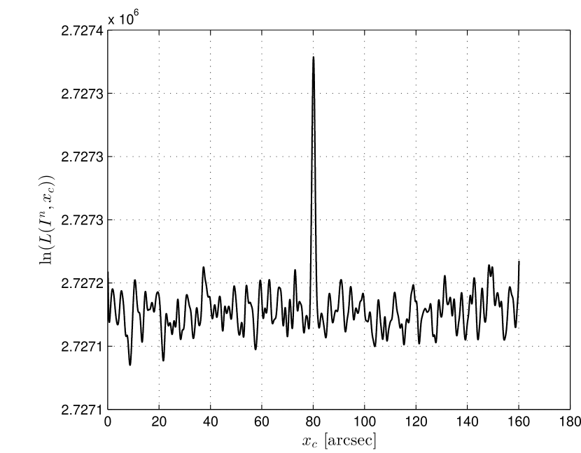
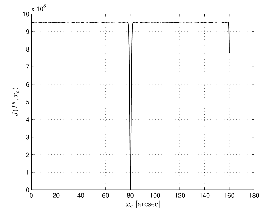
Figure 7: Example behavior of the likelihood function $\ln L(I^{n},x_{c})$ (upper row) and LS function $J(I^{n},x_{c})$ (lower row) for two particular realizations with low SNR= 12 (left column) and high SNR= 230 (right column), for a target centered at $x_{c}=80$ arcsec (for a pixel size of $\Delta x=0.2$ arcsec). All the other parameters are those described in Section 4. The figures show (particularly the ones at low SNR) the non-linear nature of both objective functions.

The solution to equation (16) is non-linear (see Figure 7), and it does not have a closed-form expression. Consequently, a number of iterative approaches have been adopted (see, e.g., Stetson (1987); Mighell (2005)) to solve or approximate $\tau_{LS}(I^{n})$. Hence as $\tau_{LS}(I^{n})$ is implicit, it is not possible to compute its mean, its variance, nor its estimation error directly. We also note that, since we will be mainly analyzing the behavior of $\tau_{LS}(I^{n})$, none of the caveats concerning the properness of the likelihood function (equation (5)) raised in Section 2.1 are relevant in what follows, except for what concerns the adequacy of equation (2), which we take as a valid description of the underlying flux distribution.

The problem of computing the MSE of an estimator that is the solution of an optimization problem has been recently addressed by So et al. (2013) using a general framework. Their basic idea was to provide sufficient conditions on the objective function, in our case $J(I^{n},\alpha)$, to derive a good approximation for $\mathbb{E}_{I^{n}\sim f_{x_{c}}}\left\{\left(\tau_{LS}(I^{n})-x_{c}\right)^{2}\right\}$. Based on this idea, we provide below a refined result (specialized to our astrometry problem), which relaxes one of the idealized assumptions proposed in So et al. (2013, their equation (5)), and which is not strictly satisfied in our problem (see Remark 2 in Section 3.3). As a consequence, our result offers upper and lower bounds for the bias and MSE of $\tau_{LS}(I^{n})$, respectively.

Theorem 1

Let us consider a fixed and unknown parameter $x_{c}\in\mathbb{R}$, and that $I^{n}\sim f_{x_{c}}$. In addition, let us define the residual random variable $W(I^{n},\alpha)\equiv\frac{J^{\prime\prime}(I^{n},\alpha)-\mathbb{E}_{I^{n}\sim f_{x_{c}}}\left\{J^{\prime\prime}(I^{n},\alpha)\right\}}{\mathbb{E}_{I^{n}\sim f_{x_{c}}}\left\{J^{\prime\prime}(I^{n},\alpha)\right\}}$. If there exists $\delta\in(0,1)$ such that $\mathbb{P}(W(I^{n},x_{c})\in(-\delta,\delta))=1$, then:

$$\left|\mathbb{E}_{I^{n}\sim f_{x_{c}}}\left\{\tau_{LS}(I^{n})\right\}-x_{c}\right|\leq\epsilon(\delta),$$ (17)

$$\mathbb{E}_{I^{n}\sim f_{x_{c}}}\left\{\left(\tau_{LS}(I^{n})-x_{c}\right)^{2}\right\}\in\left(\frac{\sigma^{2}_{LS}(n)}{(1+\delta)^{2}},\frac{\sigma^{2}_{LS}(n)}{(1-\delta)^{2}}\right),$$ (18)

where

$$\sigma^{2}_{LS}(n)\equiv\frac{\mathbb{E}_{I^{n}\sim f_{x_{c}}}\left\{J^{\prime}(I^{n},x_{c})^{2}\right\}}{\left(\mathbb{E}_{I^{n}\sim f_{x_{c}}}\left\{J^{\prime\prime}(I^{n},x_{c})\right\}\right)^{2}}$$ (19)

and

$$\epsilon(\delta)\equiv\frac{\mathbb{E}_{I^{n}\sim f_{x_{c}}}\left\{\left|J^{\prime}(I^{n},x_{c})\right|\right\}}{\mathbb{E}_{I^{n}\sim f_{x_{c}}}\left\{J^{\prime\prime}(I^{n},x_{c})\right\}}\cdot\frac{\delta}{1-\delta}.$$ (20)

(The proof is presented in Appendix B).

3.3 Analysis and interpretation of Theorem 1

Remark 1

Theorem 1 is obtained under a bounded condition (with probability one) over the random variable $W(I^{n},x_{c})$. To verify whether this condition is actually met, it is therefore important to derive an explicit expression for $W(I^{n},x_{c})$. Starting from equation (16) it follows that:

$$J^{\prime\prime}(I^{n},\alpha)=2\sum_{i=1}^{n}\left[\left(\frac{d\lambda_{i}(\alpha)}{d\alpha}\right)^{2}+(\lambda_{i}(\alpha)-I_{i})\cdot\frac{d^{2}\lambda_{i}(\alpha)}{d^{2}\alpha}\right]$$

and, consequently, $\mathbb{E}_{I^{n}\sim f_{x_{c}}}\left\{J^{\prime\prime}(I^{n},x_{c})\right\}=2\sum_{i=1}^{n}\left(\frac{d\lambda_{i}(\alpha)}{d\alpha}|_{\alpha=x_{c}}\right)^{2}$. Therefore:

$$W(I^{n},x_{c})=\sum_{i=1}^{n}(\lambda_{i}(x_{c})-I_{i})\cdot\left[\lambda_{i}^{\prime\prime}(x_{c})/\sum_{j=1}^{n}(\lambda_{j}^{\prime}(x_{c}))^{2}\right].$$ (21)

Then, $W(I^{n},x_{c})$ is not bounded almost surely, since $I_{i}$ could take any value in $\mathbb{N}$ with non-zero probability. However, $\mathbb{E}_{I^{n}\sim f_{x_{c}}}\left\{W(I^{n},x_{c})\right\}=0$, and its variance in closed-form is:

$$Var(W(I^{n},x_{c}))=\sum_{i=1}^{n}\lambda_{i}(x_{c})\cdot\left[(\lambda_{i}^{\prime\prime}(x_{c}))^{2}/\left(\sum_{j=1}^{n}(\lambda_{j}^{\prime}(x_{c}))^{2}\right)^{2}\right].$$ (22)

From this, we can evaluate how far we are from the bounded assumption of Theorem 1. To do this, we can resort to Markov’s inequality (Cover & Thomas, 2006), where $\mathbb{P}(W(I^{n},x_{c})\notin(-\rho,\rho))\leq Var(W(I^{n},x_{c}))/\rho^{2}$. Then, for any $\epsilon\in(0,1)$, we can characterize a critical $\delta(\epsilon)>0$ such that $\mathbb{P}(W(I^{n},x_{c})\in(-\delta(\epsilon),\delta(\epsilon)))>1-\epsilon$. Using this result and Theorem 1, we can bound the conditional bias and conditional MSE of $\tau_{LS}(I^{n})$ using equations (17) and (18), respectively. In Section 4, we conduct a numerical analysis, where it is shown that the bounded assumption for $W(I^{n},x_{c})$ is indeed satisfied for a number of important realistic experimental settings in astrometry (with very high probability).

Remark 2

Concerning the MSE of the LS estimator, equation (18) offers a lower and upper bound in terms of a nominal value $\sigma^{2}_{LS}(n)$ (given by equation (19)), and an interval around it. In the interesting regime where $\delta\ll 1$ (this regime approaches the ideal case $\delta=0$ studied by So et al. (2013) in which case the variable $W(I^{n},x_{c})$ becomes deterministic), we have that $\tau_{LS}(\cdot)$ is an unbiased estimator, as shown by equation (17), and, furthermore:

$$Var(\tau_{LS}(I^{n}))=\mathbb{E}_{I^{n}\sim f_{x_{c}}}\left\{\left(\tau_{LS}(I^{n})-x_{c}\right)^{2}\right\}=\sigma^{2}_{LS}(n)\geq\sigma_{CR}^{2},$$

from equations (18) and (10). Thus, it is interesting to provide an explicit expression for $\sigma^{2}_{LS}(n)$ which will be valid for the MSE of the LS method in this regime. First we note that, $J^{\prime}(I^{n},x_{c})=2\cdot\left(\sum_{i=1}^{n}\frac{d\lambda_{i}(x_{c})}{dx_{c}}\cdot(\lambda_{i}(x_{c})-I_{i})\right)$, and therefore:

$$(J^{\prime}(I^{n},x_{c}))^{2}= 4\cdot\left(\sum_{i=1}^{n}\sum_{j=1,j\neq i}^{n}(I_{i}I_{j}-I_{i}\lambda_{j}-I_{j}\lambda_{i}+\lambda_{i}\lambda_{j})\cdot\frac{d\lambda_{i}}{dx_{c}}\cdot\frac{d\lambda_{j}}{dx_{c}}\right)$$

$$+4\cdot\left(\sum_{i=1}^{n}(I_{i}^{2}-2I_{i}\lambda_{i}+\lambda_{i}^{2})\cdot\left(\frac{d\lambda_{i}}{dx_{c}}\right)^{2}\right).$$

Therefore $\mathbb{E}_{I^{n}\sim f_{x_{c}}}\left\{J^{\prime}(I^{n},x_{c})^{2}\right\}=4\cdot\sum_{i=1}^{n}\lambda_{i}(x_{c})\cdot(\lambda_{i}^{\prime}(x_{c}))^{2}$, which implies that:

$$\sigma^{2}_{LS}(n)=\frac{\sum_{i=1}^{n}\lambda_{i}(x_{c})\cdot(\lambda_{i}^{\prime}(x_{c}))^{2}}{\left(\sum_{i=1}^{n}(\lambda_{i}^{\prime}(x_{c}))^{2}\right)^{2}}=\frac{\sum_{i=1}^{n}(\tilde{F}g_{i}(x_{c})+\tilde{B}_{i})\cdot(g_{i}^{\prime}(x_{c}))^{2}}{\left(\tilde{F}\sum_{i=1}^{n}(g_{i}^{\prime}(x_{c}))^{2}\right)^{2}}.$$ (23)

In the next section, we provide a numerical analysis to compare the predictions of equation (23) with the CR bound computed through equation (12). We also analyze if this nominal value is representative of the performance of the LS estimator.

Remark 3

(Idealized Low SNR regime) Following the ideal scenario where $\delta\ll 1$, we explore the weak signal case in which $\tilde{F}g_{i}(x_{c})\ll\tilde{B}_{i}$ considering a constant background across the pixels, i.e., $\tilde{B}_{i}=\tilde{B}$ for all $i$. Then adopting equation (23) we have that:

$$\sigma^{2}_{LS}(n)\approx\frac{\tilde{B}}{\tilde{F}^{2}\sum_{i=1}^{n}(g_{i}^{\prime}(x_{c}))^{2}}.$$ (24)

On the other hand, from equation (12) we have that $\mathcal{I}_{x_{c}}(n)\approx{\tilde{F}^{2}}/{\tilde{B}}\sum_{i=1}^{n}(g_{i}^{\prime}(x_{c}))^{2}$. Remarkably in this context, the LS estimator is optimal in the sense that it approaches the CR bound asymptotically when a weak signal is observed. This results is consistent with the numerical simulations in Mendez et al. (2013, Table 3).

Remark 4

(Idealized High SNR regime) For the high SNR regime, assuming again that $\delta\ll 1$, we consider the case where $\tilde{F}g_{i}(x_{c})\gg\tilde{B}_{i}$ for all $i$. In this case:

$$\sigma^{2}_{LS}(n)\approx\left[\tilde{F}\frac{\left(\sum_{i=1}^{n}g_{i}^{\prime}(x_{c})^{2}\right)^{2}}{\sum_{i=1}^{n}g_{i}(x_{c})g_{i}^{\prime}(x_{c})^{2}}\right]^{-1}\mbox{ and }\sigma_{CR}^{2}\approx\left[\tilde{F}\sum_{i=1}^{n}(g_{i}^{\prime}(x_{c}))^{2}/g_{i}(x_{c})\right]^{-1}.$$ (25)

Therefore, in this strong signal scenario, there is no match between the variance of the LS estimator and the CR bound, and consequently, we have that $\sigma^{2}_{LS}(n)>\sigma_{CR}^{2}$. To provide more insight on the nature of this performance gap, in the next proposition we offer a closed-form expression for this mismatch in the high-resolution scenario where the source is oversampled, and the size of the pixel is a small fraction of the width parameter $\sigma$ of the PSF in equation (1).

Proposition 3

Assuming the idealized high SNR regime, if we have a Gaussian-like PSF and $\Delta x/\sigma\ll 1$, then:

$$\frac{\sigma^{2}_{LS}(n)}{\sigma_{CR}^{2}}\approx\frac{8}{3\sqrt{3}}>1.$$ (26)

(The proof is presented in Appendix C).

Equation (26) shows that there is a very significant performance gap between the CR bound and the MSE of the LS estimator in the high SNR regime. This result should motivate the exploration of alternative estimators that could approach more closely the CR bound in this regime.

4 Numerical analysis of the LS estimator

In this section we explore the implications of Theorem 1 in astrometry through the use of simulated observations. First, we analyze if the bounded condition over $W(I^{n},\alpha)$ adopted in Theorem 1 is a valid assumption for the type of settings considered in astronomical observations. After that, we compare how efficient is the LS estimator proposed in equation (16) as a function of the SNR and pixel resolution, adopting for that purpose Theorem 1 and Proposition 1.

To perform our simulations, we adopt some realistic design variables and astronomical observing conditions to model the problem (Mendez et al., 2013, 2014). For the PSF, various analytical and semi-empirical forms have been proposed, see for instance the ground-based model in King (1971) and the space-based model in Bendinelli et al. (1987). For our analysis, we adopt in equation (3) the Gaussian PSF where $\phi(x,\sigma)=\frac{1}{\sqrt{2\pi}\,\sigma}e^{-\frac{1}{2}\cdot\left(\frac{x}{\sigma}\right)^{2}}$, and where $\sigma$ is the width of the PSF, assumed to be known. This PSF has been found to be a good representation for typical astrometric-quality ground-based data (Mendez et al., 2010). In terms of nomenclature, the $FWHM\equiv 2\sqrt{2\ln 2}\,\,\sigma$, measured in arcsec, denotes the Full-Width at Half-Maximum ($FWHM$) parameter, which is an overall indicator of the image quality at the observing site (Chromey, 2010).

The background profile, represented by $\left\{\tilde{B}_{i},i=1,..,n\right\}$, is a function of several variables, like the wavelength of the observations, the moon phase (which contributes significantly to the diffuse sky background), the quality of the observing site, and the specifications of the instrument itself. We will consider a uniform background across pixels underneath the PSF, i.e., $\tilde{B_{i}}=\tilde{B}$ for all $i$. To characterize the magnitude of $\tilde{B}$, it is important to first mention that the detector does not measure photon counts (or, actually, photo-$e^{-}$) directly, but a discrete variable in “Analog to Digital Units (ADUs)” of the instrument, which is a linear proportion of the photon counts (Gilliland, 1992). This linear proportion is characterized by the gain of the instrument $G$ in units of $e^{-}$/ADU. $G$ is just a scaling factor, where we can define $F\equiv\tilde{F}/G$ and $B\equiv\tilde{B}/G$ as the brightness of the object and background, respectively, in the specific ADUs of the instrument. Then, the background (in ADUs) depends on the pixel size $\Delta x$ as follows (Mendez et al., 2013):

$$B=f_{s}\cdot\Delta x+\frac{D+RON^{2}}{G}\;\;\mbox{ADU},$$ (27)

where $f_{s}$ is the (diffuse) sky background in ADU/arcsec (if $\Delta x$ is measured in arcsec), while $D$ and $RON$, both measured in $e^{-}$, model the dark-current and read-out-noise of the detector on each pixel, respectively. Note that the first component in equation (27) is attributed to the site, and its effect is proportional to the pixel size. On the other hand, the second component is attributed to errors of the integrating device (detector), and it is pixel-size independent. This distinction is central when analyzing the performance as a function of the pixel resolution of the array (see details in Mendez et al. (2013, Sec. 4)). More important is the fact that in typical ground-based astronomical observation, long exposure times are considered, which implies that the background is dominated by diffuse light coming from the sky (the first term in the RHS of equation (27)), and not from the detector (Mendez et al., 2013, Sec. 4).

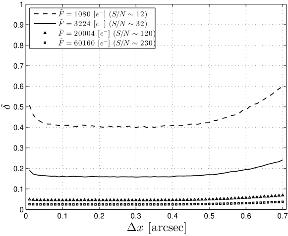
Figure 2: Numerical computation of the critical $\delta$ (dimensionless) such that $P(W(I^{n},x_{c})\in(-\delta,\delta))>1-10^{-3}$. In all the scenarios (SNR, and $\Delta x$), $5\,000$ realizations of the random variable $W(I^{n},x_{c})$ are used to estimate the probability distribution for $W(I^{n},x_{c})$, and $\delta$, from frequency counts. As $\delta$ decreases, we have a smaller bias (see equations (17) and (20)) and a narrower range for the MSE of the LS estimator (equation (18)).

For the experimental conditions, we consider the scenario of a ground-based station located at a good site with clear atmospheric conditions and the specifications of current science-grade CCDs, where $f_{s}=1502.5$ ADU/arcsec, $D=0$ $e^{-}$, $RON=5$ $e^{-}$, $FWHM=1$ arcsec and $G=2$ $e^{-}$/ADU (with these values $B=313$ ADU for $\Delta x=0.2$ arcsec using equation (27)). In terms of scenarios of analysis, we explore different pixel resolutions for the CCD array $\Delta x\in[0.1,0.7]$ measured in arcsec. Note that a change in $\Delta x$ will be reflected upon the limits of the integral to compute the pixel response function $g_{i}(x_{c})$ (see equation (3)) as well as in the calculation of the background level per pixel $\tilde{B}_{i}$, according to equation (27). Therefore, a change in $\Delta x$ is not only a design feature of the detector device, but it implies also a change in the distribution of the background underneath the PSF. The impact of this covariant device-and-atmosphere change in the CR bound is explained in detail in Mendez et al. (2013, Section 4, see also their Figure 2).

In our simulations, we also consider different signal strengths $\tilde{F}\in\left\{1\,080,3\,224,20\,004,60\,160\right\}$, measured in photo-$e^{-}$, corresponding to SNR $\in\sim\left\{12,33,120,230\right\}$ respectively. Note that increasing $\tilde{F}$ implies increasing the SNR of the problem, which can be approximately measured by the ratio $\tilde{F}/\tilde{B}\equiv F/B$. On a given detector plus telescope setting, these different SNR scenarios can be obtained by changing appropriately the exposure time (open shutter) that generates the image.

4.1 Analyzing the bounded condition over $W(I^{n},\alpha)$

To validate how realistic is the bounded assumption over $W(I^{n},\alpha)$ in our problem, we first evaluate the variance of $W(I^{n},x_{c})$ from equation (22), this is presented in Figure 1 for different SNR regimes and pixel resolutions in the array. Overall, the magnitudes are very small considering the admissible range $(0,1)$ for $W(I^{n},x_{c})$ stipulated in Theorem 1. Also, given that $W(I^{n},x_{c})$ has zero mean, the bounded condition will happen with high probability. Complementing this, Figure 2 presents the critical $\delta$ across different pixel resolutions and SNR regimes. For this, we fix a small value of $\epsilon$ ($=10^{-3}$ in this case), and calculate $\delta$ such that $W(I^{n},x_{c})\in(-\delta,\delta)$ with probability $1-\epsilon$. From the curves obtained, we can say that the bounded assumption is holding (values of $\delta$ in $(0,1)$) for a wide range of representative experimental conditions and, consequently, we can use Theorem 1 to provide a range on the performance of the LS estimator. Note that the idealized condition of $\delta\approx 0$ is realized only for the very high SNR regime (strong signals).

4.2 Performance Analysis of the LS estimator

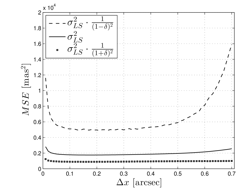
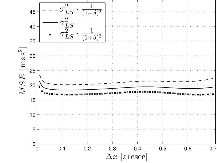
Figure 3: Range of the MSE performance (in milli-arcsec² = mas²) for the LS method in astrometry predicted by Theorem 1 (equations (18) and (19)). Results are reported for different representative values of $\tilde{F}$ and across different pixel sizes: (From top-left to bottom-right) $\tilde{F}=1\,080$ e^-; $\tilde{F}=3\,224$ e^-; $\tilde{F}=20\,004$ e^-; $\tilde{F}=60\,160$ e^-.

We adopt equation (18) which provides an admissible range for the MSE performance of the LS estimator. For that we use the critical $\delta$ obtained in Figure 2. These curves for the different SNR regimes and pixel resolutions are shown in Figure 3. Following the trend reported in Figure 2, the nominal value $\sigma_{LS}^{2}$ is a precise indicator for the LS estimator performance for strong signals (matching the idealized conditions stated in Remark 4), while on the other hand, Theorem 1 does not indicate whether $\sigma_{LS}^{2}$ is accurate or not for low SNR, as we deviate from the idealized case elaborated in Remark 3. Nevertheless, we will see, based on some complementary empirical results reported in what follows, that even for low SNR, the nominal $\sigma_{LS}^{2}$ predicts the performance of the LS estimator quite well.

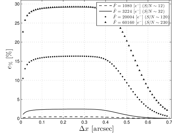
Figure 4: Relative performance differences between $\sigma_{LS}^{2}$ in Theorem 1 (equation (19)) and the CR bound $\sigma_{CR}^{2}$ in Proposition 1 (equation (12)). Results are reported for different SNR and pixel sizes. A significant performance gap between the LS technique and the CR bound is found for $FWHM$/$\Delta x<1$ (good sampling of the PSF) at high SNR, indicating that, in this regime, the LS method is sub-optimal, in agreement with Proposition 3 (see also equation (26)). This gap becomes monotonically smaller as the SNR decreases.

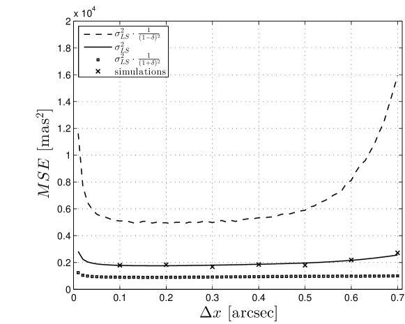
Figure 6: Comparison between the nominal value $\sigma_{LS}^{2}$, the performance range $\left(\frac{\sigma_{LS}^{2}(n)}{(1+\delta)^{2}},\frac{\sigma_{LS}^{2}(n)}{(1-\delta)^{2}}\right)$ stipulated in Theorem 1, and the empirical estimation of $\mathbb{E}_{I^{n}\sim f_{x_{c}}}\{\left(\tau_{LS}(I^{n})-x_{c}\right)^{2}\}$ from simulations for a low SNR regime of $\tilde{F}=1\,080$ e^-. The fact that the simulations follow closely the nominal value, even at low SNR, justifies the use of $\sigma_{LS}$ as given by equations (19) and (23) as a benchmark of the LS method at any SNR.

Assuming for a moment the idealized case in which $\delta\ll 1$, we can reduce the performance analysis to measuring the gap between the nominal value predicted by Theorem 1 (equation (19)), and the CR bound in Proposition 1. Figure 4 shows the relative difference given by $e_{\%}=\frac{\sigma_{LS}^{2}-\sigma_{CR}^{2}}{\sigma_{CR}^{2}}\cdot 100$. From the figure we can clearly see that, in the low SNR regime, the relative performance differences tends to zero and, consequently, the LS estimator approaches the CR bound, and it is therefore an efficient estimator. This matches what has been stated in Remark 3. On the other hand for high SNR, we observe a performance gap that is non negligible (up to $\approx 27\%$ relative difference above the CR for $\tilde{F}=60\,160$ $e^{-}$, and $\approx 15\%$ above the CR for $\tilde{F}=20\,004$ $e^{-}$ for $\Delta x=0.2$ arcsec). This is consistent with what has been argued in Remark 4. Note that in this regime, the idealized scenario in which $\delta\ll 1$ is valid (see Figure 2) and, thus, $\mathbb{E}_{I^{n}\sim f_{x_{c}}}\left\{\left(\tau_{LS}(I^{n})-x_{c}\right)^{2}\right\}\approx\sigma_{LS}^{2}$, which is not strictly the case for the low SNR regime (although see Figure 6, and the discussion that follows).

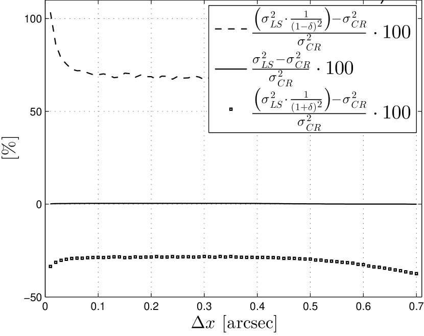
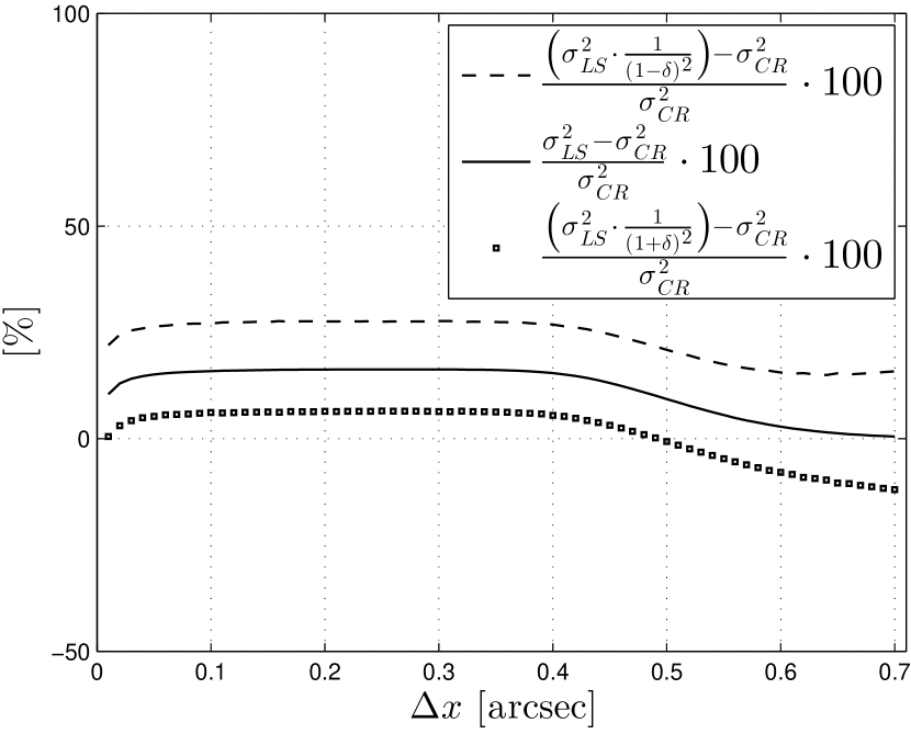
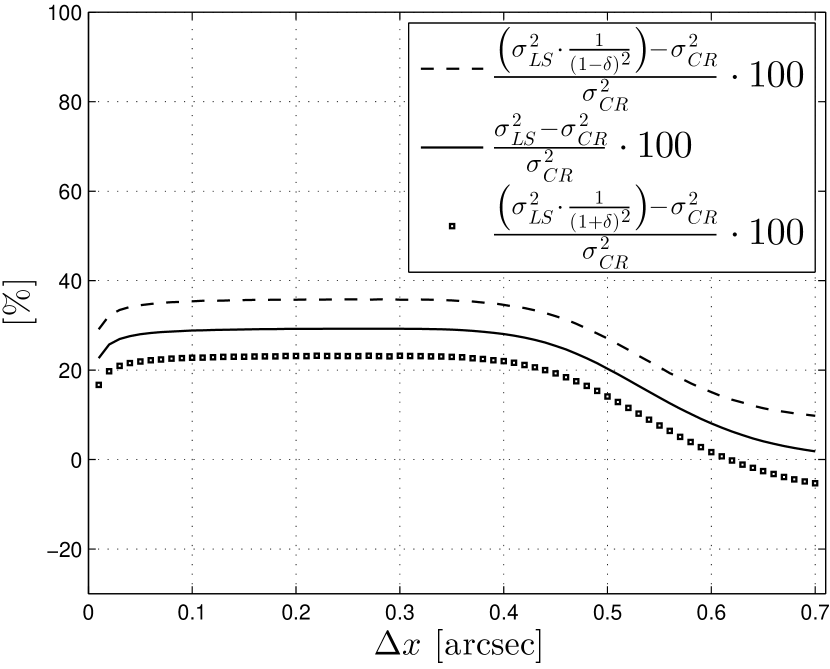
Figure 5: Relative performance differences between the range of performance $\left(\frac{\sigma_{LS}^{2}(n)}{(1+\delta)^{2}},\frac{\sigma_{LS}^{2}(n)}{(1-\delta)^{2}}\right)$ stipulated in Theorem 1 for the LS estimator (equations (18) and (19)) and the CR bound $\sigma_{CR}^{2}$ in Proposition 1 (equation (12)). Results are reported for different $\tilde{F}$ and across different pixel sizes: (From top-left to bottom-right) $\tilde{F}=1\,080$ e^-; $\tilde{F}=3\,224$ e^-; $\tilde{F}=20\,004$ e^-; $\tilde{F}=60\,160$ e^-. The 0% level corresponds to having achieved the CR bound. Note that as the SNR decreases, the bias (see equations (17) and (20), and the possible range for the MSE of the LS method (see equations (18)) increase (see also Figure 2).

To refine the relative performance analysis presented in Figure 4, Figure 5 shows the feasible range (predicted by Theorem 1) of performance gap considering the critical $\delta$ obtained in Figure 2. We report four cases, from very low to very high SNR regimes, to illustrate the trends. From this figure, we can see that the deviations from the nominal value are quite significant for the low SNR regime, and that, from this perspective, the range obtained from Theorem 1 is not sufficiently small to conclude about the goodness of the LS estimator in this context. On the other hand, in the high SNR regime, the nominal comparison can be considered quite precise.

The results of the previous paragraph motivate an empirical analysis to estimate the performance of the LS estimator empirically from the data, with the goal of resolving the low SNR regime illustrated in Figure 5. For this purpose, $1\,000$ realizations were considered for all the SNR regimes and pixel sizes, and the performance of the LS estimator was computed using the empirical MSE. We used a large number of samples to guarantee convergence to the true MSE error as a consequence of the law of large numbers (Gray & Davisson, 2010). Remarkably, we observe in all cases that the estimated performance matches quite tightly the nominal $\sigma_{LS}^{2}$ characterized by Theorem 1. We illustrate this in Figure 6, which considers the most critical low SNR regime. Consequently, from this numerical analysis, we can resolve the ambiguity present in the low SNR regime, and conclude that the comparison with the nominal result reported in Figure 4, and the derived conclusion about the LS estimator in the low and high SNR regimes, can be considered valid. Our simulations also show that the LS estimator is unbiased. Overall, these results suggests that Theorem 1 could be improved, perhaps by imposing milder sufficient conditions, in order to prove that $\sigma_{LS}^{2}$ is indeed a precise indicator of the MSE of the LS estimator at any SNR regime.

For completeness, we show in Figure 7 the behavior of the log-likelihood function (computed using equation (13)) and the LS function $J(I^{n},x_{c})$ (computed using equation (16)) for our two extreme SNR cases of our numerical simulations, namely SNR= 12 and SNR= 230. In these figures the true astrometric position is at $x_{c}=80$ arcsec (= 400 pix with $\Delta x$ = 0.2 arcsec). These figures clearly show (particularly the one at low SNR) the non-linear nature of both objective functions.

5 Summary and Final Remarks

Our work provides results to characterize the performance of the widely used LS estimator as applied to the problem of astrometry when derived from digital discrete array detectors. The main result (Theorem 1) provides in closed-form a nominal value ($\sigma^{2}_{LS}(n)$), and a range around it, for the MSE of the LS estimator as well as its bias. From the predicted nominal value, we analyzed how efficient is the LS estimator in comparison with the MV CR bound. In particular, we show that the LS estimator is efficient in the regime of low SNR (a point source with a weak signal), in the sense that it approximates very closely the CR bound. On the other hand, we show that at high SNR there is a significant gap in the performance of the LS estimator with respect to the MV bound. We believe that this sub-optimal behavior is caused by the Poissonian nature of the detection process, in which the variance per pixel increases as the signal itself. Since the LS method is very sensitive to outliers, the large excursions caused by the large pixel intensity variance at high SNR make the LS method less efficient (from the point of view of its MSE), than allowed by the CR bound. These performance analyses complement and match what has been observed in photometric estimation, where only in the low SNR regime the LS estimator has been shown to asymptotically achieve the CR bound.

While our results are valid for an idealized linear (one-dimensional) array detector where intra-pixel response changes are neglected, and where flat-fielding is achieved with very high accuracy, our findings should motivate the exploration of alternative estimators in the high SNR observational regime. Regarding this last point, we note that an inspection of Mendez et al. (2013, Table 3) suggests that either a (Poisson variance-) weighted LS or a ML approach do not exhibit this loss of optimality at high-SNR, and should be preferred to the unweighted LS analyzed in this paper. This effect is clearly illustrated in Figure 8, where we present a comparison between the standard deviation of the LS and ML methods derived from numerical simulations in the very high SNR regime (where the gap between CR and the LS is most significant). Motivated by these results, a detailed analysis of the ML method will be presented in a forthcoming paper.

6 Acknowledgments

We are indebted to an anonymous referee that read the draft carefully and in great detail, providing us with several suggestions and comments that have improved the legibility of the text significantly. In particular his/her suggestions have lead to the introduction of Figures 7, 8 and the corresponding discussion in the body of the paper.

This material is based on work supported by a grant from CONICYT-Chile, Fondecyt # 1151213. In addition, the work of J. F. Silva and M. Orchard is supported by the Advanced Center for Electrical and Electronic Engineering, Basal Project FB0008. J. F. Silva acknowledges support from a CONICYT-Fondecyt grant # 1140840 , and R. A. Mendez acknowledges support from Project IC120009 Millennium Institute of Astrophysics (MAS) of the Iniciativa Científica Milenio del Ministerio de Economía, Fomento y Turismo de Chile. R.A.M also acknowledges ESO/Chile for hosting him during his sabbatical-leave during 2014.

Appendix A Proof of Proposition 2

We use the well-known fact that the CR bound is achieved by an unbiased estimator, if and only if, the following decomposition holds (Kendall et al., 1999, pp. 12)

$$\frac{d\ln L(I^{n};\theta)}{d\theta}=A(\theta,n)\cdot(f(I^{n})-\theta),$$ (A1)

where $L(I^{n};\theta)$ is the likelihood of the observation $I^{n}\in\mathbb{N}^{n}$ given $\theta$, $A(\theta,n)$ is a function of $\theta$ and $n$ alone (i.e., it does dot depend on the data), while $f(I^{n})$ is a function of the data exclusively (i.e., it does not depend on the parameter). Furthermore, if the achievability condition in equation (A1) is satisfied, then $A(\theta,n)=\mathcal{I}_{\theta}(n)$, and $f(I^{n})$ is an unbiased estimator of $\theta$ that achieves the CR bound.

The proof follows by contradiction, assuming that equation (A1) holds. First using equation (5), we have that:

$$\frac{d\ln L(I^{n};x_{c})}{dx_{c}}=\sum_{i=1}^{n}\left[\frac{I_{i}}{\lambda_{i}(x_{c})}\cdot\frac{d\lambda_{i}(x_{c})}{dx_{c}}-\frac{d\lambda_{i}(x_{c})}{dx_{c}}\right]=\sum_{i=1}^{n}\frac{I_{i}}{\lambda_{i}(x_{c})}\cdot\frac{d\lambda_{i}(x_{c})}{dx_{c}},$$ (A2)

the last equality comes from the fact that $\sum_{i=1}^{n}g_{i}(x_{c})=1$ from the assumption in equation (4). Then replacing equations (A2) and (12) in equation (A1):

$$f(I^{n})=\sum_{i=1}^{n}\frac{\frac{I_{i}}{\tilde{F}g_{i}(x_{c})+\tilde{B}_{i}}\cdot\frac{dg_{i}(x_{c})}{dx_{c}}}{\tilde{F}\sum_{i=1}^{n}\frac{1}{\tilde{F}g_{i}(x_{c})+\tilde{B}_{i}}\cdot\left(\frac{dg_{i}(x_{c})}{dx_{c}}\right)^{2}}+x_{c},$$ (A3)

which contradicts the assumption that $f(I^{n})$ should be a function of the data alone. Furthermore, if we consider the extreme high SNR regime, where $\tilde{F}g_{i}(x_{c})\gg\tilde{B}_{i}$ for all $i$, and the low SNR regime, where $\tilde{F}g_{i}(x_{c})\ll\tilde{B}_{i}$ for all $i$, it follows that:

$$f(I^{n})=\sum_{i=1}^{n}I_{i}\cdot\frac{d\ln g_{i}(x_{c})}{dx_{c}}\cdot\left[\tilde{F}\sum_{i=1}^{n}\left(\frac{dg_{i}(x_{c})}{dx_{c}}\right)^{2}/g_{i}(x_{c})\right]^{-1}+x_{c}$$ (A4)

and

$$f(I^{n})=\sum_{i=1}^{n}\frac{I_{i}}{\tilde{B}_{i}}\cdot\frac{dg_{i}(x_{c})}{dx_{c}}\cdot\left[\tilde{F}\sum_{i=1}^{n}\left(\frac{dg_{i}(x_{c})}{dx_{c}}\right)^{2}/\tilde{B}_{i}\right]^{-1}+x_{c},$$ (A5)

respectively. Therefore a contradiction remains even in these extreme SNR regimes.

Appendix B Proof of Theorem 1

The approach of So et al. (2013) uses the fact that the objective function $J(I^{n},\alpha)$ in equation (16) is two times differentiable, which is satisfied in our context. As a short-hand, if we denote by $\hat{x}_{c}$ the LS estimator solution $\tau_{LS}(I^{n})$, then the first order necessary condition for a local optimum requires that $J^{\prime}(I^{n},\hat{x}_{c})\equiv\frac{dJ(I^{n},\alpha)}{d\alpha}|_{\alpha=\hat{x}_{c}}=0$. The other key assumption in So et al. (2013) is that $\hat{x}_{c}$ is in a close neighborhood of the true value $x_{c}$. In our case, this has to do with the quality of the pixel-based data used for the inference, which we assume it offers a good estimation of the position (see, e.g., King (1983); Stone (1989)). Then using a first order Taylor expansion of $J^{\prime}(I^{n},\hat{x}_{c})$ around $x_{c}$, the following key approximation can be adopted (So et al., 2013, their equation (4)):

$$0=J^{\prime}(I^{n},\hat{x}_{c})=J^{\prime}(I^{n},x_{c})+(\hat{x}_{c}-x_{c})\cdot J^{\prime\prime}(I^{n},x_{c})\Leftrightarrow(x_{c}-\hat{x}_{c})=\frac{J^{\prime}(I^{n},x_{c})}{J^{\prime\prime}(I^{n},x_{c})},$$ (B1)

where $J^{\prime\prime}(I^{n},x_{c})\equiv\frac{d^{2}J(I^{n},\alpha)}{d^{2}\alpha}|_{\alpha=x_{c}}$. If we consider $I^{n}\sim f_{x_{c}}$, then from equation (B1):

$$x_{c}-\tau_{LS}(I^{n})=\frac{J^{\prime}(I^{n},x_{c})}{J^{\prime\prime}(I^{n},x_{c})}.$$ (B2)

The second step in the approximation proposed by So et al. (2013) is to bound $\frac{J^{\prime}(I^{n},x_{c})}{J^{\prime\prime}(I^{n},x_{c})}$ by $\frac{J^{\prime}(I^{n},x_{c})}{\mathbb{E}_{I^{n}\sim f_{x_{c}}}\left\{J^{\prime\prime}(I^{n},x_{c})\right\}}$. For that we introduce the residual variable $W(I^{n},\alpha)$ where $J^{\prime\prime}(I^{n},x_{c})=\mathbb{E}_{I^{n}\sim f_{x_{c}}}\left\{J^{\prime\prime}(I^{n},x_{c})\right\}(1+W(I^{n},x_{c}))$. Using the fact that $W(I^{n},\alpha)$ is bounded almost surely (see Remark 1, and Section 4.1):

$$\left|\frac{J^{\prime}(I^{n},x_{c})}{\mathbb{E}_{I^{n}\sim f_{x_{c}}}\left\{J^{\prime\prime}(I^{n},x_{c})\right\}}-\frac{J^{\prime}(I^{n},x_{c})}{J^{\prime\prime}(I^{n},x_{c})}\right| = \left|\frac{J^{\prime}(I^{n},x_{c})}{\mathbb{E}_{I^{n}\sim f_{x_{c}}}\left\{J^{\prime\prime}(I^{n},x_{c})\right\}}\cdot\left[1-\frac{1}{1+W(I^{n},x_{c})}\right]\right|$$ (B3)

$$\leq \left|\frac{J^{\prime}(I^{n},x_{c})}{\mathbb{E}_{I^{n}\sim f_{x_{c}}}\left\{J^{\prime\prime}(I^{n},x_{c})\right\}}\right|\cdot\max_{w\in(-\delta,\delta)}\left|1-\frac{1}{1+w}\right|$$

$$\leq \frac{\left|J^{\prime}(I^{n},x_{c})\right|}{\mathbb{E}_{I^{n}\sim f_{x_{c}}}\left\{J^{\prime\prime}(I^{n},x_{c})\right\}}\cdot\frac{\delta}{1-\delta},$$

the last step uses the fact that $\mathbb{E}_{I^{n}\sim f_{x_{c}}}\left\{J^{\prime\prime}(I^{n},x_{c})\right\}\geq 0$ (see Remark 1). On the other hand, Jensen’s inequality (Cover & Thomas, 2006) guarantees that:

$$\left|\frac{\mathbb{E}_{I^{n}\sim f_{x_{c}}}\left\{J^{\prime}(I^{n},x_{c})\right\}}{\mathbb{E}_{I^{n}\sim f_{x_{c}}}\left\{J^{\prime\prime}(I^{n},x_{c})\right\}}-\mathbb{E}_{I^{n}\sim f_{x_{c}}}\left\{\frac{J^{\prime}(I^{n},x_{c})}{J^{\prime\prime}(I^{n},x_{c})}\right\}\right| \leq \mathbb{E}_{I^{n}\sim f_{x_{c}}}\left\{\left|\frac{J^{\prime}(I^{n},x_{c})}{\mathbb{E}_{I^{n}\sim f_{x_{c}}}\left\{J^{\prime\prime}(I^{n},x_{c})\right\}}-\frac{J^{\prime}(I^{n},x_{c})}{J^{\prime\prime}(I^{n},x_{c})}\right|\right\}$$ (B4)

$$\leq \frac{\mathbb{E}_{I^{n}\sim f_{x_{c}}}\left\{\left|J^{\prime}(I^{n},x_{c})\right|\right\}}{\mathbb{E}_{I^{n}\sim f_{x_{c}}}\left\{J^{\prime\prime}(I^{n},x_{c})\right\}}\cdot\frac{\delta}{1-\delta},$$

where the last inequality comes from equation (B3). Then we use that $J^{\prime}(I^{n},x_{c})=2\cdot\sum_{i=1}^{n}(\lambda_{i}(x_{c})-I_{i})\cdot\frac{d\lambda_{i}(x_{c})}{dx_{c}}$, and consequently $\mathbb{E}_{I^{n}\sim f_{x_{c}}}\left\{J^{\prime}(I^{n},x_{c})\right\}=0$. Then from equations (B4) and (B2), we have that:

$$\left|x_{c}-\mathbb{E}_{I^{n}\sim f_{x_{c}}}\left\{\tau_{LS}(I^{n})\right\}\right|\leq\frac{\mathbb{E}_{I^{n}\sim f_{x_{c}}}\left\{\left|J^{\prime}(I^{n},x_{c})\right|\right\}}{\mathbb{E}_{I^{n}\sim f_{x_{c}}}\left\{J^{\prime\prime}(I^{n},x_{c})\right\}}\cdot\frac{\delta}{1-\delta},$$ (B5)

which leads to equation (17).

Concerning the MSE, from the hypothesis on $W(I^{n},x_{c})$ we have that:

$$\frac{J^{\prime}(I^{n},x_{c})^{2}}{\mathbb{E}_{I^{n}\sim f_{x_{c}}}\left\{J^{\prime\prime}(I^{n},x_{c})\right\}^{2}(1+\delta)^{2}}\leq\left(\frac{J^{\prime}(I^{n},x_{c})}{J^{\prime\prime}(I^{n},x_{c})}\right)^{2}\leq\frac{J^{\prime}(I^{n},x_{c})^{2}}{\mathbb{E}_{I^{n}\sim f_{x_{c}}}\left\{J^{\prime\prime}(I^{n},x_{c})\right\}^{2}(1-\delta)^{2}},$$ (B6)

almost surely. Then taking the expected value in equation (B6) and using equation (B2) for the central term, it follows that:

$$\frac{\mathbb{E}_{I^{n}\sim f_{x_{c}}}\left\{J^{\prime}(I^{n},x_{c})^{2}\right\}}{\mathbb{E}_{I^{n}\sim f_{x_{c}}}\left\{J^{\prime\prime}(I^{n},x_{c})\right\}^{2}(1+\delta)^{2}}\leq\mathbb{E}_{I^{n}\sim f_{x_{c}}}\left\{\left(x_{c}-\tau_{LS}(I^{n})\right)^{2}\right\}\\ \leq\frac{\mathbb{E}_{I^{n}\sim f_{x_{c}}}\left\{J^{\prime}(I^{n},x_{c})^{2}\right\}}{\mathbb{E}_{I^{n}\sim f_{x_{c}}}\left\{J^{\prime\prime}(I^{n},x_{c})\right\}^{2}(1-\delta)^{2}},$$

which concludes the result.

Appendix C Proof of Proposition 3

Recalling from equation (3) that $g_{i}(x_{c})=\int_{x_{i}-\frac{\Delta x}{2}}^{x_{i}+\frac{\Delta x}{2}}\phi(x-x_{c},\sigma)\,dx$ and assuming a Gaussian PSF of the form $\phi(x,\sigma)=\frac{1}{\sqrt{2\pi}\,\sigma}\exp{\left(\frac{-x^{2}}{2\sigma^{2}}\right)}$ (see Section 4) by the mean value theorem and the hypothesis of small pixel ($\Delta x/\sigma\ll 1$), it is possible to state that:

$$g_{i}(x_{c})\approx\phi(x_{i}-x_{c},\sigma)\cdot\Delta x,$$ (C1)

and then we have that:

$$\frac{dg_{i}(x_{c})}{dx_{c}} \approx \frac{(x_{i}-x_{c})}{\sigma^{2}}\cdot\frac{1}{\sqrt{2\pi}\,\sigma}\exp\left(\frac{-(x_{i}-x_{c})^{2}}{2\sigma^{2}}\right)\cdot\Delta x$$ (C2)

$$= \frac{(x_{i}-x_{c})}{\sigma^{2}}\cdot\phi(x_{i}-x_{c},\sigma)\cdot\Delta x.$$

With the above approximation we have that:

$$\sum_{i=1}^{n}\left(\frac{dg_{i}(x_{c})}{dx_{c}}\right)^{2}g_{i}(x_{c}) \approx \sum_{i=1}^{n}\left(\frac{(x_{i}-x_{c})}{\sigma^{2}}\cdot\phi(x_{i}-x_{c},\sigma)\cdot\Delta x\right)^{2}\cdot\phi(x_{i}-x_{c},\sigma)\cdot\Delta x$$ (C3)

$$\approx \frac{\Delta x^{2}}{2\sqrt{3}\pi\sigma^{6}}\cdot\sum_{i=1}^{n}(x_{i}-x_{c})^{2}\frac{1}{\sqrt{2\pi}\frac{\sigma}{\sqrt{3}}}\exp\left(\frac{-(x_{i}-x_{c})^{2}}{2\left(\frac{\sigma}{\sqrt{3}}\right)^{2}}\right)\cdot\Delta x.$$

The term inside the summation in equation (C3) can be approximated by an integral due to the small-pixel hypothesis. Assuming that the source is well sampled by the detector (see Section 2.1, equation (4)) we can obtain that:

$$\sum_{i=1}^{n}\left(\frac{dg_{i}(x_{c})}{dx_{c}}\right)^{2}g_{i}(x_{c}) \approx \frac{\Delta x^{2}}{2\sqrt{3}\pi\sigma^{6}}\int_{-\infty}^{+\infty}(x-x_{c})^{2}\frac{1}{\sqrt{2\pi}\frac{\sigma}{\sqrt{3}}}\exp\left(\frac{-(x-x_{c})^{2}}{2\left(\frac{\sigma}{\sqrt{3}}\right)^{2}}\right)dx$$ (C4)

$$= \frac{\Delta x^{2}}{2\sqrt{3}\pi\sigma^{6}}\cdot\frac{\sigma^{2}}{3}=\frac{\Delta x^{2}}{6\sqrt{3}\pi\sigma^{4}},$$ (C5)

where equation (C5) follows from the fact that the term inside the integral in equation (C4) corresponds to the second moment of a normal random variable of mean $x_{c}$ and variance $\frac{\sigma^{2}}{3}$.

By the same set of arguments used to approximate $\sum_{i=1}^{n}\left(\frac{dg_{i}(x_{c})}{dx_{c}}\right)^{2}g_{i}(x_{c})$ in equation (C5), we have that:

$$\sum_{i=1}^{n}\left(\frac{dg_{i}(x_{c})}{dx_{c}}\right)^{2} \approx \sum_{i=1}^{n}\left(\frac{(x_{i}-x_{c})}{\sigma^{2}}\cdot\phi(x_{i}-x_{c},\sigma)\cdot\Delta x\right)^{2}$$ (C6)

$$\approx \frac{\Delta x}{2\sqrt{\pi}\sigma^{5}}\cdot\sum_{i=1}^{n}(x_{i}-x_{c})^{2}\frac{1}{\sqrt{2\pi}\frac{\sigma}{\sqrt{2}}}\exp\left(\frac{-(x_{i}-x_{c})^{2}}{2\left(\frac{\sigma}{\sqrt{2}}\right)^{2}}\right)\cdot\Delta x$$

$$\approx \frac{\Delta x}{2\sqrt{\pi}\sigma^{5}}\int_{-\infty}^{+\infty}(x-x_{c})^{2}\frac{1}{\sqrt{2\pi}\frac{\sigma}{\sqrt{2}}}\exp\left(\frac{-(x-x_{c})^{2}}{2\left(\frac{\sigma}{\sqrt{2}}\right)^{2}}\right)dx$$

$$\approx \frac{\Delta x}{2\sqrt{\pi}\sigma^{5}}\cdot\frac{\sigma^{2}}{2}=\frac{\Delta x}{4\sqrt{\pi}\sigma^{3}},$$ (C7)

where equation (C7) follows from the fact that the term inside the integral in equation (C6) is the second moment of a normal random variable of mean $x_{c}$ and variance $\frac{\sigma^{2}}{\sqrt{2}}$.

Finally, for $\sum_{i=1}^{n}\left(\frac{dg_{i}(x_{c})}{dx_{c}}\right)^{2}\cdot\frac{1}{g_{i}(x_{c})}$ we proceed again in the same way, namely:

$$\sum_{i=1}^{n}\left(\frac{dg_{i}(x_{c})}{dx_{c}}\right)^{2}\frac{1}{g_{i}(x_{c})} \approx \sum_{i=1}^{n}\left(\frac{(x_{i}-x_{c})}{\sigma^{2}}\cdot\phi(x_{i}-x_{c},\sigma)\cdot\Delta x\right)^{2}\frac{1}{\phi(x_{i}-x_{c},\sigma)\cdot\Delta x}$$ (C8)

$$\approx \frac{1}{\sigma^{4}}\sum_{i=1}^{n}(x_{i}-x_{c})^{2}\frac{1}{\sqrt{2\pi}\sigma}\exp\left(\frac{-(x_{i}-x_{c})^{2}}{2\sigma^{2}}\right)\Delta x$$

$$\approx \frac{1}{\sigma^{4}}\int_{-\infty}^{+\infty}\frac{(x-x_{c})^{2}}{\sqrt{2\pi}\sigma}\exp\left(\frac{-(x-x_{c})^{2}}{2\sigma^{2}}\right)dx$$

$$\approx \frac{1}{\sigma^{4}}\cdot\sigma^{2}=\frac{1}{\sigma^{2}},$$ (C9)

where equation (C9) follows from the fact that the term inside the integral in equation (C8) corresponds to the second moment of a normal random variable of mean $x_{c}$ and variance $\sigma^{2}$.

Then adopting equations (C5), (C7) and (C9) in equations (23) and (12), respectively, and assuming a uniform background underneath the PSF, we have that:

$$\sigma_{LS}^{2} = \frac{\sum_{i=1}^{n}\left(\frac{dg_{i}(x_{c})}{dx_{c}}\right)^{2}g_{i}(x_{c})}{\tilde{F}\left(\sum_{i=1}^{n}\left(\frac{dg_{i}(x_{c})}{dx_{c}}\right)^{2}\right)^{2}}+\frac{\tilde{B}}{\tilde{F}^{2}\sum_{i=1}^{n}\left(\frac{dg_{i}(x_{c})}{dx_{c}}\right)^{2}}$$ (C10)

$$\approx \frac{\frac{\Delta x^{2}}{6\sqrt{3}\pi\sigma^{4}}}{\tilde{F}\left(\frac{\Delta x}{4\sqrt{\pi}\sigma^{3}}\right)^{2}}+\frac{\tilde{B}}{\tilde{F}^{2}\frac{\Delta x}{4\sqrt{\pi}\sigma^{3}}}$$

$$= \frac{\sigma^{2}}{\tilde{F}}\left[\frac{8}{3\sqrt{3}}+4\sqrt{\pi}\frac{1}{\frac{\Delta x}{\sigma}}\frac{\tilde{B}}{\tilde{F}}\right]\approx\frac{\sigma^{2}}{\tilde{F}}\frac{8}{3\sqrt{3}}$$

and,

$$\sigma_{CR}^{2}=\frac{1}{\sum_{i=1}^{n}\frac{\left(\tilde{F}\frac{dg_{i}(x_{c})}{dx_{c}}\right)^{2}}{\tilde{F}g_{i}(x_{c})+\tilde{B}}}=\frac{1}{\tilde{F}\sum_{i=1}^{n}\left(\frac{dg_{i}(x_{c})}{dx_{c}}\right)^{2}\frac{1}{g_{i}(x_{c})}}\approx\frac{\sigma^{2}}{\tilde{F}}.$$ (C11)

In the last step in equation (C10) and the last step in equation (C11), we have used the assumption that $\tilde{F}\gg\tilde{B}$. We note that the last step in equation (C11) corresponds to the second line of equation (45) in Mendez et al. (2013).

Figure 1: Variance of the residual random variable $W(I^{n},x_{c})$ (dimensionless) as given by equation (22), as a function of the pixel resolution $\Delta x$ arcsec for different realistic SNR scenarios (function of $\tilde{F}$) encountered in ground-based astronomical observations. Since the admissible range for $\delta$ is the interval (0,1), the small computed values indicates that the bounded assumption in Theorem 1 can be considered as valid under these conditions.

Figure 8: Comparison of the $\sqrt{MSE}$ derived from numerical simulations using the ML (open circles, equation (13)) and the LS method (open squares, equation (16)) for a high SNR= 230 (see, e.g., right column of Figure 7), where the optimality loss (performance gap, $\sim$15% in this case) of the LS method (Proposition 3) in this regime is clearly seen. The solid line is the nominal $\sigma_{LS}(n)$ derived from our theorem (equation (19)), while the dashed line is the CR limit, $\sigma_{CR}$, given by equation (12). As we have shown (Section (3.1)), the CR limit can not be reached in our astrometric setting, but our ML simulations (open circles) show that they can follow very closely this limit (see also Mendez et al. (2013, Table 3)). A detailed analytical study of the optimality of the ML method will be presented in a forthcoming paper.

References

- Adorf (1996) Adorf, H.-M. 1996, in Astronomical Data Analysis Software and Systems V, Vol. 101, 13
- Alard & Lupton (1998) Alard, C., & Lupton, R. H. 1998, AJ, 503, 325
- Auer & van Altena (1978) Auer, L., & van Altena, W. 1978, AJ, 83, 531
- Bastian (2004) Bastian, U. 2004. GAIA technical note, GAIA-C3-TN-ARI-BAS-020 (http://www.cosmos.esa.int/web/gaia/public-dpac-documents). Available at http://www.rssd.esa.int/SYS/docs/ll_transfers/project=PUBDB&id=2939027.pdf (last accessed on April 2015).
- Becker et al. (2007) Becker, A. C., Silvestri, N. M., Owen, R. E., Ivezić, Ž., & Lupton, R. H. 2007, PASP, 119, 1462
- Bendinelli et al. (1987) Bendinelli, O., Parmeggiani, G., Piccioni, A., & Zavatti, F. 1987, AJ, 94, 1095
- Cameron et al. (2006) Cameron, A. C., et al. 2006, MNRAS, 373, 799
- Chromey (2010) Chromey, F. R. 2010, To measure the sky: an introduction to observational astronomy (Cambridge University Press)
- Cover & Thomas (2006) Cover, T. M., & Thomas, J. A. 2006, Elements of Information Theory (second ed.) (Wiley Interscience, New York)
- Cramér (1946) Cramér, H. 1946, Scandinavian Actuarial Journal, 1946, 85
- Fessler (1996) Fessler, J. A. 1996, Image Processing, IEEE Transactions on, 5, 493
- Gawiser et al. (2006) Gawiser, E., van Dokkum, P. G., Herrera, D., et al. 2006, ApJS, 162, 1
- Gilliland (1992) Gilliland, R. L. 1992, in Astronomical Society of the Pacific Conference Series, Vol. 23, Astronomical CCD Observing and Reduction Techniques, ed. S. B. Howell, 68
- Freyhammer et al. (2001) Freyhammer, L. M., Andersen, M. I., Arentoft, T., Sterken, C., & Nørregaard, P. 2001, Experimental Astronomy, 12, 147
- Gray & Davisson (2010) Gray, R. M., & Davisson, L. D. 2010, An Introduction to Statistical Signal Processing, Cambridge University Press
- Høg (2009) Høg, E. 2009, Experimental Astronomy, 25, 225
- Høg (2011) Høg, E. 2011, Baltic Astronomy, 20, 221
- Honeycutt (1992) Honeycutt, R. K. 1992, PASP, 435
- Howell (2006) Howell, S. B. 2006, Handbook of CCD astronomy, Vol. 5 (Cambridge University Press)
- Jakobsen et al. (1992) Jakobsen, P., Greenfield, P., & Jedrzejewski, R. 1992, A&A, 253, 329
- Kay (1993) Kay, S. M. 1993, Fundamentals of Statistical Signal Processing, Volume I: Estimation Theory. Prentice Hall, New Jersey.
- Kendall et al. (1999) Kendall, M., Stuart, A., Ord, J., & Arnold, S. 1999, Vol. 2A: Classical inference and the linear model (London [etc.]: Arnold [etc.])
- King (1971) King, I. R. 1971, PASP, 199
- King (1983) King, I. R. 1983, PASP, 163
- Lattanzi (2012) Lattanzi, M. 2012, Mem. Soc. Astron. Italiana, 83, 1033
- Lee & van Altena (1983) Lee, J.-F., & van Altena, W. 1983, AJ, 88, 1683
- Lindegren (1978) Lindegren, L. 1978, in IAU Colloq. 48: Modern Astrometry, Vol. 1, 197
- Lindegren (2000) Lindegren, L. 2000, Gaia technical report Gaia-LL-032
- Lindegren (2010) Lindegren, L. 2010, ISSI Scientific Reports Series, 9, 279
- Lupton et al. (2001) Lupton, R., Gunn, J. E., Ivezić, Z., Knapp, G. R., & Kent, S. 2001, Astronomical Data Analysis Software and Systems X, 238, 269
- Lupton (2007) Lupton, R. 2007, Statistical Challenges in Modern Astronomy IV, 371, 160
- Mason (2007) Mason, E. 2008, in The 2007 ESO Instrument Calibration Workshop, Kaufer, A., & Kerber, F. (eds.), Springer-Verlag, Berlin, 107
- Mendez et al. (2010) Mendez, R. A., Costa, E., Pedreros, M. H., Moyano, M., Altmann, M., & Gallart, C. 2010, PASP, 122, 853
- Mendez et al. (2013) Mendez, R. A., Silva, J. F., & Lobos, R. 2013, PASP, 125, pp. 580
- Mendez et al. (2014) Mendez, R. A., Silva, J. F., Orostica, R., & Lobos, R. 2014, PASP, 126, 798
- Mighell (2005) Mighell, K. J. 2005, MNRAS, 361, 861
- Najim (2008) Najim, M. 2008, Modeling, Estimation and Optimal Filtering in Signal Processing, Chapter A, 335-340. Available at http://onlinelibrary.wiley.com/book/10.1002/9780470611104, last accessed on June 26th, 2015.
- Perryman et al. (1989) Perryman, M., Jakobsen, P., Colina, L., Lelievre, G., Macchetto, F., Nieto, J., & Serego Alighieri, S. 1989, A&A, 215, 195
- Pier et al. (2003) Pier, J. R., Munn, J. A., Hindsley, R. B., et al. 2003, AJ, 125, 1559
- Rao (1945) Rao, C. R. 1945, Bulletin of the Calcutta Mathematical Society, 37, 81
- Raykar et al. (2005) Raykar, V. C., Kozintsev, I. V., & Lienhart, R. 2005, Speech and Audio Processing, IEEE Transactions on, 13, 70
- Reffert (2009) Reffert, S. 2009, New A Rev., 53, 329
- So et al. (2013) So, H., Chan, Y., Ho, K., & Chen, Y. 2013, Signal Processing Magazine, IEEE, 30, 162
- Stetson (1987) Stetson, P. B. 1987, PASP, 191
- Stone (1989) Stone, R. C. 1989, AJ, 97, 1227
- Tyson (1986) Tyson, J. A. 1986, Journal of the Optical Society of America A, 3, 2131
- van Altena & Auer (1975) van Altena, W., & Auer, L. 1975, in Image Processing Techniques in Astronomy (Springer), 411
- van Altena (2013) van Altena, W. F. 2013, Astrometry for Astrophysics: Methods, Models, and Applications (Cambridge University Press)
- Winick (1986) Winick, K. A. 1986, J. Opt. Soc. Am. A, 3, 1809
- Zaccheo et al. (1995) Zaccheo, T., Gonsalves, R., Ebstein, S., & Nisenson, P. 1995, ApJ, 439, L43