Bridges in the random-cluster model

Abstract

The random-cluster model, a correlated bond percolation model, unifies a range of important models of statistical mechanics in one description, including independent bond percolation, the Potts model and uniform spanning trees. By introducing a classification of edges based on their relevance to the connectivity we study the stability of clusters in this model. We prove several exact relations for general graphs that allow us to derive unambiguously the finite-size scaling behavior of the density of bridges and non-bridges. For percolation, we are also able to characterize the point for which clusters become maximally fragile and show that it is connected to the concept of the bridge load. Combining our exact treatment with further results from conformal field theory, we uncover a surprising behavior of the (normalized) variance of the number of (non-)bridges, showing that it diverges in two dimensions below the value $4\cos^{2}{(\pi/\sqrt{3})}=0.2315891\cdots$ of the cluster coupling $q$. Finally, we show that a partial or complete pruning of bridges from clusters enables estimates of the backbone fractal dimension that are much less encumbered by finite-size corrections than more conventional approaches.

1 Introduction

Percolation is probably the most widely discussed and arguably the simplest model of critical phenomena. Due to a combination of conceptual simplicity and wide applicability which is a signature of a problem of very general interest, its many incarnations including bond and site percolation on a lattice as well as continuum and non-equilibrium, directed variants, have been the subject of thousands of studies [1]. In statistical physics and mathematics alike, the quest to understand aspects of the percolation problem has led to developments of powerful and beautiful new techniques [2, 3]. While the problem is well defined and interesting for any graph or lattice, both finite and infinite, the understanding of non-trivial cases is most advanced in two dimensions. There, the scaling limit of critical percolation can be related to the Coulomb gas [4] and conformal field theory [5], leading to exact results for most critical exponents and certain correlation functions. More recently, a rigorous approach to conformal field theory was pioneered by Schramm who used a mapping introduced by Löwner to construct a way of generating conformally invariant fractal random curves, the Stochastic (or Schramm) Löwner Evolutions (SLEs) [6], for which a range of properties, including fractal dimensions, can be calculated exactly. In this context, Smirnov and co-workers used the concept of discrete analyticity to establish rigorously that the scaling limits of critical percolation [7, 8] and the Ising model [9] on the triangular lattice are indeed conformally invariant, and cluster boundaries in these models converge to certain classes of SLE traces.

The random-cluster (RC) model was suggested by Fortuin and Kasteleyn as a natural extension of the (bond) percolation problem, noting that there was a class of models fulfilling the series and parallel laws of electrical circuits that also included the Ising model [10]. Given a graph $G=(V,E)$, it assigns to a spanning subgraph $(V,A\subseteq E)$ a probability mass (in the following also referred to as RC measure) [11]

$$\mathbb{P}_{p,q,G}[A]=\frac{p^{|A|}(1-p)^{|E|-|A|}q^{K(A)}}{Z_{\rm RC}(p,q,G)},\quad A\in\Omega_{G},$$ (1.1)

where $K(A)$ is the number of components and $|A|$ the number of edges in $A$. The quantity $Z_{\mathrm{RC}}(p,q,G)$ is the partition function of the RC model, corresponding to the sum of unnormalized weights, and $\Omega_{G}$ constitutes the set of all spanning subgraphs or configurations, i.e., $\Omega_{G}=\{A:A\subseteq E\}$. Edges that are in $A$ are called open and those in $E\setminus A$ closed. The presence of the cluster-weight factor $q^{K(A)}$ distinguishes (1.1) from the percolation problem and prevents $\mathbb{P}_{p,q,G}[A]$ from being a Bernoulli product measure; only for $q\to 1$, where the model reduces to the percolation problem and hence edges become independent, this property is restored. Although the cluster weight $q$ can be any non-negative real number, integer values of $q$ are particular in that for them the partition function is very closely related to that of the $q$-state Potts model [12] (see Eq. (2.3) below). For lattice graphs in at least two dimensions, the model undergoes a percolation phase transition at a critical value $p_{c}(q)$ of the bond probability where, for sufficiently large $q$ the transition becomes discontinuous [11]. On the square lattice, self-duality allows to deduce the exact transition point $p_{\mathrm{c}}(q)=p_{\mathrm{sd}}(q)=\sqrt{q}/(1+\sqrt{q})$ [13], and the location of the tricritical point is known to be $q_{\mathrm{c}}=4$, beyond which the transition becomes of first order [14].

The crucial importance of the RC description for the understanding of critical phenomena is through its expression in purely geometrical terms. Hence understanding the geometric structure of the (correlated) percolation problem (1.1) provides a geometric route to the understanding of the thermal phase transition of the Potts model. Correspondingly, significant effort has been devoted in particular to investigations of the structure of the incipient percolating cluster. While initially it was assumed that it was a network of nodes connected by essentially one-dimensional links, results regarding the conductivity of the critical cluster implied that, instead, the structure is better described by the more elaborate ‘links–nodes–blobs’ picture [15]. If one fixes two distant points $A$ and $B$ on the cluster, those bonds that have independent, non-intersecting paths to both $A$ and $B$ form the backbone of the cluster. It is essentially the part that would carry current in case a voltage was applied between $A$ and $B$. The remaining cluster mass is in dangling ends. The backbone itself consists of singly-connected or red bonds that destroy percolation or, equivalently, destroy conductivity between $A$ and $B$ if cut (the links which meet in the nodes) as well as bonds in cycles that are multiply connected (the blobs). These subsets of bonds have fractal scaling with associated exponents $d_{\mathrm{F}}$ for the cluster mass itself, $d_{\mathrm{BB}}$ for the backbone, and $d_{\mathrm{RB}}$ for the red bonds. Obviously one has $d_{\mathrm{RB}}\leq d_{\mathrm{BB}}\leq d_{\mathrm{F}}$, and it turns out that strict inequality holds in the generic case and hence asymptotically almost all of the bonds of the incipient percolating cluster are in dangling ends, and almost all of the mass of the backbone is in the blobs. In two dimensions, exact expressions for $d_{\mathrm{F}}$ and $d_{\mathrm{RB}}$ are available from Coulomb gas arguments [16], but $d_{\mathrm{BB}}$ is only known numerically [17, 18].

As we discuss here, the distinction of singly-connected and multiply-connected bonds first suggested for understanding the backbone structure [15] is a more generally useful classification of bonds in a cluster configuration. Removing singly connected bonds, which we call bridges, generates an additional connected component, while this is not the case for multiply connected bonds or non-bridges. Indeed, this separation allows us to control the effect of a local edge manipulation (open $\leftrightarrow$ closed) on the weight of the configuration as in Eq. (1.1). We will exploit this below to derive expressions for the expected number of bridges and related classes of bonds as well as the scale of fluctuations in the former. A further partitioning of bridges was recently suggested for percolation in Ref. [18]: branches are bridges for which at least one of the connected clusters is a tree, whereas the remaining bridges are dubbed junctions. This distinction is related to but not congruent with the links–nodes–blobs picture: most of the red bonds will be junctions, but so are some bonds in dangling ends as well. Cutting the branches, on the other hand, will remove some part of the dangling ends (the treelike ones), and branches are not typically found in the backbone. As a result of this incongruence, the number of junctions on the percolating cluster grows as $L^{d_{\mathrm{F}}}$ and not proportional to $L^{d_{\mathrm{RB}}}$, where $L$ is the linear size of the system. In contrast to the class of red bonds, therefore, both branches and junctions are extensive subsets of the bridges. For uncorrelated percolation Xu et al. [18] find numerically, however, that removing all bridges, i.e., both branches and junctions, leads to tightly connected remainders, corresponding to the blobs, whose size grows as $L^{d_{\mathrm{BB}}}$. As we will show below in Sec. 6, it suffices to remove the junctions only to see the same behavior more generally for the RC model.

As, by definition, the removal of a bridge leads to the generation of a new component and hence the breakup of an existing cluster, understanding the properties of bridge bonds is crucial also to the understanding of fragmentation phenomena in the framework of a lattice model. This connection was investigated in our recent letter [20], where we studied the fragmentation rate and kernel, and related the associated scaling exponents to the more standard critical exponents and fractal dimensions. In the present paper, however, we follow a different line of study. In particular, we derive a linear relation between the expected density of bridges and the density of bonds; we provide the asymptotic densities of bridges in the thermodynamic limit for the square lattice and study the scaling corrections in finite systems in general. We employ Monte Carlo simulations based on the Swendsen-Wang–Chayes-Machta algorithm [21, 22] and a recent new implementation [23] of Sweeny’s algorithm [24] to confirm these results for the square lattice and study the behavior in three dimensions. Building on these results for the densities, i.e., the first moment of the bridge distribution, we move on to studying the fluctuations, corresponding to the second moment. We reveal an unexpected finite-size behavior leading to a non-specific-heat variance singularity for $q\leq 4\cos{(\pi/\sqrt{3})}^{2}$, a direct consequence of an intriguing interplay between bridges and non-bridges.

The rest of this paper is organized as follows. In Section 2 we introduce the edge classification, derive the bridge-edge identity in general, consider some of its consequences and present a numerical study for the special case of the square lattice, together with a detailed analysis of finite-size corrections. In Section 3 we use symmetries of the RC model in order to derive connections to other quantities of interest in the percolation literature, such as the short range connectivity. In Section 4 we introduce the concept of bridge load which allows us to analytically characterize the point of maximal bridge density for independent bond percolation. In Section 5 we derive a second-order bridge-edge identity that allows us to study the variance of the number of bridges. In Section 6 we compare various new and old methods to extract the backbone fractal dimension, with an emphasis on the involved finite-size corrections. Section 7 contains our conclusions.

2 Bridge density

2.1 Edwards-Sokal coupling

Although in this paper we focus on the RC model itself, its relation to the Potts model is of relevance for the physical interpretation of the (geometric) percolation transition in terms of a thermal phase transition. In particular, we make reference to how certain observables of the Potts model translate into quantities in the RC language. The Potts model describes interacting spins, and assigns one of the $q$ spin values in $\{1,\ldots,q\}$ to each vertex, attributing a configurational probability or Boltzmann weight

$$\mathbb{P}_{\beta,q,G}[\boldsymbol{\sigma}]\equiv\frac{1}{Z_{\mathrm{P}}(\beta,q,G)}\sum_{\boldsymbol{\sigma}\in\mathcal{Q}}\exp{\left(\beta\sum_{(x,y)\in E}\mathds{1}_{\{\sigma_{x}=\sigma_{y}\}}\right)}=\frac{1}{Z_{\mathrm{P}}(\beta,q,G)}\prod_{(x,y)\in E}e^{\beta}[1-p+p\mathds{1}_{\{\sigma_{x}=\sigma_{y}\}}],$$ (2.1)

to a spin configuration $\boldsymbol{\sigma}=\{\sigma_{1},\ldots,\sigma_{|V|}\}\in\mathcal{Q}=\{1,\cdots,q\}^{|V|}$. Here, we write $\mathds{1}_{\{\sigma_{x}=\sigma_{y}\}}$ for the indicator function, which equals $1$ if $\sigma_{x}=\sigma_{y}$ and $0$ otherwise. Analogous to $Z_{\mathrm{RC}}(p,q,G)$, the Potts partition function $Z_{\mathrm{P}}(\beta,q,G)$ corresponds to the sum of the unnormalized weights. Importantly, in the second equality, we need to identify $p=1-e^{-\beta}$. The relation between Eqs. (1.1) and (2.1) is established by augmenting phase space to include both, spin variables $\boldsymbol{\sigma}$ and subgraph variables $A$, leading to the joint probability

$$\mathbb{P}_{p,q,G}[\boldsymbol{\sigma},A]\equiv\frac{1}{Z_{\mathrm{joint}}(p,q,G)}\prod_{(x,y)\in E}e^{\beta}[(1-p)\mathds{1}_{\{e\notin A\}}+p\mathds{1}_{\{\sigma_{x}=\sigma_{y}\}}\mathds{1}_{\{e\in A\}}],$$ (2.2)

that is also known as Edwards-Sokal coupling [25]. It has the crucial property that the marginal distribution on the spins alone reduces to the Potts weight (2.1), while the marginal on the subgraphs gives the RC weight (1.1). Similarly, one can derive the conditional probabilities for the spins given the bonds or vice versa [11]. As was already shown by Fortuin and Kasteleyn [10], the corresponding partition functions coincide up to a (trivial) multiplicative factor if we relate the parameters $\beta$ and $p$ via $p=1-e^{-\beta}$,

$$Z_{\rm RC}{\left(1-e^{-\beta},q,G\right)}=e^{-\beta|E|}Z_{\rm P}(\beta,q,G)~{}\textnormal{for}~{}q\in\{2,3,\cdots\}.$$ (2.3)

This coupling is the basis for the Swendsen-Wang cluster algorithm [21] and its generalization to non-integer $q$ due to Chayes and Machta [22]. The above coupling and the identity (2.3) allow in particular to relate expectation values in the two ensembles. For instance, the internal energy in the Potts model is up to constants identical to the expected number of edges in the RC language,

$$u_{\beta,q,G}\equiv-\frac{1}{|V|}\frac{\partial\ln Z_{\mathrm{P}}(\beta,q,G)}{\partial\beta}=-\frac{1}{p}\frac{|E|}{|V|}\mathbb{E}_{p,q,G}[\mathcal{N}],~{}\textnormal{for}~{}p=1-e^{-\beta},$$ (2.4)

where ${\cal N}(A)=|A|/|E|$ is the proportion of open edges and $\mathbb{E}_{p,q,G}[\cdot]$ denotes the expectation with respect to the RC measure (1.1). Similarly, higher moments of the energy distribution such as the specific heat as well as magnetic observables of the Potts model can be expressed in terms of expectation values in the RC language [11]. Due to the conditional measures, correlation functions can also be related. Consider, in particular, the event $x\stackrel{{\scriptstyle A}}{{\leftrightarrow}}y$, that is the existence of a path in $A$ connecting $x$ and $y$. From the conditional measures derived from Eq. (2.2) it is easy to see that

$$\mathbb{E}_{p,q,G}[1-\mathds{1}_{\{\sigma_{x}=\sigma_{y}\}}|A]=\frac{q-1}{q}\left[1-\mathds{1}_{\left\{x\stackrel{{\scriptstyle A}}{{\leftrightarrow}}y\right\}}\right].$$ (2.5)

That is two vertices can only have unequal spin when they are not connected in the bond configuration and were assigned two different (random) colors. Summing over the edges shows that the nearest-neighbor connectivity defined as the sum

$${\cal E}(A)\equiv\frac{1}{|E|}\sum_{(x,y)\in E}\mathds{1}_{\left\{x\stackrel{{\scriptstyle A}}{{\leftrightarrow}}y\right\}}$$ (2.6)

is essentially the energy [26, 11, 27]

$$u_{\beta,q,G}=\frac{|E|}{|V|}-\frac{q-1}{q}\left(\frac{|E|}{|V|}-\mathbb{E}_{p,q,G}[\mathcal{E}]\right)~{}\textnormal{for}~{}p=1-e^{-\beta}.$$

Clearly for hypercubic lattices $|E|/|V|$ is bounded (more precisely equals $d$, where $d$ is the dimensionality).

2.2 Edge classification

Intuitively, (1.1) indicates that for $q>1$ $(q<1)$ the model favors configurations with a larger (smaller) number of components, compared to the case $q=1$. In this paper we investigate how the cluster structure is influenced by the cluster weight $q$, in particular with respect to the fragility of clusters. The relevance of individual edges for the connectivity of $A\subseteq E$ depends on whether they are pivotal or non-pivotal. According to our definition, pivotal edges change the number of components upon removal/insertion, i.e., for a pivotal edge $e$ we have $K(A^{e})=K(A_{e})-1$, where $A^{e}$ ($A_{e}$) is the configuration obtained from $A$ by opening (closing) $e$ (note that necessarily one of $A^{e}$ and $A_{e}$ is equal to $A$). Hence for a pivotal edge there is no alternative path connecting the vertices incident to it. As discussed above, for the purposes of this paper open pivotal edges are denoted as bridges, while we call pivotal closed edges candidate-bridges. Likewise, we denote open (closed) non-pivotal edges as non-bridges (candidate-non-bridges). Let $B$, $C$, $\overline{B}$, $\overline{C}$ denote the set of bridges, non-bridges, candidate-bridges and candidate-non-bridges, respectively. We stress that these sets depend explicitly on the configuration $A$. We denote the corresponding densities as ${\cal B}=|B|/|E|$, ${\cal C}=|C|/|E|$, $\overline{\cal B}=|\overline{B}|/|E|$, and $\overline{{\cal C}}=|\overline{C}|/|E|$.

2.3 Derivation of the bridge-edge formula

In this sub-section we show how, for arbitrary (finite) graphs, the expected densities of all the above mentioned edge-types $B$, $C$, $\overline{B}$, and $\overline{C}$ can be related to the expectation of the edge density. We establish these identities by utilizing a differential equation known as Russo-Margulis formula [28, 29], which applies to expectations with respect to product measures such as the probability density of the bond percolation model, corresponding to the $q=1$ RC model. The formula intuitively quantifies the “response” to an infinitesimal change in the bond density. Using this approach to quantify the response in the number of connected components $K$ allows us to study the bridge density. We then proceed and apply the idea to the RC model with generic $q>0$, by exploiting the fact that the partition function of the model can be interpreted as a particular expectation in the percolation model.

First consider the percolation model, i.e., the measure (1.1) with $q=1$, for which we denote expectations as $\mathbb{E}_{p,G}[\cdot]$. In this setting, the Russo-Margulis formula reads

$$\frac{\mathrm{d}}{\mathrm{d}p}\mathbb{E}_{p,G}[X]=\sum_{e\in E}\mathbb{E}_{p,G}[\delta_{e}X],$$ (2.7)

where $X(A):\Omega\rightarrow\mathbb{R}$ is an arbitrary observable and the quantity $\delta_{e}X$ is called the influence of $e$ on $X$ (or the discrete $e$-derivative of $X$) and is given by

$$(\delta_{e}X)(A)\equiv X(A^{e})-X(A_{e}).$$

The graph specific geometric properties of the model under study are “encoded” in the influences. In order to simplify the subsequent analysis, we show in Appendix A the following bijection identity:

$$\mathbb{E}_{p,G}[\delta_{e}X]=\frac{1}{p}\sum_{A\subseteq E:\atop e\in A}\mathbb{P}_{p,G}[A]\left[X(A)-X(A_{e})\right].$$ (2.8)

We now apply this identity to the cluster-number observable $K$, for which $K(A)-K(A_{e})=-1$ if $e$ is a bridge, $e\in B(A)$, and $0$ otherwise. Application of the Russo-Margulis formula (2.7) and Eq. (2.8) to $X=K$ then yields

$$\frac{\mathrm{d}}{\mathrm{d}p}\mathbb{E}_{p,G}[K]=\sum_{e\in E}\mathbb{E}_{p,G}[\delta_{e}K]=\frac{1}{p}\sum_{e\in E}\sum_{A\subseteq E:\atop e\in A}\mathbb{P}_{p,G}[A]\left[K(A)-K(A_{e})\right]=-\frac{1}{p}\sum_{e\in E}\mathbb{P}_{p,G}[e\in B]=-\frac{|E|}{p}\mathbb{E}_{p,G}[\mathcal{B}].$$ (2.9)

This differential equation allows us to determine the cluster numbers $\mathbb{E}_{p,G}[K]$ once the $p$-dependence of $\mathbb{E}_{p,G}[\mathcal{B}]$ is known. We remark that this relation was derived before in [30], however with a different target application in mind. As already mentioned, we can extend the above to the RC model and obtain more generally the bridge density $\mathbb{E}_{p,q,G}[\mathcal{B}]$ of the RC model itself. To start with, we note that the RC model partition function is $Z_{\rm RC}(p,q,G)=\mathbb{E}_{p,G}[q^{K}]$. In other words, the RC model partition function is the expected value of $q^{K}$ in the bond percolation model with parameter $p$. Hence we can apply the Russo-Margulis formalism to $q^{K}$. Using the same reasoning as that for $\mathbb{E}_{p,G}[K]$ above, we show in Appendix B that

$$\frac{\partial}{\partial p}\log{Z_{\rm RC}(p,q,G)}=|E|\frac{1-q}{p}\mathbb{E}_{p,q,G}[\mathcal{B}].$$ (2.10)

On the other hand, direct differentiation of the partition function $Z_{\mathrm{RC}}(p,q,G)$ yields

$$\frac{\partial}{\partial p}\log{Z_{\rm RC}(p,q,G)}=\frac{|E|}{1-p}\left(\frac{1}{p}\mathbb{E}_{p,q,G}[\mathcal{N}]-1\right).$$ (2.11)

Comparing both expressions (2.10) and (2.11), we derive the following relationship for the RC model (referred to as bridge-edge formula),

$$\mathbb{E}_{p,q,G}[\mathcal{B}]=\frac{\mathbb{E}_{p,q,G}[\mathcal{N}]-p}{(1-p)(1-q)},$$ (2.12)

which is of central importance for the following analysis (see [31] for some related identities developed along different lines). We remark again that this holds for any graph and for any $p\in(0,1)$ and $q\in(0,\infty)\setminus 1$ (the cases $q\rightarrow 0$, $1$ are discussed below). Due to the obvious identity $\mathbb{E}_{p,q,G}[\mathcal{N}]=\mathbb{E}_{p,q,G}[\mathcal{B}]+\mathbb{E}_{p,q,G}[\mathcal{C}]$, one immediately arrives at an analogous equation for the density of non-bridges,

$$\mathbb{E}_{p,q,G}[\mathcal{C}]=\frac{(pq-p-q)\mathbb{E}_{p,q,G}[\mathcal{N}]-p}{(1-p)(1-q)}.$$ (2.13)

We remark that in principle one can use the Russo-Margulis formalism to study the (partial) $p$-derivative of expectations of other observables in the RC model:

$$\frac{\partial}{\partial p}\mathbb{E}_{p,q,G}[X]=\frac{\partial}{\partial p}\left(\frac{\mathbb{E}_{p,G}[q^{K}X]}{\mathbb{E}_{p,G}[q^{K}]}\right)=\frac{\frac{\partial}{\partial p}\mathbb{E}_{p,G}[q^{K}X]}{\mathbb{E}_{p,G}[q^{K}]}+\frac{q-1}{p}\mathbb{E}_{p,q,G}[X]\mathbb{E}_{p,q,G}[|B|],$$

which shows the relevance of bridges in general for the RC model. Furthermore, let us consider a few direct consequences and applications of (2.12):

1. Firstly, notice that (2.12) recovers the correct results for the limit of uniform spanning trees, where all open edges are bridges. This tree model can be obtained in the RC model in the limit $q,p\rightarrow 0$ for $q/p\rightarrow 0$, which for the square lattice includes the critical line $p_{\rm sd}(q)$ [11].

2. It is possible to establish an upper bound for $\mathbb{E}_{p,q,G}[\mathcal{B}]$ for $q\geq 1$ and any $p$ on any graph. Using general comparison inequalities for the RC measure [32], it is possible to show that

   $$\mathbb{E}_{p,q,G}[\mathcal{N}]\geq\mathbb{E}_{\tilde{p}(p,q),1,G}[\mathcal{N}]=\frac{p}{(1-p)q+p}\equiv\tilde{p}(p,q),$$

   where $\tilde{p}(p,q)\leq p$ for $q\geq 1$. Together with (2.12) this yields the desired upper bound for $\mathbb{E}_{p,q,G}[\mathcal{B}]$

   $$\mathbb{E}_{p,q,G}[\mathcal{B}]=\frac{p-\mathbb{E}_{p,q,G}[\mathcal{N}]}{(1-p)(q-1)}\leq\frac{p-\tilde{p}(p,q)}{(1-p)(q-1)}=\tilde{p}(p,q).$$

   As is shown below for the Ising case $q=2$ with an exact solution this bound is tight in the limit $p\to 0$, but clearly not so for $p\gtrsim p_{\mathrm{sd}}$.

3. Another interesting consequence follows when one recasts (2.12) to express the edge density in terms of the bridge density

   $$\mathbb{E}_{p,q,G}[\mathcal{N}]=p-(q-1)(1-p)\mathbb{E}_{p,q,G}[\mathcal{B}].$$ (2.14)

   This emphasizes the importance of bridges for $q\neq 1$ as the source of finite-size corrections in $\mathbb{E}_{p,q,G}[\mathcal{N}]$, a manifestation of the introduction of correlations (deviation from the product measure). Moreover it also explains, in the setting of the RC model, how thermal fluctuations in the number of edges vanish in the percolation limit $q\rightarrow 1$, namely by a vanishing factor $(q-1)$. This has been a plausible assumption in the literature so far, but to our knowledge, relation (2.14) is the first exact statement, see for instance [27, 33].

2.4 The square lattice

For the infinite square lattice $\mathbb{Z}^{2}$, the self-dual point $p_{\rm sd}(q)=\sqrt{q}/(1+\sqrt{q})$ is critical. For the Potts model at criticality, a mapping to an exactly-solved six-vertex model gives extensive analytical results [12, 14]; it is assumed that by analytic continuation these carry over to general values of $q$. In particular, the critical internal energy density in this case is $u_{\beta_{c}(q),q,\mathbb{Z}^{2}}=1+1/\sqrt{q}$ and hence from Eq. (2.4) one deduces that $\mathbb{E}_{q,\mathbb{Z}^{2}}[\mathcal{N}]=1/2$, where we defined in general $\mathbb{E}_{q,G}[\cdot]\equiv\mathbb{E}_{p_{c}(q),q}[\cdot]$ for any graph $G$ (analogous for probabilities), where of course the critical line is given by $p_{c}(q)=p_{\rm sd}(q)$ for $\mathbb{Z}^{2}$. It follows from (2.12) and (2.13) that one has

$$\mathbb{E}_{q,\mathbb{Z}^{2}}[\mathcal{B}]=\frac{1}{2(1+\sqrt{q})},\quad\mathbb{E}_{q,\mathbb{Z}^{2}}[\mathcal{C}]=\frac{\sqrt{q}}{2\left(1+\sqrt{q}\right)}.$$ (2.15)

We note that Eqs. (2.15) can be written in terms of $p_{\rm sd}(q)$ and $\mathbb{E}_{q,\mathbb{Z}^{2}}[\mathcal{N}]$, as

$$\mathbb{E}_{q,\mathbb{Z}^{2}}[\mathcal{B}]=\big{[}1-p_{\rm sd}(q)\big{]}\mathbb{E}_{q,\mathbb{Z}^{2}}[\mathcal{N}],\quad\mathbb{E}_{q,\mathbb{Z}^{2}}[\mathcal{C}]=p_{\rm sd}(q)\mathbb{E}_{q,\mathbb{Z}^{2}}[\mathcal{N}].$$ (2.16)

The above expressions allow us interpret $p_{\rm sd}(q)$ as the expected fraction of non-bridges among all open edges. Clearly, the remaining fraction $1-p_{\rm sd}(q)$ of open edges have to be bridges. We note that because of $e\in B\Rightarrow e\in A$ we have $\mathbb{P}_{p,q,G}[e\in B|e\in A]=\mathbb{P}_{p,q,G}[e\in B]/\mathbb{P}_{p,q,G}[e\in A]$ and hence in particular $\mathbb{P}_{q,\mathbb{Z}^{2}}[e\in B|e\in A]=1-p_{\rm sd}(q)$ and similarly $\mathbb{P}_{q,\mathbb{Z}^{2}}[e\in C|e\in A]=p_{\rm sd}(q)$. Interestingly, an immediate consequence of (2.15) is that our RC result reduces in the percolation limit, $q\rightarrow 1$, to $\mathbb{E}_{q,\mathbb{Z}^{2}}[\mathcal{B}]$, $\mathbb{E}_{q,\mathbb{Z}^{2}}[\mathcal{C}]\rightarrow 1/4$, which recovers a result recently derived in Ref. [18].

Going beyond criticality, for the Ising model, corresponding to $q=2$, we can use the available exact solution for the internal energy and the relation (2.4) to find the exact $p$-dependence of the densities of edges as well as bridges and non-bridges. This allows us to study, in an exact setting, the fragility as the bond-density/temperature is varied. As the corresponding expression for the internal energy is not very instructive we refrain from reproducing it here, see, e.g., Ref. [14] for details. Instead, we show in the upper panel of Figure 1 the exact asymptotic results for $\mathbb{Z}^{2}$. For comparison, we also show numerically estimated values of the density of bridges for other cluster weights (for details regarding the numerical procedure, see Sec. 2.6 below) in the lower panel of Fig. 1. As it is clear from Fig. 1, the density of bridges is not maximized at the critical point but for some $p_{\rm f}(q)<p_{\rm sd}(q)$. We shall give an explanation for this phenomenon in terms of the relationship between nearest-neighbor connectivity and bridge density for the percolation case $q=1$ in Sec. 2.5. Regarding the results for the Ising model, we note that it is also possible to produce exact expressions for the internal energy on finite lattices [34], resulting in corresponding exact results for the bridge densities on $\mathbb{Z}^{2}_{L}$, the $L\times L$ square lattice with periodic boundary conditions.

Figure 1: Upper panel: Exact densities of edges, bridges and non-bridges for the $q=2$ RC model on $\mathbb{Z}^{2}$. The red line shows the bridge density, the blue line denotes the non-bridge density and the green curve represents the edge density. The inset shows the expected fraction of bridges (red) and non-bridges (blue) among all open edges. Lower panel: For comparison we also show numerical estimates for the bridge density on $\mathbb{Z}^{2}_{L}$ for cluster weights in $[0,4]$ and $L=64$ whenever $q\neq 1$ and $L=2048$ for $q=1$. The vertical lines show the location of the self-dual (critical) points for the relevant values of $q$.

It is apparent from the lower panel of Fig. 1 that a characteristic of the critical point is the extremal slope of $\mathbb{E}_{p,q,\mathbb{Z}^{2}_{L}}[\mathcal{B}]$. Moreover, the relation (2.12) suggests that the slope becomes singular due to a thermal singularity for $q\geq 2$. Indeed, the occurrence of a singular slope can be explained by using (2.10) connecting $\mathbb{E}_{p,q,G}[\mathcal{B}]$ to the first $p$-derivative of the $\log{(Z_{p,q})}$, which allows one to derive

$$\partial_{p}\mathbb{E}_{p,q,G}[\mathcal{B}]=\frac{p\partial_{p}^{2}\log{\left[Z_{{\rm RC}}(p,q,G)\right]}}{|E|(1-q)}+\frac{1}{p}\mathbb{E}_{p,q,G}[\mathcal{B}].$$ (2.17)

this latter relation together with (2.4) yields the asymptotic scaling $\partial_{p}\mathbb{E}_{p,q,\mathbb{Z}^{2}_{L}}[\mathcal{B}]|_{p=p_{\rm sd}(q)}\approx\partial^{2}_{\beta}f|_{\beta=\beta_{c}(q)}\approx\log{L}$ for $q=2$ [14] and $L^{\alpha/\nu}$ for all other values in $q\in(0,4]$, with multiplicative logarithmic correction proportional to $\log^{-3/2}{(L)}$ for the tricritical case $q=4$ [26, 35, 36, 37]. Here, $f$ is the free-energy density. We note that Coulomb gas arguments yield expressions for $\alpha/\nu$ for $q\in(0,4]$ that predict $\alpha/\nu>0$ whenever $q>2$ [4], implying a finite slope for $q<2$ even in the limit $L\rightarrow\infty$. We refer the reader to Section 2.7 for more details about size dependent effects and the universality of the above arguments.

2.5 The percolation case

Returning to the case of general graphs, we see that the bridge-density formula (2.12) is singular for $q=1$. To deduce the correct result in the percolation limit $q\to 1$, we use L’Hôpital’s rule to find

$$\lim_{q\to 1}\mathbb{E}_{p,q,G}[\mathcal{B}]=\frac{1}{1-p}\lim_{q\to 1}\frac{p-\mathbb{E}_{p,q,G}[{\cal N}]}{q-1}=-\frac{1}{1-p}\lim_{q\to 1}\frac{\partial}{\partial q}\mathbb{E}_{p,q,G}[\mathcal{N}]=-\frac{1}{1-p}\mathrm{Cov}_{p,G}[K,{\cal N}].$$ (2.18)

Here, we have used that $\mathbb{E}_{p,q,G}[\mathcal{N}]\to p$ as $q\to 1$. The l.h.s. being a density, which in particular must be non-negative, shows that the covariance between the number of components $K$ and the density of edges $\mathcal{N}$ is non-positive. This is plausible, because adding edges can never increase the number of components. In fact on more mathematical grounds, for the monotone case, $q\geq 1$, this can even be proven, as it follows from the Fortuin-Kasteleyn-Ginibre (FKG) inequality [11], applicable to the RC model whenever $q\geq 1$. Applied to $K$ and $\mathcal{N}$, the FKG inequality yields $\mathbb{E}_{p,q,G}[K\mathcal{N}]\leq\mathbb{E}_{p,q,G}[K]\mathbb{E}_{p,q,G}[\mathcal{N}]$, which in turn particularly applied to $q=1$ shows that $\operatorname{Cov}_{p,G}[K\mathcal{N}]=\mathbb{E}_{p,G}[K\mathcal{N}]-\mathbb{E}_{p,G}[K]\mathbb{E}_{p,G}[\mathcal{N}]\leq 0$. Note that the covariance in (2.18) was analyzed for the percolation model in Ref. [38], however without establishing a connection to the bridge-density. There, the authors discuss the size dependence of $\operatorname{Cov}_{p_{c},\mathbb{Z}^{d}_{L}}[K,\mathcal{N}]$, where $\mathbb{Z}^{d}_{L}$ is the $d$ dimensional hypercubic lattice with linear dimension $L$ and periodic boundary conditions. The authors find that the quantity has a leading finite-size correction that scales as $L^{1/\nu-d}$. In Sec. 2.7 we provide an explanation for this. in terms of the bridge density.

Before we proceed to discussing the behavior on finite lattices in the RC setting, we derive a symmetry relation for the density of bridges, valid for $\mathbb{Z}^{2}$, which for the special case $p=1/2$ implies the previously shown result that $\mathbb{E}_{1/2,\mathbb{Z}^{2}}[\mathcal{B}]=1/4$ for critical percolation on $\mathbb{Z}^{2}$. Let us naturally view the vertex set of $\mathbb{Z}^{2}$, denoted by $V(\mathbb{Z}^{2})$, as the set of (ordered) tuples, whose entries are integers, and the set of edges of $\mathbb{Z}^{2}$, denoted by $E(\mathbb{Z}^{2})$, is the set of pairs of vertices which differ in precisely one coordinate by $\pm 1$. Then we define a sub-box of $\mathbb{Z}^{2}$, denoted by $G_{n}=(V_{n},E_{n})$ for $n\geq 1$, where $V_{n}=\{(x,y)\in V(\mathbb{Z}^{2})|-n\leq x,y\leq n\}$ and $E_{n}=E(\mathbb{Z}^{2})\cap V_{n}^{2}$. This allows us to consider a sequence of sub-boxes (in $n$), that “approaches” $\mathbb{Z}^{2}$. It is not hard to see that each of the $G_{n}$’s is planar, hence we can use Euler’s formula for planar graphs, stating that for any $A\subseteq E_{n}$, $K(A)=|V_{n}|-|A|+F(A)-1$, where $F(A)$ is the number of faces in any planar embedding of the graph $(V_{n},A)$. Taking expectations on both sites and dividing by $|E_{n}|$, we obtain

$$\frac{\mathbb{E}_{p,G_{n}}[K]}{|E_{n}|}=\frac{|V_{n}|}{|E_{n}|}-p+\frac{\mathbb{E}_{p,G_{n}}[F]}{|E_{n}|}-\frac{1}{|E_{n}|}.$$

Furthermore it can be verified that for any planar graph the number of components in the primal graph $(V,A)$ equals the number of faces induced by the dual configuration $A^{\star}$ in the dual graph $(V^{\star},A^{\star})$, in other words we have applied to this case, $F_{G_{n}}(A)=K_{G_{n}^{\star}}(A^{\star})$, see e.g. [32]. Thus, we can re-write the above

$$\frac{\mathbb{E}_{p,G_{n}}[K]}{|E_{n}|}=\frac{|V_{n}|}{|E_{n}|}-p+\frac{\mathbb{E}_{1-p,G_{n}^{\star}}[K]}{|E_{n}|}-\frac{1}{|E_{n}|}.$$

which uses the duality of bond percolation, i.e., $\mathbb{P}_{p,G}(A)=\mathbb{P}_{1-p,G^{\star}}(A^{\star})$, valid for any planar graph $G$. We can now differentiate both sides with respect to $p$ and apply the Russo-Margulis formula (2.9) to obtain

$$\mathbb{E}_{p,G_{n}}[\mathcal{B}]=p-\frac{p}{1-p}\mathbb{E}_{1-p,\mathcal{G}_{n}^{\star}}[\mathcal{B}].$$

Now assuming that $\lim_{n\rightarrow\infty}\mathbb{E}_{p,G_{n}}[\mathcal{B}]=\mathbb{E}_{p,\mathbb{Z}^{2}}[\mathcal{B}]$ and exploiting self-duality of $\mathbb{Z}^{2}$ in the form of the plausible assumption that $\lim_{n\rightarrow\infty}\mathbb{E}_{1-p,G_{n}^{\star}}[\mathcal{B}]=\mathbb{E}_{1-p,\mathbb{Z}^{2}}[\mathcal{B}]$, we obtain

$$\mathbb{E}_{p,\mathbb{Z}^{2}}[\mathcal{B}]=p-\frac{p}{1-p}\mathbb{E}_{1-p,\mathbb{Z}^{2}}[\mathcal{B}].$$

Finally, for the particular choice of $p=1/2$ we recover the (asymptotic) result $\mathbb{E}_{1/2,\mathbb{Z}^{2}}[\mathcal{B}]=1/4$ [18]. Moreover the above duality result implies a symmetry of $\mathbb{E}_{p,\mathbb{Z}^{2}}[\mathcal{B}]$ around the self-dual or critical point $p=1/2$. In other words determining $\mathbb{E}_{p,\mathbb{Z}^{2}}[\mathcal{B}]$ on $[0,1/2]$ suffices to obtain $\mathbb{E}_{p,\mathbb{Z}^{2}}[\mathcal{B}]$ on the entire interval $[0,1]$.

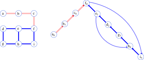
Figure 2: A graph (left panel) with one of its depth-first search trees (right panel). Red (hollow) and blue (solid) edges correspond to bridges and non-bridges, respectively. The dashed edges in the right panel are back-edges. Note that the depth-first search tree together with its back-edges can be decomposed into two chains, corresponding to the two back-edges, and any non-bridge is in at least one chain.

2.6 Numerical analysis for finite lattices

In order to confirm the asymptotic results (2.15) for the square lattice and to study the finite-size corrections for finite lattices, we performed Monte Carlo simulations of the RC model on the $L\times L$ square lattice with periodic boundary conditions, in the range of continuous phase transitions $0<q\leq 4$. We used a recent implementation [23] of (the Metropolis variant of) Sweeny’s algorithm [24] for $q<1$ and the Chayes-Machta-Swendsen-Wang algorithm [22] for $q\geq 1$. We determined the number of bridges in a given configuration by means of the algorithm introduced in Ref. [39]. In contrast to the approach used in [18, 40], this is a linear time algorithm applicable to any finite graph. It does not depend on a medial graph analysis, which facilitates the study of higher dimensional and non-planar systems. Here we briefly describe the algorithm and refer the reader to Ref. [39] for more details. The main idea is to construct a depth-first search (DFS) tree for any component in the spanning subgraph $(V,A)$. Any edge in $A$ that is not in a DFS tree is called a back-edge (there are precisely $|A|-|V|+K(A)$ back-edges). Because a back-edge connects vertices already connected in a DFS tree, it follows that any back-edge is a non-bridge in $(V,A)$; see Fig. 2 for an illustration of this situation. In order to be able to determine whether a given edge in a DFS tree is a bridge in $(V,A)$, the algorithm introduces a chain decomposition of the graph, where for any back-edge there is exactly one chain (ignoring chains consisting only of one vertex). Now, if a given tree edge is part of such a chain, then it is in at least one cycle and hence a non-bridge. Finally, a careful construction that avoids the iteration over overlapping chains ensures that the algorithm classifies all edges into bridges and non-bridges in linear time.

Figure 3: Critical bridge- and non-bridge density for a $L=32$ system shown as square symbols. The circles show the asymptotic values derived from a finite-size scaling analysis using the ansatz (2.20). For comparison the solid (blue) and dotted (red) line show the exact asymptotic values of non-bridges and bridges, respectively, according to (2.15).

2.7 Finite-size corrections

The bridge-edge relation (2.12) also allows us to understand the finite-size corrections to the bridge density. It relates $\mathbb{E}_{p,q,G}[\mathcal{B}]$ to the density of edges which, in turn, is related to the internal energy via (2.4). Finite-size corrections to the energy density $u_{\beta,q,G}$ close to a point of a second order phase transition, on the other hand, are widely studied and well understood from the theory of finite-size scaling. To formulate it, we need to associate a linear size $L$ to $G$, such that $|V|=L^{d}$, as is the case for a lattice graph with spatial dimension $d$. Then, the standard ansatz for the singular part $f_{s}$ of the free-energy density $f=-\log{[Z_{P}(\beta,q,G)]}/(\beta L^{d})$ as a function of the reduced temperature $t=(T-T_{c})/T_{c}$, the external field $h$, and the leading irrelevant field $v$ is given by [41]

$$f_{s}(t,h,L)=L^{-d}F{\left(tL^{1/\nu},hL^{d-\beta/\nu},vL^{-\theta/\nu}\right)}.$$ (2.19)

The internal energy $u_{\beta_{c},q,\mathbb{Z}^{d}_{L}}$ can be expressed in terms of the first derivative of $f$ with respect to $t$, evaluated at $t=h=0$. Furthermore it is plausible to assume [41, 42] that the non-singular part of $f$ has no size-dependence and directly yields the value obtained in the infinite-volume limit. We hence expect the following scaling of the bridge density:

$$\mathbb{E}_{q,L}[\mathcal{B}]=\mathbb{E}_{q,\infty}[\mathcal{B}]+L^{\frac{1}{\nu}-d}\big{(}b+\cdots\big{)}.$$ (2.20)

Here, we introduced the $L$-subscript to denote the expectation for the model on any lattice graph with linear dimension $L$, corresponding to the universality class of the $q$-state Potts model on $\mathbb{Z}^{d}_{L}$. For the case of $\mathbb{Z}^{2}_{L}$, the asymptotic density $\mathbb{E}_{q,\infty}[\mathcal{B}]$ is the one of $\mathbb{Z}^{2}$, as given by Eq. (2.15). For other 2D lattices such as the triangular and honeycomb lattice $\mathbb{E}_{q,\infty}[\mathcal{B}]$ can be derived in a similar way using well-known expressions for the critical internal energy there, see, e.g., Ref. [12]. The scaling form (2.20) itself, however, is universally valid.

We now turn to a more detailed analysis of the corrections for the case of the square lattice. We used the above bridge detection algorithm to numerically determine the size dependence of the bridge density for the critical RC model on $\mathbb{Z}^{2}_{L}$ for a number of values of the cluster weight $q$. Testing for scaling of the form (2.20), we fitted the ansatz $a+bL^{c}$ to our Monte-Carlo estimates, using the method of least squares. Up to cluster weights of about $q\approx 3.25$, all results were found to be in agreement with the implication of Eqs. (2.20) and (2.15) that $a=1/[2(1+\sqrt{q})]$ and $c=1/\nu-d$, where $d=2$. Fixing the parameter $a$ at this exact value, yields more precise fit results for the exponent $c$. These data are shown in Fig. 4, together with the exact values of $1/\nu-d$ known from the Coulomb gas mapping [4, 16]. The deviations observed for $q\gtrsim 3.25$ are attributed to the presence of higher-order corrections to the form (2.20) which increase in strength on approaching the tricritical point $q_{c}=4$.

Regarding the prefactor $b$ of the leading term $L^{1/\nu-d}$ extracted from the fits, we find that it is negative for the bridge density, hence the asymptotic result $1/[2(1+\sqrt{q})]$ is approached from below. The corresponding constant for $\mathbb{E}_{q,\mathbb{Z}^{2}_{L}}[\mathcal{C}]$ is positive such that the limit is approached from above. This holds for all values analyzed in $q\in[0,4]$. Thus in illustrative words, the configurations on $\mathbb{Z}^{2}_{L}$ still “feel” the “extra” edges closing the lattice to form a torus and hence they are typically less “fragile” than corresponding configurations on $\mathbb{Z}^{2}$. Interestingly, when one considers the finite-size dependence of $\mathbb{E}_{q,\mathbb{Z}^{2}_{L}}[\mathcal{N}]$ one finds an excess of edges (relative to the asymptotic result for $\mathbb{Z}^{2}$) for $q>1$ and a shortfall for $q<1$. Now, due to the fact that $\mathbb{E}_{p,q,G}[\mathcal{N}]=\mathbb{E}_{p,q,G}[\mathcal{B}]+\mathbb{E}_{p,q,G}[\mathcal{C}]$, we have that in particular the amplitudes of the finite-size corrections of $\mathbb{E}_{q,\mathbb{Z}^{2}_{L}}[\mathcal{B}]$ and $\mathbb{E}_{q,\mathbb{Z}^{2}_{L}}[\mathcal{C}]$ cancel each other for $q=1$, whereas the modulus of the amplitude for $\mathbb{E}_{q,\mathbb{Z}^{2}_{L}}[\mathcal{B}]$ is larger (smaller) than the one for $\mathbb{E}_{q,\mathbb{Z}^{2}_{L}}[\mathcal{C}]$ for $q<1$ ($q>1$), respectively. We omit the details on the size dependence of $\mathbb{E}_{q,\mathbb{Z}^{2}_{L}}[\mathcal{C}]$, as no new mechanism appears and the above results on $\mathbb{E}_{q,\mathbb{Z}^{2}_{L}}[\mathcal{B}]$ can be easily adapted to this case.

Figure 4: Comparison of numerically extracted exponents of the leading finite-size correction for the density of bridges and pseudo-bridges. The solid and dotted line show the exact Coulomb-gas value for pseudo-bridges and bridges, respectively. The deviations for values of $q$ around $4$ are caused by strong sub-leading finite-size corrections.

Following Xu et al. [18], we extend our study of finite-size corrections on the torus $\mathbb{Z}^{2}_{L}$ from bridges to the larger class of “type-1 edges”, that is edges that that have both of their associated loop arcs in the same loop in the associated loop configuration. While on a planar lattice all such bonds are bridges, this is not the case for $\mathbb{Z}^{2}_{L}$, where also non-bridges can be of type 1. Such edges are hence called pseudo-bridges [18, 40]. If we denote by $L_{1}(A)$ and $L_{2}(A)$ the set of (open) edges in $(V,A)$ that have both of their associated loop arcs in the same loop (type-1 edges) or in two different loops (type-2 edges), respectively, we have that

$$\mathbb{P}_{p,q,\mathbb{Z}^{2}_{L}}[e\in L_{1}]=\mathbb{P}_{p,q,\mathbb{Z}^{2}_{L}}[e\in L_{1},e\in B]+\mathbb{P}_{p,q,\mathbb{Z}^{2}_{L}}[e\in L_{1},e\in C]=\mathbb{P}_{p,q,\mathbb{Z}^{2}_{L}}[e\in B]+\mathbb{P}_{p,q,\mathbb{Z}^{2}_{L}}[e\in L_{1},e\in C].$$ (2.21)

The second equality follows from $B\subseteq L_{1}$, that is any bridge has necessarily both loop arcs in the same loop (as it cannot enclose any face). Equivalently, we have $\mathbb{E}_{p,q,\mathbb{Z}^{2}_{L}}[\ell_{1}]=\mathbb{E}_{p,q,\mathbb{Z}^{2}_{L}}[\mathcal{B}]+\mathbb{E}_{p,q,\mathbb{Z}^{2}_{L}}[\mathcal{P}]$, where $\mathcal{P}(A)\equiv\left|e\in E:e\in L_{1}(A),e\in C(A)\right|/m$, i.e., the density of pseudo-bridges in $A$, and $\ell_{1}$ denotes the fraction of edges that are of type 1. In order to understand the general size dependence of $\mathbb{E}_{q,\mathbb{Z}^{2}_{L}}[\ell_{1}]$, we determined the number of type-1 edges in our numerical simulations and fitted a finite scaling ansatz $\mathbb{E}_{q,\mathbb{Z}^{2}_{L}}[\ell_{1}]=a+bL^{-\epsilon_{1}}+cL^{-\epsilon_{2}}$ to our Monte-Carlo data. The resulting estimates are consistent with $a=1/[2(1+\sqrt{q})]$ and $\epsilon_{1}=2-1/\nu$ as well as $\epsilon_{2}=x_{2}$. In a second step, we also performed fits with $c$ fixed to its exact value and $\epsilon_{1}$ and $\epsilon_{2}$ fixed to the values implied by the Coulomb gas for the identifications $\epsilon_{1}=2-1/\nu$ and $\epsilon_{2}=x_{2}$, such that $b$ and $c$ were the only free parameters in a now linear fit. As it is apparent from the parameters collected in Table 1, the quality of these fits is very good, even including the smallest system sizes $L=4$, $8$, $16$, $32$, strongly suggesting the following asymptotic form for the square lattice

$$\mathbb{E}_{q,\mathbb{Z}^{2}_{L}}[\ell_{1}]\sim\mathbb{E}_{q,\mathbb{Z}^{2}}[\mathcal{B}]+bL^{1/\nu-d}+cL^{-x_{2}},$$ (2.22)

where again $\mathbb{E}_{q,\mathbb{Z}^{2}}[\mathcal{B}]=1/[2(1+\sqrt{q})]$. Figure 5 shows our numerical data for the two cluster weights $0.5$ and $2$, together with the corresponding best fits.

$q$	$b$	$c$	$\chi^{2}/N_{\rm d.o.f.}$	$L_{\rm min}$	$Q$
$3.5$	$-0.1410(7)$	$0.504(7)$	$1.0354$	$4$	$0.4135$
$3.5$	$-0.1405(8)$	$0.49(2)$	$0.9722$	$8$	$0.4730$
$3.5$	$-0.1406(9)$	$0.50(4)$	$1.0155$	$16$	$0.4270$
$3.5$	$-0.140(1)$	$0.4(1)$	$1.1116$	$32$	$0.3514$
$2$	$-0.218(3)$	$0.393(7)$	$0.5554$	$4$	$0.9007$
$2$	$-0.219(3)$	$0.40(1)$	$0.6303$	$8$	$0.8183$
$2$	$-0.219(4)$	$0.40(2)$	$0.7086$	$16$	$0.7173$
$2$	$-0.218(6)$	$0.38(4)$	$0.8504$	$32$	$0.5580$
$1.25$	$-0.27(1)$	$0.32(2)$	$0.8451$	$4$	$0.6199$
$1.25$	$-0.26(2)$	$0.31(3)$	$0.9229$	$8$	$0.9229$
$1.25$	$-0.25(3)$	$0.30(4)$	$0.8482$	$16$	$0.5819$
$1.25$	$-0.31(4)$	$0.41(7)$	$0.4951$	$32$	$0.8607$
$0.9$	$-0.21(3)$	$0.19(3)$	$0.4983$	$4$	$0.9356$
$0.9$	$-0.22(5)$	$0.20(4)$	$0.5010$	$8$	$0.9155$
$0.9$	$-0.23(7)$	$0.21(6)$	$0.5237$	$16$	$0.8748$
$0.9$	$-0.3(1)$	$0.2(9)$	$0.6113$	$32$	$0.7692$
$0.5$	$-0.336(8)$	$0.192(4)$	$1.0286$	$4$	$0.4203$
$0.5$	$-0.32(1)$	$0.188(5)$	$1.0466$	$8$	$0.4019$
$0.5$	$-0.32(2)$	$0.188(7)$	$1.2546$	$16$	$0.2502$
$0.5$	$-0.33(4)$	$0.190(9)$	$1.5533$	$32$	$0.1332$
$0.05$	$-0.429(6)$	$0.033(1)$	$0.7662$	$4$	$0.7073$
$0.05$	$-0.41(1)$	$0.033(1)$	$0.6955$	$8$	$0.7575$
$0.05$	$-0.43(3)$	$0.033(1)$	$0.6882$	$16$	$0.7365$
$0.05$	$-0.43(7)$	$0.033(1)$	$0.8571$	$32$	$0.5522$
$0.005$	$-0.466(5)$	$0.0040(4)$	$0.9548$	$4$	$0.4979$
$0.005$	$-0.49(1)$	$0.0045(5)$	$0.6865$	$8$	$0.7663$
$0.005$	$-0.49(3)$	$0.0046(6)$	$0.6857$	$16$	$0.7389$
$0.005$	$-0.38(8)$	$0.0041(7)$	$0.5806$	$32$	$0.7948$

Table 1: Estimates of the fitting parameters $b$ and $c$ in the finite-size scaling ansatz (2.22) of the density of type-1 edges. $Q$ denotes the quality of fit [43] or confidence level, that is the probability that $\chi^{2}$ would exceed the empirical value, under the assumption that the imposed statistical model is correct. In what follows we refer to fits with confidence level $\geq 10\%$ simply as “good” fits.

It is interesting to compare the general form (2.22) to the results found in Ref. [18] for the percolation case, corresponding to $q\to 1$. There, finite-size corrections to the bridge density on the torus $\mathbb{Z}^{2}_{L}$ were found to decay with exponent $-x_{2}=-5/4$. While this is numerically consistent with our findings since $1/\nu-d=-x_{2}$ for percolation [44, 45, 17, 46], it is clear from the present analysis that the relevant exponent describing finite-size corrections to the bridge density is $1/\nu-d$. Indeed, the values of $-x_{2}$ and $1/\nu-d$ strongly differ for $q\neq 1$, cf. Fig. 4. Moreover, for the square lattice with periodic boundary conditions Xu et al. [18] showed rigorously that $\mathbb{P}_{1/2,1,\mathbb{Z}^{2}_{L}}[e\in L_{1}]=\mathbb{E}_{1/2,1,\mathbb{Z}^{2}_{L}}[\ell_{1}]=1/4$, independent of $L$. This is consistent with our general form (2.22) for the percolation case with $1/\nu-d=-x_{2}$ if the amplitudes $b$ and $c$ cancel. Indeed, this is what we find from the fit data in Table 1, which clearly support the statement that $b=-c$ as $q\to 1$, as required by the rigorous finding that $\mathbb{E}_{1/2,1,\mathbb{Z}^{2}_{L}}[\ell_{1}]=1/4$. Hence, it is a particular cancellation of finite-size effects that leads to the size-independence observed for percolation. Further, it is known that for $q\rightarrow 0$ with $p=p_{\rm sd}(q)$, one recovers the uniform spanning tree model, for which clearly no pseudo-bridges exist, that is one can easily verify that, on $\mathbb{Z}^{2}_{L}$, $\mathbb{E}_{q,\mathbb{Z}^{2}_{L}}[\ell_{1}]\rightarrow\frac{1}{2}-\frac{1}{2}L^{-2}$ for $q\rightarrow 0$, which is in agreement with (2.22), due to $1/\nu\rightarrow 0$ and the numerical observation (see Table 1) that $a\rightarrow-1/2$ and $b\rightarrow 0$ for $q\rightarrow 0$. We remark that the fitting estimates for $q$ close to one need to be treated with caution, as here the two exponents $1/\nu-2$ and $-x_{2}$ come very close to each other, and hence it is numerically very difficult to distinguish the two contributions and the corresponding constants $a$, $b$. However, outside a suitable “safety”-window around $q=1$, it appears that both $a$, $b$ are increasing with $q$.

Figure 5: Estimated size dependent deviation $\mathbb{E}_{q,\mathbb{Z}^{2}_{L}}[\ell_{1}]-1/[2(\sqrt{q}+1)]$ for $q=0.5$ and $q=2$ for the self-dual RC model on $\mathbb{Z}^{2}_{L}$, together with the best fit to the scaling form corresponding to (2.22). All available system sizes starting from $L=4$ were included in the two fits and yielded $\chi^{2}/N_{\rm d.o.f.}=1.0286$ and $0.5554$, for $q=0.5$ and $2$ respectively, where $N_{\rm d.o.f.}=14$, is the number of degrees of freedom for both cluster weights considered.

We close the analysis of size-dependent effects by establishing a relationship for percolation between pseudo-bridges and a particular arm event which shows the observed $L^{-x_{2}}$ decay. A pseudo-bridge is a non-bridge that resides on a cross cluster that winds simultaneously along both directions on the torus [18]. Furthermore, any pseudo-bridge has both associated loop-arcs in the medial graph in the same loop. In other words, a pseudo-bridge is a non-bridge on a cross cluster that is pivotal to the existence of the cross cluster, i.e., if $A$ is a configuration that contains a cross cluster, then removing a pseudo-bridge $e$ implies that $A_{e}$ has no remaining cross cluster. Therefore pseudo-bridges are in a certain sense the “bridges” of the cross cluster. We can translate this into a (polychromatic) four-arm event [47, 3] as follows: Any edge, say $e$, that is pivotal to the cross cluster has the property that starting from $e$ two paths of open edges extend to a distance $L/2$ (here we use the toroidal geometry and in particular the absence of boundaries). Since $e$ is pivotal for the cross configuration, there must also be two paths of closed (dual) edges starting at the dual vertices associated to $e$ and extending to a distance $L/2$, which precisely ensure that there can be no alternative, $e$-avoiding, path that would preserve the cross configuration property upon removal of $e$. Thus what we constructed is a particular instance of an poly-chromatic four-arm event, of alternating primal and dual “color”, in the annulus centered around the edge $e$ with outer radius $L/2$. The probability of such an event decays for large $L$ as $L^{-x_{4}^{\rm{(P)}}}$, where $x_{4}^{\rm{(P)}}$ is the poly-chromatic four-arm exponent, which equals $5/4$ for critical percolation. Using the fact that $x_{4}^{\rm{(P)}}=x_{2}$, where the latter is the two-arm exponent as defined for instance in [46] and referred to by Xu et al. in [18] we have the appearance of the exponent $x_{2}$.

We note that the notion of pseudo-bridges and the corresponding scaling analysis given above is specific to the case of locally planar lattices. The concentration on the square lattice was for practical reasons only, however, and we expect the same results, only with different amplitudes, for the cases of other lattices such as the triangular or honeycomb cases with periodic boundary conditions.

3 Other types of pivotal edges

So far our analysis has focused on open edges, that is bridges and non-bridges. Surprisingly, the analysis of closed edges turns out to be very interesting too, in that it allows us to link several seemingly unrelated quantities, studied in the literature in different contexts, to the density of bridges. Moreover the study of closed edges provides a further probe for the cluster structure, for instance a large density of candidate non-bridges suggests that the clusters are more likely to self-entangle than to overlap with other clusters. In order to analyze the corresponding densities consider a given closed edge $e=(x,y)$. Clearly we have that when $x\nleftrightarrow y$ then $e$ is a candidate bridge (and vice versa), i.e., a candidate bridge corresponds to a pair of nearest-neighbor vertices that are not connected. This observation allows us to state the following almost trivial but useful identity that holds for arbitrary $e=(x,y)\in E$:

$$\mathbb{P}_{p,q,G}[e\in\overline{B}]=\mathbb{P}_{p,q,G}[x\nleftrightarrow y].$$

In fact, it is possible to relate the r.h.s. above to $\mathbb{P}_{p,q,G}[e\in B]$, the probability that $e$ is a bridge. To see this, note that for fixed $e=(x,y)$ any configuration $A\subseteq E$ that has the property $x\nleftrightarrow y$ can be related one-to-one to the configuration $A+e$, in which $e$ is a bridge. Furthermore, as the insertion of $e$ reduces the number of components by one, it follows that $\mathbb{P}_{p,q,G}[A]=q(1-p)\mathbb{P}_{p,q,G}[A^{e}]/p$ which in turn implies

$$\mathbb{P}_{p,q,G}[x\nleftrightarrow y]=\sum_{A\subseteq E}\mathbb{P}_{p,q,G}[A]\mathds{1}_{\left\{x\stackrel{{\scriptstyle A}}{{\nleftrightarrow}}y\right\}}=\frac{q(1-p)}{p}\sum_{A\subseteq E}\mathbb{P}_{p,q,G}[A+e]\mathds{1}_{\left\{e\in B(A+e)\right\}}=\frac{q(1-p)}{p}\mathbb{P}_{p,q,G}[e\in B].$$ (3.1)

Hence we have $\mathbb{P}_{p,q,G}[e\in\overline{B}]=\frac{q(1-p)}{p}\mathbb{P}_{p,q,G}[e\in B]$, and therefore using the bridge formula (2.12) and the definition (2.6) of the nearest-neighbor connectivity ${\cal E}$ we obtain the general result

$$\mathbb{E}_{p,q,G}[\overline{\mathcal{B}}]=1-\mathbb{E}_{p,q,G}[\mathcal{E}]=\frac{q}{1-q}\left(\frac{\mathbb{E}_{p,q,G}[\mathcal{N}]}{p}-1\right).$$ (3.2)

The corresponding asymptotic values for the square lattice follow immediately:

$$\mathbb{E}_{q,\mathbb{Z}^{2}}[\overline{\mathcal{B}}]=\frac{\sqrt{q}}{2(1+\frac{1}{\sqrt{q}})},\quad\mathbb{E}_{q,\mathbb{Z}^{2}}[\overline{\mathcal{C}}]=\frac{1}{2(1+\sqrt{q})}.$$ (3.3)

As a result of the relation to the edge density, we again conclude that the leading finite-size corrections are given by $L^{1/\nu-d}$. These findings are in line with those of Hu et al. in Ref. [27], who find for percolation that for $L\rightarrow\infty$ on $\mathbb{Z}^{2}_{L}$ one has $\mathbb{E}_{p,\mathbb{Z}^{2}_{L}}[\mathcal{E}]\rightarrow 3/4$. On the other hand, it was shown in Ref. [18] that the asymptotic bridge density for critical percolation on $\mathbb{Z}^{2}_{L}$ is $1/4$ (which also follows from our result (2.12)). These two results are hence clearly consistent with the relation (3.1). Finally from (3.2) and (3.3) one concludes that

$$\mathbb{E}_{q,\mathbb{Z}^{2}_{L}}[\mathcal{E}]\rightarrow\frac{2+\sqrt{q}}{2\left(1+\sqrt{q}\right)}\textnormal{ for }L\rightarrow\infty,$$

which is consistent with the results of Ref. [27].

4 Maximal bridge density for percolation

It is apparent from Fig. 1 that the expected bridge density $\mathbb{E}_{p,q,\mathbb{Z}^{2}_{L}}[\mathcal{B}]$ is maximal for $p_{\rm f}(q)<p_{\rm sd}(q)$ for any $q\in(0,4]$ [20]. The reason for this is a priori not clear and here we focus on the percolation case $q=1$ and obtain an expression for $\frac{d}{dp}\mathbb{E}_{p,G}[\mathcal{B}]$, that is for general graphs $G$, to determine its zero(s) one of which must correspond to the location of the sought maximum. In principle we could again apply the Russo-Margulis formula directly to $|B|$ to obtain the required derivative. However, there is an alternative, more geometric, approach. In Ref. [44], Coniglio showed that the $p$-derivative of $\mathbb{P}_{p,G}[x\leftrightarrow y]$ for two vertices $x,y\in V$ (not necessarily neighbors) satisfies the following differential equation:

$$\frac{\rm d}{{\rm d}p}\mathbb{P}_{p,G}[x\leftrightarrow y]=\frac{1}{p}\mathbb{E}_{p,G}[\lambda_{x,y}],$$ (4.1)

where $\lambda_{x,y}(A)$ is the number of bridges on any self-avoiding path in $A$ connecting $x$ and $y$. We emphasize that for a given edge $(x,y)\in E$ the quantity $\lambda_{x,y}$ can be non-zero, even if $(x,y)\notin B(A)$. This is because $\lambda_{x,y}$ counts the number of bridges in the spanning subgraph $(V,A)$ that would disconnect $x$ from $y$ upon removal. As an example, consider vertices $b$ and $e$ in the left panel in Figure 2. Even with $(b,e)$ not being part of the considered spanning subgraph, we have $\lambda_{b,e}=2$, because edges (in fact bridges) $(b,c)$ and $(c,f)$ are essential for the connectivity of $b$ and $e$. Note that bridge $(a,b)$ is not essential for the connectivity of $b$ and $e$ as its removal does not disconnect $b$ and $e$. Note that relationship (4.1) also follows straightforwardly from the Russo-Margulis formalism applied to the indicator function of the event $x\leftrightarrow y$. As a result of the bijection relation (3.1) we can transform (4.1) into a differential equation for the bridge density:

$$\frac{\rm d}{{\rm d}p}\mathbb{E}_{p,G}[\mathcal{B}]=-\frac{1}{(1-p)|E|}\sum_{(x,y)\in E}\mathbb{E}_{p,G}[\lambda_{x,y}]+\frac{1}{p(1-p)}\mathbb{E}_{p,G}[\mathcal{B}].$$ (4.2)

We emphasize that now $\lambda_{x,y}$ is only evaluated for nearest-neighbor pairs, that is for $x,y\in V$ with $(x,y)\in E$. Observe

$$\sum_{(x,y)\in E}\lambda_{x,y}(A)=\sum_{(x,y)\in E}\sum_{e\in E}\mathds{1}_{\left\{x\stackrel{{\scriptstyle A}}{{\leftrightarrow}}y\right\}}\mathds{1}_{\left\{x\stackrel{{\scriptstyle A_{e}}}{{\nleftrightarrow}}y\right\}}=\sum_{e\in E}\left[\sum_{(x,y)\in E}\mathds{1}_{\left\{x\stackrel{{\scriptstyle A}}{{\leftrightarrow}}y\right\}}\mathds{1}_{\left\{x\stackrel{{\scriptstyle A_{e}}}{{\nleftrightarrow}}y\right\}}\right].$$ (4.3)

Now, for a given edge $e\in E$ define $\rho_{e}(A)$ as the sum in the square brackets in (4.3) or, equivalently, to be $0$ when $e$ is not a bridge in $A$ and otherwise the number of nearest-neighbor pairs for which the bridge $e$ lies on any (all) self-avoiding path(s) in $(V,A)$ between them. In other words $\rho_{e}(A)$ counts for how many nearest-neighbor pairs edge $e$ contributes to $\lambda_{x,y}$. We call $\rho_{e}$ the bridge load of $e$. Note that we have $\rho_{e}(A)\geq\mathds{1}_{\{e\in B(A)\}}$ and hence $\mathbb{E}_{p,q}[\rho_{e}]\geq\mathbb{P}_{p,q}[e\in B]$. For an example consider the left panel in Figure 2, here edges $(a,b),(b,c),(c,f)$ have bridge loads $2$, $3$, $3$, respectively. It is evident that in a certain sense $\rho_{e}$ generalizes the bridge density and encodes how relevant a given bridge is for the connectivity at large. We emphasize that one only has to count connected neighbor pairs. We finally obtain:

$$\frac{\rm d}{{\rm d}p}\mathbb{E}_{p,G}[\mathcal{B}]=-\frac{1}{(1-p)}\mathbb{E}_{p,G}[\bar{\rho}]+\frac{1}{p(1-p)}\mathbb{E}_{p,G}[\mathcal{B}],$$ (4.4)

where we defined $\bar{\rho}(A)\equiv\frac{1}{|E|}\sum_{e\in E}\rho_{e}(A)$. Therefore we find that the l.h.s. in (4.4) vanishes for $p=p_{\rm f}$, where $p_{\rm f}$ is the solution of the following equation

$$\mathbb{E}_{p_{\rm f},G}[\mathcal{B}]=p_{\rm f}\mathbb{E}_{p_{\rm f},G}[\bar{\rho}].$$ (4.5)

We remark that $p_{\rm f}$ is a graph dependent quantity and we suppress the explicit dependence. In Fig. 6 we illustrate this condition for a small system size and the case $G=\mathbb{Z}^{2}_{L}$. Moreover, under translational invariance (which is given, e.g., for $\mathbb{Z}^{2}_{L}$), (4.5) is equivalent to $\mathbb{P}_{p_{\rm f},G}[e\in B]=p_{\rm f}\mathbb{E}_{p_{\rm f},G}[\rho_{e}]$ for arbitrary $e\in E$. This has a nice intuitive interpretation: $\mathbb{E}_{p,G}[\rho_{e}]$ counts the typical number of nearest-neighbor pairs at the interface between two clusters that are glued together only by the presence of bridge $e$. There are two effects at work here: increasing $p$ typically increases the size of the clusters and therefore possibly also the number of nearest neighbors on the interface. Additionally, however, increasing $p$ will eventually create additional links between the two clusters, in which case $e$ ceases to be a bridge, such that this effect decreases $\mathbb{P}_{p,G}[e\in B]$. Now, the maximal fragility (maximum of $\mathbb{P}_{p,G}[e\in B]$) is attained for the bond density $p_{\rm f}$, where the expected number of closed edges between two clusters glued together by $e$ equals precisely the probability that $e$ is a bridge. Increasing $p$ further strengthens the cohesion between the clusters, and hence the probability of $e$ being a bridge starts to decrease afterwards.

Figure 6: Numerically estimated density of bridges and bridge load for percolation on $\mathbb{Z}^{2}_{L}$ for $L=16$ and $L=128$, corresponding to the smaller and larger markers, respectively. Additionally, the inset shows our estimates for $p_{f}$ for system sizes from $L=8$ up to $L=128$. The estimates for the location of the crossing “saturate” to a value $0.4056(5)$, and therefore we conclude that $p_{\rm f}=0.4056(5)$ for $\mathbb{Z}^{2}$, according to (4.5). We point out that we used a naive depth-first search traversal based algorithm for determining the bridge load, so we could not study systems with $L>128$ in practise. The lines in the figure are obtained by interpolating the data points using splines.

In what follows we restrict the analysis to the case $G=\mathbb{Z}^{2}_{L}$ in order to extract the asymptotic value of $p_{f}$ for $\mathbb{Z}^{2}$. Consider Figure 6, where we numerically confirm condition (4.5) and estimate $p_{\rm f}=0.4056(5)$ for $\mathbb{Z}^{2}$. We note that, albeit the maximum of $\mathbb{P}_{p,\mathbb{Z}^{2}}[e\in B]$ is attained for $p=p_{\rm f}$, the bridge load $\mathbb{E}_{p,\mathbb{Z}^{2}}[\rho_{e}]$ increases further and is apparently maximized for $p=p_{\rm sd}(1)=p_{c}=1/2$. This nicely reflects the intricate cluster structure at criticality. One might wonder how the bridge density can decrease but the overlap continues to increase. This can happen when in most (probable) configurations $e$ is not a bridge, but for configurations where $e$ is a bridge one has typically a very large self-entanglement of the clusters attached to the two ends of $e$, outweighing the effective decrease of $\mathbb{P}_{p,\mathbb{Z}^{2}_{L}}[e\in B]$. This effect is most drastic for $p=p_{c}$. We note that Coulomb gas arguments predict that the l.h.s. of (4.4) remains finite at $p=p_{\rm sd}(1)=1/2$, which clearly implies that $\mathbb{E}_{p,\mathbb{Z}^{2}}[\rho_{e}]$ remains finite at $p=1/2$. More precisely we can show that the peak of $\mathbb{E}_{q,\mathbb{Z}^{2}_{L}}[\rho_{e}]$ scales as $L^{2-2x_{2}}$ for $q\in[0,4]$, where in particular $x_{2}=5/4$ for percolation [see the discussion in the next section and in particular (5.3)]. Unfortunately, so far we have not been able to establish an exact value for $p_{\rm f}(1)$ let alone in the correlated setting $q\neq 1$ for $\mathbb{Z}^{2}$. This is a challenging problem we wish to address in a forthcoming study.

5 Bridge fluctuations

As we have seen, the bridge-edge formula (2.12) together with the theory of finite-size scaling, provides a rather complete understanding of the critical bridge density. Higher moments of the bridge distribution can be discussed with similar techniques as we will show now for the example of the variance. Naively, one might expect that this variance $\operatorname{Var}_{p,q,G}[|B|]$ only depends on the fluctuations of $N$. In this case the critical variance would follow $\operatorname{Var}_{q,L}[|B|]/L^{d}\approx L^{\alpha/\nu}$, which, in two dimensions, in turn would imply a divergence with $L$ for $q\geq 2$ and a “saturation” for $q<2$ [46]. As we will show however, the story is not quite as simple.

To work out the fluctuations of the bridge density, we apply the Russo-Margulis formula to the second derivative of the partition function $Z_{p,q,G}\equiv Z_{\rm RC}(p,q,G)$, which we then in turn equate to the expression one obtains by explicit differentiation. To start with, we have, using (2.11),

$$\partial_{p}^{2}Z_{p,q,G} =(1-q)\partial_{p}\left(\frac{Z_{p,q,G}}{p}\mathbb{E}_{p,q,G}[|B|]\right)$$

$$=-Z_{p,q,G}\frac{1-q}{p^{2}}\mathbb{E}_{p,q,G}\left[|B|\right]+\frac{1-q}{p}\partial_{p}\mathbb{E}_{p,G}\left[q^{K}|B|\right].$$

Let us now focus on the second term:

$$\frac{1-q}{p}\partial_{p}\mathbb{E}_{p,G}\left[q^{K}|B|\right] =\frac{1-q}{p}\sum_{e,f\in E}\mathbb{E}_{p,G}\left[\delta_{e}\left(q^{K}\mathds{1}_{\{f\in B\}}\right)\right]$$

$$=\frac{1-q}{p^{2}}\sum_{e,f\in E}\sum_{A\subseteq E:\atop e\in A}\mathbb{P}_{p,G}[A]\left[q^{K(A)}\mathds{1}_{\{f\in B(A)\}}-q^{K(A_{e})}\mathds{1}_{\{f\in B(A_{e})\}}\right].$$ (5.1)

We can split the inner sum into two sums corresponding to $e\in B(A)$ and $e\in C(A)$, of which we first consider the former

$$\frac{1-q}{p^{2}}\sum_{e,f\in E}\sum_{A\subseteq E:\atop e\in B(A)}\mathbb{P}_{p,G}[A]\left[\mathds{1}_{\{e=f\}}q^{K(A)}\mathds{1}_{\{f\in B(A)\}}+\mathds{1}_{\{e\neq f\}}q^{K(A)}(1-q)\mathds{1}_{\{f\in B(A)\}}\right].$$

A few comments are in order: If $e=f$ we clearly have that $e=f\notin B(A_{e})$ hence we recover the expected bridge density. For $e\neq f$ it is important to observe that removing a bridge $e$ cannot influence the pivotality of an occupied edge $f$, in particular when $f\in B(A)$ then also $f\in B(A_{e})$, whenever $e$ is a bridge in $A$. The above can therefore be re-written as

$$\frac{1-q}{p^{2}}Z_{p,q,G}\mathbb{E}_{p,q,G}\left[|B|\right]+\frac{(1-q)^{2}}{p^{2}}Z_{p,q,G}\sum_{e\neq f\in E}\mathbb{P}_{p,q,G}[e\in B,f\in B].$$

For the non-bridge sum of (5.1) note that only summands with $e\neq f$ contribute, because otherwise if $e\in C(A)$ then trivially $f=e\notin B(A)$, $B(A_{e})$. Furthermore, if $e\neq f$ such that $e\in C(A)$ and $f\in B(A)$ then we have also a vanishing contribution because deleting a non-bridge cannot change the fact that $f$ is a bridge. Thus, there can only be a contribution for a configuration $A$ such that $e\in C(A)$ and $f\in C(A)$ as well as both edges are in one cycle and deleting $e$ will destroy the cycle and hence cast $f$ into a bridge in $A_{e}$. Moreover, both edges $e$ and $f$ must only be in one cycle that has no edge overlap with other cycles (imagine two clusters glued together in parallel by the edges $e$ and $f$, hence in particular there are no additional links between the two clusters). Write $e\overset{A}{\Leftrightarrow}f$ for the above event involving edge $e$ and $f$. We obtain for the second term:

$$-Z_{p,q,G}\frac{1-q}{p^{2}}\sum_{e\neq f\in E}\mathbb{P}_{p,q,G}\left[e\Leftrightarrow f\right].$$

We therefore obtain eventually for $\partial_{p}^{2}Z_{p,q}$:

$$\partial_{p}^{2}Z_{p,q,G} =Z_{p,q,G}\frac{1-q}{p^{2}}\left((1-q)\sum_{e\neq f\in E}\mathbb{P}_{p,q,G}[e\in B,f\in B]-\sum_{e\neq f\in E}\mathbb{P}_{p,q,G}[e\Leftrightarrow f]\right)$$

$$=Z_{p,q,G}\frac{1-q}{p^{2}}\left((1-q)\operatorname{Var}_{p,q,G}[|B|]+(1-q)\mathbb{E}_{p,q,G}[|B|]^{2}-(1-q)\mathbb{E}_{p,q,G}[|B|]-\sum_{e\neq f\in E}\mathbb{P}_{p,q,G}[e\Leftrightarrow f]\right).$$

On the other hand one can show by explicit differentiation and after some straightforward but tedious algebra that one has:

$$\frac{1}{Z_{p,q,G}}\partial_{p}^{2}Z_{p,q,G}=\frac{\mathbb{E}_{p,q,G}[N]\left(2p-1-2p|E|\right)-|E|p^{2}+|E|^{2}p^{2}+\operatorname{Var}_{p,q,G}[N]+\mathbb{E}_{p,q,G}[N]^{2}}{p^{2}(1-p)^{2}}.$$

Equating both expressions for $\partial_{p}^{2}Z_{p,q,G}$ with subsequent rearranging yields

$$\operatorname{Var}_{p,q,G}[|B|] =\frac{\mathbb{E}_{p,q,G}[N]\left(2p-1-2p|E|\right)-|E|p^{2}+\operatorname{Var}_{p,q,G}[N]+\left(\mathbb{E}_{p,q,G}[N]-|E|p\right)^{2}+2|E|p\mathbb{E}_{p,q,G}[N]}{(1-q)^{2}(1-p)^{2}}$$

$$-\mathbb{E}_{p,q,G}[|B|]^{2}+\mathbb{E}_{p,q,G}[|B|]+\frac{1}{1-q}\sum_{e\neq f\in E}\mathbb{P}_{p,q,G}[e\Leftrightarrow f].$$

Using the bridge edge identity (2.12) we can simplify the above to

$$\frac{\operatorname{Var}_{p,q,G}[|B|]}{|E|}=\frac{\mathbb{E}_{p,q,G}[\mathcal{N}]\left(2p-1\right)-p^{2}+\operatorname{Var}_{p,q,G}[N]/|E|}{(1-q)^{2}(1-p)^{2}}+\mathbb{E}_{p,q,G}[\mathcal{B}]+\frac{1}{1-q}\frac{1}{|E|}\sum_{e\neq f\in E}\mathbb{P}_{p,q,G}[e\Leftrightarrow f].$$ (5.2)

We emphasize that (5.2) is an exact result valid for any $p$ and $q$ as well as any graph $G$, thus it has the same status as the bridge-edge identity (2.12). Furthermore, we remark that for $e=(u,v)$ and $f=(x,y)$ we have by a bijection argument, similar to the one used in Sec. 3 to derive the relationship between the bridge density and nearest-neighbor connectivity:

$$\mathbb{P}_{p,q,G}[e\Leftrightarrow f]=\frac{p^{2}}{(1-p)^{2}}\frac{1}{q}\mathbb{P}_{p,q,G}[(u,v)\veebar(x,y)].$$

Here $\mathbb{P}_{p,q,G}[(u,v)\veebar(x,y)]$ for $(u,v),(x,y)\in E$ is the probability that the two nearest-neighbor pairs belong to two different clusters, such that the two distinct clusters each contain one vertex from $\{u,v\}$ and one vertex from $\{x,y\}$ (see Fig. $1(c)$ in Ref. [48]).

We pause for a moment, and remark that completely analogous arguments can be used to obtain an expression for the $p$-derivative of $\mathbb{E}_{p,q,G}[\mathcal{B}]$, studied in Section 4, in terms of the probabilities of events $e\Leftrightarrow f$. A consequence of this is that we can obtain an explicit expression for $\mathbb{E}_{p,q,G}[\bar{\rho}]$:

$$\mathbb{E}_{p,q,G}[\bar{\rho}]=\mathbb{E}_{p,q,G}[\mathcal{B}]+\frac{1}{|E|}\frac{1-p}{p}\sum_{e\neq f\in E}\mathbb{P}_{p,q,G}[e\Leftrightarrow f].$$ (5.3)

In particular, this shows explicitly that the bridge load can increase further beyond the point $p_{\rm f}(G)$, for which $\mathbb{E}_{p,G}[\mathcal{B}]$ is maximal. Moreover, as we show below, we find that at criticality, in two dimensions, $\mathbb{E}_{q,\mathbb{Z}^{2}_{L}}[\bar{\rho}]\approx L^{2-2x_{2}}$, which together with $x_{2}=5/4$ for the case $q=1$ in two dimensions, shows that the peak at $p=1/2$ in Figure 6 stays bounded as $L\rightarrow\infty$.

Coming back to the study of fluctuations of $|B|$, we focus in what follows on the self-dual line for the RC model on $\mathbb{Z}^{2}_{L}$ and study the continuum limit. As shown by Vasseur et al. [48] one has for two pairs of neighboring vertices $(u,v)$ and $(x,y)$ at distance $r$ the following asymptotic for large $r$

$$\mathbb{P}_{q,\mathbb{Z}^{2}}[(u,v)\veebar(x,y)]\sim A(q)r^{-2x_{2}(q)}.$$

This follows from the construction of a four-leg watermelon event, due to the four hulls propagating from the neighborhood of $(u,v)$ to the neighborhood of $(x,y)$, which are associated to the two clusters involved. We hence expect the following asymptotic behavior

$$\frac{1}{|E|}\sum_{e\neq f\in E}\mathbb{P}_{q,\mathbb{Z}^{2}_{L}}[e\Leftrightarrow f] =\frac{1}{|E|}\sum_{(u,v)\neq(x,y)\in E}\mathbb{P}_{q,\mathbb{Z}^{2}_{L}}[(u,v)\veebar(x,y)]$$

$$\approx A(q)\int_{1}^{\frac{L}{2}}{\rm dr}2\pi rr^{-2x_{2}(q)}$$

$$=\alpha(q)L^{2-2x_{2}(q)}+\beta(q),$$ (5.4)

where $\alpha(q)$ and $\beta(q)$ are two $q$ dependent constants.

Inspecting the form (5.2), we hence see that the fluctuation of the bridge density has two contributions, one related to the variance of the edge density that scales as $L^{\alpha/\nu}$ at criticality, and another one related to the above mentioned watermelon event with scaling proportional to $L^{2-2x_{2}}$. In order to decide which contribution constitutes the dominant leading scaling, it is useful to recall some relevant exact results from the Coulomb gas approach to two dimensional critical phenomena [4]. One finds that $\alpha/\nu=4-12/g$ and $x_{2}=2-(4-g)(4+3g)/8g$, where for critical 2D RC models one has to relate the Coulomb gas coupling $g$ to the cluster weight $q$ via $q=2+2\cos{(g\pi/2)}$ [46]. A small calculation shows then that $L^{\alpha/\nu}$ constitutes the leading contribution to the system size scaling of the variance whenever $q\geq 1$. In particular, for $q>2$, where $\alpha/\nu>0$, this translates into a divergence of $\operatorname{Var}_{q,\mathbb{Z}^{2}_{L}}[|B|]/L^{2}$ with $L$, resembling the specific-heat singularity in the same cluster weight regime. On the other hand, for $q<1$ the leading term is proportional to $L^{2-2x_{2}}$. Interestingly (and somewhat unexpected), one can explicitly verify that for $q<\tilde{q}=4\cos^{2}{(\pi/\sqrt{3})}=0.2315891\cdots$ the variance of $|B|$ diverges with the exponent $2-2x_{2}>0$. This particular value $\tilde{q}$ follows from the condition $2-2x_{2}(\tilde{q})=0\Leftrightarrow x_{2}(\tilde{q})=1$, which, using the above expressions, yields a quadratic equation for $\tilde{g}=g(\tilde{q})$ (or $\tilde{q}$): $8\tilde{g}=(4-\tilde{g})(4+3\tilde{g})$, with the two solutions $\tilde{g}=\pm 4/\sqrt{3}$. Taking only the positive solution we find that $\tilde{q}=2+2\cos{(2\pi/\sqrt{3})}=4\cos{(\pi/\sqrt{3})}^{2}$. The situation is summarized in the dotted and solid lines of Fig. 7, showing the Coulomb gas values of $\alpha/\nu$ and $2-2x_{2}$, respectively. We also analyzed the variance of the bridge density numerically. The fitting functions and resulting parameters are summarized in Table 2, and the corresponding parameter estimates are indicated by the symbols in Fig. 7. Clearly, we find excellent agreement with the expectations from Eq. (5.2) discussed above. For the marginal value $\tilde{q}=0.2315891\cdots$ we expect a logarithmic divergence, and we indeed find the corresponding form to yield the best fit to our simulation data.

Figure 7: The exponents $\alpha/\nu$ and $2-2x_{2}$ appearing in the system size scaling of $\operatorname{Var}_{q}[|B|]/m$ at criticality. The solid and dotted lines show the exact value of $2-2x_{2}$ and $\alpha/\nu$, respectively, following from the Coulomb gas mapping. The symbols denote our numerical estimates from fitting to the variance of the bridge density, cf. the data collected in Table 2.

$q$	$L_{\min}$	$\chi^{2}/N_{\rm d.o.f.}$	Model	$\kappa$	$\alpha/\nu$	$2-2x_{2}$
$0.0005$	$12$	$1.01$	$a+bL^{\kappa}$	$0.462(16)$	$-1.9576$	$\mathbf{0.4752}$
$0.005$	$4$	$1.15$	$a+bL^{\kappa}$	$0.422(3)$	$-1.8679$	$\mathbf{0.4222}$
$0.05$	$16$	$0.58$	$a+bL^{\kappa}$	$0.258(5)$	$-1.6005$	$\mathbf{0.2599}$
$0.1$	$8$	$0.76$	$a+bL^{\kappa}$	$0.164(4)$	$-1.4492$	$\mathbf{0.1648}$
$0.231589$	$8$	$1.01$	$a+b\log{(L)}$	$-$	$-1.1962$	$0$
$0.5$	$12$	$1.4$	$a+bL^{\kappa}+cL^{\alpha/\nu}$	$-0.217(51)$	$-0.8778$	$\mathbf{-0.2191}$
$1$	$6$	$0.7$	$a+bL^{\kappa}\left[1+c\log{(L)}\right]$	$-0.496(21)$	$-0.5$	$-0.5$
$1.5$	$4$	$1.05$	$a+bL^{\kappa}+cL^{2-2x_{2}}$	$-0.218(15)$	$\mathbf{-0.2266}$	$-0.7205$
$2.5$	$48$	$0.94$	$a+bL^{\kappa}$	$0.202(14)$	$\mathbf{0.2036}$	$-1.1052$
$3$	$6$	$1.14$	$a+bL^{\kappa}$	$0.398(3)$	$\mathbf{0.4}$	$-1.3$

Table 2: Numerical results for the leading exponent $\kappa$ in the finite-size scaling of $\operatorname{Var}_{q,\mathbb{Z}^{2}_{L}}[|B|]$. The two rightmost columns show the exact values obtained from the Coulomb gas mapping. The exponent values in bold face indicate the asymptotically dominant behavior. For the cluster weights $q=1.5$ and $q=0.5$ we also performed a fit to the form $a+bL^{\kappa}$, which yielded slightly worse results, due to the proximity of the two (negative) exponents. In all cases the quality-of-fit $Q$ was at least 5%.

It remains to discuss the percolation case $q=1$ where the bridge-edge identity (2.12) becomes singular and the above derivation needs to be revisited. Here, we derive the singular behavior based on another bijection argument that allows us to harness recent results on logarithmic observables emerging from a careful analysis of the appropriate logarithmic conformal field theory description of critical percolation [48, 27]. Before we do so, note that in order to extract the asymptotic scaling of the variance it suffices to study the (co-)variance $\eta_{e,f}\equiv\mathbb{P}_{p,q,G}[e\in B,f\in B]-\mathbb{P}_{p,q,G}[e\in B]\mathbb{P}_{p,q,G}[f\in B]$, which relates to $\operatorname{Var}_{p,q,G}[|B|]$ via the well known identity

$$\operatorname{Var}_{p,q,G}[|B|]=\sum_{e,f\in E}\eta_{e,f}.$$

To start with, recall that we consider critical bond percolation on $\mathbb{Z}^{2}_{L}$, i.e. $q=1$ and $p=1/2$ and write $\mathbb{P}[\cdot]$ for $\mathbb{P}_{1/2,1,\mathbb{Z}^{2}_{L}}[\cdot]$. Furthermore, note that $\mathbb{Z}^{2}_{L}$ is a transitive graph, and hence none of the following events depend on the explicit edge or vertex, used in the arguments. Now, fix two edges $e=(x_{1},y_{1}),f=(x_{2},y_{2})$ that are distance $r\ll L$ apart. Consider the event $\{e\in B\land f\in B\}$. All configurations contributing to this event can be further sub-divided into two events, depending on whether $e$ and $f$ belong to the same connected component in $(V,A)$ or not. Denote the two events by $\Omega_{1}$ and $\Omega_{2}$, respectively. Choose a configuration $A$ that belongs to $\Omega_{2}$, i.e. the two edges $e$ and $f$ are bridges in $(V,A)$ and belong to two different connected components. The crucial point is that we can relate $A$ one-to-one to $A-\{e,f\}$, a configuration where $x_{1}$, $y_{1}$, $x_{2}$, $y_{2}$ belong to four different clusters. Denote all configurations in which the four vertices belong to four different components by $\tilde{\Omega}_{2}$ (this is a event). Due to the choice of $q=1$ and $p=1/2$ we have that $\mathbb{P}{\left[{\Omega_{2}}\right]}=\mathbb{P}{\left[{\tilde{\Omega}_{2}}\right]}$. Let us now consider the event $\Omega_{1}$, i.e. the set of configurations for which $e$ and $f$ belong to the same component and both $e$ and $f$ are bridges. Now, because both edges are pivotal we can relate any such configuration $A\in\Omega_{1}$ one-to-one to a configuration where $x_{1}$ and $y_{1}$ as well as $x_{2}$ and $y_{2}$ are disconnected, and for which $x_{1},y_{1},x_{2},y_{2}$ belong to three different clusters, of which one cluster contains one vertex of $\{x_{1},y_{1}\}$ and one of $\{x_{2},y_{2}\}$. Denote the corresponding event $\tilde{\Omega}_{1}$. Note that any configuration $A\in\Omega_{1}$, where $e$ and $f$ are bridges belonging to the same cluster, must yield $3$ disconnected clusters in $A^{\prime}=A-\{e,f\}$. This is because the alternative case of $2$ disconnected clusters in $A^{\prime}$ would imply that $e$ and $f$ are in a cycle in $A$, which is obviously a contradiction. As before we have $\mathbb{P}{\left[{\Omega_{1}}\right]}=\mathbb{P}{\left[{\tilde{\Omega}_{1}}\right]}$. Finally, the probabilities $\mathbb{P}{\left[{\tilde{\Omega}_{1}}\right]}$ and $\mathbb{P}{\left[{\tilde{\Omega}_{2}}\right]}$ were studied in [48] in the framework of a corresponding logarithmic conformal field theory. We note that in the continuum limit both probabilities $\mathbb{P}{\left[{\Omega_{1}}\right]}$ and $\mathbb{P}{\left[{\Omega_{2}}\right]}$ only depend, to leading order, on $r$. Since we have $\mathbb{P}{\left[{e\in B,f\in B}\right]}=\mathbb{P}{\left[{\Omega_{1}}\right]}+\mathbb{P}{\left[{\Omega_{2}}\right]}$ we obtain by falling back to [48]:

$$\eta_{e,f}\sim\left[a+b\log{(r)}\right]r^{-2x_{2}}\Rightarrow\frac{\operatorname{Var}_{1/2,1,\mathbb{Z}^{2}_{L}}[|B|]}{L^{2}}\sim a^{\prime}+\left[b^{\prime}+c^{\prime}\log{(L)}\right]L^{2-2x_{2}},$$ (5.5)

where $x_{2}=5/4$ is the two-arm exponent for critical percolation and $a$, $b$, $a^{\prime}$, $b^{\prime}$ and $c^{\prime}$ are constants. Our numerical analysis confirmed this scaling, as shown in Table 2 and Figure 7. Thus considering the variance of bridges for critical percolation yields yet another manifestation of the underlying logarithmic conformal field theory [48]. We remark that the same logarithmic multiplicative corrections are expected in higher dimensions [49]. More precisely, one expects even the same scaling form, that is

$$\frac{\operatorname{Var}_{p_{c},1,\mathbb{Z}^{d}_{L}}[|B|]}{L^{d}}\sim a^{\prime\prime}+[b^{\prime\prime}+c^{\prime\prime}\log{(L)}]L^{2/\nu-d},$$

where we used the well known fact that $x_{2}=d-1/\nu$ holds for critical percolation [44]. It would be interesting to to verify this theoretical prediction numerically.

Before we proceed to the next section we briefly discuss the finite-size scaling of $\operatorname{Var}_{q,\mathbb{Z}^{2}_{L}}[|C|]/|E|$. This can be worked out by observing that $|C|=|A|-|B|$ which in turn implies the general identity

$$\operatorname{Var}_{p,q,G}[|C|]=\operatorname{Var}_{p,q,G}[|A|]+\operatorname{Var}_{p,q,G}[|B|]-2\operatorname{Cov}_{p,q,G}[|A|,|B|].$$

Additionally, one can verify that (see [11] or by explicit differentiation of $Z_{p,q}$)

$$\operatorname{Cov}_{p,q,G}[|A|,|B|]=p(1-p)\partial_{p}\mathbb{E}_{p,q,G}[|B|].$$

An immediate consequence of these observations is that $\operatorname{Var}_{q,\mathbb{Z}^{d}_{L}}[|C|]$ is governed by the same finite-size scaling as $\operatorname{Var}_{q,\mathbb{Z}^{d}_{L}}[|B|]$ and we therefore omit further details.

6 Bridge-free clusters

In concluding the present study, we return to the discussion of the structure of the incipient percolating cluster outlined above in the introduction. In the ‘links–nodes–blobs’ picture of Ref. [15] the attention is focused on the backbone of the cluster as the skeleton ensuring long-range connectivity. Bridges on the backbone are singled out as the bonds carrying full current for the case of an external potential difference being applied, hence their name ’red bonds’. Due to the importance of these structures for a number of applications of percolation theory, significant effort has been invested in the determination of the associated fractal dimensions $d_{\mathrm{BB}}$ and $d_{\mathrm{RB}}$ of the backbone and the red bonds, respectively [50]. Even in two dimensions, where most critical exponents and fractal dimensions, including $d_{\mathrm{F}}$ and $d_{\mathrm{RB}}$, are known exactly from Coulomb gas and further arguments [4], there is no exact expression for the fractal dimension of the backbone.

Clearly, the notions of backbone and red bonds appear to depend on the concept of long-range conductivity, and it is not obvious how they could be defined in terms of the more local connectivity structure of bridges and non-bridges. The concepts of junctions and bridges introduced in Ref. [18] are related, but not commensurate to the idea of separating bridges in the backbone (red bonds) and bridges in the blobs. We expect that, away from $q\to 0$, most bridges in the backbone are junctions as the ‘links–nodes–blobs’ picture tells us that the backbone has cycles. Still, there are junctions in the dangling ends and there are branches in the backbone. Also, as Xu et al. established for percolation in Ref. [18], branches and junctions are asymptotically finite fractions of the bridge set and hence of the edge set. It is therefore interesting to study the fractal dimensions of the related edge classes. Removal of branches from critical configurations will typically only shave off the last part of dangling ends, and we do not expect this to alter the fractal dimension of the incipient percolating cluster. This is indeed what Xu et al. report [18] and we find the same to be true also for the RC model. On the other hand, removing the junctions means deleting most of the red bonds and hence breaks down the percolating cluster into individual blobs. Their size scales with the backbone fractal dimension as $\propto L^{d_{\mathrm{BB}}}$. The same holds true for the case of bridge-free clusters where both, branches and junctions, have been removed. Studying these sets hence provides an alternative route to the determination of $d_{\mathrm{BB}}$.

Figure 8: Effective backbone scaling exponents according to Eq. (6.1) for the $q=1$ RC model extracted from the scaling of the backbone sites, the backbone bonds (data from Ref. [50]), the junction-free clusters and the bridge-free clusters (our data), respectively.

To investigate the utility of this approach for the determination of $d_{\mathrm{BB}}$, we determined the scaling of the junction-free and bridge-free clusters for the percolation case $q=1$. If we consider the effective, system-size dependent fractal dimensions [50]

$$d_{BB,\mathrm{eff}}\equiv\frac{\log[N(2L)/N(L/2)]}{\log 4},$$ (6.1)

where $N(L)$ denotes the number of sites in the junction-free or bridge-free clusters at size $L$, respectively, we can easily compare corrections to scaling for the different approaches. This is illustrated in Fig. 8, comparing the exponents extracted from the scaling of the junction-free and bridge-free clusters to the effective exponents found from the scaling of the backbone itself [50]. Clearly, the scaling of bridge-free clusters is significantly less affected by scaling corrections than the scaling of the backbone itself. Compared to this, junction-free clusters show slightly increased corrections, however interestingly with a correction amplitude of the opposite sign. We remark that our estimate for percolation $d_{\mathrm{BB}}=1.643(1)$ is consistent with existing literature values, such as $d_{\mathrm{BB}}=1.64336(1)$, $1.6434(2)$, $1.6432(8)$ in [18, 17, 50], respectively. As this is a small-scale study not using the particularly efficient algorithms available for the uncorrelated percolation case, the reduced scaling corrections do not immediately lead to an improved estimate. Instead, we focus on the estimation of $d_{\mathrm{BB}}$ for a wide range of $q$ values for which no estimates have been previously reported [17]. Whereas for the determination of $d_{\mathrm{BB}}$ directly from the backbone corrections to scaling need to be carefully taken into account, it turns out that the bridge-free clusters provide a scaling route less encumbered with such problems. As is evident from the results collected in Table 3, over the full range of $q$ values we achieve excellent fits without the inclusion of scaling corrections.

Table 3: Fit results for backbone fractal dimension $d_{BB}$.

$q$	$d_{\mathrm{BB}}$	$L_{\rm min}$	$N_{\rm d.o.f.}$	$\chi^{2}/N_{\rm d.o.f.}$	$Q$
$0.0005$	$1.264(2)$	$32$	$8$	$1.0631$	$0.3858$
$0.0050$	$1.301(1)$	$16$	$10$	$0.2934$	$0.9829$
$0.0500$	$1.383(1)$	$16$	$10$	$0.4661$	$0.9126$
$0.1000$	$1.425(1)$	$12$	$11$	$1.1773$	$0.2966$
$0.2000$	$1.480(1)$	$12$	$11$	$1.0047$	$0.4390$
$0.3000$	$1.516(1)$	$32$	$8$	$0.7543$	$0.6434$
$0.5000$	$1.567(1)$	$24$	$9$	$0.9153$	$0.5104$
$0.7000$	$1.603(1)$	$32$	$8$	$0.6676$	$0.7206$
$0.9000$	$1.630(1)$	$24$	$9$	$1.0700$	$0.3813$
$1.0000$	$1.643(1)$	$24$	$9$	$1.3227$	$0.2187$
$1.2500$	$1.670(1)$	$24$	$9$	$1.0177$	$0.4227$
$1.5000$	$1.692(1)$	$24$	$9$	$1.1271$	$0.3389$
$1.7500$	$1.716(2)$	$128$	$4$	$0.7496$	$0.5581$
$2.0000$	$1.732(1)$	$96$	$5$	$1.2095$	$0.3016$
$2.2500$	$1.744(1)$	$48$	$7$	$1.0578$	$0.3880$
$2.5000$	$1.756(1)$	$96$	$5$	$0.5469$	$0.7408$
$2.7500$	$1.774(1)$	$96$	$5$	$1.1302$	$0.3417$
$3.0000$	$1.785(1)$	$64$	$6$	$0.6563$	$0.6851$
$3.2500$	$1.797(1)$	$96$	$5$	$0.9530$	$0.4452$
$3.5000$	$1.806(1)$	$96$	$5$	$0.8288$	$0.5289$
$3.7500$	$1.828(4)$	$400$	$2$	$1.0609$	$0.3462$
$4.0000$	$1.83(1)$	$32$	$7$	$1.3921$	$0.2035$

Figure 9: Estimated backbone fractal dimension using the method described in [18]. For comparison also values from [17] are shown. The disagreement for $q=4$ is most likely due to known logarithmic corrections.

7 Discussion and outlook

As we have seen, the natural classification of edges into bridges and non-bridges provides an understanding of how the cluster weight influences the connectivity in the random-cluster model. For any $q\neq 1$ we established that both bridges and non-bridges have expected densities that are linearly related to the overall density of open edges, such that there is always a non-zero fraction of both edge types. The derivation is based on an application of the Russo-Margulis formula to the partition function of the model, a connection that allows to express analytical derivatives in terms of combinatorial and geometric quantities. For the percolation limit $q\rightarrow 1$ the linear relation does not hold and rather transforms into an intuitive identity relating the bridge density to the covariance between the number of connected components and open edges. The latter identity explains previously observed finite-size corrections for this covariance in the percolation model [38]. Thus, the established bridge-edge formula allows us to connect the finite-size corrections of the densities of bridges and non-bridges to corrections in the energy density governed by the exponent $d-1/\nu$. The lack of finite-size effects in the density of the so-called type-1 edges for the special case of a 2D lattice with periodic boundary conditions, corresponding to a torus graph, can be understood from a cancellation of correction terms, and we clarified the character and origin of correction terms with exponents $d-1/\nu$ and $-x_{2}$, respectively [18].

By studying the dependence of the bridge density on the bond occupation $p$ we observe that its maximum is attained for $p_{\rm f}(q)$ strictly below the corresponding critical point $p_{\rm sd}(q)$. We explained this observation for the percolation case by studying the newly introduced bridge load of an edge. For percolation on $\mathbb{Z}^{2}_{L}$ we estimate $p_{\rm f}=0.4056(5)$. Our numerical study of this quantity was limited by the computational cost of determining the bridge load for each edge, which we were not able to calculate with linear (worst-case) computational effort for all edges. However, we remark that it is possible to express a condition for $p_{\rm f}$ in terms of easily computable covariances and moments (in linear time), which however requires to estimate the difference of quantities of order $O(L^{d})$ to a precision of order $O(1)$, which implies a statistical inefficiency. The construction of a more efficient algorithm for the determination of the bridge load constitutes an interesting open problem.

Having established the expectation values of the bridge and non-bridge densities, we turned to a study of the fluctuations. Again using the Russo-Margulis formalism we established a second bridge-edge identity relating the variances $\operatorname{Var}_{p,q,G}[|B|]$ and $\operatorname{Var}_{p,q,G}[|C|]$ to the variance of the bond density and an extra term relating to a specific four-leg watermelon event [48]. For the special case of the two-dimensional model, we use results on the scaling of this event derived from conformal field theory [48] to predict a singularity in both variances for $q\leq\tilde{q}\equiv 4\cos^{2}{(\pi/\sqrt{3})}=0.2315891\cdots$, an effect completely absent in the fluctuations of the overall number of open edges. Numerical simulations confirm these predictions to a high precision. The limiting percolation case required a separate analysis, and here we are able to show that the finite-size corrections to the density of bridges for critical percolation have logarithmic multiplicative corrections, a direct consequence of the underlying logarithmic conformal field theory. It would be interesting to study these fluctuations for higher dimensional systems to see whether such a singularity appears generically for some $q<1$, and how this threshold value depends on dimensionality. It follows from hyperscaling, $\nu d=2-\alpha$, and the relation $1/\nu=d_{R}=d-x_{2}$ [16] valid only for percolation ($q=1$) that in this case $\alpha/\nu=d-2x_{2}$, irrespective of dimension $d$. Hence, $q=1$ is a marginal case in all dimensions below the upper critical one, yielding a multiplicative logarithm in the variance of the number of bridges. It would be interesting to see whether $d-2x_{2}>\alpha/\nu$ for $q<1$ in 3D also (see [46] and [49] for two definitions of $x_{2}$ that can be generalized to $d\geq 3$), thus hinting at an interesting physical/geometrical difference between the (anti-monotone) $q<1$ and (monotone) $q>1$ regimes.

Removing bridges leads to fragmentation of clusters as discussed recently in Ref. [20]. Removing all bridges decomposes the percolating cluster into blobs, and it turns out that this approach allows for a very precise determination of the backbone fractal dimension, much less affected by finite-size corrections than the more traditional approach of studying the backbone directly [50]. We provide estimates of this important dimension, which is one of the few exponents of the random-cluster model in two dimensions for which no exact expression is known, for a wide range of values in $0<q<4$, many of which have been studied here for the first time.

An even more detailed understanding of the role of bridges could be expected from a generalization of the random-cluster model giving different weights to bridge- and non-bridge bonds. This problem of a generalized bridge percolation [19] is the subject of a forthcoming study. The $O(n)$ loop model is another general class of frequently studied systems [51]. As these are graph polynomials as well (namely over a restricted set of spanning subgraphs, i.e., all loop configurations or Eulerian subgraphs [52]), it is therefore tempting to investigate in how far a similar Russo-Margulis approach can be applied there or, more generally, to Eulerian subgraph models [52], possibly yielding novel identities.

8 Acknowledgement

We would like to thank Timothy M. Garoni and Youjin Deng for valuable discussions. E.M.E. is grateful to the members of the School of Mathematical Sciences at Monash University for their warm hospitality during his stay in summer 2014, where part of this work was done. The authors acknowledge funding from the EC FP7 Programme (PIRSES-GA-2013-612707).

Appendices

A Influence of an edge

In order to prove (2.8), we first decompose the sum over subgraphs $A\subseteq E$ into two contributions, corresponding to configurations for which $e\in A$ and the complementary set of configurations with $e\notin A$. Then observe that for $A$ such that $e\in A$ we clearly have $A^{e}=A$ and similarly for $A$ with $e\notin A$ we have $A_{e}=A$. Furthermore we can also relate the probabilities of $A$ and the modified set $A_{e}$ or $A^{e}$ once we know whether $e\in A$. Using these rules, we arrive at

$$\mathbb{E}_{p,G}[\delta_{e}X] = \sum_{A\subseteq E}\mathbb{P}_{p,G}[A]\{X(A^{e})-X(A_{e})\}$$

$$= \sum_{A\subseteq E:\atop e\in A}\mathbb{P}_{p,G}[A]\{X(A)-X(A_{e})\}+\sum_{A\subseteq E:\atop e\notin A}\mathbb{P}_{p,G}[A]\{X(A^{e})-X(A_{e})\}$$

$$= \sum_{A\subseteq E:\atop e\in A}\mathbb{P}_{p,G}[A]\{X(A)-X(A_{e})\}+\frac{1-p}{p}\sum_{A\subseteq E:\atop e\in A}\mathbb{P}_{p,G}[A]\{X(A)-X(A_{e})\})$$

$$= \frac{1}{p}\sum_{A\subseteq E:\atop e\in A}\mathbb{P}_{p,G}[A]\{X(A)-X(A_{e})\}.$$

We remark that in the last sum one can safely discard the condition $e\in A$, because for $A\subset E$ with $e\notin A$ one trivially has $A_{e}=A$ and hence $X(A)-X(A_{e})=0$.

B Free energy derivative

In order to evaluate $\mathbb{E}_{p,G}[q^{K}]$, note that $K$ only changes on removing a bond $e$ if it is a bridge, i.e., $K(A)-K(A_{e})=-\mathds{1}_{\left\{e\in B(A)\right\}}$. Hence, we have

$$q^{K(A)}-q^{K(A_{e})}=q^{K(A)}(1-q)\mathds{1}_{\left\{e\in B(A)\right\}}.$$

We can now apply (2.8) to obtain:

$$\mathbb{E}_{p,G}[\delta_{e}q^{K}] = \frac{1}{p}\sum_{A\subseteq E:\atop e\in A}\mathbb{P}_{p,G}[A]\left[q^{K(A)}-q^{K(A_{e})}\right]$$

$$= \frac{1-q}{p}\sum_{A\subseteq E:\atop e\in A}\mathbb{P}_{p,G}[A]q^{K(A)}\mathds{1}_{\left\{e\in B(A)\right\}}$$

$$= \frac{1-q}{p}Z_{\mathrm{RC}}(p,q,G)\mathbb{E}_{p,q,G}[\mathds{1}_{\{e\in B\}}]$$

$$= \frac{1-q}{p}\mathbb{E}_{p,G}[q^{K}]\mathbb{P}_{p,q,G}[e\in B].$$

Hence we obtain

$$\frac{\partial}{\partial p}\log{Z_{\rm RC}(p,q,G)} = \frac{\partial}{\partial p}\log\mathbb{E}_{p,G}[q^{K}]$$

$$= \frac{1}{\mathbb{E}_{p,G}[q^{K}]}\frac{\partial}{\partial p}\mathbb{E}_{p,G}[q^{K}]$$

$$= \frac{1}{\mathbb{E}_{p,G}[q^{K}]}\sum_{e\in E}\mathbb{E}_{p,G}[\delta_{e}q^{K}]$$

$$= \frac{1-q}{p}\sum_{e\in E}\mathbb{P}_{p,q,G}[e\in B]$$

$$= |E|\frac{1-q}{p}\mathbb{E}_{p,q,G}[\mathcal{B}].$$

References

- [1] D. Stauffer, A. Aharony, Introduction to Percolation Theory, 2nd Edition, Taylor & Francis, London, 1994.
- [2] G. Grimmett, Percolation, 2nd Edition, Springer, Berlin, 1999.
- [3] B. Bollobas, O. Riordan, Percolation, Cambridge University Press, Cambridge, 2006.
- [4] B. Nienhuis, Coulomb gas formulation of two-dimensional phase transitions, in: C. Domb, J. L. Lebowitz (Eds.), Phase Transitions and Critical Phenomena, Vol. 11, Academic Press, London, 1987, p. 1.
- [5] J. L. Cardy, Conformal invariance, in: C. Domb, J. L. Lebowitz (Eds.), Phase Transitions and Critical Phenomena, Vol. 11, Academic Press, London, 1987, p. 55.
- [6] O. Schramm, Scaling limits of loop-erased random walks and uniform spanning trees, Israel J. Math. 118 (2000) 221.
- [7] S. Smirnov, W. Werner, Critical exponents for two-dimensional percolation, Math. Res. Lett. 8 (6) (2001) 729–744. doi:10.4310/MRL.2001.v8.n6.a4.
- [8] S. Smirnov, Critical percolation in the plane: Conformal invariance, Cardy’s formula, scaling limits, C. R. Acad. Sci. Paris Sér. I Math. 333 (3) (2001) 239–244.
- [9] H. Duminil-Copin, S. Smirnov, Conformal invariance of lattice models, in: D. Ellwood, C. Newman, V. Sidoravicius, W. Werner (Eds.), Probability and Statistical Physics in Two and More Dimensions, Vol. 15 of Clay Mathematics Proceedings, American Mathematical Society, Providence, RI, 2012, pp. 213–276.
- [10] C. M. Fortuin, P. W. Kasteleyn, On the random-cluster model i. introduction and relation to other models, Physica 57 (4) (1972) 536–564. doi:10.1016/0031-8914(72)90045-6.
- [11] G. Grimmett, The random-cluster model, Springer, Berlin, 2006.
- [12] F. Y. Wu, The Potts model, Rev. Mod. Phys. 54 (1982) 235–268. doi:10.1103/RevModPhys.54.235.
- [13] V. Beffara, H. Duminil-Copin, The self-dual point of the two-dimensional random-cluster model is critical for , Probab. Theory Rel. 153 (3-4) (2012) 511–542. doi:10.1007/s00440-011-0353-8.
- [14] R. J. Baxter, Exactly Solved Models in Statistical Mechanics, Academic Press, London, 1982.
- [15] H. E. Stanley, Cluster shapes at the percolation threshold: and effective cluster dimensionality and its connection with critical-point exponents, J. Phys. A 10 (11) (1977) L211. doi:10.1088/0305-4470/10/11/008.
- [16] A. Coniglio, Fractal structure of ising and potts clusters - exact results, Phys. Rev. Lett. 62 (1989) 3054. doi:10.1103/PhysRevLett.62.3054.
- [17] Y. J. Deng, H. W. J. Blöte, B. Nienhuis, Backbone exponents of the two-dimensional -state Potts model: A Monte Carlo investigation, Phys. Rev. E 69 (2004) 026114.
- [18] X. Xu, J. Wang, Z. Zhou, T. M. Garoni, Y. Deng, Geometric structure of percolation clusters, Phys. Rev. E 89 (1) (2014) 012120.
- [19] N. A. M. Araujo, K. J. Schrenk, J. S. Andrade, H. J. Herrmann, Bridge percolation, Preprint arXiv:1103.3256arXiv:1103.3256.
- [20] E. M. Elçi, M. Weigel, N. G. Fytas, Fragmentation of fractal random structures, Phys. Rev. Lett. 114 (11) (2015) 115701.
- [21] R. H. Swendsen, J. S. Wang, Nonuniversal critical dynamics in Monte Carlo simulations, Phys. Rev. Lett. 58 (1987) 86–88. doi:10.1103/PhysRevLett.58.86.
- [22] L. Chayes, J. Machta, Graphical representations and cluster algorithms II, Physica A 254 (1998) 477.
- [23] E. M. Elçi, M. Weigel, Efficient simulation of the random-cluster model, Phys. Rev. E 88 (2013) 033303. doi:10.1103/PhysRevE.88.033303.
- [24] M. Sweeny, Monte Carlo study of weigted percolation clusters relevant to the potts model, Phys. Rev. B 27 (1983) 4445.
- [25] R. G. Edwards, A. D. Sokal, Generalization of the Fortuin-Kasteleyn-Swendsen-Wang representation and monte carlo algorithm, Phys. Rev. D 38 (1988) 2009. doi:10.1103/PhysRevD.38.2009.
- [26] J. Salas, A. D. Sokal, Dynamic critical behavior of the Swendsen-Wang algorithm: The two-dimensional three-state Potts model revisited, J. Stat. Phys. 87 (1-2) (1997) 1–36. doi:10.1007/BF02181478.
- [27] H. Hu, H. W. J. Blöte, R. M. Ziff, Y. Deng, Short-range correlations in percolation at criticality, Phys. Rev. E 90 (4) (2014) 042106.
- [28] G. Grimmett, Probability on Graphs – Stochastic Processes on Graphs and Lattices, Cambridge University Press, Cambridge, 2010.
- [29] J. E. Steif, A mini course on percolation theory, Jyväskylä Lectures in Mathematics 3 (2011) 1.
- [30] J. W. Essam, Connectedness and connectivity in percolation theory, in: A. Barlotti, M. Biliotti, A. Cossu, G. Korchmaros, G. Tallini (Eds.), Annals of Discrete Mathematics (33) Proceedings of the International Conference on Finite Geometries and Combinatorial Structures, Vol. 144 of North-Holland Mathematics Studies, North-Holland, 1987, pp. 41–57. doi:10.1016/S0304-0208(08)73047-0.
- [31] M. Caselle, F. Gliozzi, S. Necco, Thermal operators and cluster topology in the q -state potts model, J. Phys. A 34 (3) (2001) 351.
- [32] G. Grimmett, The stochastic Random-Cluster process and the uniqueness of Random-Cluster measures, Ann. Probab. 23 (4).
- [33] C.-K. Hu, J.-A. Chen, N. S. Izmailian, P. Kleban, Geometry, thermodynamics, and finite-size corrections in the critical Potts model, Phys. Rev. E 60 (6) (1999) 6491.
- [34] A. E. Ferdinand, M. E. Fisher, Bounded and inhomogeneous Ising models. I. Specific heat anomaly of a finite lattice, Phys. Rev. 185 (1969) 832. doi:10.1103/PhysRev.185.832.
- [35] J. Salas, A. D. Sokal, Logarithmic corrections and finite-size scaling in the two-dimensional 4-state potts model, J. Stat. Phys. 88 (1997) 567.
- [36] M. Nauenberg, D. J. Scalapino, Singularities and Scaling Functions at the Potts-Model Multicritical Point, Phys. Rev. Lett. 44 (1980) 837–840. doi:10.1103/PhysRevLett.44.837.
- [37] J. L. Cardy, M. Nauenberg, D. J. Scalapino, Scaling theory of the Potts-model multicritical point, Phys. Rev. B 22 (1980) 2560–2568. doi:10.1103/PhysRevB.22.2560.
- [38] Y. Deng, X. Yang, Finite-size scaling of energylike quantities in percolation, Phys. Rev. E 73 (6) (2006) 066116.
- [39] J. M. Schmidt, A simple test on 2-vertex-and 2-edge-connectivity, Inform. Process. Lett. 113 (7) (2013) 241–244.
- [40] Y. Deng, X.-W. Liu, J. L. Jacobsen, Recursive percolation, arXiv preprint arXiv:1410.3603.
- [41] V. Privman, Finite-Size scaling theory, in: V. Privman (Ed.), Finite Size Scaling and Numerical Simulation of Statistical Systems, World Scientific, Singapore, 1990, pp. 1–98.
- [42] J. Salas, A. D. Sokal, Universal amplitude ratios in the critical two-dimensional ising model on a torus, J. Stat. Phys. 98 (3-4) (2000) 551–588, arXiv:9904038v1.
- [43] W. H. Press, S. A. Teukolsky, W. T. Vetterling, B. P. Flannery, Numerical Recipes: The Art of Scientific Computing, 3rd Edition, Cambridge University Press, Cambridge, 2007.
- [44] A. Coniglio, Cluster structure near the percolation transition, J. Phys. A 15 (1982) 3829.
- [45] B. Duplantier, H. Saleur, Exact fractal dimension of of 2D ising clusters, Phys. Rev. Lett. 63 (1989) 2536.
- [46] Y. Deng, W. Zhang, T. M. Garoni, A. D. Sokal, A. Sportiello, Some geometric critical exponents for percolation and the random-cluster model, Phys. Rev. E 81 (2010) 020102. doi:10.1103/physreve.81.020102.
- [47] V. Beffara, P. Nolin, On monochromatic arm exponents for 2D critical percolation, Ann. Probab. 39 (2011) 1286–1304.
- [48] R. Vasseur, J. L. Jacobsen, H. Saleur, Logarithmic observables in critical percolation, J. Stat. Mech.: Theory Exp. 2012 (07) (2012) L07001. doi:10.1088/1742-5468/2012/07/L07001.
- [49] R. Vasseur, J. L. Jacobsen, Operator content of the critical Potts model in d dimensions and logarithmic correlations, Nucl. Phys. B 880 (2014) 435.
- [50] P. Grassberger, Conductivity exponent and backbone dimension in 2-d percolation, Physica A 262 (3) (1999) 251–263. doi:10.1016/S0378-4371(98)00435-X.
- [51] E. Domany, D. Mukamel, B. Nienhuis, A. Schwimmer, Duality relations and equivalences for models with O(N) and cubic symmetry, Nucl. Phys. B 190 (1981) 279.
- [52] Y. Deng, T. M. Garoni, W. Guo, H. W. J. Blöte, A. D. Sokal, Cluster Simulations of Loop Models on Two-Dimensional Lattices, Phys. Rev. Lett. 98 (12) (2007) 120601. doi:10.1103/PhysRevLett.98.120601.