Localization of Chaotic Resonance States due to a Partial Transport Barrier

Abstract

Chaotic eigenstates of quantum systems are known to localize on either side of a classical partial transport barrier if the flux connecting the two sides is quantum mechanically not resolved due to Heisenberg’s uncertainty. Surprisingly, in open systems with escape chaotic resonance states can localize even if the flux is quantum mechanically resolved. We explain this using the concept of conditionally invariant measures from classical dynamical systems by introducing a new quantum mechanically relevant class of such fractal measures. We numerically find quantum-to-classical correspondence for localization transitions depending on the openness of the system and on the decay rate of resonance states.

Localization of quantum eigenstates and wave packets is of fundamental importance for the physics of transport and appears for a variety of reasons, e.g., strong localization due to disorder Anderson (1958), weak localization due to time-reversal symmetry Bergmann (1984), localized edge states due to topological protection Qi and Zhang (2011), or localization due to classically restrictive phase-space structures Bohigas et al. (1993). In the latter case, the localization can originate from impenetrable barriers of regular motion or partial transport barriers with a small transmission given by a flux $\Phi$ within a chaotic region MacKay et al. (1984, 1984); Brown and Wyatt (1986); Geisel et al. (1986); Meiss (1992); Bohigas et al. (1993); Ketzmerick et al. (2000); Maitra and Heller (2000). Such partial barriers are ubiquitous in the chaotic region of generic two degree-of-freedom Hamiltonian systems MacKay et al. (1984, 1984); Meiss (1992) and a universal localization transition was found Michler et al. (2012). Chaotic eigenstates of the system typically localize on either side of a partial barrier if the transmission region is quantum mechanically not resolved, i.e., if the classical flux $\Phi$ across the partial barrier is much smaller than the size $h$ of Planck’s cell ($\Phi\ll h$). If the transmission region is quantum mechanically resolved ($h\ll\Phi$), eigenstates are equipartitioned in the chaotic component, thereby ignoring the presence of the partial barrier.

In contrast, in open Hamiltonian systems which allow for escape Altmann et al. (2013a); Novaes (2013); Casati et al. (1999); Lu et al. (2003); Schomerus and Tworzydło (2004); Keating et al. (2006); Nonnenmacher and Schenck (2008); Nonnenmacher and Zworski (2009); Ermann et al. (2009); Weich et al. (2014); Schönwetter and Altmann (2015), chaotic resonance states exhibit localization in the presence of a partial barrier surprisingly even in the semiclassical regime ($h\ll\Phi$) Körber et al. (2013). Such a localized state is shown in Fig. 1, upper right, by its Husimi phase-space representation. This demonstrates that in open systems the influence of partial barriers on localization and transport properties is even more substantial than in closed systems. A thorough understanding of this localization phenomenon remains open, so far. A prominent application are optical microcavities, where the emission patterns are governed by the localization of eigenmodes Nöckel and Stone (1997); Gmachl et al. (1998); Lee et al. (2004); Wiersig and Main (2008); Wiersig and Hentschel (2008); Shim et al. (2008); Shinohara et al. (2010); Shim et al. (2011); Cao and Wiersig (2015). For their design, it is particularly important to know whether a partial barrier is desired to enhance localization or whether it should be avoided. The localization phenomenon may also have relevance in many other areas of physics, such as transport through quantum dots Ihn (2009), ionization of driven Rydberg atoms Buchleitner et al. (2002), and microwave cavities Stöckmann (2007).

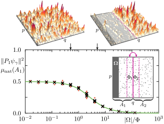
Figure 1: (color online) Weight $\|P_{1}\psi_{\gamma}\|^{2}$ (symbols) of resonance states in region $A_{1}$ vs ratio of size $|\Omega|$ of opening and flux $\Phi$ across a partial barrier for different parameters of the partial-barrier standard map ($16\leq\Phi/h,|\Omega|/h\leq 2048$; $|A_{1}|=0.5$; $h=1/6000$). Weight of state with $\gamma$ closest to $\gamma_{\text{nat}}$ (red points) and averaged over states with decay rates $\gamma\in[\gamma_{\text{nat}}/1.1,1.1\,\gamma_{\text{nat}}]$ (black crosses). This is compared to the natural CIM $\mu_{\text{nat}}(A_{1})$ [Eq. (4), solid green line]. Inset: Phase space of the partial-barrier map, illustrating regions $A_{1}$, $A_{2}$ on either side of the partial barrier (solid magenta line) with exchanging regions $\Phi_{1}$, $\Phi_{2}$, and opening $\Omega$. Upper panels: Husimi representation of typical resonance states with $\gamma\approx\gamma_{\text{nat}}$ for $h=1/1000$, $\Phi/h=20$, and two values $|\Omega|/\Phi$ indicated by arrows.

Since the localization appears in a semiclassical regime ($h\ll\Phi$), one may wonder if it has a classical origin. Thus one needs the classical counterpart of a quantum resonance state. This is given in the field of open dynamical systems Pianigiani and Yorke (1979); Kantz and Grassberger (1985); Tél (1987); Demers and Young (2006); Nonnenmacher and Rubin (2007); Lai and Tél (2011); Altmann et al. (2013a, b); Motter et al. (2013) by a conditionally invariant measure (CIM). It is invariant under time evolution up to an exponential decay with rate $\gamma$. The asymptotic decay of generic initial phase-space distributions leads to the so-called natural CIM $\mu_{\text{nat}}$ with decay rate $\gamma_{\text{nat}}$. The quantum-mechanical relevance of $\mu_{\text{nat}}$ is shown in Casati et al. (1999); Lee et al. (2004); Nonnenmacher and Rubin (2007); Novaes (2013); Altmann et al. (2013a). Note that the steady probability distribution introduced in the context of optical microcavities Lee et al. (2004) corresponds to $\mu_{\text{nat}}$. The natural CIM $\mu_{\text{nat}}$ for the single decay rate $\gamma_{\text{nat}}$, however, cannot be the classical counterpart for all quantum resonance states as they have a wide range of decay rates (see, e.g., Fig. 2). Exceptional CIMs with decay rate $\gamma$ different from $\gamma_{\text{nat}}$ have been discussed Demers and Young (2006); Nonnenmacher and Rubin (2007). In fact, for each $\gamma$ one can construct infinitely many CIMs. It is an open question which of these CIMs correspond to quantum resonance states for arbitrary $\gamma$. To answer this question one has to go beyond the important results of Ref. Keating et al. (2006) which relate the total weight of a resonance state on each forward escaping set to its decay rate.

In this Letter, we introduce the quantum mechanically relevant class of CIMs. Their localization explains the localization of chaotic resonance states in the presence of a partial barrier. In particular, we find (i) a transition from equipartition to localization when opening the system, Fig. 1, and (ii) a transition from localization on one side of the partial barrier to localization on the other side for resonance states with increasing decay rate, Fig. 2. We numerically demonstrate quantum-to-classical correspondence for a designed partial-barrier map and the generic standard map.

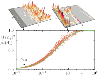
Figure 2: (color online) Weight $\|P_{1}\psi_{\gamma}\|^{2}$ (red points) of resonance states $\psi_{\gamma}$ in region $A_{1}$ vs decay rate $\gamma$ for the partial-barrier standard map ($\Phi/h=64$; $|\Omega|/h=1024$; $|A_{1}|=0.5$; $h=1/6000$). This is compared to the $\gamma$-natural CIM $\mu_{\gamma}(A_{1})$ [Eq. (4), solid green line]. Upper panels: Husimi representation of typical long-lived (left) and short-lived (right) resonance state for $h=1/1000$ with $\gamma$ values indicated by arrows.

Partial-barrier map.—We design a chaotic model map with a single partial barrier (similar to Ref. Körber et al. (2013)), which allows for numerically varying the flux across the partial barrier and for deriving the classical localization, Eq. (4). The partial-barrier map $T=M\circ E\circ O$ is a composition of three maps: the map $M$ describes the unconnected chaotic dynamics within two regions, $A_{k}$. They decompose the phase space $\Gamma=[0,1)\times[0,1)$ into $A_{1}=[0,|A_{1}|)\times[0,1)$ and its complement $A_{2}=\Gamma\setminus A_{1}$; see the inset in Fig. 1, where $|A_{1}|$ denotes the area of $A_{1}$ and by normalization, $|A_{2}|=1-|A_{1}|$. The map $E$ induces a flux $\Phi$ between $A_{1}$ and $A_{2}$ by exchanging regions $\Phi_{k}\subset A_{k}$ with $|\Phi_{k}|=\Phi$. The map $O$ opens the system by the absorbing region $\Omega$, which is contained in region $A_{1}$.

We introduce two different dynamics for $M$. For the numerical analysis, we use the generic standard map Casati et al. (1979) on the torus in symmetrized form, $q_{t+1}=q_{t}+p_{t}^{*}$, $p_{t+1}=p_{t}^{*}+v(q_{t+1})$ with $p_{t}^{*}=p_{t}+v(q_{t})$ for $v(q)=\frac{\kappa}{4\pi}\sin(2\pi q)$ acting individually on each of the regions $A_{k}$ after appropriate rescaling. We fix $\kappa=10$ where the standard map displays a fully chaotic phase space. For analytical considerations, we use the ternary Baker map in each region $A_{k}$, as illustrated in Fig. 3(a), which allows for the derivation of Eq. (4). We refer to the corresponding maps $T$ as partial-barrier standard map and partial-barrier Baker map, respectively.

Quantum localization transitions.—Let us consider the quantization $U$ of the partial-barrier standard map $T$. From the eigenvalue problem for $U$,

$$U\psi_{\gamma}=e^{-\gamma/2}e^{i\theta}\psi_{\gamma},$$ (1)

we numerically compute the decay rates $\gamma$, describing the temporal decay of the norm, $\|U^{t}\psi_{\gamma}\|^{2}=e^{-\gamma t}$, and the corresponding resonance states $\psi_{\gamma}$ (the phase $\theta$ is not relevant in the following). The absolute weight of $\psi_{\gamma}$ in region $A_{1}$ is given by $\|P_{1}\psi_{\gamma}\|^{2}$, where $P_{1}$ denotes the projection onto the subspace associated to $A_{1}$. We observe (i) a transition from equipartition to localization on $A_{2}$ for increasing size $|\Omega|$ of the opening, see Fig. 1, and (ii) a transition from localization on $A_{2}$ to localization on $A_{1}$ for increasing $\gamma$, see Fig. 2. Transition (i) is surprising as localization occurs for $h\ll\Phi$, where in the closed system all eigenstates are equipartitioned Michler et al. (2012). Transition (ii) shows that in open systems the localization depends on the decay rate $\gamma$.

In Fig. 1, we focus on resonances with decay rate $\gamma\approx\gamma_{\text{nat}}$, which describes the decay of typical long-lived resonance states in the semiclassical limit. We find transition (i) from equipartition, $\|P_{1}\psi_{\gamma}\|^{2}=|A_{1}|$, for $|\Omega|\ll\Phi$ to localization on $A_{2}$ for $|\Omega|\gg\Phi$ for various values of $\Phi/h$ and $|\Omega|/h$. The transition is universal with the scaling parameter $|\Omega|/\Phi$. Moreover, this even holds for individual states without averaging (red dots). We stress that this localization transition in the open system occurs even though $\Phi/h\geq 10$, where in the closed system all eigenstates are equipartitioned Michler et al. (2012).

In Fig. 2, we fix the parameters such that $|\Omega|\gg\Phi$, for which the long-lived resonance states localize on $A_{2}$, and show the $\gamma$ dependence of the weights $\|P_{1}\psi_{\gamma}\|^{2}$ for all resonance states. We find transition (ii) from resonance states which localize on $A_{2}$ for small $\gamma$ to resonance states which localize on $A_{1}$ for large $\gamma$, including equipartitioned resonance states in between.

The fact that both transitions (i) and (ii) occur for $h\ll\Phi$ suggests that the localization transitions could be of classical origin. Furthermore, from the point of view of decaying classical distributions the observed transitions qualitatively seem to be rather intuitive: in Fig. 1, for a larger size of the opening one has less weight in region $A_{1}$. In Fig. 2, a larger weight in $A_{1}$ corresponds to a larger decay rate. For a quantitative description, however, one needs to find the quantum mechanically relevant class of CIMs.

Classical localization.—A conditionally invariant measure (CIM) $\mu_{\gamma}$ is defined by

$$\mu_{\gamma}(T^{-1}(X))=e^{-\gamma}\mu_{\gamma}(X),$$ (2)

for each measurable subset $X$ of phase space. It is invariant under the classical iterative dynamics $T$ of the open system up to an exponential decay with rate $\gamma$. Equation (2) states that the measure $\mu_{\gamma}(T^{-1}(X))$ of the set $T^{-1}(X)$ that will be mapped to $X$ is smaller than $\mu_{\gamma}(X)$ by the factor $e^{-\gamma}$. These measures must be zero on the iterates of the opening $\Omega$. Thus, the support of $\mu_{\gamma}$ is the fractal backward trapped set $\Gamma_{\text{b}}$ [horizontal black stripes in Fig. 3(b)], that is the set of points in phase space which do not escape under backward time evolution. Particularly important is the natural CIM $\mu_{\text{nat}}$, see Fig. 3(c), which is constant on its support [because of integration over boxes in Fig. 3(c) one finds two nonzero box measures].

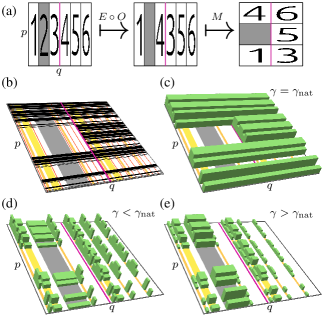
Figure 3: (color online) (a) Illustration of the partial-barrier Baker map $T=M\circ E\circ O$. Magenta line indicates partial barrier and gray shaded region marks the opening (left and central) and image of opening (right). (b) Backward trapped set (dark horizontal stripes) and forward escaping sets $\Omega$ (gray), $T^{-1}(\Omega)$ (yellow), $T^{-2}(\Omega)$ (orange), and $T^{-3}(\Omega)$ (red). (c) Natural CIM integrated over boxes of size $3^{-3}$ in the $p$ direction. (d), (e) Approximation of $\gamma$-natural CIMs by truncation of Eq. (3) to $n\leq 2$ for $\gamma\neq\gamma_{\text{nat}}$.

We now generalize $\mu_{\text{nat}}$ to a CIM $\mu_{\gamma}$ of arbitrary decay rate $\gamma$, which we call $\gamma$-natural CIM. To this end, we use a construction of CIMs Demers and Young (2006); Nonnenmacher and Rubin (2007) where one starts with an arbitrary probability measure on the intersection $\Omega\cap\Gamma_{\text{b}}$ of the opening $\Omega$ with the backward trapped set $\Gamma_{\text{b}}$. By propagating this measure backwards to all forward escaping sets $T^{-n}(\Omega)$ [vertical colored stripes in Fig. 3(b)] and appropriate scaling [respecting the decay rate $\gamma$, Eq. (2)] one obtains a CIM. Here, we choose the simplest measure on $\Omega\cap\Gamma_{\text{b}}$, given by $\mu_{\text{nat}}$. This choice of a measure, which is constant on its support, is quantum mechanically motivated in analogy to quantum ergodicity for closed fully chaotic systems, where eigenstates in the semiclassical limit approach the constant invariant measure Bäcker et al. (1998); Degli Esposti and Graffi (2003). This choice leads to the $\gamma$-natural CIM

$$\mu_{\gamma}(X)=\mathcal{N}\,\sum_{n=0}^{\infty}e^{(\gamma_{\text{nat}}-\gamma)n}\mu_{\text{nat}}(X\cap T^{-n}(\Omega)),$$ (3)

with normalization $\mathcal{N}=(1-e^{-\gamma})/(1-e^{-\gamma_{\text{nat}}})$. This series multiplies $\mu_{\text{nat}}$ in each forward escaping set $T^{-n}(\Omega)$ by an appropriate factor which imposes the overall decay rate $\gamma$ according to Eq. (2). Two examples of $\gamma$-natural CIMs for the partial-barrier Baker map are shown in Figs. 3(d) and 3(e). The measure is constant on $T^{-n}(\Omega)\cap\Gamma_{\text{b}}$ for each $n\in\mathbbm{N}_{0}$. With increasing $n$, this constant is decreasing (increasing) for $\gamma>\gamma_{\text{nat}}$ ($\gamma<\gamma_{\text{nat}}$); in particular, short-lived measures $\mu_{\gamma}$ have more weight in the opening. Note that the idea underlying Eq. (3) was used without the notion of CIMs in Ref. Keating et al. (2006) for sets $X=T^{-n}(\Omega)$ for systems without a partial barrier. Moreover, note that the $\gamma$-natural CIMs are solutions of the exact Perron–Frobenius operator (which is not available), but cannot be obtained from finite-dimensional approximations. Therefore, they have to be constructed directly in phase space.

We find as our main result on the classical localization of $\mu_{\gamma}$ due to a partial barrier that the weight of $\mu_{\gamma}$ on each side of the partial barrier is given by 

$$\mu_{\gamma}(A_{1})=\frac{\mu_{\text{nat}}(A_{1})-c_{\gamma}}{1-c_{\gamma}},$$ (4)

and $\mu_{\gamma}(A_{2})=1-\mu_{\gamma}(A_{1})$, with

$$c_{\gamma}=\left(1-e^{\gamma-\gamma_{\text{nat}}}\right)\,\left(1-e^{-\gamma_{\text{nat}}}\right)\,\frac{|A_{1}|}{|\Omega|}\frac{|A_{2}|}{\Phi}.$$ (5)

The values for $\mu_{\text{nat}}(A_{1})$ and $\gamma_{\text{nat}}$ follow from the longest-lived eigenstate of the eigenvalue problem

$$F_{\text{nat}}\begin{pmatrix}\mu_{\text{nat}}(A_{1})\\ \mu_{\text{nat}}(A_{2})\end{pmatrix}=e^{-\gamma_{\text{nat}}}\begin{pmatrix}\mu_{\text{nat}}(A_{1})\\ \mu_{\text{nat}}(A_{2})\end{pmatrix},$$ (6)

where $F_{\text{nat}}$ denotes the transition matrix between $A_{1}$ and $A_{2}$ for the one-step propagation of $\mu_{\text{nat}}$ (see Ref. Weber et al. (2001) for approximations of the Perron–Frobenius operator). In general, $F_{\text{nat}}$ may be obtained numerically or it may be approximated by assuming a uniform distribution for $\mu_{\text{nat}}$,

$$F_{\text{nat}}\approx\begin{pmatrix}1-(|\Omega|+\Phi)/|A_{1}|&\Phi/|A_{2}|\\ \Phi/|A_{1}|&1-\Phi/|A_{2}|\end{pmatrix}.$$ (7)

This turns out to be quite a good approximation even for fractal $\mu_{\text{nat}}$ and it is exact for the partial-barrier Baker map.

Quantum-to-classical correspondence.—Figure 1 (green line) shows the classical localization $\mu_{\gamma}(A_{1})$, Eq. (4), for $\gamma=\gamma_{\text{nat}}$ (i.e., $c_{\gamma}=0$ and $\mu_{\gamma}=\mu_{\text{nat}}$), using the approximation Eq. (7). When increasing the size $|\Omega|$ of the opening, we find a transition from equipartition for $|\Omega|\ll\Phi$ to localization for $|\Omega|\gg\Phi$. The only scaling parameters are $|\Omega|/\Phi$ and $|A_{1}|/|A_{2}|$. We find very good agreement of the classical localization measure with the localization of the quantum resonance states. Note that for $\gamma\neq\gamma_{\text{nat}}$, the localization depends on all parameters $|\Omega|$, $\Phi$, and $|A_{1}|$.

Figure 2 (green line) shows Eq. (4) as a function of $\gamma$. The classical localization measure $\mu_{\gamma}(A_{1})$ monotonically increases with $\gamma$; i.e., the faster the decay, the larger is the weight in region $A_{1}$ with the opening $\Omega$. In the limit $\gamma\to\infty$ one finds $\mu_{\gamma}(A_{1})=1$, and in fact, all the weight is in the opening $\Omega$. In the limit $\gamma\to 0$ one finds a small constant $\mu_{0}(A_{1})>0$; i.e., even though most of the weight is in $A_{2}$ there is always a small contribution in $A_{1}$ due to the exchange between $A_{1}$ and $A_{2}$. Again, we find very good agreement between the classical localization measure and the localization of the quantum resonance states for all decay rates $\gamma$. Note that quantum-to-classical correspondence is also confirmed for $|A_{1}|\neq|A_{2}|$ (not shown).

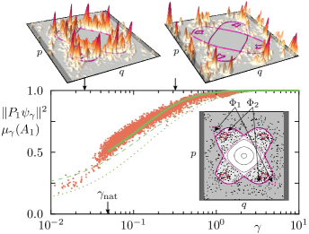
Figure 4: (color online) Weight $\|P_{1}\psi_{\gamma}\|^{2}$ (red points) of resonance states $\psi_{\gamma}$ in region $A_{1}$ vs decay rate $\gamma$ for standard map at $\kappa=2.9$, with $|A_{1}|\approx 0.6664$, $|A_{2}|\approx 0.2061$, $\Phi\approx 0.0126$, $|\Omega|=0.1$, and $h=1/10000$. This is compared to the $\gamma$-natural CIM $\mu_{\gamma}(A_{1})$, either by direct numerical computation Note (1) (solid green line), using Eq. (4) and computing $F_{\text{nat}}$ numerically (dashed green line), or by using approximation Eq. (7) (dotted green line). Inset: Phase space of the standard map with regular and chaotic regions, illustrating regions $A_{1}$ (medium gray shaded), $A_{2}$ (light gray shaded) on either side of the main partial barrier (thick solid magenta line) with exchanging regions $\Phi_{1}$, $\Phi_{2}$, and opening $\Omega$ (dark gray shaded). Upper panels: Husimi representation of typical long-lived (left) and short-lived (right) resonance states for $h=1/1000$ with $\gamma$ values indicated by arrows.

Do these results for the partial-barrier map generalize to generic systems? In Fig. 4, we show for the standard map at $\kappa=2.9$, where it has a mixed phase space, that the localization of the chaotic resonance states on region $A_{1}$, which contains the opening, increases as a function of $\gamma$. Qualitatively, we find the same localization behavior as for the partial-barrier standard map in Fig. 2. Quantitatively, it is well described by the classical localization of $\mu_{\gamma}$, which is determined numerically Note (1). Also the analytical prediction, Eq. (4), works reasonably well. Overall, Figs. 1, 2, and 4 demonstrate quantum-to-classical correspondence for the localization of chaotic resonance states in open systems due to a partial barrier.

Outlook.—We see the following future challenges: (a) While in this work we concentrate on the weights on either side of a partial barrier one should verify the quantum-to-classical correspondence for the fine-structure of chaotic resonance states to $\gamma$-natural CIMs. (b) Which deviations arise when approaching the quantum regime of $h\approx\Phi$, $|\Omega|$? (c) Is the new class of $\gamma$-natural CIMs, which is quantum mechanically motivated, of relevance also in classical dynamical systems? (d) Is it possible to predict which quantum mechanical decay rates $\gamma$ occur in the presence of a partial barrier including their distribution, as it is known for fully chaotic systems Życzkowski and Sommers (2000); Nonnenmacher and Zworski (2009); Micklitz and Altland (2013)? (e) The present work explains the localization of resonance states which have been used to derive the hierarchical fractal Weyl laws Körber et al. (2013) for a hierarchy of partial barriers. Now it is possible to discuss whether these laws survive in the semiclassical limit. (f) We see direct applications to mode coupling in optical microcavities Wiersig (2014) and in recently studied parity–time symmetric systems West et al. (2010); Schomerus (2013), where instead of a partial barrier one has coupled symmetry-related subspaces.

I Supplemental Material

Classical derivation.—In order to derive Eq. (4), we focus on the localization properties of $\mu_{\gamma}$ with respect to the partial barrier, restricting ourselves to the partial-barrier Baker map in the following. The generalization to other systems will be discussed at the end.

The localization of $\mu_{\gamma}$ is described by its weights $\mu_{\gamma}(A_{k})$ on either side of the partial barrier. In virtue of Eq. (3), we only have to study $\mu_{\text{nat}}(A_{k}\cap T^{-n}(\Omega))$ in more detail to compute $\mu_{\gamma}(A_{k})$. We find that the natural measure of $A_{k}\cap T^{-n}(\Omega)$ is proportional to its relative area inside $A_{k}$,

$$\mu_{\text{nat}}(A_{k}\cap T^{-n}(\Omega))=\mu_{\text{nat}}(A_{k})\cdot\frac{|A_{k}\cap T^{-n}(\Omega)|}{|A_{k}|}.$$ (S1)

This follows from the fact that the forward escaping sets $T^{-n}(\Omega)$ decompose the backward trapped set $\Gamma_{\text{b}}$ in the unstable (horizontal) direction, on which $\mu_{\text{nat}}$ is uniformly distributed within $A_{1}$ and $A_{2}$ individually, see Fig. 3(c).

The distribution of the opening $\Omega$ over phase space under backward time evolution, which enters Eq. (S1) in terms of $|A_{k}\cap T^{-n}(\Omega)|$, follows from

$$\begin{pmatrix}|A_{1}\cap T^{-n}(\Omega)|\\ |A_{2}\cap T^{-n}(\Omega)|\end{pmatrix}=F_{\text{nat}}^{n}\begin{pmatrix}|\Omega|\\ 0\end{pmatrix},$$ (S2)

where $F_{\text{nat}}$ denotes the transition matrix between $A_{1}$ and $A_{2}$ for the one-step propagation of $\mu_{\text{nat}}$. Note that the transition matrix for the backward time evolution of $\Omega$ is given by $F_{\text{nat}}$ itself. This relation can be interpreted using Fig. 3(b): In the beginning, $\Omega$ (gray vertical stripe) is supported on $A_{1}$. In the next step, $T^{-1}(\Omega)$ (yellow) splits into equal parts on $A_{1}$ and $A_{2}$. Afterwards, $T^{-2}(\Omega)$ (orange) contributes two stripes to $A_{1}$ and three to $A_{2}$.

Inserting the relations (S1) and (S2) in Eq. (3), and using Neumann’s series, we obtain

$$\mu_{\gamma}(A_{k})=\mathcal{N}\frac{\mu_{\text{nat}}(A_{k})}{|A_{k}|}\left[\bigl{(}\mathbbm{1}-e^{\gamma_{\text{nat}}-\gamma}F_{\text{nat}}\bigr{)}^{-1}\begin{pmatrix}|\Omega|\\ 0\end{pmatrix}\right]_{k}.$$ (S3)

Our result on the classical localization, Eq. (4), follows from Eq. (S3) after some algebra.

We believe that this derivation for the partial-barrier Baker map can be generalized to generic dynamical systems. This is indicated by the numerical findings for the partial-barrier standard map, Fig. 2, as well as the standard map, Fig. 4, compared to Eq. (4). The main reason for the deviations of Eq. (4) for a generic system is that Eq. (S1) is not valid in general. For its generalization, one has to revise the argument in the natural coordinates of the stable and unstable manifolds.

Standard map.—In the following, we explain how to determine $\mu_{\gamma}$ for a generic system like the standard map numerically. First, one has to approximate (the chaotic part of) the backward trapped set $\Gamma_{\text{b}}$. To this end, one may define a uniform grid of $N_{\text{grid}}$ points in phase space of which one has to discard points which leave the system within $N_{\text{iter}}$ iterations of the map $T$ in backward time direction. For Fig. 4, we choose $N_{\text{grid}}=10^{6}$ and $N_{\text{iter}}=50$. Points within a regular phase-space region should be omitted manually. The remaining points provide the finite-time approximation $\Gamma_{\text{b}}^{\text{num}}$ of $\Gamma_{\text{b}}$ and need to be classified by their forward escaping times. Following Ref. [18], we associate the $\mu_{\gamma}$ measure $e^{-\gamma n}(1-e^{-\gamma})$ to set $T^{-n}(\Omega)\cap\Gamma_{\text{b}}^{\text{num}}$. Finally, assuming equidistribution for the points in $T^{-n}(\Omega)\cap\Gamma_{\text{b}}^{\text{num}}$, we find

$$\mu_{\gamma}(X\cap T^{-n}(\Omega))\approx f_{n}(X)\,e^{-\gamma n}(1-e^{-\gamma}),$$ (S4)

for each (measurable) subset $X$ of phase space and

$$f_{n}(X):=\frac{\#\left(X\cap T^{-n}(\Omega)\cap\Gamma_{\text{b}}^{\text{num}}\right)}{\#\left(T^{-n}(\Omega)\cap\Gamma_{\text{b}}^{\text{num}}\right)}$$ (S5)

where $\#$ denotes the cardinality of a set. Using $\mu_{\gamma}(X)=\sum_{n=0}^{\infty}\mu_{\gamma}(X\cap T^{-n}(\Omega))$ we have a numerical estimate for the $\gamma$-natural CIM $\mu_{\gamma}$. As the sample $\Gamma_{\text{b}}^{\text{num}}$ is only finite the series will terminate and the numerically approximated measure is not perfectly normalized. This method is not appropriate for exceedingly small $\gamma$ since the weight on forward escaping sets $T^{-n}(\Omega)\cap\Gamma_{\text{b}}^{\text{num}}$ with large escape times $n$ increases while they are approximated by a few points only. Hence, we restrict the method to $\gamma\geq\gamma_{\text{nat}}$ in Fig. 4.

Quantum mechanically, owing to the mixed phase space of a generic system, we discard all regular and deeper hierarchical states having less than 50% of their weight within $A_{1}$ and $A_{2}$. As some of the remaining chaotic resonance states still have a significant contribution outside of $A_{1}\cup A_{2}$, we renormalize them such that $\|P_{1}\psi_{\gamma}\|^{2}+\|P_{2}\psi_{\gamma}\|^{2}=1$.