TMB: Automatic Differentiation and Laplace Approximation

Kasper Kristensen, Anders Nielsen, Casper W. Berg, Hans Skaug, Brad Bell TMB: Automatic Differentiation and Laplace Approximation TMB: Template Model Builder TMB is an open source R package that enables quick implementation of complex nonlinear random effect (latent variable) models in a manner similar to the established AD Model Builder package (ADMB, admb-project.org) (Fournier et al., 2011). In addition, it offers easy access to parallel computations. The user defines the joint likelihood for the data and the random effects as a C++ template function, while all the other operations are done in R; e.g., reading in the data. The package evaluates and maximizes the Laplace approximation of the marginal likelihood where the random effects are automatically integrated out. This approximation, and its derivatives, are obtained using automatic differentiation (up to order three) of the joint likelihood. The computations are designed to be fast for problems with many random effects ($\approx 10^{6}$) and parameters ($\approx 10^{3}$). Computation times using ADMB and TMB are compared on a suite of examples ranging from simple models to large spatial models where the random effects are a Gaussian random field. Speedups ranging from 1.5 to about 100 are obtained with increasing gains for large problems. The package and examples are available at http://tmb-project.org. automatic differentiation, AD, random effects, latent variables, C++ templates, R automatic differentiation, AD, random effects, latent variables, C++ templates, R Kasper Kristensen
DTU Compute
Matematiktorvet
Building 303 B
DK-2800 Kgs. Lyngby
E-mail:
URL: http://imm.dtu.dk/~kaskr/ Submitted to Journal of Statistical Software

1 Introduction

Calculation of derivatives plays an important role in computational statistics. One classic application is optimizing an objective function; e.g., maximum likelihood. Given a computer algorithm that computes a function, Automatic Differentiation (AD) (Griewank and Walther, 2008) is a technique that computes derivatives of the function. This frees the statistician from the task of writing, testing, and maintaining derivative code. This technique is gradually finding its way into statistical software; e.g., the C++ packages ADMB (Fournier et al., 2011), Stan (Stan Development Team, 2013) and Ceres Solver (Agarwal and Mierle, 2013). These packages implement AD from first principles, rather than using one of the general purpose AD packages that are available for major programming languages such as Fortran, C++, Python, and MATLAB (Bücker and Hovland, 2014). The Template Model Builder (TMB) R package uses CppAD (Bell, 2005) to evaluate first, second, and possibly third order derivatives of a user function written in C++. Maximization of the likelihood, or a Laplace approximation for the marginal likelihood, is performed using conventional R optimization routines. The numerical linear algebra library Eigen (Guennebaud et al., 2010) is used for C++ vector and matrix operations. Seamless integration of CppAD and Eigen is made possible through the use of C++ templates.

First order derivatives are usually sufficient for maximum likelihood and for hybrid MCMC; e.g., the Stan package which provides both only uses first order derivatives (Stan Development Team, 2013). Higher order derivatives calculated using AD greatly facilitate optimization of the Laplace approximation for the marginal likelihood in complex models with random effects; e.g., Skaug and Fournier (2006). This approach, implemented in ADMB and TMB packages, has been used to fit simple random effect models as well as models containing Gaussian Markov random fields (GMRF). In this paper, we compare computation times between these two packages for a range of random effects models.

Many statisticians are unfamiliar with AD and for those we recommend reading sections 2.1 and 2.2 of Fournier et al. (2011). The ADMB package is rapidly gaining new users due to its superiority with respect to optimization speed and robustness (Bolker et al., 2013) compared to e.g. winBUGS (Spiegelhalter et al., 2003). The TMB package is built around the same principles, but rather than being coded more or less from scratch, it combines several existing high-performance libraries, to be specific, CppAD for automatic differentiation in C++, Matrix for sparse and dense matrix calculations in R, Eigen for sparse and dense matrix calculations in C++, and OpenMP for parallelization in C++ and Fortran. Using these packages yields better performance and a simpler code-base making TMB easy to maintain.

The conditional independence structure in state-space models and GMRFs yields a sparse precision matrix for the joint distribution of the data and the random effects. It is well known that, when this precision matrix is sparse, it is possible to perform the Laplace approximation for models with a very large number of random effects; e.g., INLA (Rue et al., 2009). The INLA package (http://www.r-inla.org/download) restricts the models to cases where the sparseness structure is known a priori and models can be written in one line of R code. In contrast ADMB requires manual identification of conditional independent likelihood contributions, but is not restricted to any special model class. The TMB package can fit the same models as ADMB, but is better equipped to take maximal advantage of sparseness structure. It uses an algorithm to automatically determine the sparsity structure. Furthermore, in situations where the likelihood can be factored, it enables parallelization using OpenMP (Dagum and Menon, 1998). It also allows parallelization through BLAS (Dongarra et al., 1990) during Cholesky factorization of large sparse precision matrices. (Note that the BLAS library is written in Fortran.)

C++ templates treat variable types as parameters. This obtains the advantages of loose typing because one code base can work on multiple types. It also obtains the advantage of strong typing because types are checked at compile time and the code is optimized for the particular type. CppAD’s use of templates enables derivatives calculations to be recorded and define other functions that can then be differentiated. Eigen’s use of templates enables matrix calculations where corresponding scalar types can do automatic differentiation. These features are important in the implementation and use of TMB.

The rest of this paper is organized as follows: Section 2 is a review of the Laplace approximation for random effects models. Section 3 is a review of automatic differentiation as it applies to this paper. Section 4 describes how TMB is implemented. Section 5 describes the package from a user’s perspective. Section 6 compares its performance with that of ADMB for a range of models where the number of parameters is between $1$ and $16$ and the number of random effects is between $40$ and $40,000$. Section 7 contains a discussion and conclusion.

2 The Laplace Approximation

The statistical framework in this section closely follows that of Skaug and Fournier (2006). Let $f(u,\theta)$ denote the negative joint log-likelihood of the data and the random effects. This depends on the unknown random effects $u\in\mathbb{R}^{n}$ and parameters $\theta\in\mathbb{R}^{m}$. The data, be it continuous or discrete, is not made explicit here because it is a known constant for the analysis in this section. The function $f(u,\theta)$ is provided by the TMB user in the form of C++ source code. The range of applications is large, encompassing all random effects models for which the Laplace approximation is appropriate.

The TMB package implements maximum likelihood estimation and uncertainty calculations for $\theta$ and $u$. It does this in an efficient manner and with minimal effort on the part of the user. The maximum likelihood estimate for $\theta$ maximizes

$$L(\theta)=\int_{\mathbb{R}^{n}}\exp(-f(u,\theta))\>du$$

w.r.t. $\theta$. Note that the random effects $u$ have been integrated out and the marginal likelihood $L(\theta)$ is the likelihood of the data as a function of just the parameters. We use $\hat{u}(\theta)$ to denote the minimizer of $f(u,\theta)$ w.r.t. $u$; i.e.,

$$\hat{u}(\theta)=\arg\min_{u}f(u,\theta)\;.$$ (1)

We use $H(\theta)$ to denote the Hessian of $f(u,\theta)$ w.r.t. $u$ and evaluated at $\hat{u}(\theta)$; i.e.,

$$H(\theta)=f^{\prime\prime}_{uu}(\hat{u}(\theta),\theta)\;.$$ (2)

The Laplace approximation for the marginal likelihood $L(\theta)$ is

$$L^{*}(\theta)=\sqrt{2\pi}^{n}\det(H(\theta))^{-\frac{1}{2}}\exp(-f(\hat{u},\theta))\;.$$ (3)

This approximation is widely applicable including models ranging from non-linear mixed effects models to complex space-time models. Certain regularity conditions on the joint negative log-likelihood function are required; e.g., the minimizer of $f(u,\theta)$ w.r.t. $u$ is unique. These conditions are not discussed in this paper.

Models without random effects ($n=0$), and models for which the random effects must be integrated out using classical numerical quadratures, are outside the focus of this paper.

Our estimate of $\theta$ minimizes the negative log of the Laplace approximation; i.e.,

$$-\log L^{*}(\theta)=-n\log\sqrt{2\pi}+\frac{1}{2}\log\det(H(\theta))+f(\hat{u},\theta).$$ (4)

This objective and its derivatives are required so that we can apply standard nonlinear optimization algorithms (e.g., BFGS) to optimize the objective and obtain our estimate for $\theta$. Uncertainty of the estimate $\hat{\theta}$, or any differentiable function of the estimate $\phi(\hat{\theta})$, is obtained by the $\delta$-method:

$$\VAR(\phi(\hat{\theta}))=-\phi^{\prime}_{\theta}(\hat{\theta})\left(\nabla^{2}\log L^{*}(\hat{\theta})\right)^{-1}\phi^{\prime}_{\theta}(\hat{\theta})^{\top}.$$ (5)

A generalized version of this formula is used to include cases where $\phi$ also depends on the random effects, i.e. $\phi(u,\theta)$, (Skaug and Fournier, 2006; Kass and Steffey, 1989). These uncertainty calculations also require derivatives of (4). However, derivatives are not straight-forward to obtain using automatic differentiation in this context. Firstly, because $\hat{u}$ depends on $\theta$ indirectly as the solution of an inner optimization problem; see (1). Secondly, equation (4) involves a log determinant, which is found through a Cholesky decomposition. A naive application of AD, that ignores sparsity, would tape on the order of $n^{3}$ floating point operations. While some AD packages would not record the zero multiplies and adds, they would still take time to detect these cases. TMB handles these challenges using state-of-the-art techniques and software packages. In the next section, we review its use of the CppAD package for automatic differentiation.

3 AD and CppAD

Given a computer algorithm that defines a function, Automatic Differentiation (AD) can be used to compute derivatives of the function. We only give a brief overview of AD, and refer the reader to Griewank and Walther (2008) for a more in-depth discussion. There are two different approaches to AD: “source transformation" and “operator overloading". In source transformation; e.g., the package TAPENADE (Hascoet and Pascual, 2004), a preprocessor generates derivative code that is compiled together with the original program. This approach has the advantage that all the calculations are done in compiler native floating point type (e.g., double-precision) which tends to be faster than AD floating point types. In addition the compiler can apply its suite of optimization tricks to the derivative code. Hence source transformation tends to yield the best run time performance, both in terms of speed and memory use.

In the operator overloading approach to AD, floating point operators and elementary functions are overloaded using types that perform AD techniques at run time. This approach is easier to implement and to use because it is not necessary to compile and interface to extra automatically generated source code each time an algorithm changes. ADOL-C (Walther and Griewank, 2012) and CppAD (Bell, 2005) implement this approach using the operator overloading features of C++. Because TMB uses CppAD it follows that its derivative calculations are based on the operator overloading approach.

During evaluation of a user’s algorithm, CppAD builds a representation of the corresponding function, often referred to as a “tape" or the “computational graph". Figure 1 shows a graphical representation of T1, the tape for the example function $f:\mathbb{R}^{8}\rightarrow\mathbb{R}$, defined by

$$f(\xi_{1},\ldots,\xi_{8})=\xi_{1}^{2}+\sum_{i=2}^{8}(\xi_{i}-\xi_{i-1})^{2}\;.$$

Each node corresponds to a variable, its name is the operation that computes its value, and its number identifies it in the list of all the variables. The initial nodes are the independent variables $\xi_{1},\ldots\xi_{8}$. The final node is the dependent variable corresponding to the function value. There are two main AD algorithms known as the “forward" and “reverse" modes. Forward mode starts with the independent variables and calculates values in the direction of the arrows. Reverse mode does its calculations in the opposite direction.

Because $f$ is a scalar valued function, we can calculate its derivatives with one forward and one reverse pass through the computational graph in Figure 1: Starting with the value for the independent variables nodes 1 through 8, the forward pass calculates the function value for all the other nodes.

The reverse pass, loops through the nodes in the opposite direction. It recursively updates the $k$’th node’s partial derivative $\partial\xi_{24}/\partial\xi_{k}$, given the partials of higher nodes $\partial\xi_{24}/\partial\xi_{i}$, for $i=k+1,...,24$. For instance, to update the partial derivative of node $k=5$, the chain rule is applied along the outgoing edges of node 5; i.e.,

$$\frac{\partial\xi_{24}}{\partial\xi_{5}}=\frac{\partial\xi_{24}}{\partial\xi_{16}}\frac{\partial\xi_{16}}{\partial\xi_{5}}+\frac{\partial\xi_{24}}{\partial\xi_{18}}\frac{\partial\xi_{18}}{\partial\xi_{5}}$$

The partials of the final node, $\partial\xi_{24}/\partial\xi_{16}$ and $\partial\xi_{24}/\partial\xi_{18}$, are available from previous calculations because 16 and 18 are greater than 5. The partials along the outgoing arrows, $\partial\xi_{16}/\partial\xi_{5}$ and $\partial\xi_{18}/\partial\xi_{5}$, are derivatives of elementary operations. In this case, the elementary operation is subtraction and these partials are plus and minus one. (For some elementary operations; e.g., multiplication, the values computed by the forward sweep are needed to compute the partials of the elementary operation.) On completion of the reverse mode loop, the total derivative of $\xi_{24}$ w.r.t. the independent variables is available as $\partial\xi_{24}/\partial\xi_{1}$,…, $\partial\xi_{24}/\partial\xi_{8}$.

For a scalar valued $f$, evaluation of its derivative using reverse mode is surprisingly inexpensive. The number of floating point operations is less than 4 times that for evaluating $f$ itself (Griewank and Walther, 2008). We refer to this as the “cheap gradient principle”. This cost is proportional to the number of nodes in T1; i.e., Figure 1. (The actual result is for a computational graph where there is only one or two arrows into each node. In T1, CppAD combined multiple additions into the final node number 24.) This result does not carry over from scalar valued functions to vector valued functions $g(x)$. It does apply to the scalar-valued inner product $w^{\top}g(x)$, where $w$ is a vector in the range space for $g$. CppAD has provision for using reverse mode to calculate the derivative of $w^{\top}g(x)$ given a range space direction $w$ and a tape for $g(x)$.

CppAD was chosen for AD calculations in TMB because it provides two mechanisms for calculating higher order derivatives. One uses forward and reverse mode of any order. The other is its ability to tape functions that are defined in terms of derivatives and then apply forward and reverse mode to compute derivatives of these functions. We were able to try many different derivative schemes and choose the one that was fastest in our context. To this end, it is useful to tape the reverse mode calculation of $f^{\prime}$ and thereby create the tape T2 in Figure 2. This provides two different ways to evaluate $f^{\prime}$. The new alternative is to apply a zero order forward sweep on T2; i.e., starting with values for nodes 1-8, sequentially evaluate nodes 9-29. On completion the eight components of the vector $f^{\prime}$ are found in the dashed nodes of the graph. If we do a reverse sweep on T2 in the direction $w$, we get

$$\partial_{\xi}[w^{\top}f^{\prime}(\xi)]=\left(\sum_{i=1}^{8}w_{i}\frac{\partial^{2}}{\partial\xi_{1}\partial\xi_{i}}f(x)\;,\;\ldots\;,\;\sum_{i=1}^{8}w_{i}\frac{\partial^{2}}{\partial\xi_{8}\partial\xi_{i}}f(x)\right)$$ (6)

In Section 4 we shall calculate up to third order derivatives using these techniques.

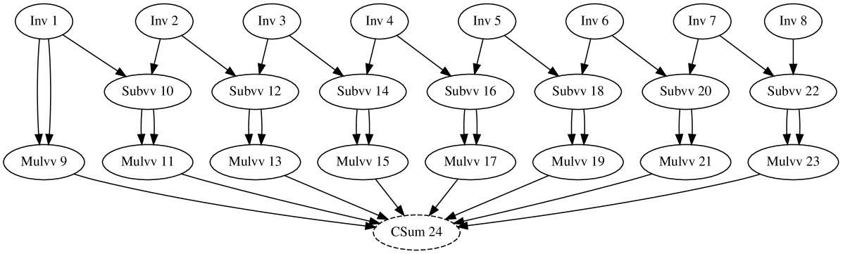
Figure 1: CppAD tape T1 for $f(\xi_{1},\ldots,\xi_{8})=\xi_{1}^{2}+\sum_{i=2}^{8}(\xi_{i}-\xi_{i-1})^{2}\;.$ Nodes “Inv 1"–“Inv 8" correspond to $\xi_{1},\ldots,\xi_{8}$ and node “CSum 24" corresponds to $f(\xi_{1},\ldots,\xi_{8})$. Node labels indicate the elementary operations, numbering indicates the order in these operations are evaluated, arrows point from operation arguments to results, double arrows correspond to the square operator x^2 which is implemented as x*x.

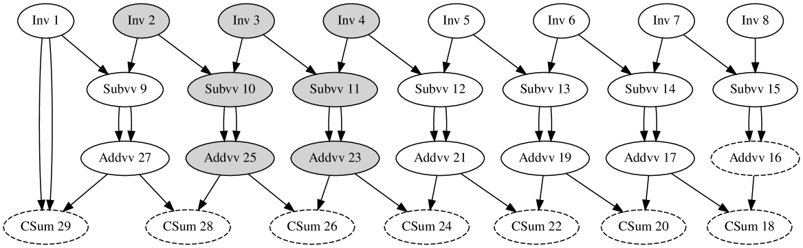
Figure 2: CppAD tape T2 for $f^{\prime}(\xi)$, when $f(\xi)$ is defined as in Figure 1. For example, node 26 corresponds to the partial of $f$ w.r.t. $\xi_{3}$; i.e., $f^{\prime}_{3}(\xi)=2(\xi_{3}-\xi_{2})-2(\xi_{4}-\xi_{3})$. After a zero order forward sweep, $f^{\prime}(\xi)$ is contained in nodes marked with dashed ellipses. Hessian columns of $f$ are found using first order reverse sweeps of T2. For example, to find the 3rd Hessian column it is sufficient to traverse the sub-graph marked in gray; i.e., the nodes that affect the value of node 26.

CppAD does some of its optimization during the taping procedure; e.g., constant expressions are reduced to a single value before being taped. Other optimizations; e.g., removing code that does not affect the dependent variables, can be performed using an option to optimize the tape. This brings the performance of CppAD closer to the source transformation AD tools, especially in cases where the optimized tape is evaluated a large number of times (as is the case with TMB).

4 Software Implementation

TMB calculates estimates of both parameters and random effects using the Laplace approximation (3) for the likelihood. The user provides a C++ function $f(u,\theta)$ that computes the joint likelihood as a function of the parameters $\theta$ and the random effects $u$; see Section 5 for more details. This function, referred to as the “user template" below, defines the user’s statistical model using a standard structure that is expected by the package. Its floating point type is a template parameter so that it can be used with multiple CppAD types. Hence there are two meanings of the use of T (Template) in the package name TMB.

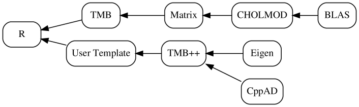
Figure 3: TMB package design: module R is the the top level controlling user code, TMB is the part of TMB that is written in R, Matrix is an R sparse matrix package, CHOLMOD is a C sparse Cholesky factorization routine, BLAS is a Fortran tuned set of basic linear algebra routines, User Template is the user’s joint likelihood in C++, TMB++ is the package components in C++, Eigen is a C++ matrix algebra library, CppAD is a C++ AD package. Arrows indicate package inclusions.

An overview of the package design is shown in Figure 3. Evaluation of the objective $-\log L^{*}(\theta)$ and its derivatives, is performed in R; see equation (4). TMB performs the Laplace approximation with use of CHOLMOD, natively available in R through the Matrix package, and optionally linking to BLAS. Sub-expressions, such as $\hat{u}(\theta)$ and $H(\theta)$, are evaluated in C++. These sub-expressions are returned as R objects, and the interactive nature of R allows the user to easily inspect them. This is important during a model development stage.

Interfaces to the various parts of CppAD constitute a large part of the R code. During an initial phase of program execution the following CppAD tapes are created:

• Tape of $f(u,\theta):\mathbb{R}^{m+n}\rightarrow\mathbb{R}$, generated from user program. Graph size proportional to flop count of user template function.

• Tape of $f^{\prime}(u,\theta):\mathbb{R}^{m+n}\rightarrow\mathbb{R}^{m+n}$, generated from T1 as described in Figure 2. Graph size is at most 4 times the size of T1.

• Tape of $f^{\prime\prime}_{uu}(u,\theta):\mathbb{R}^{m+n}\rightarrow\mathbb{R}^{\ell}$, the $l$ non-zero entries in the lower triangle of $H(\theta)$. Prior to T3’s construction, the sparsity pattern of $H(\theta)$ is calculated by analyzing the dependency structure of T2.

Tapes T1-T3 correspond to Codes 1-3 in Table 1 of Skaug and Fournier (2006). These tapes are computed only once and are subsequently held in memory. The corresponding data structures are part of the R environment and are managed by the R garbage collector just like any other objects created from the R command line.

4.1 Inverse Subset Algorithm

In this section we describe how the tapes T1-T3 are used to calculate the derivative of the objective with respect to the parameters. Define $h:\mathbb{R}^{n+m}\rightarrow\mathbb{R}$ by

$$h(u,\theta)=-\frac{n}{2}\log{2\pi}+\frac{1}{2}\log{\det{f^{\prime\prime}_{uu}(u,\theta)}}+f(u,\theta)\;.$$

It follows that the objective $-\log L^{*}(\theta)$ is equal to $h(\hat{u}(\theta),\theta)$. Furthermore, the function $\hat{u}(\theta)$ satisfies the equations

$$f^{\prime}_{u}(\hat{u}(\theta),\theta) = 0$$

$$\hat{u}^{\prime}(\theta) = -f^{\prime\prime}_{uu}(\hat{u}(\theta),\theta)^{-1}f^{\prime\prime}_{u\theta}(\hat{u}(\theta),\theta).$$

The derivative of the objective w.r.t. $\theta$ is

$$\frac{d}{d\theta}h(\hat{u}(\theta),\theta)=h^{\prime}_{\theta}(\hat{u}(\theta),\theta)-h^{\prime}_{u}(\hat{u}(\theta),\theta)f^{\prime\prime}_{uu}(\hat{u}(\theta),\theta)^{-1}f^{\prime\prime}_{u\theta}(\hat{u}(\theta),\theta).$$ (7)

To simplify the notation, we express $(u,\theta)$ as a single vector $\xi\in\mathbb{R}^{n+m}$. The first step is to evaluate

$$h^{\prime}_{\xi}(\xi)=f^{\prime}_{\xi}(\xi)+\frac{d}{d\xi}\frac{1}{2}\log{\det{f^{\prime\prime}_{uu}(\xi)}}.$$

The term $f^{\prime}_{\xi}(\xi)$ is calculated using a first order reverse sweep on T1. The derivative of the log-determinant is calculated using the well known rule

$$\frac{\partial}{\partial\xi_{i}}\left(\frac{1}{2}\log{\det{f^{\prime\prime}_{uu}(\xi)}}\right)=\frac{1}{2}{\rm tr}\left(f^{\prime\prime}_{uu}(\xi)^{-1}\frac{\partial}{\partial\xi_{i}}f^{\prime\prime}_{uu}(\xi)\right).$$ (8)

The trace of a product of symmetric matrices ${\rm tr}(AB)$ is equal to the sum of the entries of the pointwise product $A\odot B$. Thus, computing the right hand side of equation (8) only requires the elements of $f^{\prime\prime}_{uu}(\xi)^{-1}$ that correspond to non-zero entries in the sparsity pattern for $\partial_{\xi(i)}f^{\prime\prime}_{uu}(\xi)$. The inverse subset algorithm transforms the sparse Cholesky factor $L$ to the inverse $(LL^{\top})^{-1}$ on the sparseness pattern of $LL^{\top}$; e.g., Rue (2005). Let $w\in\mathbb{R}^{\ell}$ denote the elements of $f^{\prime\prime}_{uu}(\xi)^{-1}$ that correspond to non-zeros in the lower triangle of $f^{\prime\prime}_{uu}(\xi)$. We can compute the partial (8), for all $i$, through a single first order reverse sweep of tape T3 in range direction $w$.

Having evaluated $h^{\prime}(\xi)$ we turn to the remaining terms in equation (7). A sparse matrix-vector solve is used to compute

$$v=h^{\prime}_{u}(\hat{u}(\theta),\theta)f^{\prime\prime}_{uu}(\hat{u}(\theta),\theta)^{-1}\;.$$

A reverse mode sweep of tape T2 in range direction $w=(v,0)$ is used to compute

$$\frac{d}{d\xi}[vf^{\prime}_{u}(\hat{u}(\theta),\theta)]=[vf^{\prime\prime}_{uu}(\hat{u}(\theta),\theta),vf^{\prime\prime}_{u\theta}(\hat{u}(\theta),\theta)]\;.$$

This yield the final term needed in equation (7)

$$h^{\prime}_{u}(\hat{u}(\theta),\theta)f^{\prime\prime}_{uu}(\hat{u}(\theta),\theta)^{-1}f^{\prime\prime}_{u\theta}(\hat{u}(\theta),\theta)=vf^{\prime\prime}_{u\theta}(\hat{u}(\theta),\theta)\;.$$

Note that the term $vf^{\prime\prime}_{uu}(\hat{u}(\theta),\theta)$ is not used by the method above. It is necessary to include $u$ in the independent variables for this calculation so that the dependence of $vf^{\prime\prime}_{u\theta}(\hat{u}(\theta),\theta)$ on the value of $\hat{u}(\theta)$ can be included.

Laplace:	$h(\hat{\xi})$	Gradient:	$(d/d\theta)h(\hat{\xi})$
L1: min $f(u,\theta)$ w.r.t. $u$	$\hat{\xi}=(\hat{u},\theta)$
L2: order 0 forward T1	$f(\hat{\xi})$	G1: order 1 reverse T1	$f^{\prime}(\hat{\xi})$
L3: order 0 forward T3	$f^{\prime\prime}_{uu}(\hat{\xi})$	G2: order 1 reverse T3	$\partial_{\xi}f^{\prime\prime}_{uu}(\hat{\xi})$
L4: sparse Cholesky	$LL^{\top}=f^{\prime\prime}_{uu}(\hat{\xi})$	G3: inverse subset	$\partial_{\xi}\log\det f^{\prime\prime}_{uu}(\hat{\xi})$
		G4: sparse solve	$v=h^{\prime}_{u}(\hat{\xi})f_{uu}(\hat{\xi})^{-1}$
		G5: order 0 forward T2	$f^{\prime}(\hat{\xi})$
		G6: order 1 reverse T2	$vf^{\prime\prime}_{u,\theta}(\hat{\xi})$

Table 1: Computational steps for the Laplace approximation and its gradient in TMB.

The computational steps for evaluating the Laplace approximation and its gradient are summarized in Table 1. Note that the G1 calculation of $f^{\prime}(\hat{\xi})$ could in principle be avoided by reusing the result of G5. However, as the following work calculation shows, the overall computational approach is efficient. The work required to evaluate the Laplace approximation is

$$\text{work}\left(\text{Laplace}\right)=\text{work}\left(\text{L1+L2+L3+L4}\right),$$

while the the work of the entire table is

$$\text{work}\left(\text{Laplace+Gradient}\right)=\text{work}\left(\text{L1+L2+L3+L4+G1+G2+G3+G4+G5+G6}\right).$$

It follows from the cheap gradient principle that,

$$\text{work}\left(\text{Laplace+Gradient}\right)\leq\text{work}\left(\text{L1+L4+G3+G4}\right)+4\cdot\text{work}\left(\text{L2+L3+G5}\right).$$

Given the sparse Cholesky factorization, the additional work required for the inverse subset algorithm is equal to the work of the sparse Cholesky factorization (Campbell and Davis, 1995). The additional work required for the sparse solve is less than or equal the work for the sparse Cholesky factorization. We conclude that

$$\text{work}\left(\text{L4+G3+G4}\right) \leq 3\cdot\text{work}\left(\text{L4}\right),$$

$$\text{work}\left(\text{Laplace+Gradient}\right) \leq \text{work}\left(\text{L1}\right)+4\cdot\text{work}\left(\text{L2+L3+L4+G5}\right).$$

Under the mild assumption that solving the inner problem, L1, requires at least two evaluations of $f^{\prime}(\xi)$, i.e., $2\cdot\text{work}\left(\text{G5}\right)\leq\text{work}\left(\text{L1}\right)$, we conclude

$$\text{work}\left(\text{Laplace+Gradient}\right)\leq 4\cdot\text{work}\left(\text{L1+L2+L3+L4}\right)=4\cdot\text{work}\left(\text{Laplace}\right).$$

Hence, the cheap gradient principle is preserved for the gradient of Laplace approximation.

Besides from efficient gradient calculations, the inverse subset algorithm is used by TMB to calculate marginal standard deviations of random effects and parameters using the generalized delta method (Kass and Steffey, 1989), which is also used in ADMB.

4.2 Automatic Sparsity Detection

TMB can operate on very high dimensional problems provided that the Hessian (2) is a sparse matrix. In this section, we illustrate how the sparsity structure of $H$ is automatically detected and comment on the computational cost of this detection.

Consider the negative joint log-likelihood for a one dimensional random walk with $\mathbf{N}(0,\frac{1}{2})$ innovations and no measurements:

$$f(u,\theta)=u_{0}^{2}+\sum_{i=1}^{7}(u_{i}-u_{i-1})^{2}\;.$$

The bandwidth of the Hessian $f^{\prime\prime}_{uu}(u,\theta)$ is three. Below is a user template implementation of this negative joint log-likelihood. (Refer to Section 5 for details about the structure of a TMB user template.) #include <TMB.hpp> template<class Type> Type objective_function<Type>::operator() () PARAMETER_VECTOR(u); Type f = pow(u[0], 2); for(int i = 1; i < u.size(); i++) f += pow(u[i] - u[i-1], 2); return f; Figure 1 shows a tape T1 corresponding to this user template. The nodes are numbered (1 to 24) in the order they are processed during a forward sweep. CppAD is used to record the operations that start with the independent variables nodes 1 to 8 of T1, perform a zero order forward sweep and then a first order reverse sweep, and result in the derivative of $f$ (in nodes 1 to 8 of T1). This recording is then processed by CppAD’s tape optimization procedure and the result is tape T2 (Figure 2). In this tape, the input values are numbered 1 to 8 (as in T1) and the output values are the dashed nodes in the last row together with node 16.

If we take $w$ in equation (6) to be the $k$th unit vector, a reverse sweep for T2 will yield the $k$th column of the Hessian $H$ of $f$. However, such full sweeps are far from optimal. Instead, we find the subgraph that affects the $k$th gradient component, and perform the reverse sweep only on the subgraph. The example $k=3$ is shown in Fig 2 where the dependencies of node 26 (3rd gradient component) are marked with gray. TMB determines the subgraph using a breadth-first search from the $k$th node followed by a standard sort. This gives a computational complexity of $O(n_{k}\log n_{k})$ where $n_{k}$ is the size of the $k$th subgraph.

A further reduction would be possible by noting that the sorting operation can be avoided: The reverse sweep need not be performed in the order of the original graph. A topological sort is sufficient, in principle reducing the computational complexity to $O(n_{k})$. For a general quadratic form the computational complexity can in theory become as low as proportional to the number of non-zeros of the Hessian. At worst, for a dense Hessian, this gives a complexity of $O(n^{2})$ (though the current implementation has $O(n^{2}\log n)$). In conclusion, the cost of the sparse Hessian algorithm is small compared to e.g., the Cholesky factorization. Also recall that the Hessian sparseness detection only needs to be performed once for a given estimation problem.

4.3 Parallel Cholesky through BLAS

For models with a large number of random effects, the most demanding part of the calculations is the sparse Cholesky factorization and the inverse subset algorithm; e.g., when the random effects are multi-dimensional Gaussian Markov Random Fields (see Section 5). For such models the work of the Cholesky factorization is much larger than the work required to build the Hessian matrix $f^{\prime\prime}_{uu}(\xi)$ and to perform the AD calculations. The TMB Cholesky factorization is performed by CHOLMOD (Chen et al., 2008), a supernodal method that uses the BLAS. Computational demanding models with large numbers of random effects can be accelerated by using parallel and tuned BLAS with the R installation; e.g., MKL (Intel, 2007). The use of parallel BLAS does not improve performance for models where the Cholesky factor is very sparse (e.g., small-bandwidth banded Hessians), because the BLAS operations are then performed on scalars, or low dimensional dense matrices.

4.4 Parallel User Templates using OpenMP

For some models the evaluation of $f(\xi)$ is the most time consuming part of the calculations. If the joint likelihood corresponds to independent random variables, $f(\xi)$ is a result of summation; i.e.,

$$f(\xi)=\sum_{k=1}^{K}f_{k}(\xi).$$

For example, in the case of a state-space model, $f_{k}(\xi)$ could be the negative log-likelihood contribution of a state transition for the $k$th time-step. Assume for simplicity that two computational cores are available. We could split the sum into even and odd values of $k$; i.e.,

$$f(\xi)=f_{\text{even}}(\xi)+f_{\text{odd}}(\xi)\;.$$

We could use any other split such that the work of the two terms are approximately equal. All AD calculations can be performed on $f_{\text{even}}(\xi)$ and $f_{\text{odd}}(\xi)$ separately in parallel using OpenMP. This includes construction of the tapes T1, T2, T3, sparseness detection, and subsequent evaluation of these tapes. The parallelization targets all computational steps of Table 1 except L4, G3 and G4. As an example, consider the tape T1 in Figure 1; i.e., tape T1 for the simple random walk example. In the two core case this tape would be split as shown in Figure 5 (Appendix). In general for any number of cores, if the user template includes parallel_accumulator<Type> f(this);, TMB automatically splits the summation using f += and f -= and computes the sum components in parallel; see examples in the results section.

5 Using the TMB Package

Using the TMB package involves two steps that correspond to the User Template and R boxes in Figure 3. The User Template defines the negative joint log-likelihood using specialized macros that pass the parameters, random effects, and data from R. The R box typically prepares data and initial values, links the user template, invokes the optimization, and post processes the results returned by the TMB box. The example below illustrates this process.

Consider the “theta logistic” population model of (Wang, 2007) and (Pedersen et al., 2011). This is a state-space model with state equation

$$u_{t}=u_{t-1}+r_{0}\left(1-\left(\frac{\exp(u_{t-1})}{K}\right)^{\psi}\right)+e_{t},$$

and observation equation

$$y_{t}=u_{t}+v_{t},$$

where $e_{t}\sim\mathbf{N}(0,Q)$, $v_{t}\sim\mathbf{N}(0,R)$ and $t\in\{0,...,n-1\}$. All of the state values $u_{0},\ldots,u_{n-1}$ are random effects and integrated out of the likelihood. A uniform prior is implicitly assigned to $u_{0}$. The parameter vector is $\theta=(\log(r_{0}),\log(\psi),\log(K),\log(Q),\log(R))$. The joint density for $y$ and $u$ is

$$\left(\prod_{t=1}^{n-1}p_{\theta}(u_{t}|u_{t-1})\right)\left(\prod_{t=0}^{n-1}p_{\theta}(y_{t}|y_{t})\right)\;.$$

The negative joint log-likelihood is given by

$$f(u,\theta) = -\sum_{t=1}^{n-1}\log p_{\theta}(u_{t}|u_{t-1})-\sum_{t=0}^{n-1}\log p_{\theta}(y_{t}|u_{t})$$

$$= -\sum_{t=1}^{n-1}\log p_{\theta}(e_{t})-\sum_{t=0}^{n-1}\log p_{\theta}(v_{t}).$$

The user template for this negative joint log-likelihood (the file named thetalog.cpp at https://github.com/kaskr/adcomp/tree/master/tmb_examples) is #include <TMB.hpp> template<class Type> Type objective_function<Type>::operator() () DATA_VECTOR(y); // data PARAMETER_VECTOR(u); // random effects // parameters PARAMETER(logr0); Type r0 = exp(logr0); PARAMETER(logpsi); Type psi = exp(logpsi); PARAMETER(logK); Type K = exp(logK); PARAMETER(logQ); Type Q = exp(logQ); PARAMETER(logR); Type R = exp(logR); int n = y.size(); // number of time points Type f = 0; // initialize summation for(int t = 1; t < n; t++) // start at t = 1 Type mean = u[t-1] + r0 * (1.0 - pow(exp(u[t-1]) / K, psi)); f -= dnorm(u[t], mean, sqrt(Q), true); // e_t for(int t = 0; t < n; t++) // start at t = 0 f -= dnorm(y[t], u[t], sqrt(R), true); // v_t return f; There are a few important things to notice. The first four lines, and the last line, are standard and should be the same for most models. The first line includes the TMB specific macros and functions, including dependencies such as CppAD and Eigen. The following three lines are the syntax for starting a function template where Type is a template parameter that the compiler replaces by an AD type that is used for numerical computations. The line DATA_VECTOR(y) declares the vector y to be the same as data$y in the R session (included below). The line PARAMETER_VECTOR(u) declares the vector u to be the same as parameters$u in the R session. The line PARAMETER(logr0) declares the scalar logr0 to be the same as parameters$logr0 in the R session. The other scalar parameters are declared in a similar manner. Note that the user template does not distinguish between the parameters and random effects and codes them both as parameters. The density for a normal distribution is provided by the function dnorm, which simplifies the code. Having specified the user template it can be compiled, linked, evaluated, and optimized from within R: y <- scan("thetalog.dat", skip = 3, quiet = TRUE) library("TMB") compile("thetalog.cpp") dyn.load(dynlib("thetalog")) data <- list(y = y) parameters <- list( u = data$y*0,logr0=0,logpsi=0,logK=6,logQ=0,logR=0)obj<-MakeADFun(data,parameters,random="u",DLL="thetalog")system.time(opt<-nlminb(obj$par, obj$fn,obj$gr)) rep <- sdreport(obj) The first line uses the standard R function scan to read the data vector y from a file. The second line loads the TMB package. The next two lines compile and link the user template. The line data <- list(y = y) creates a data list for passing to MakeADFun. The data components in this list must have the same names as the DATA_VECTOR names in the user template. Similarly a parameter list is created where the components have the same names as the parameter objects in the user template. The values assigned to the components of parameter are used as initial values during optimization. The line that begins obj <- MakeADFun defines the object obj containing the data, parameters and methods that access the objective function and its derivatives. If any of the parameter components are random effects, they are assigned to the random argument to MakeADFun. For example, if we had used random = c("u", "logr0"), logr0 would have also been a random effect (and integrated out using the Laplace approximation.) The last three lines use the standard R optimizer nlminb to minimize the Laplace approximation obj$fn aided by the gradient obj$gr and starting at the point obj$par. The last line generates a standard output report.

6 Case Studies

A number of case studies are used to compare run times and accuracy between TMB and ADMB; see Table 2. These studies span various distribution families, sparseness structures, and inner problem complexities. Convex inner problems (1) are efficiently handled using a Newton optimizer, while the non-convex problems generally require more iterations and specially adapted optimizers.

Name	Description	dim $u$	dim $\theta$	Hessian	Convex
mvrw	Random walk with multivariate correlated increments and measurement noise	300	7	block(3) tridiagonal	yes
nmix	Binomial-Poisson mixture model (Royle, 2004)	40	4	block(2) diagonal	no
orange_big	Orange tree growth example (Pinheiro and Bates (2000), Ch.8.2)	5000	5	diagonal	yes
sam	State-space fish stock assessment model (Nielsen and Berg, 2014)	650	16	banded(33)	no
sdv_multi	Multivariate SV model (Skaug and Yu, 2013)	2835	12	banded(7)	no
socatt	Ordinal response model with random effects	264	10	diagonal	no
spatial	Spatial Poisson GLMM on a grid, with exponentially decaying correlation function	100	4	dense	yes
thetalog	Theta logistic population model (Pedersen et al., 2011)	200	5	banded(3)	yes
ar1_4D	Separable GMRF on 4D lattice with AR1 structure in each direction and Poisson measurements	4096	1	4D Kronecker	yes
ar1xar1	Separable covariance on 2D lattice with AR1 structure in each direction and Poisson measurements	40000	2	2D Kronecker	yes
longlinreg	Linear regression with $10^{6}$ observations	0	3	-	-

Table 2: Description of case studies and problem type, specifically number of random effects (dim $u$) and parameters (dim $\theta$), sparseness structure of the Hessian (2) and inner optimization problem type (convex/not convex). Source code for the examples are available at https://github.com/kaskr/adcomp/tree/master/tmb_examples.

6.1 Results

Example	$r(\hat{\theta}_{1},\hat{\theta}_{2})$	$r(\sigma(\hat{\theta}_{1}),\sigma(\hat{\theta}_{2}))$	$r(\hat{u}_{1},\hat{u}_{2})$	$r(\sigma(\hat{u}_{1}),\sigma(\hat{u}_{2}))$
longlinreg	0.003$\times 10^{-4}$	0.000$\times 10^{-4}$
mvrw	0.156$\times 10^{-4}$	0.077$\times 10^{-4}$	0.372$\times 10^{-4}$	0.089$\times 10^{-4}$
nmix	0.097$\times 10^{-4}$	0.121$\times 10^{-4}$	0.222$\times 10^{-4}$	0.067$\times 10^{-4}$
orange_big	0.069$\times 10^{-4}$	0.042$\times 10^{-4}$	0.026$\times 10^{-4}$	1.260$\times 10^{-4}$
sam	0.022$\times 10^{-4}$	0.167$\times 10^{-4}$	0.004$\times 10^{-4}$	0.019$\times 10^{-4}$
sdv_multi	0.144$\times 10^{-4}$	0.089$\times 10^{-4}$	0.208$\times 10^{-4}$	0.038$\times 10^{-4}$
socatt	0.737$\times 10^{-4}$	0.092$\times 10^{-4}$	0.455$\times 10^{-4}$	1.150$\times 10^{-4}$
spatial	0.010$\times 10^{-4}$	0.160$\times 10^{-4}$	0.003$\times 10^{-4}$	0.001$\times 10^{-4}$
thetalog	0.001$\times 10^{-4}$	0.007$\times 10^{-4}$	0.000$\times 10^{-4}$	0.000$\times 10^{-4}$

Table 3: Comparison of TMB estimates (subscript 1) versus ADMB (subscript 2): parameters $\hat{\theta}$, parameters standard deviation $\sigma(\hat{\theta})$, random effects $\hat{u}$, random effects standard deviation $\sigma(\hat{u})$, using the distance measure $r(x,y)=2\|x-y\|_{\infty}/(\|x\|_{\infty}+\|y\|_{\infty})$.

Example	Time (TMB)	Speedup (TMB vs ADMB)
longlinreg	11.3	0.9
mvrw	0.3	97.9
nmix	1.2	26.2
orange_big	5.3	51.3
sam	3.1	60.8
sdv_multi	11.8	37.8
socatt	1.6	6.9
spatial	8.3	1.5
thetalog	0.3	22.8

Table 4: Timings for each example in seconds (Time) and speedup factor of TMB relative to ADMB (Speedup).

	sp chol	sp inv	AD init	AD sweep	GC	Other
ar1_4D	71	22	1	1	3	2
ar1xar1	47	13	9	13	8	10
orange_big	3	4	20	57	6	11
sdv_multi	8	2	3	66	9	13
spatial	1	0	17	71	2	9

Table 5: Percentage of time spent in the following (disjoint) parts of the algorithm: Sparse Cholesky factorization (sp chol), Inverse subset algorithm (sp inv), Initialization of tapes including automatic sparseness detection and tape optimization (AD init), AD forward and reverse mode sweeps (AD sweeps), R Garbage collection (GC) and remaining parts (Other). All examples were run with standard non-threaded BLAS. Note that the first two columns can be reduced by switching to a tuned BLAS. The middle two columns can, in certain cases, be reduced using parallel templates, while the final two columns are impossible to reduce for a single R instance.

The case studies “ar1_4D” and “ar1xar1” would be hard to implement in ADMB because the sparsity would have to be manually represented instead of automatically detected. In addition, judging from the speed comparisons presented below, ADMB would take a long time to complete these cases. Table 3 displays the difference of the results for TMB and ADMB for all the case studies in Table 2 (excluding “ar1_4D” and “ar1xar1”). These differences are small enough to be attributed to optimization termination criteria and numerical floating point roundoff. In addition, both packages were stable w.r.t. the choice of initial value. Since these packages were coded independently, this represents a validation of both package’s software implementation of maximum likelihood, the Laplace approximation, and uncertainty computations.

For each of the case studies (excluding “ar1_4D” and “ar1xar1”) Table 4 displays the speedup which is defined as execution time for ADMB divided by the execution time for TMB. In six out of the nine cases, the speedup is greater than 20; i.e., the new package is more than 20 times faster. We note that ADMB uses a special feature for models similar to the “spatial” case where the speedup is only 1.5. The speedup is greater than one except for the “longlinreg” case where it is 0.9. This case does not have random effects, hence the main performance gain is a result of improved algorithms for the Laplace approximation presented in this paper and not merely a result of using a different AD library.

TMB supplies an object with functions to evaluate the likelihood function and gradient. It is therefore easy to compare different optimizers for solving the outer optimization problem. We used this feature to compare the R optimizers optim and nlminb. For the case studies in Table 2, the nlminb is more stable and faster than optim. The state-space assessment example “sam” was unable to run with optim while no problems where encountered with nlminb. For virtually all the case studies, the number of iterations required for convergence was lower when using nlminb.

Figure 4: Run time comparison ADMB vs TMB of multivariate random walk example (mvrw) for varying number of time steps and block size.

Most of the cases tested here have modest run times; to be specific, on the order of seconds. To compare performance for larger cases the multivariate random walk “mvrw” was modified in two ways: 1) the number of time steps was successively doubled 4 times; to be specific, from 100 to 200, 400, 800, and 1600. 2) the size of the state vector was also doubled 3 times; to be specific the dimension of $u_{t}$ was 3, 6, 12, and 24. The execution time, in seconds $T$, for the two packages is plotted in Figure 4, and is a close fit to the relation

$$T_{\text{ADMB}}=159\times T_{\text{TMB}}^{1.3}\;.$$

While the parameters of this power-law relationship are problem-specific, this illustrates that even greater speedups than those reported in Table 4 must be expected for larger problems. The case studies that took 5 or more seconds to complete were profiled to identify their time consuming sections; see Table 5. The studies fall in two categories. One category is the cases that spend over 50% of the time in the sparse Cholesky and inverse subset algorithms, a large portion of which is spent in the BLAS. This corresponds to the upper branch of Figure 3. Performance for this category can be improved by linking the R application to an optimized BLAS library. For example, the “ar1_4D” case spends 93% of its time in these BLAS related routines. Using the Intel MKL parallel BLAS with 12 computational cores resulted in a factor 10 speedup for this case. Amdal’s law says that the maximum speedup for this case is

$$6.8=1./(.93/12+(1.0-.93))\;.$$

Amdal’s law does not apply here because the MKL BLAS does other speedups besides parallelization.

The other category is the cases that spend over 50% of the time doing AD calculations. This corresponds to the lower branch of Figure 3. For example, the “sdv_multi” case spends 66% of the time doing AD sweeps. We were able to speedup this case using the techniques in Section 4.4. The speedup with 4 cores was a factor of 2. Amdal’s law says that the maximum speedup for this case is

$$1.98=1.0/(.66/4+(1-.66))$$

which indicates that the AD parallelization was very efficient. To test this speedup for more cores we increased the size of the problem from three state components at each time to ten. For this case, using 10 cores, as opposed to 1 core, resulted in a 6 fold speedup. (This case is not present in Table 5 and we do not do an Amdal’s law calculation for it.)

The cheap gradient principle was checked for all the case studies. The time to evaluate the Laplace approximation and its gradient obj$gr was measured to be smaller than 2.8 times the time to evaluate just the Laplace approximation obj$fn. This is within the theoretical upper bound of 4 calculated at the end of Section 4.1. The factor was as low as 2.1 for “sam”, the example with the highest number of parameters.

7 Discussion

This paper describes TMB, a fast and flexible R package for fitting models both with and without random effects. Its design takes advantage of the following high performing and well maintained software tools: R, CppAD, Eigen, BLAS, and CHOLMOD. The collection of these existing tools is supplemented with new code that implements the Laplace approximation and its derivative. A key feature of TMB is that the user do not have to write the code for the second order derivatives that constitute the Hessian matrix, and hence provides an “automatic" Laplace approximation. This brings high performance optimization of large nonlinear latent variable models to the large community of R users. A minimal effort is required to switch a model already implemented in R to use TMB. Post processing and plotting can remain unchanged. This ease of use will benefit applied statisticians who struggle with slow and unstable optimizations, due to imprecise finite approximations of gradients.

The performance of TMB is compared to that of ADMB (Fournier et al., 2011). In a recent comparative study among general software tools for optimizing nonlinear models, ADMB came out as the fastest (Bolker et al., 2013). In our case studies, the estimates and their uncertainties were pratically identical between ADMB and TMB. Since the two programs are coded independently, this is a strong validation of both tools. In terms of speed, their performances are similar for models without random effects, however TMB is one to two orders of magnitude faster for models with random effects. This performance gain increases as the models get larger. These speed comparisons are for a single core machine.

TMB obtains further speedup when multiple cores are available. Parallel matrix computations are supported via the BLAS library. The user specified template function can use parallel computations via OpenMP.

An alternative use of this package is to evaluate, in R, any function written in C++ as a “user template” (not just negative log-likelihood functions). Furthermore, the derivative of this function is automatically available. Although this only uses a subset of TMB’s capabilities, it may be a common use, due to the large number of applications in statistical computing that requires fast function and derivative evaluation (C++ is a compiled language so its evaluations are faster).

Another tool that uses the Laplace approximation and sparse matrix calculations (but not AD) is INLA (Rue et al., 2009). INLA is known to be computationally efficient and it targets a quite general class of models where the random effects are Gauss-Markov random fields. It would be able to handle some, but far from all, of the case studies in Table 2. At the least, the “mvrw” , “ar1_4D” and “ar1xar1” cases. It would be difficult to implement the non-convex examples of Table 2 in INLA because their likelihood functions are very tough to differentiate by hand.

INLA uses quadrature to integrate w.r.t., and obtain a Bayesian estimate of, the parameter vector $\theta$. This computation time scales exponentially in the number of parameters. On the other hand, it is trivial for INLA to perform the function evaluations on the quadrature grid in parallel. Using the parallel R package, TMB could be applied to do the same thing; i.e., evaluate the quadrature points in parallel.

In conclusion, TMB provides a fast and general framework for estimation in complex statistical models to the R community. Its performance is superior to ADMB. TMB is designed in a modular fashion using modern and high performing software libraries, which ensures that new advances within any of these can quickly be adopted in TMB, and that testing and maintenance can be shared among many independent developers.

8 Supplementary Material

8.1 Parallel Templates

$\begin{array}[]{c}(a)\\ \includegraphics{Figures/value_parallel1}\\ (b)\\ \includegraphics{Figures/value_parallel2}\\ \end{array}$

Figure 5: Illustration of automatic parallelization. After change of return type to parallel_accumulator the tape of Figure 1 is split such that thread 1 accumulates the “even” terms and thereby generates the tape (a) and thread 2 accumulates the “odd” terms thereby generating the tape (b). The sum of node 16 (a) and node 17 (b) gives the same result as node 24 of Figure 1. All further AD are processed independently by the threads including sparsity detection and Hessian calculations. TMB glues the results together from the individual threads.

References

- Agarwal and Mierle (2013) Agarwal S, Mierle K (2013). Ceres Solver: Tutorial & Reference. Google Inc.
- Bell (2005) Bell B (2005). CppAD: A Package for \proglangC++ Algorithmic Differentiation. URL http://www.coin-or.org/CppAD.
- Bolker et al. (2013) Bolker BM, Gardner B, Maunder M, Berg CW, Brooks M, Comita L, Crone E, Cubaynes S, Davies T, Valpine P, et al. (2013). “Strategies for Fitting Nonlinear Ecological Models in R, AD Model Builder, and BUGS.” Methods in Ecology and Evolution, 4(6), 501–512.
- Bücker and Hovland (2014) Bücker M, Hovland P (2014). “Tools for Automatic Differentiation.” URL http://www.autodiff.org/?module=Tools.
- Campbell and Davis (1995) Campbell YE, Davis TA (1995). “Computing the Sparse Inverse Subset: an Inverse Multifrontal Approach.” Technical report, Computer and Information Sciences Department, University of Florida, Gainesville, FL, 32611 USA.
- Chen et al. (2008) Chen Y, Davis TA, Hager WW, Rajamanickam S (2008). “Algorithm 887: CHOLMOD, Supernodal Sparse Cholesky Factorization and Update/Downdate.” ACM Transactions on Mathematical Software (TOMS), 35(3), 22.
- Dagum and Menon (1998) Dagum L, Menon R (1998). “OpenMP: An Industry Standard API for Shared-Memory Programming.” Computational Science & Engineering, IEEE, 5(1), 46–55.
- Dongarra et al. (1990) Dongarra JJ, Du Croz J, Hammarling S, Duff IS (1990). “A Set of Level 3 Basic Linear Algebra Subprograms.” ACM Transactions on Mathematical Software (TOMS), 16(1), 1–17.
- Fournier et al. (2011) Fournier D, Skaug H, Ancheta J, Ianelli J, Magnusson A, Maunder M, Nielsen A, Sibert J (2011). “AD Model Builder: using Automatic Differentiation for Statistical Inference of Highly Parameterized Complex Nonlinear Models.” Optimization Methods and Software, 27(2), 233–249. ISSN 1055-6788.
- Griewank and Walther (2008) Griewank A, Walther A (2008). Evaluating Derivatives: Principles and Techniques of Algorithmic Differentiation. Society for Industrial and Applied Mathematics (SIAM).
- Guennebaud et al. (2010) Guennebaud G, Jacob B, et al. (2010). “Eigen v3.” http://eigen.tuxfamily.org.
- Hascoet and Pascual (2004) Hascoet L, Pascual V (2004). “TAPENADE 2.1 User’s Guide.”
- Intel (2007) Intel (2007). “Intel Math Kernel Library.”
- Kass and Steffey (1989) Kass RE, Steffey D (1989). “Approximate Bayesian Inference in Conditionally Independent Hierarchical Models (Parametric Empirical Bayes Models).” Journal of the American Statistical Association, 84(407), 717–726.
- Nielsen and Berg (2014) Nielsen A, Berg C (2014). “Estimation of Time-Varying Selectivity in Stock Assessments using State-Space Models.” Fisheries Research. ISSN 0165-7836. 10.1016/j.fishres.2014.01.014.
- Pedersen et al. (2011) Pedersen MW, Berg CW, Thygesen UH, Nielsen A, Madsen H (2011). “Estimation Methods for Nonlinear State-Space Models in Ecology.” Ecological Modelling, 222(8), 1394–1400.
- Pinheiro and Bates (2000) Pinheiro JC, Bates DM (2000). Mixed Effects Models in S and S-PLUS. Springer-Verlag.
- Royle (2004) Royle JA (2004). “N-Mixture Models for Estimating Population Size from Spatially Replicated Counts.” Biometrics, 60(1), 108–115.
- Rue (2005) Rue H (2005). “Marginal Variances for Gaussian Markov Random Fields.” Statistics Report, 1.
- Rue et al. (2009) Rue H, Martino S, Chopin N (2009). “Approximate Bayesian Inference for Latent Gaussian Models by using Integrated Nested Laplace Approximations.” Journal of the Royal Statistical Society: Series b (Statistical Methodology), 71(2), 319–392.
- Skaug and Fournier (2006) Skaug H, Fournier D (2006). “Automatic Approximation of the Marginal Likelihood in non-Gaussian Hierarchical Models.” Computational Statistics & Data Analysis, 56, 699–709.
- Skaug and Yu (2013) Skaug HJ, Yu J (2013). “A Flexible and Automated Likelihood Based Framework for Inference in Stochastic Volatility Models.” Computational Statistics & Data Analysis.
- Spiegelhalter et al. (2003) Spiegelhalter D, Thomas A, Best N, Lunn D (2003). “WinBUGS user manual.” Version 1.4. MRC Biostatistics Unit, Cambridge, UK.
- Stan Development Team (2013) Stan Development Team (2013). “Stan: A \proglangC++ Library for Probability and Sampling, Version 2.0.” URL http://mc-stan.org/.
- Walther and Griewank (2012) Walther A, Griewank A (2012). “Getting started with ADOL-C.” In U Naumann, O Schenk (eds.), Combinatorial Scientific Computing, chapter 7, pp. 181–202. Chapman-Hall CRC Computational Science.
- Wang (2007) Wang G (2007). “On the Latent State Estimation of Nonlinear Population Dynamics using Bayesian and non-Bayesian State-Space Models.” Ecological Modelling, 200, 521–528.