High-resolution abundance analysis of HD 140283

Abstract

Context. HD 140283 is a reference subgiant that is metal poor and confirmed to be a very old star. The abundances of this type of old star can constrain the nature and nucleosynthesis processes that occurred in its (even older) progenitors. The present study may shed light on nucleosynthesis processes yielding heavy elements early in the Galaxy.

Aims. A detailed abundance analysis of a high-quality spectrum is carried out, with the intent of providing a reference on stellar lines and abundances of a very old, metal-poor subgiant. We aim to derive abundances from most available and measurable spectral lines.

Methods. The analysis is carried out using high-resolution (R $=$ 81 000) and high signal-to-noise ratio (800 $<$ S/N/pixel $<$ 3400) spectrum, in the wavelength range 3700 $<\lambda({\AA})<$ 10475, obtained with a seven-hour exposure time, using the Echelle SpectroPolarimetric Device for the Observation of Stars (ESPaDOnS) at the Canada-France-Hawaii Telescope (CFHT). The calculations in local thermodynamic equilibrium (LTE) were performed with the OSMARCS 1D atmospheric model and the spectrum synthesis code Turbospectrum, while the analysis in non-local thermodynamic equilibrium (NLTE) is based on the MULTI code. We present LTE abundances for 26 elements, and NLTE calculations for the species C I, O I, Na I, Mg I, Al I, K I, Ca I, Sr II, and Ba II lines.

Results. The abundance analysis provided an extensive line list suitable for metal-poor subgiant stars. The results for Li, CNO, $\alpha$-, and iron peak elements are in good agreement with literature. The newly NLTE Ba abundance, along with a NLTE Eu correction and a 3D Ba correction from literature, leads to [Eu/Ba] $=+0.59\pm 0.18$. This result confirms a dominant r-process contribution, possibly together with a very small contribution from the main s-process, to the neutron-capture elements in HD 140283. Overabundances of the lighter heavy elements and the high abundances derived for Ba, La, and Ce favour the operation of the weak r-process in HD 140283.

1 Introduction

HD 140283 (V = 7.21; Casagrande et al. 2010) is a subgiant, metal-poor star in the solar neighbourhood, which is analysed extensively in the literature, and has historical importance in the context of the existence of metal-deficient stars (Chamberlain & Aller 1951). In recent decades, element abundances in HD 140283 were studied by several authors, and a bibliographic compilation up to 2010 can be found in the PASTEL catalogue (Soubiran et al. 2010). Most recently, Frebel & Norris (2015) stressed the importance of this star to the history of the discovery of the most metal-poor stars in the halo. More recently, hydrodynamical 3D models and NLTE computations were applied for lithium lines, for example, by Lind et al. (2012) and Steffen et al. (2012). The fractions of odd and even barium isotopes in HD 140283 have been the subject of intense debate, given that the even-Z isotopes are only produced by the neutron capture s-process, whereas the odd-Z isotopes are produced by both the s- and r-processes (Gallagher et al. 2010, 2012, 2015). Based on UV spectra, the molybdenum abundance in HD 140283 was derived by Peterson (2011). Roederer (2012) also used UV lines to obtain abundances of zinc (Zn II), arsenic (As I), and selenium (Se I), among other elements, in addition to upper limits for germanium (Ge I) and platinum (Pt I). Siqueira-Mello et al. (2012), hereafter Paper I, analysed the origin of heavy elements in HD 140283 deriving the europium abundance and making the case for an r-process contribution in this star.

Bond et al. (2013) derived an age of 14.46$\pm$0.31 Gyr for HD 140283, using a trigonometric parallax of 17.15$\pm$0.14 mas measured with the Hubble Space Telescope, making this object the oldest known star for which a reliable age has been determined. Bond et al. employed evolutionary tracks and isochrones computed with the University of Victoria code (VandenBerg et al. 2012), with an adopted helium abundance of Y$=$0.250, and including effects of diffusion, revised nuclear reaction rates, and enhanced oxygen abundance. More recently, VandenBerg et al. (2014) presented a revised age of 14.27$\pm$0.38 Gyr. This age is slightly larger than the age of the universe of 13.799$\pm$0.038 Gyr based on the cosmic microwave background (CMB) radiation as given by the Planck collaboration (Adam et al. 2015). According to VandenBerg et al. (2014), uncertainties, particularly in the oxygen abundance and model temperature to observed colour relations, can explain this difference, but the remote possibility that this object is older than 14 Gyr cannot be excluded. HD 140283 is therefore a very old star that must have formed soon after the Big Bang. In the future, asteroseismology could help to verify the age of HD 140283.

In this work, we carry out a detailed analysis and abundance derivation for HD 140283. The main motivation for this study was triggered by the controversy discussed above about the interpretation of barium isotopic abundances, and the possibility of testing whether heavy elements are produced by the r- or s-process. With this purpose, we obtained a seven-hour exposure high-S/N spectrum, with a wavelength coverage in the range 3700 $<\lambda({\rm\AA})<$ 10475 for this star.

In Sect. 2 the observations are reported. In Sect. 3 the atmospheric parameters are derived. In Sect. 4 the abundances computed in LTE and NLTE are presented. In Sect. 5 the results are discussed, and final conclusions are drawn in Sect. 6.

2 Observations and reductions

HD 140283 was observed in programme 11AB01 (PI: B. Barbuy) at the CFHT telescope with the spectrograph ESPaDOnS in Queue Service Observing (QSO) mode, to obtain a spectrum in the wavelength range 3700-10475 Å with a resolving power of R $=$ 81 000. The observations were carried out in 2011, June 12, 14, 15, and 16, and July 8. The total number of 23 individual spectra with 20 min exposure each produced a total exposure time of more than seven hours. The data reduction was performed using the software Libre-ESpRIT, a new release of ESpRIT (Donati et al. 1997), running within the CFHT pipeline Upena. This package facilitates reducing all exposures automatically, and further fits continua and normalizes to 1. The co-added spectrum was obtained after radial velocity correction and a S/N ratio of 800 $-$ 3400 per pixel was obtained. Three spectra were discarded because of their lower quality as compared with the average.

3 Atmospheric parameters

3.1 Measurement of equivalent widths

To derive the atmospheric parameters and abundances, we measured the equivalent widths (EWs) of several iron and titanium lines in their neutral and ionized states using a semi-automatic code, which traces the continuum and uses a Gaussian profile to fit the absorption lines, as described in Siqueira-Mello et al. (2014). The code can deal with blends on the wings, excluding the parts of the line from the computations.

To check the reliability of the implemented code, the results were compared with those obtained using the routine for the automatic measurement of line equivalent widths in stellar spectra ARES (Sousa et al. 2007), and only the lines identified by ARES were used to achieve the best confidence in the final results. A very good agreement between the two measurements is shown in Fig. 1. We find a mean difference of $\hbox{EW(this work)}-\hbox{EW(ARES)}=-0.22\pm 0.43$ mÅ, which can be considered negligible in terms of EWs.

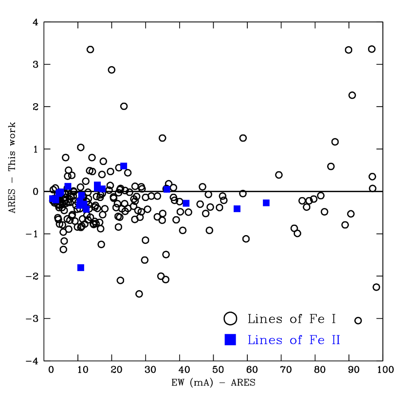
Figure 1: Comparison of EWs measured for a set of Fe I and Fe II lines in HD 140283 using the code by Siqueira-Mello et al. (2014) and EWs measured using ARES.

The complete list of Fe and Ti lines used is shown in Table A, which includes wavelength (Å), excitation potential (eV), log $gf$ values from the VALD and NIST databases, the measured EWs (mÅ), and the derived abundances. Using the errors given for the parameters of the Gaussian profile obtained from the fitting procedure, the uncertainties $\sigma$EW of the equivalent widths were computed based on standard error propagation.

3.2 Calculations

Iron and titanium abundances were derived using equivalent widths, as usual. All other element abundances were derived from fits of synthetic spectra to the observed spectrum of HD 140283. The OSMARCS 1D model atmosphere grid was employed (Gustafsson et al. 2008).

We used the spectrum synthesis code Turbospectrum (Alvarez & Plez 1998), which includes treatment of scattering in the blue and UV domain, molecular dissociative equilibrium, and collisional broadening by H, He, and H₂, following Anstee & O’Mara (1995), Barklem & O’Mara (1997), and Barklem et al. (1998). The calculations used the Turbospectrum molecular line lists (Alvarez & Plez 1998), and atomic line lists from the VALD compilation (Kupka et al. 1999). When available, new experimental oscillator strengths were adopted from literature. In addition, hyperfine structure (HFS) splitting and isotope shifts were implemented when needed and available.

We also performed NLTE calculations for the following ions: C I, O I, Na I, Mg I, Al I, K I, Ca I, Sr II, and Ba II. Atomic models for these species were used in combination with the NLTE MULTI code (Carlsson 1986; Korotin et al. 1999), which facilitates a very good description of the radiation field. The updated version of the MULTI code includes opacities from ATLAS9 (Castelli & Kurucz 2003), which modify the intensity distribution in the UV region.

The lines studied in NLTE are often blended with lines of other species. Proper comparison of the synthesized and observed profiles thus requires a multi-element synthesis. To accomplish this, we fold the NLTE (MULTI) calculations into the LTE synthetic spectrum code SYNTHV (Tsymbal 1996). With these two codes, we calculate synthetic spectra for each region in the vicinity of the line of interest taking (in LTE) all the blending lines located in this region and listed in the VALD database into account. For the lines of interest (treated in NLTE), the corresponding departure coefficients (so-called $b$-factors: $b=n_{\rm i}/n^{*}_{\rm i}$, the ratio of NLTE to LTE atomic level populations) obtained with MULTI code are the input to SYNTHV code, where they are used in the calculation of the line source function, and then for the NLTE line profile. Other possible blending lines are treated in LTE.

3.3 Stellar parameters

Following Paper I, we adopted the stellar parameters $T_{\mathrm{eff}}$ $=5750\pm 100$ K, $\hbox{[Fe/H]}=-2.5\pm 0.2$ and $\xi=1.4\pm 0.1$ km s^-1 from Aoki et al. (2004) and log $g$ $=3.7\pm 0.1$ [g in cgs] from Collet et al. (2009). Using the newly measured EWs, we obtained the iron abundances A(Fe I) $=+4.91\pm 0.07$ and A(Fe II) $=+4.96\pm 0.07$, or $\hbox{[Fe I/H]}=-2.59\pm 0.08$ and $\hbox{[Fe II/H]}=-2.54\pm 0.08$, using the solar abundance A(Fe)${}_{\odot}=+7.50\pm 0.04$ from Asplund et al. (2009). The results are in very good agreement with the literature, as in Gallagher et al. (2010), where [Fe/H]$=-2.59\pm 0.06$ was obtained. For titanium, we found A(Ti I) $=+2.71\pm 0.01$ and A(Ti II) $=+2.69\pm 0.03$, or $\hbox{[Ti I/H]}=-2.24\pm 0.05$ and $\hbox{[Ti II/H]}=-2.26\pm 0.06$, using the solar abundance of titanium A(Ti)${}_{\odot}=+4.95\pm 0.05$ from Asplund et al. (2009). In Table 1 we summarize the atmospheric parameters adopted, together with the iron and titanium abundances.

Figure 2 shows the dependence of [Fe I/H], [Fe II/H], [Ti I/H], and [Ti II/H] on log $(EW/\lambda)$, and on the excitation potential of the lines obtained for HD 140283. The blue solid lines represent the average abundances in each case. The excitation and ionization equilibria of Fe and Ti lines, resulting from the set of atmospheric parameters adopted for HD 140283, confirm the robustness of our choice. However, it should be noted that the surface gravity value may be affected by NLTE effects and by uncertainties in the oscillator strengths of the Fe and Ti lines.

The broadening parameters in HD 140283 were carefully analysed by several authors. We adopted a Gaussian profile to take the effects of macroturbulence, rotational, and instrumental broadening into account.

Table 1: Atmospheric parameters adopted for HD 140283.

	Values
$T_{\mathrm{eff}}$	$5750\pm 100$ K
log $g$	$3.7\pm 0.1$ [g in cgs]
[Fe/H]model	$-2.5\pm 0.2$
$\xi$	$1.4\pm 0.1$ km s-1
[Fe I/H]	$-2.59\pm 0.08$
[Fe II/H]	$-2.54\pm 0.08$
[Ti I/H]	$-2.24\pm 0.05$
[Ti II/H]	$-2.26\pm 0.06$

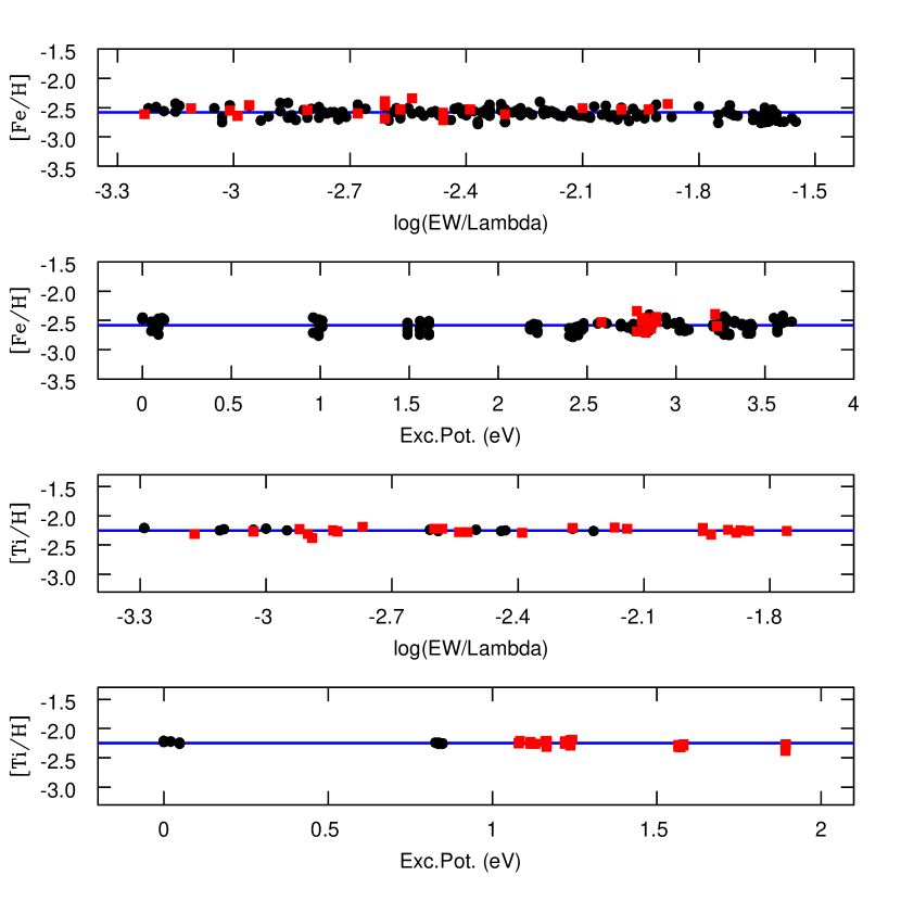
Figure 2: Excitation and ionization equilibria of Fe and Ti lines, resulting from the set of atmospheric parameters for HD 140283. The black dots are the abundances obtained from Ti I and Fe I lines, the red squares are those from Ti II and Fe II lines, and the blue solid lines represent the average abundances.

3.4 Uncertainties in the derived abundances

As described in Paper I, the adopted atmospheric parameters present typical errors of $\Delta$T${}_{\rm eff}=\pm 100$ K, $\Delta$log $g$ $=\pm 0.1$ [g in cgs], and $\Delta\xi=\pm 0.1$ km s^-1. Since the stellar parameters are not independent from each other, the quadratic sum of the various sources of uncertainties is not the best way to estimate the total error budget, otherwise it is mandatory to include the covariance terms in this calculation, and an estimated correlation matrix may introduce uncontrollable error sources.

To compute the total error budget in the abundance analysis arising from the stellar parameters, we created a new atmospheric model with a 100 K lower temperature, determining the corresponding surface gravity and microturbulent velocity with the traditional spectroscopic method. Requiring that the iron abundance derived from Fe I and Fe II lines be identical, we determined the respective log $g$ value, and the microturbulent velocity was found requiring that the abundances derived for individual Fe I lines be independent of the equivalent width values. The result is a model with T${}_{\rm eff}=5650$ K, log $g$ $=3.3$ [g in cgs], and $\xi=1.2$ km s^-1. The abundance analysis was carried out with this new model, and the difference in comparison with the nominal model should represent the uncertainties from the atmospheric parameters.

Observational errors were estimated using the standard deviation of the abundances from the individual lines for each element, and taking into account the uncertainties in defining the continuum, fitting the line profiles, and in the oscillator strengths. For the elements with only one line available, we adopted the observational error from iron as a representative value. The adopted total error budget is the quadratic sum of uncertainties arising from atmospheric parameters and observations.

To estimate the uncertainties in the individual abundances due to the uncertainties in the EWs $\sigma$EW, we recomputed the abundances using $\hbox{EW}+\sigma\hbox{EW}$, and the differences with respect to the nominal values were adopted as the errors. The errors line-by-line are also shown in Table A.

Table 2: Abundance uncertainties due to stellar parameters $\Delta_{par}$, observational errors $\Delta_{obs}$, and adopted total error budget $\Delta_{total}$ for LTE abundances.

Element	$\Delta_{par}$	$\Delta_{obs}$	$\Delta_{total}$
[Fe/H]	$-$0.07	0.07	0.10
[Li/H]	$-$0.08	0.07	0.11
[C/Fe]	$+$0.01	0.07	0.07
[N/Fe]	$-$0.10	0.07	0.12
[O/Fe]	$-$0.15	0.07	0.17
[Na/Fe]	$-$0.04	0.08	0.09
[Mg/Fe]	$-$0.04	0.07	0.08
[Al/Fe]	$-$0.01	0.07	0.07
[Si/Fe]	$-$0.08	0.01	0.08
[K/Fe]	$-$0.06	0.07	0.09
[Ca/Fe]	$-$0.03	0.04	0.05
[Sc/Fe]	$-$0.07	0.06	0.09
[Ti/Fe]	$-$0.07	0.03	0.08
[V/Fe]	$-$0.07	0.08	0.11
[Cr/Fe]	$-$0.08	0.04	0.09
[Mn/Fe]	$-$0.07	0.04	0.08
[Co/Fe]	$-$0.07	0.11	0.13
[Ni/Fe]	$-$0.07	0.05	0.09
[Zn/Fe]	$-$0.07	0.07	0.10
[Sr/Fe]	$-$0.02	0.07	0.07
[Y/Fe]	$-$0.10	0.06	0.12
[Zr/Fe]	$-$0.11	0.05	0.12
[Ba/Fe]	$-$0.09	0.10	0.13
[Ce/Fe]	$-$0.07	0.18	0.19

4 Abundance derivation

Table A shows the line list of elements other than Fe and Ti used in this work, including wavelength (Å), excitation potential (eV), adopted oscillator strength, and abundance derived from each line. The final LTE abundances derived in HD 140283 for all the analysed species are shown in Table 3. The adopted solar abundances from Asplund et al. (2009) are also listed in Table 3. We discuss below each element in terms of lines used, HFS splitting, and abundances adopted. In Table 4 we report the solar isotopic fractions adopted from Asplund et al. (2009) that are relevant for HFS computations, and in Table A we summarize the hyperfine coupling constants adopted for the lines retained in this analysis.

Table 3: LTE abundances. Column 2 gives the solar abundances from Asplund et al. (2009), columns 3, 4, and 5 give the absolute abundance with respect to A(H)=12.0 and the usual logarithmic ratio notation with respect to H and to Fe, respectively.

Ion	A(X)⊙	A(X)	[X/H]	[X/Fe]
Fe I	7.50$\pm$0.04	$+$4.91	$-$2.59	—
Fe II	7.50$\pm$0.04	$+$4.96	$-$2.54	—
Li I	1.05$\pm$0.10	$+$2.14	$+$1.09	—
C(CH)	8.43$\pm$0.05	$+$6.30	$-$2.13	$+$0.46
C I	8.43$\pm$0.05	$+$6.44	$-$1.99	$+$0.60
N(CN)	7.83$\pm$0.05	$+$6.30	$-$1.53	$+$1.06
[O I]	8.69$\pm$0.05	$+$6.95	$-$1.74	$+$0.85
O I	8.69$\pm$0.05	$+$7.11	$-$1.58	$+$1.00
Na I	6.24$\pm$0.04	$+$3.62	$-$2.62	$-$0.04
Mg I	7.60$\pm$0.04	$+$5.27	$-$2.33	$+$0.26
Mg II	7.60$\pm$0.04	$+$5.66	$-$1.95	$+$0.64
Al I	6.45$\pm$0.03	$+$2.96	$-$3.50	$-$0.91
Si I	7.51$\pm$0.03	$+$5.30	$-$2.21	$+$0.38
Si II	7.51$\pm$0.03	$+$5.35	$-$2.16	$+$0.43
K I	5.03$\pm$0.09	$+$2.98	$-$2.05	$+$0.54
Ca I	6.34$\pm$0.04	$+$4.03	$-$2.31	$+$0.27
Ca II	6.34$\pm$0.04	$+$4.43	$-$1.91	$+$0.68
Sc I	3.15$\pm$0.04	$+$0.58	$-$2.58	$+$0.01
Sc II	3.15$\pm$0.04	$+$0.75	$-$2.40	$+$0.18
Ti I	4.95$\pm$0.05	$+$2.71	$-$2.24	$+$0.34
Ti II	4.95$\pm$0.05	$+$2.69	$-$2.26	$+$0.32
V I	3.93$\pm$0.08	$+$1.44	$-$2.49	$+$0.09
V II	3.93$\pm$0.08	$+$1.70	$-$2.23	$+$0.36
Cr I	5.64$\pm$0.04	$+$2.95	$-$2.69	$-$0.11
Cr II	5.64$\pm$0.04	$+$3.32	$-$2.32	$+$0.26
Mn I	5.43$\pm$0.04	$+$2.56	$-$2.87	$-$0.29
Co I	4.99$\pm$0.07	$+$2.69	$-$2.30	$+$0.29
Ni I	6.22$\pm$0.04	$+$3.76	$-$2.46	$+$0.12
Ni II	6.22$\pm$0.04	$+$3.88	$-$2.34	$+$0.25
Zn I	4.56$\pm$0.05	$+$2.22	$-$2.34	$+$0.25
Sr II	2.87$\pm$0.07	$+$0.10	$-$2.77	$-$0.18
Y II	2.21$\pm$0.05	$-$0.78	$-$2.99	$-$0.40
Zr II	2.58$\pm$0.04	$-$0.07	$-$2.65	$-$0.07
Ba II	2.18$\pm$0.09	$-$1.22	$-$3.40	$-$0.81
La II	1.10$\pm$0.04	$<-$1.85	$<-$2.95	$<-$0.36
Ce II	1.58$\pm$0.04	$-$0.83	$-$2.41	$+$0.18
Eu II	0.52$\pm$0.04	$-$2.35	$-$2.87	$-$0.28

In Table 5 we present the complete line list analysed in NLTE, with the respective individual abundances. Below we also give element-by-element information about sources of the NLTE atomic models we used, and we also present the graphical results of the NLTE line synthesis.

Table 4: Isotopic abundance fractions in the solar system from Asplund et al. (2009), relevant for HFS computations adopted in the present work.

Elements	Isotopes	%
Sodium	23Na	100.000
Aluminum	27Al	100.000
Potassium	39K	93.132
	40K	0.147
	41K	6.721
Scandium	45Sc	100.000
Vanadium	50V	0.250
	51V	99.750
Manganese	55Mn	100.000
Zinc	64Zn	48.630
	66Zn	27.900
	67Zn	4.100
	68Zn	18.750
	70Zn	0.620
Barium	130Ba	0.106
	132Ba	0.101
	134Ba	2.417
	135Ba	6.592
	136Ba	7.854
	137Ba	11.232
	138Ba	71.698
Lanthanum	138La	0.091
	139La	99.909
Europium	151Eu	47.81
	153Eu	52.19

Table 5: NLTE abundances derived in HD 140238 using NLTE equivalent width fitting (EW) and NLTE line profile fitting (PF).

Ion	$\lambda$ (Å)	(X/H)+12	[X/H]	Method
C I	8335.14	$+$6.00	$-$2.43	PF
C I	9061.43	$+$5.97	$-$2.46	PF
C I	9062.48	$+$6.03	$-$2.40	PF
O I	7771.94	$+$7.04	$-$1.67	PF
O I	7774.16	$+$6.98	$-$1.73	PF
O I	7775.39	$+$7.00	$-$1.71	PF
O I	8446.36	$+$7.04	$-$1.67	PF
Na I	5889.95	$+$3.37	$-$2.88	PF
Na I	5895.92	$+$3.37	$-$2.88	PF
Na I	8194.82	$+$3.37	$-$2.88	PF
Mg I	4167.27	$+$5.38	$-$2.16	PF
Mg I	4571.10	$+$5.38	$-$2.16	PF
Mg I	4702.99	$+$5.38	$-$2.16	PF
Mg I	5172.68	$+$5.38	$-$2.16	PF
Mg I	5183.60	$+$5.38	$-$2.16	PF
Mg I	5528.40	$+$5.38	$-$2.16	PF
Mg I	5711.09	$+$5.38	$-$2.16	PF
Mg I	8806.76	$+$5.38	$-$2.16	PF
Al I	3944.01	$+$3.70	$-$2.73	PF
Al I	3961.52	$+$3.65	$-$2.78	PF
K I	7698.96	$+$2.78	$-$2.33	PF
Ca I	4226.73	$+$4.04	$-$2.27	PF
Ca I	4283.01	$+$4.21	$-$2.10	EW
Ca I	4289.37	$+$4.14	$-$2.17	EW
Ca I	4302.53	$+$4.15	$-$2.16	EW
Ca I	4318.65	$+$4.09	$-$2.22	EW
Ca I	4425.44	$+$4.18	$-$2.13	EW
Ca I	4434.96	$+$4.07	$-$2.24	EW
Ca I	4435.68	$+$4.17	$-$2.14	EW
Ca I	4454.78	$+$4.04	$-$2.27	EW
Ca I	5188.84	$+$4.20	$-$2.11	EW
Ca I	5261.70	$+$4.15	$-$2.16	EW
Ca I	5265.56	$+$4.20	$-$2.11	EW
Ca I	5349.46	$+$4.22	$-$2.09	EW
Ca I	5512.98	$+$4.09	$-$2.22	EW
Ca I	5581.96	$+$4.22	$-$2.09	EW
Ca I	5588.75	$+$4.11	$-$2.20	EW
Ca I	5590.11	$+$4.22	$-$2.09	EW
Ca I	5594.46	$+$4.19	$-$2.12	EW
Ca I	5857.45	$+$4.17	$-$2.14	EW
Ca I	6102.72	$+$4.14	$-$2.17	EW
Ca I	6122.22	$+$4.14	$-$2.17	EW
Ca I	6162.17	$+$4.05	$-$2.26	EW
Ca I	6169.56	$+$4.17	$-$2.14	EW
Ca I	6439.07	$+$4.08	$-$2.23	EW
Ca I	6462.56	$+$4.06	$-$2.25	EW
Ca I	6471.66	$+$4.08	$-$2.23	EW
Ca I	6493.78	$+$4.10	$-$2.21	EW
Ca I	6499.65	$+$4.23	$-$2.08	EW
Ca I	7148.15	$+$4.19	$-$2.12	EW
Ca I	7326.14	$+$4.19	$-$2.12	EW
Ca II	3933.68	$+$4.15	$-$2.16	PF
Ca II	3968.47	$+$4.15	$-$2.16	PF
Ca II	8498.02	$+$4.15	$-$2.16	PF
Ca II	8542.09	$+$4.15	$-$2.16	PF
Ca II	8662.14	$+$4.15	$-$2.16	PF
Sr II	4077.72	$+$0.02	$-$2.90	PF
Sr II	4215.52	$+$0.07	$-$2.85	PF
Sr II	10327.31	$+$0.00	$-$2.92	PF
Ba II	4554.03	$-$1.07	$-$3.24	PF
Ba II	6141.70	$-$1.07	$-$3.24	PF
Ba II	6496.92	$-$1.01	$-$3.18	PF

4.1 Light elements

$Lithium$. We derived the LTE Li abundance A(Li) $=+2.14$ based on the Li I lines located at 6103 Å and 6707 Å (see Fig. 3). The wavelength and oscillator strength values were adopted from NIST, based on calculations by Yan & Drake (1995). NLTE corrections are given in Asplund et al. (2006) for the two Li lines in HD 140283: $+0.09$ dex for 6103 Å and $+0.03$ for 6707 Å. The corrected Li abundance A(Li) $=+2.20$ is in excellent agreement with the NLTE abundance from Asplund et al. (2006).

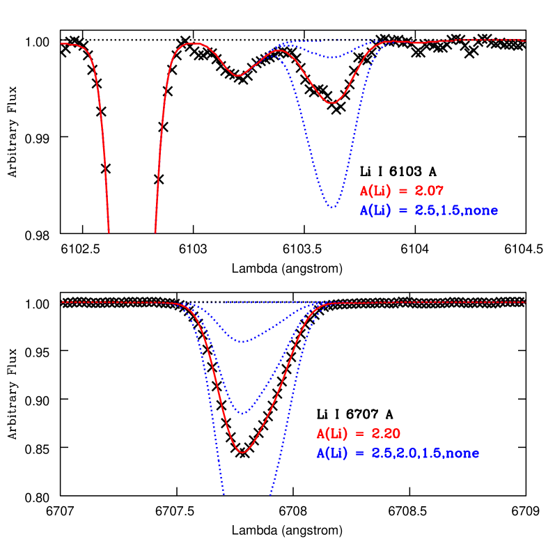
Figure 3: LTE lithium abundance in HD 140283 from the Li I lines located at 6103 Å (upper panel) and 6707 Å (lower panel). Observations (crosses) are compared with synthetic spectra computed with different abundances (blue dotted lines), as well as with the adopted abundances (red solid lines).

$Carbon$. In Paper I we analysed the CH A-X electronic transition band (G band) in HD 140283, showing a very good agreement between the observed spectrum and the computation using the LTE carbon abundance A(C) $=+6.30$ adopted from Honda et al. (2004a). In fact, several CH lines were analysed and all of them presented a good fit, leading us to assume that they are properly taken into account.

It was also possible to use three C I lines: 8335.14 Å, 9061.43 Å, and 9062.48 Å. They are free of telluric and other atomic or molecular lines. The lines of C I in the visual part of the spectrum are not detectable. The LTE carbon abundance derived from these atomic transitions A(C) $=+6.44$ is slightly higher in comparison with the result from molecular bands.

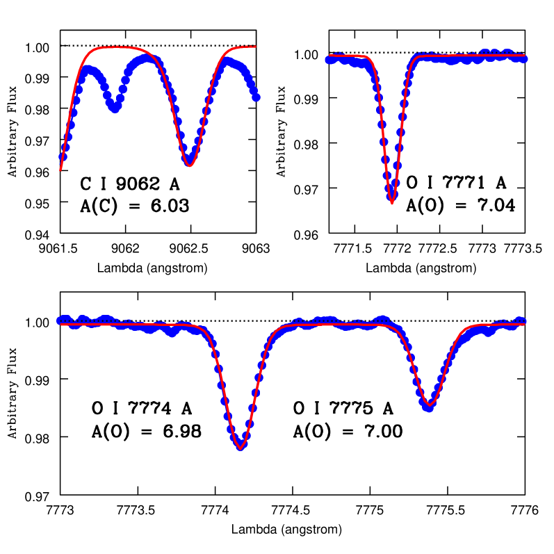
Figure 12: NLTE carbon abundance in HD 140283 from C I 9062.48 Å line (upper left panel) and NLTE oxygen abundance from the red O I triplet: 7771.94 Å (upper right panel), 7774.16 Å, and 7775.39 Å (lower panel) lines. Observations (blue circles) are compared with synthetic spectra computed with the adopted abundances (red solid lines).

The same C I lines were analysed in NLTE (see upper left panel in Fig. 12 for the 9062.48 Å line). To perform this work, we used the carbon atomic model first proposed by Lyubimkov et al. (2015). Our calculations show that NLTE effects are very strong in the analysed lines, and act towards a strengthening of their equivalent widths: the ratio between NLTE and LTE EWs reaches a factor around 3. This means that simply analysing the program carbon lines in LTE approximation results in the derived abundance overestimate by about $0.4-0.5$ dex (as it should be for the generally weak lines where equivalent width linearly depend upon the number of absorbing atoms). The same conclusion was given by Asplund (2005), who noted that strong NLTE effects in high-excitation neutral carbon lines are due to the decrease of source function (compared to the Planck function). In particular this is valid for near-infrared C I lines. Fabbian et al. (2006) also predict strong NLTE corrections in the carbon abundances in extremely metal-poor stars of $\sim$$0.4$ dex, in good agreement with the present result.

We find a difference between the C abundance deduced from CH and that from C I lines computed in LTE and NLTE of $\Delta($C(CH) $-$ C(C I)${}_{LTE})$ $=-0.14$ dex, and $\Delta($C(CH) $-$ C(C I)${}_{NLTE})$ $=+0.30$ dex, respectively. The CH lines forming in the upper atmosphere might be affected in a 3D modelling calculation (Asplund 2005).

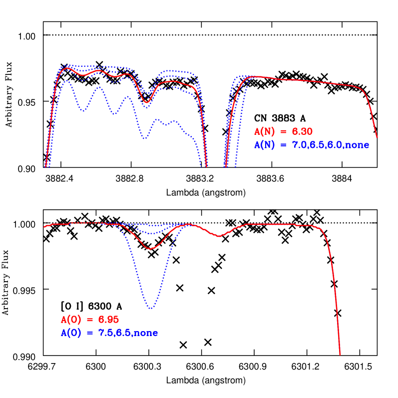
Figure 11: LTE nitrogen abundance in HD 140283 from CN(0,0) bandhead at 3883 Å (upper panel) and LTE oxygen abundance from [O I] 6300.31 Å line (lower panel). Symbols are the same as in Fig. 3.

$Nitrogen$. The bandhead of CN(0,0) B₂$\Sigma$ $-$ X₂$\Sigma$ at 3883 Å gives A(N) $=+6.30$, assuming the abundances A(C) $=+6.30$ and A(O) $=+7.00$. In Fig. 11 (upper panel) we present the synthetic spectra fitting to the CN bandhead. This profile is located in the blue wing of the H8 line of the Balmer series, taken into account in the calculations.

$Oxygen$. The forbidden [O I] 6300.31 Å line is free from NLTE effects (Kiselman 2001), and therefore it is the best oxygen abundance indicator. The line was inspected for telluric lines in each of the original exposures. From our series of observations, four of the spectra observed in July had to be discarded, given that the telluric lines were masking the oxygen line. We then proceeded to co-add the other 19 spectra, and were able to obtain a weak, but measurable line (see lower panel in Fig. 11). We derive an abundance of A(O) $=+6.95$, considered in this calculation A(C) $=+6.30$ (C derived from CH lines) and A(N)$=+6.30$.

The triplets at 7771-7775 Å and 8446 Å were also checked to compute the LTE O abundance A(O) $=+7.11$ in HD 140283. Adopting an average of different models presented in Behara et al. (2010) for the NLTE corrections to be applied on the triplet 7771-7775 Å lines ($-0.13$ dex, $-0.10$ dex, and $-0.10$ dex, respectively), we obtain A(O) $=+6.97$ from this triplet, in excellent agreement with the result derived using the forbidden line.

The triplets at 7771-7775 Å (see Fig. 12) and 8446 Å were also analysed in NLTE. Our NLTE model of this atom was first described in Mishenina et al. (2000), and then updated by Korotin et al. (2014). An updated model was applied to study the NLTE abundance of this element in cepheids, and its distribution in the Galactic disc (see, for instance, Korotin et al. 2014; Martin et al. 2015). We obtain a NLTE oxygen abundance A(O) $=+7.02$ (or [O/Fe] $=+0.90$), in agreement with the derived LTE abundances corrected for NLTE effects.

4.2 $\alpha$-elements: Mg, Si, S, and Ca

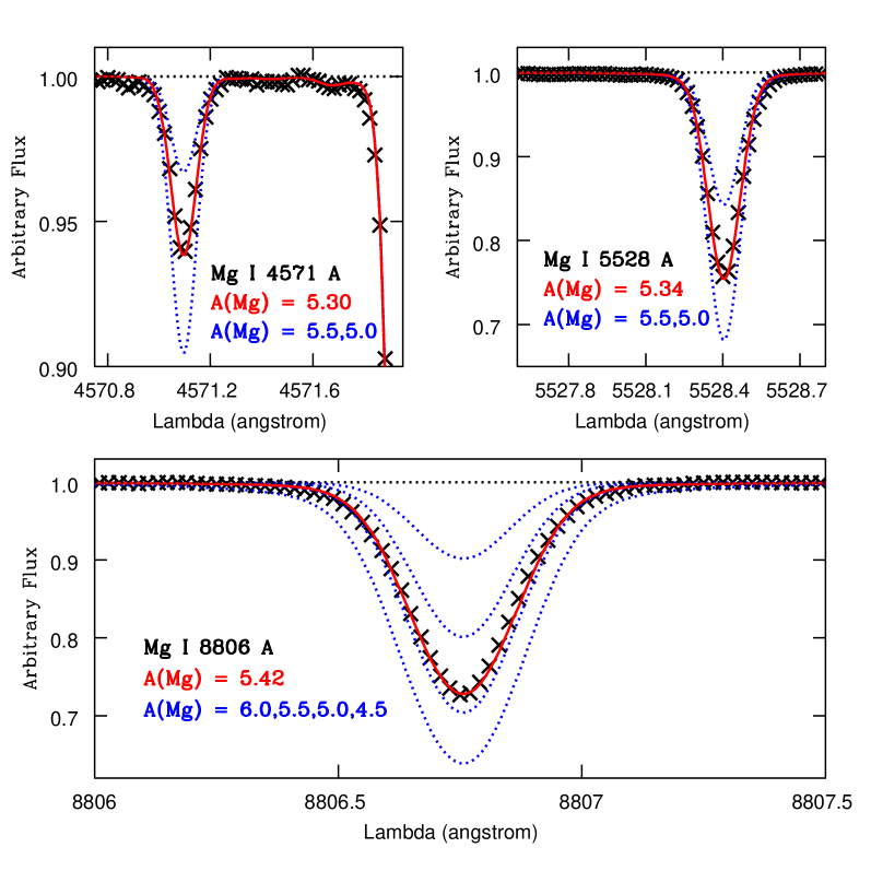
Figure 13: LTE magnesium abundance in HD 140283 from Mg I 4571.10 Å (upper left panel), Mg I 5528.40 Å (upper right panel), and Mg I 8806.76 Å (lower panel) lines. Symbols are the same as in Fig. 3.

$Magnesium$. After checking the Mg I lines used by Zhao et al. (1998) in the solar spectrum and the bluer lines used by Cayrel et al. (2004) for metal-poor stars, we retained 12 lines from an initial list of 21 profiles to derive the LTE abundance A(Mg I) $=+5.27$. The oscillator strengths were adopted from the critical compilation presented in Kelleher & Podobedova (2008a). The individual abundances are consistent among the lines (see upper panels in Fig. 13), with the exception of Mg I 8806.76 Å, which is $0.13$ dex higher than the average abundance (see lower panel in Fig. 13).

In addition, it was possible to use two Mg II lines with the spectrum of HD 140283: 4481.13 Å and 4481.15 Å. The derived LTE abundance A(Mg II) $=+5.66$ is higher than the value obtained from the neutral species, but both Mg II lines are blended and the result should be used with caution.

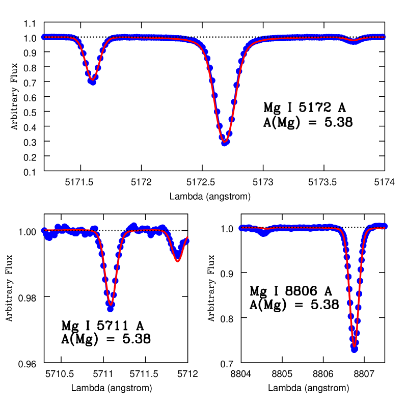
Figure 14: NLTE magnesium abundance in HD 140283 from Mg I 5172.68 Å (upper panel), Mg I 5711.09 Å (lower left panel), and Mg I 8806.76 Å (lower right panel) lines. Symbols are the same as in Fig. 12.

Seven magnesium lines were selected for NLTE abundance determination. All these lines have very well-defined profiles, which provide a robust NLTE abundance of this element (see Fig. 14). To generate Mg I line profiles, we used the NLTE Mg I atomic model described in detail by Mishenina et al. (2004). This model was used in several studies, in particular, in the determination of the magnesium abundance in a sample of metal-poor stars (Andrievsky et al. 2010).

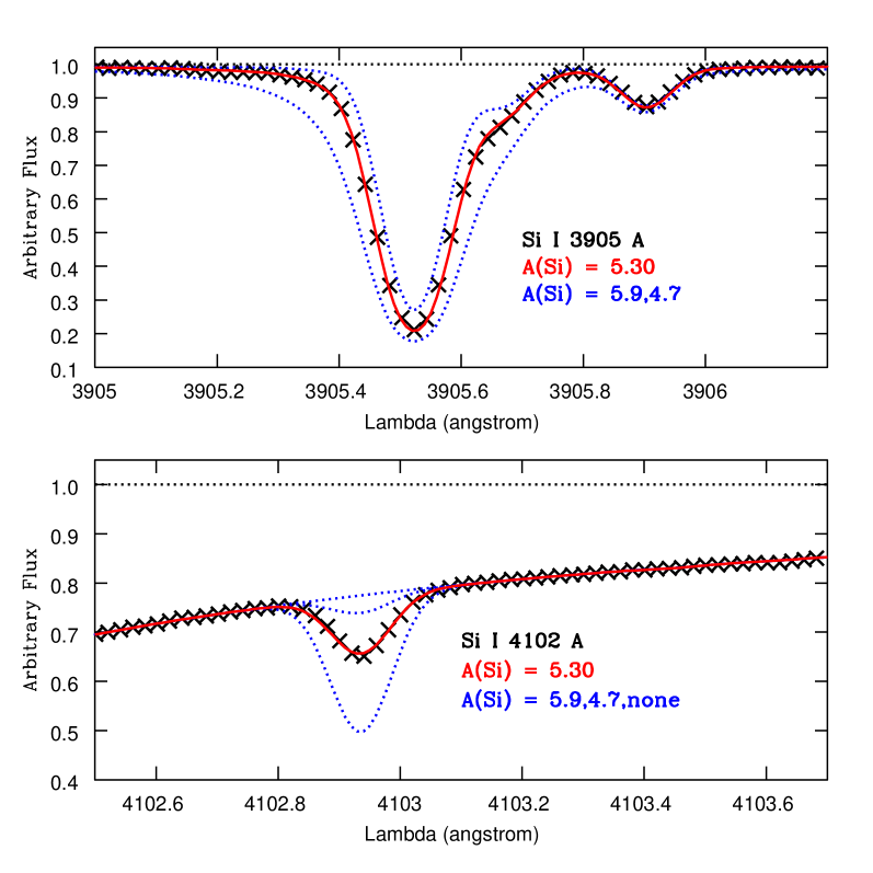
Figure 15: LTE silicon abundance in HD 140283 from Si I 3905.52 Å (upper panel) and Si I 4102.936 Å (lower panel) lines. Symbols are the same as in Fig. 3.

$Silicon$. The main Si abundance indicators are the Si I lines at 3905.52 Å and 4102.94 Å. The line at 3905 Å is blended with CH lines, but these molecular lines are weak enough in a rather hot subgiant such that the Si I line can be used. On the other hand, the line at 4102 Å is located in the red wing of the H$\delta$ line, and therefore it was necessary to take the hydrogen line in the spectrum synthesis into account. Fig. 15 shows the LTE synthetic spectra used for these lines in HD 140283. It was possible to use another three weaker Si I lines located at 5645.61 Å, 5684.48 Å, and 7034.90 Å, with individual abundances in good agreement with the previous transitions. The final LTE Si abundance obtained was A(Si I)$=+5.30$. Because of the good quality of our data, it was possible to derive the LTE silicon abundance from the ionized species A(Si II)$=+5.35$, using the Si II 6371.37 Å line.

$Sulfur$. Three S I lines, which are potentially available for the abundance determination in metal-poor stars, are located at 9212.86 Å, 9228.09 Å, and 9237.54 Å. Unfortunately, the first line is severely blended with telluric lines, and the other two lines are on a small gap in the spectrum. As a consequence, a reliable sulfur abundance is not presented here for HD 140283.

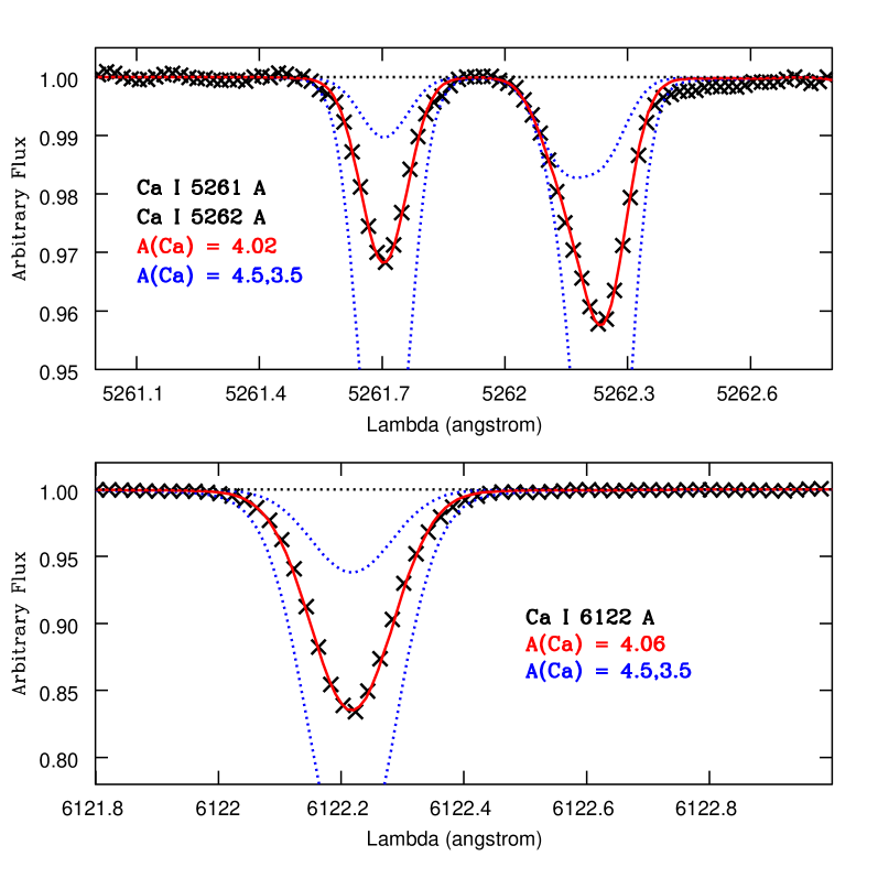
Figure 16: LTE calcium abundance in HD 140283 from Ca I 5261.70 Å, Ca I 5262.24 Å (upper panel), and Ca I 6122.23 Å (lower panel) lines. Symbols are the same as in Fig. 3.

$Calcium$. To derive the LTE Ca abundance, 36 Ca I lines were used to obtain A(Ca I)$=+4.03$. We adopted the log $gf$ values from Spite et al. (2012). Because of the high-quality spectrum, even weak and blended lines are useful, as shown in Fig. 16.

We inspected a few Ca II lines to evaluate the LTE calcium abundance from the ionized species. The presence of a strong NLTE effect, however, does not permit us to use most of these transitions. The LTE abundance A(Ca II)$=+4.43$ was derived based only on the Ca II 8927.36 Å line. We obtained a difference of $+0.40$ dex in comparison with the abundance derived from transitions of the neutral element. Mashonkina et al. (2007) analysed HD 140283 in their study of neutral and singly-ionized calcium in late-type stars, and the LTE results show a difference of $+0.30$ dex. Their NLTE abundances are [Ca I/Fe] $=+0.29\pm 0.06$ and [Ca II/Fe] $=+0.24$. Using similar atmospheric parameters for this star, Spite et al. (2012) found the NLTE abundances A(Ca I) $=+4.12\pm 0.04$ and A(Ca II) $=+4.08\pm 0.05$. Our LTE abundance shows that the departure from LTE is not strong for neutral calcium in this star.

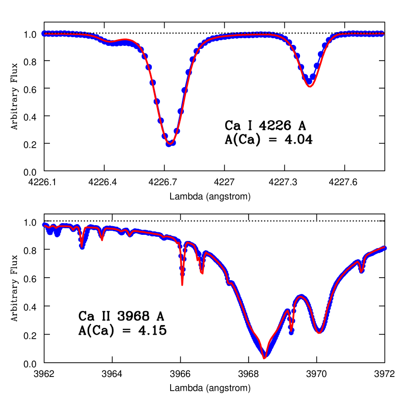
Figure 17: NLTE calcium abundance in HD 140283 from Ca I 4226.73 Å (upper panel) and Ca II 3968.47 Å (lower panel) lines. Symbols are the same as in Fig. 12.

The NLTE abundance A(Ca) $=+4.14$ was determined from the average of 35 lines, including: i) the EW analysis of 30 Ca I lines with 10 $<$ EW(mÅ) $<$ 40; ii) the profile of five other lines, namely the strongest line of this atom at 4226.73 Å (see upper panel in Fig. 17); the H and K Ca II lines (see lower panel in Fig. 17); and another three Ca II lines located in the red. The NLTE atomic model was described in Spite et al. (2012), where it was used for the study of halo metal-poor stars.

4.3 Odd-Z elements: Na, Al, and K

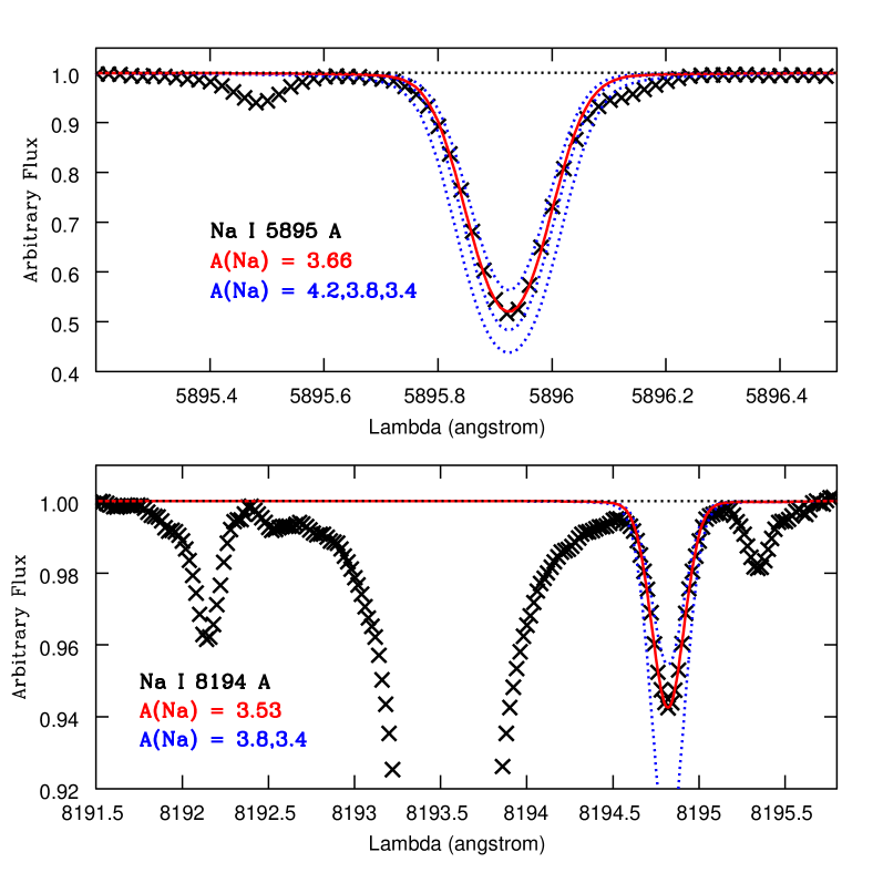
Figure 18: LTE sodium abundance in HD 140283 from Na I 5895.92 Å (upper panel) and Na I 8194.82 Å (lower panel) lines. Symbols are the same as in Fig. 3.

$Sodium$. To derive the LTE sodium abundance we used an initial line list based on Baumüller et al. (1998) with updated oscillator strengths from Kelleher & Podobedova (2008a). After checking 13 Na I lines, the final result A(Na I) $=+3.62$ is based on five sodium lines. ²³Na is the only stable isotope representing the sodium abundance, with nuclear spin I $=3/2$ and therefore exhibiting HFS. The hyperfine coupling constants are adopted from Das & Natarajan (2008) and Safronova et al. (1999). When not available, these constants were assumed to be null. The HFS for each line were computed by employing a code described and made available by McWilliam et al. (2013). Fig. 18 shows in the upper panel the adopted synthetic spectrum for Na I 5895.92  Å and Na I 8194.82 Å lines as example of typical fitting procedures.

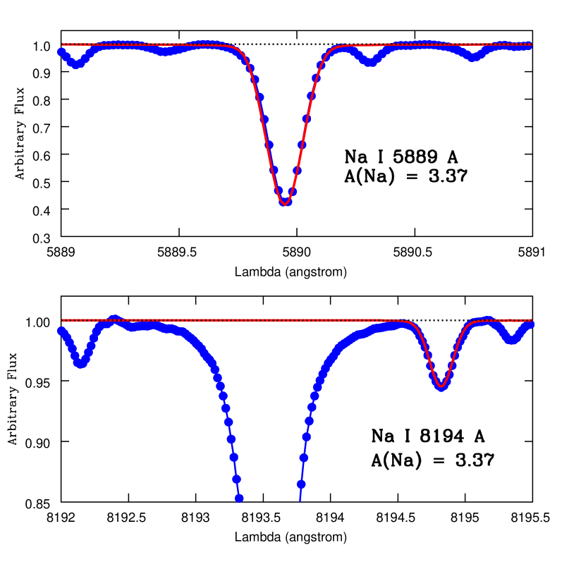
Figure 19: NLTE sodium abundance in HD 140283 from Na I 5889.95  Å (D₂) (upper panel) and Na I 8194.82 Å (lower panel) lines. Symbols are the same as in Fig. 12.

A NLTE atomic model of this element was presented for the first time in Korotin & Mishenina (1999) and then updated by Dobrovolskas et al. (2014). We analysed three Na I lines: D₁, D₂, and the line at 8194.82 Å. Synthesized NLTE profiles fitted to the observed sodium line profiles are shown in Fig. 19, and the final NLTE abundance A(Na I) $=+3.37$ was adopted.

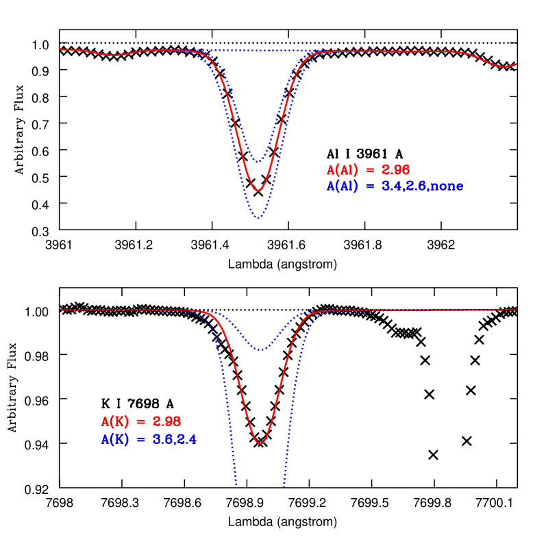
Figure 20: LTE aluminum abundance in HD 140283 from Al I 3961.52  Å line (upper panel) and potassium abundance from K I 7698.96  Å line (lower panel). Symbols are the same as in Fig. 3.

$Aluminum$. The only stable isotope for aluminum is ²⁷Al and to derive the Al abundance we used the resonance doublet Al I 3944.01 Å and Al I 3961.52 Å, taking the CH line blending with the first line into account. The local continuum around the Al I 3961.52 Å line is defined by the blue wings of the H$\varepsilon$ and H Ca II lines, which were taken into account in the spectrum synthesis. ²⁷Al has nuclear spin I $=5/2$ and we adopted the hyperfine coupling constants from Nakai et al. (2007) and Brown & Evenson (1999), with updated oscillator strengths from Kelleher & Podobedova (2008b). Fig. 20 shows in the upper panel the LTE synthetic spectra used for Al I 3961.52 Å as an example. The adopted LTE abundance is A(Al I)$=+2.96$ and must be corrected for NLTE effects.

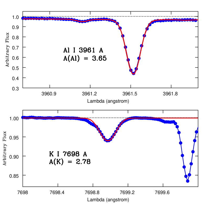
Figure 21: NLTE aluminum abundance in HD 140283 from Al I 3961.52 Å (upper panel) and NLTE potassium abundance from the K I 7698.96 Å line (lower panel) lines. Symbols are the same as in Fig. 12.

The NLTE Al I atomic model presented in Andrievsky et al. (2008) was employed and the result of the profile fitting for Al I 3961.52 Å line is shown in Fig. 21 (upper panel). The final NLTE abundance A(Al I)$=+3.68$ is $0.72$ dex higher than the LTE result.

As it was stated above, in some cases the NLTE profile synthesis should be combined with the LTE synthesis, which takes the blending lines in the vicinity of the studied line into account. For instance, we would get the wrong result if we derived the NLTE abundance from UV Al I lines only using the pure MULTI NLTE profiles, since these lines are located in the wings of very strong H and K Ca II lines. Therefore it is absolutely necessary to take continuum distortion in their vicinity into account. This is made through a combination of calculations with the codes MULTI NLTE and SYNTHV LTE, which provides a correct aluminum abundance.

$Potassium$. The final LTE potassium abundance A(K I) $=+2.98$ was only derived from the K I 7698.96 Å line, as shown in the lower panel of Fig. 20. The other red doublet component at 7665 Å is strongly blended with telluric lines and was excluded. For this element, we adopted the isotopic abundance fractions in the solar system, as described in Asplund et al. (2009) and reproduced in Table 4. The HFS was computed taking into account the major potassium isotope ³⁹K, which has nuclear spin I $=3/2$. We adopted hyperfine coupling constants from Belin et al. (1975) and Falke et al. (2006), with updated oscillator strength from Sansonetti (2008).

A NLTE K I atomic model was presented in Andrievsky et al. (2010), where it was first employed to derive potassium NLTE abundances in a sample of extremely metal-poor halo stars. This model was used to synthesize the profile of the K I 7698.96 Å line in HD 140283 (see lower panel in Fig. 21), which gives A(K I) $=+2.78$ as the final abundance.

4.4 Iron-peak elements: Sc, Ti, V, Cr, Mn, Fe, Co, Ni, and Zn

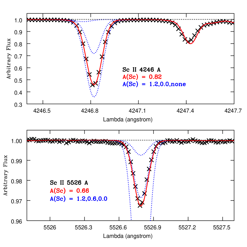
Figure 22: LTE scandium abundances in HD 140283 from Sc II 4246.82  Å (upper panel) and Sc II 5526.79 Å (lower panel) lines. Symbols are the same as in Fig. 3.

$Scandium$. We were able to use two Sc I lines to derive the scandium abundance. The lines located at 4020.39 Å and 4023.68 Å present low excitation potential and the average abundance A(Sc I)$=+0.58$ should suffer from over-ionization via NLTE effects (Zhang et al. 2008). ⁴⁵Sc is the only stable scandium isotope, with nuclear spin I $=7/2$, and to compute the HFS we adopted hyperfine coupling constants from Childs (1971), Siefart (1977), and Başar et al. (2004). On other hand, the ionized species presented 19 useful lines, covering a wider range in wavelengths and excitation potential values. The average result A(Sc II) $=+0.75$ is higher in comparison with the abundance from the neutral species and it is not affected strongly by NLTE effects, at least at solar metallicity (see Asplund et al. 2009). The hyperfine coupling constants were adopted from Villemoes et al. (1992), Mansour et al. (1989), and Scott et al. (2015). In Fig. 22 we show the fitting procedures used for the Sc II 4246.82 Å and Sc II 5526.79 Å lines as examples.

$Titanium$. For titanium, we applied equivalent widths to derive the final abundances A(Ti I) $=+2.71$ and A(Ti II) $=+2.69$ (Sect. 3.1).

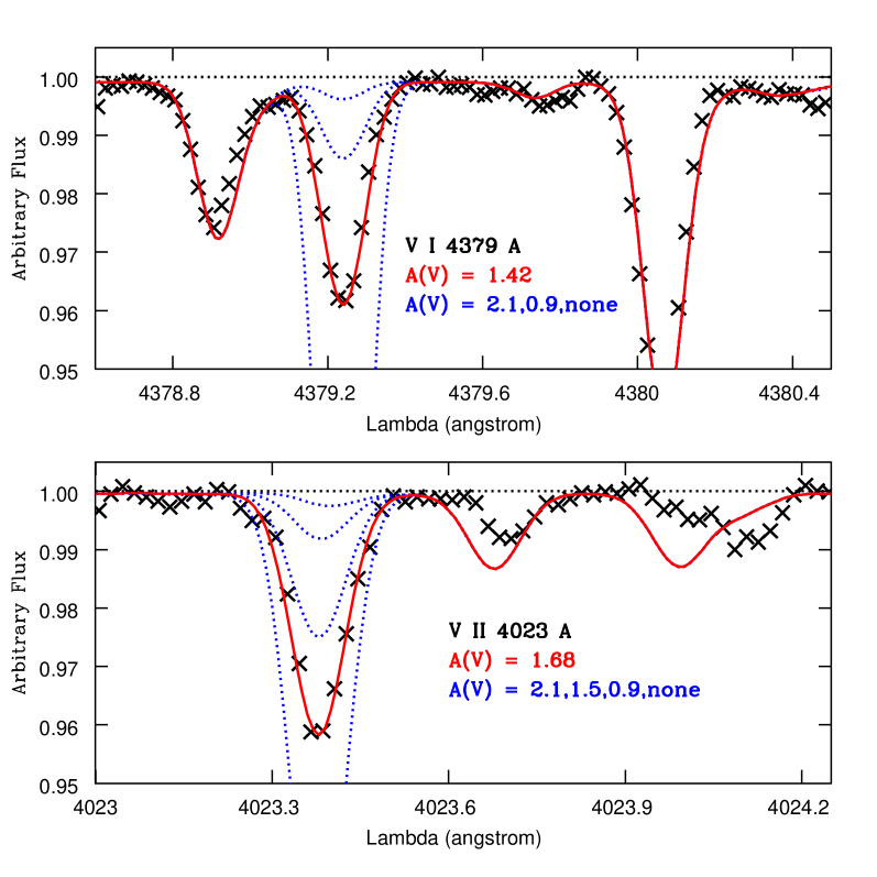
Figure 23: LTE vanadium abundances in HD 140283 from V I 4379 Å (upper panel) and V II 4023 Å (lower panel) lines. Symbols are the same as in Fig. 3.

$Vanadium$. In Paper I we analysed five V I lines and seven V II lines to derive the vanadium abundances A(V I) $=+1.35\pm 0.10$ and A(V II) $=+1.72\pm 0.10$, respectively. The average result A(V) $=+1.56\pm 0.11$ is in good agreement with A(V) $=1.55$ from Honda et al. (2004a), derived in their analysis from three lines (see Table 3 in Siqueira-Mello et al. 2012 for details). We adopted seven V I and eight V II lines, including HFS based on hyperfine coupling constants from Unkel et al. (1989), Palmeri et al. (1995), Armstrong et al. (2011), Gyzelcimen et al. (2014), and Wood et al. (2014), with nuclear spin I $=7/2$. We only used the major V isotope in the computations (see Table 4). The oscillator strengths were adopted from Whaling et al. (1985) for V I and from Wood et al. (2014) for V II. We obtained A(V I) $=+1.44$ and A(V II) $=+1.70$, in agreement with the previous results. In addition, the final abundances derived from V I and V II lines are more consistent in the present analysis. In Fig. 23 we show the V I 4379.230 Å line (upper panel) and the V II 4023.378  Å line (lower panel) as examples. The differences measured between the two ionization stages should be explained by strong NLTE effects expected for V I lines.

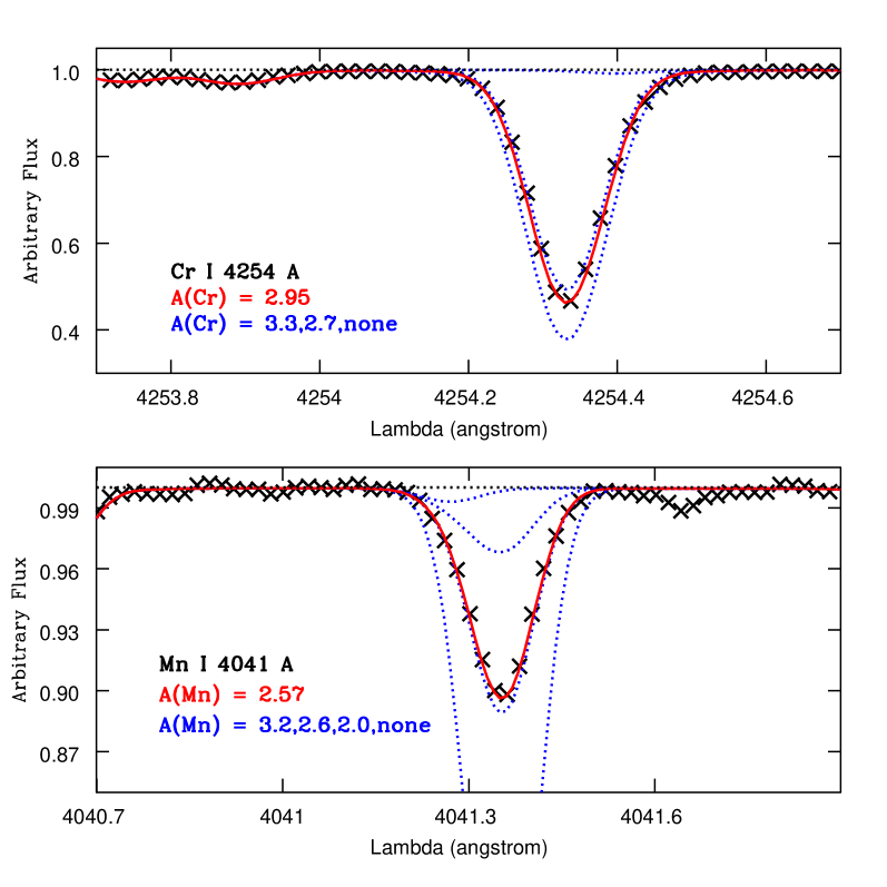
Figure 24: LTE chromium abundance in HD 140283 from Cr I 4254.33 Å line (upper panel) and manganese abundance from Mn I 4041.35 Å line (lower panel). Symbols are the same as in Fig. 3.

$Chromium$. We derived individual chromium abundances for 28 Cr I lines, but we excluded the transitions located at 4756.11 Å and 5237.35 Å because of the higher abundances in comparison with results from other lines, and we obtained the abundance A(Cr I) $=+2.95$ based on seven Cr I lines. The fitting procedure used for Cr I 4254.33 Å line is shown in Fig. 24. In addition, it was possible to use seven Cr II lines in HD 140283 to derive the abundance A(Cr II) $=+3.32$, higher by 0.37 dex than the result obtained from the neutral species.

$Manganese$. The only manganese stable isotope is ⁵⁵Mn, with nuclear spin I $=5/2$. In addition to the three lines belonging to the resonance triplet (Mn I 4030.75 Å, 4033.06 Å, and 4034.48 Å), it was also possible to measure 13 subordinate lines. We took the HFS properly into account based on the hyperfine structure line component patterns from Den Hartog et al. (2011), which also present the sources for hyperfine coupling constants. It is well known that the abundances derived from the triplet resonance lines are systematically lower in comparison with the results from subordinate lines in very metal-poor giant stars. Indeed, the result we obtained for HD 140283 using the triplet A(Mn I) $=+2.31$ is lower than A(Mn I) $=+2.56$ derived from the subordinate lines. The resonance triplet lines are more susceptible to NLTE effects, and for this reason we did not include them in the average Mn abundance. The line Mn I 4041.35 Å is shown in Fig. 24 (lower panel).

$Iron$. We used equivalent widths to derive the final abundances A(Fe I) $=+4.91$ and A(Fe II) $=+4.96$, as described in Sect. 3.1.

$Cobalt$. Individual cobalt abundances were derived from 17 Co I lines. The final abundance A(Co I) $=+2.69$ was computed excluding the lines located at 3861.16 Å and 3873.11 Å because of the higher differences in comparison with the average abundance.

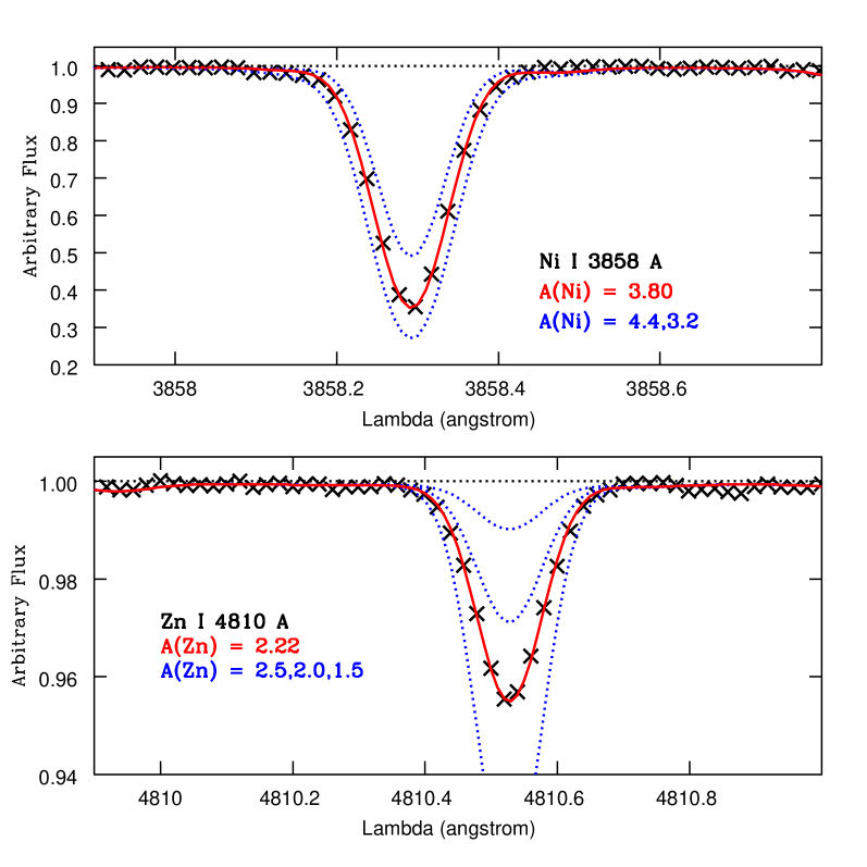
Figure 25: LTE nickel abundance in HD 140283 from Ni I 3858.29 Å line (upper panel) and zinc abundance from Zn I 4810.53 Å line (lower panel). Symbols are the same as in Fig. 3.

$Nickel$. For this element we derived the abundance A(Ni I) $=+3.76$ based on 43 Ni I lines. In Fig. 25 (upper panel) we show the Ni I 3858.29 Å line. We were also able to use the Ni II 3769.46 Å line in the present spectrum to derive the abundance A(Ni II) $=+3.88$ in this star.

$Zinc$. The isotopic structure of zinc is complex (see Table 4), but HFS is not needed to be accounted for, therefore, we assumed Zn as having a unique isotope with wavelengths dominated by the ⁶⁴Zn. The abundance A(Zn I) $=+2.21$ was derived from the Zn I  4722.15 Å and Zn I 4810.53 Å (see Fig. 25, lower panel) lines, with oscillator strengths adopted from Roederer & Lawler (2012).

4.5 Neutron-capture elements

$Strontium$. In HD 140283 the Sr abundance was derived based on three Sr II lines located at 4077.72 Å, 4215.52 Å, and 10327.31 Å. These transitions show HFS effects, but hyperfine coupling constants only exist for ⁸⁷Sr (Borghs et al. 1983), which accounts for less than 7% of Sr (Asplund et al. 2009). In addition, the atomic lines from the even isotopes ⁸⁴Sr, ⁸⁶Sr, and ⁸⁸Sr appear as single lines due to the small isotopic splitting for Sr (Hauge 1972). In conclusion, we treated each Sr line as a single component, with oscillator strengths adopted from Gratton & Sneden (1994), which gives an average abundance of A(Sr II) $=+0.10$. In the upper panel of Fig. 4, we show the fitting procedure used for the Sr II 4077.72 Å line.

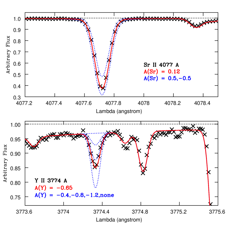
Figure 4: LTE strontium abundance in HD 140283 from Sr II 4077.72 Å line (upper panel) and yttrium abundance from Y II 3774.33 Å line (lower panel). Symbols are the same as in Fig. 3.

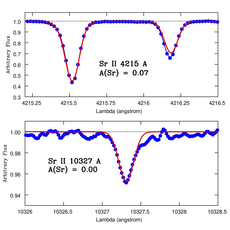
Figure 26: NLTE strontium abundance in HD 140283 from Sr II 4215.52 Å (upper panel) and Sr II 10327.31 Å (lower panel) lines. Symbols are the same as in Fig. 12.

Our NLTE strontium atomic model was described in Andrievsky et al. (2011), where it was applied to a sample of metal-poor stars. We analysed the same two blue Sr II lines at 4077.72 Å and 4215.52 Å (see upper panel in Fig. 26), and a third line in the near-infrared located at 10327.31 Å (see lower panel in Fig. 26), with a final NLTE abundance A(Sr II) $=+0.03$ as the adopted result.

In Andrievsky et al. (2011) the NLTE corrections were calculated for the Sr II 4077.72 Å, 4215.52 Å, besides near-infrared lines for different temperatures and gravities. Considering Fig. 7 of Andrievsky et al. (2011), at $T_{\mathrm{eff}}$ $=5750$ K and log $g$ $=3.7$ the correction should be small and positive. We obtained a NLTE strontium abundance that is slightly lower than the LTE abundance. We suggest that main reasons for this discrepancy can be the result of: a) the LTE results from Turbospectrum may use slightly different atomic constants; and b) this star is more metal-rich ([Fe/H] $=-2.59$) than the calculations for [Fe/H] $=-3.0$ given in Andrievsky et al. (2011).

$Yttrium$. For yttrium it was possible to check in LTE five Y II lines, using oscillator strengths adopted from Hannaford et al. (1982) and Grevesse et al. (2015), with A(Y II) $=-0.78$ as the final abundance. The synthetic profile adopted for Y II 3774.33 Å is shown in Fig. 4 (lower panel), which takes the continuum affected by the H11 line from the Balmer series into account.

$Zirconium$. After inspecting the spectrum, we decided to retain only the three best Zr II lines available, located at 3836.76 Å, 4208.98 Å and 4443.01 Å, to derive the LTE zirconium abundance. The log $gf$ values were adopted from Biémont et al. (1981), with final LTE abundance of A(Zr II) $=-0.07$ (see Fig. 5).

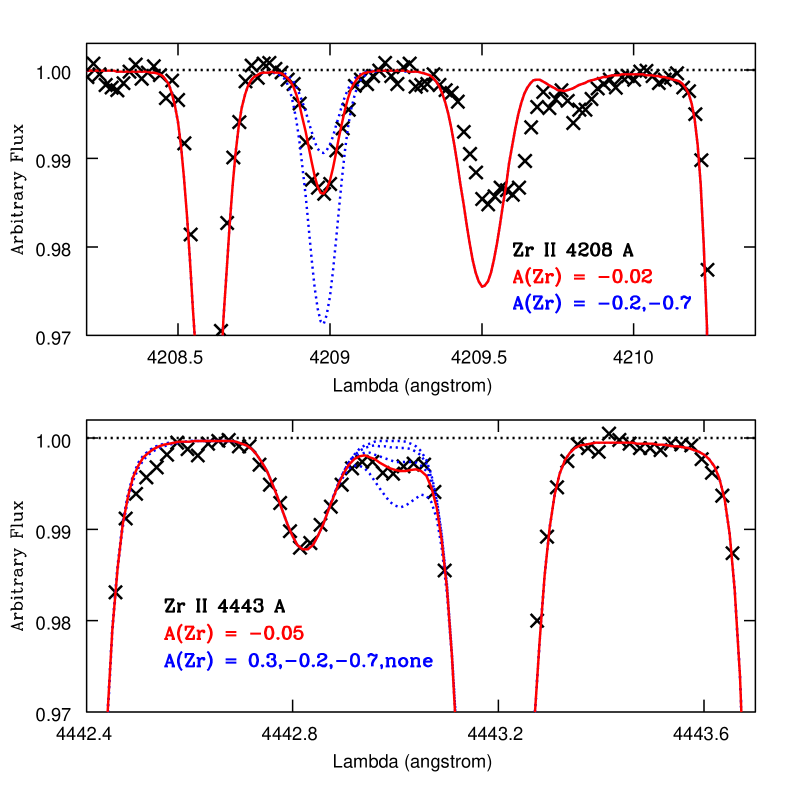
Figure 5: LTE zirconium abundance in HD 140283 from Zr II 4208.98 Å (upper panel) and Zr II 4443.01 Å (lower panel) lines. Symbols are the same as in Fig. 3.

$Barium$. The LTE barium abundance was previously analysed in Paper I, based on the Ba II 4554.03 and Ba II 4934.08 Å lines, with oscillator strengths adopted from Gallagher (1967) and hyperfine structure line component patterns from McWilliam (1998). We added two other Ba II lines, located at 6141.71 Å and 6496.90 Å, with oscillator strengths and HFS from Barbuy et al. (2014). With nuclear spin I $=3/2$, we took the Ba isotopic nuclides into account according to Table 4.

Figure 6 shows the synthetic profiles computed for the Ba II lines. The blue wing of the Ba II 4934.08 Å line is blended with Fe I 4934.01 Å, which we took properly into account using log $gf$ $=-0.59$, adjusted to describe the observed spectrum. The individual abundance agrees with the result derived from the clear Ba II 4554.03Å line. To compute the profile for Ba II 6141.71 Å, it is important to include a blend with Fe I 6141.73 Å for which we adopted log $gf$ $=-1.60$ (Barbuy et al. 2014). For Ba II 6496.90  Å there is a telluric line located in the blue wing in the present spectrum. The individual abundance agrees with that derived from 6141.71 Å line, but it is slightly higher in comparison with the results from the first two Ba lines. We decided to adopt A(Ba II) $=-1.22$ as the final LTE abundance.

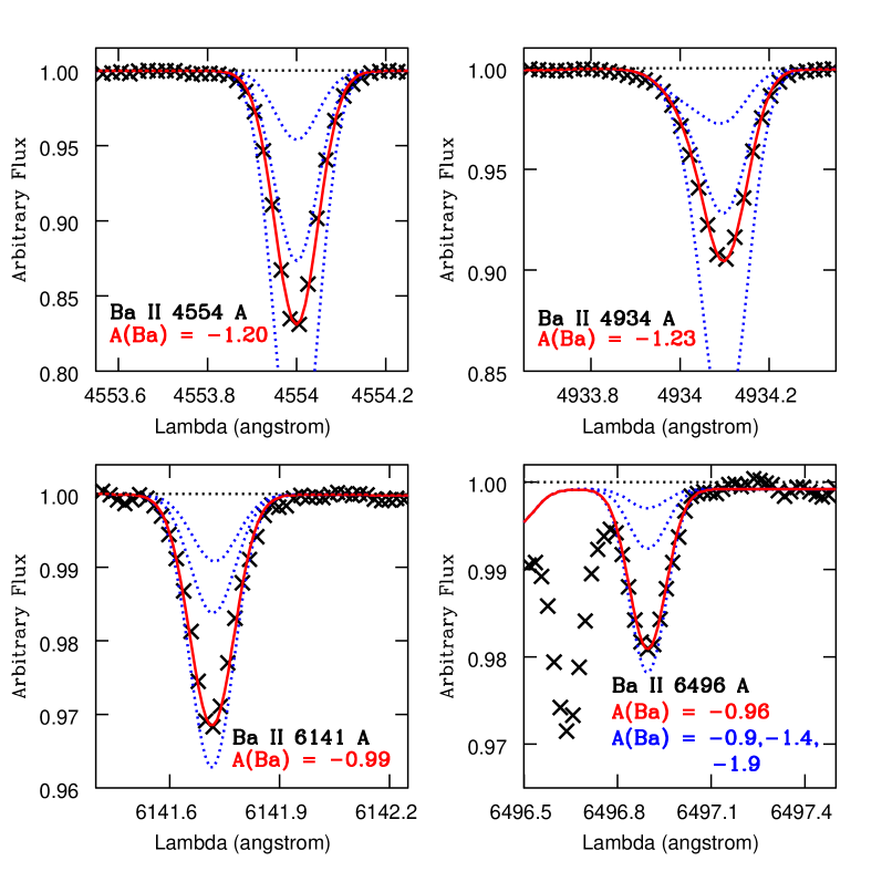
Figure 6: LTE barium abundance in HD 140283 from Ba II 4554.03 Å (upper left panel), Ba II 4934.08 Å (upper right panel), Ba II 6141.71 Å (lower left panel), and Ba II 6496.90 Å (lower right panel) lines. Symbols are the same as in Fig. 3.

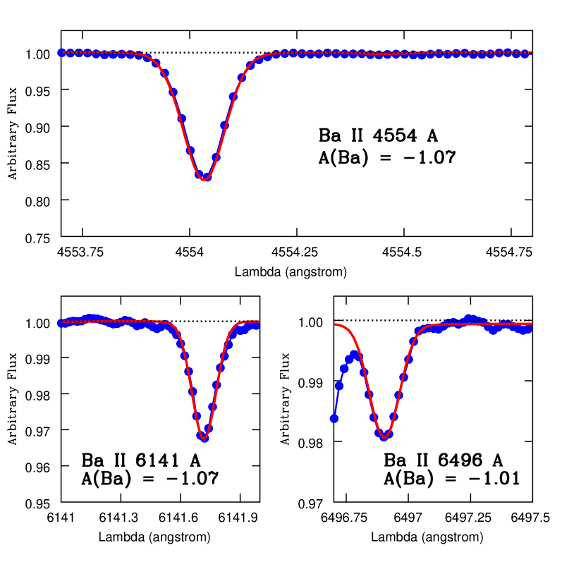
Figure 27: NLTE barium abundance in HD 140283 from Ba II 4554.03 Å (upper panel), Ba II 6141.70 Å (lower left panel), and Ba II 6496.92 Å (lower right panel) lines. Symbols are the same as in Fig. 12.

A NLTE atomic model of Ba II was presented in Andrievsky et al. (2009). Three Ba II lines were analysed in HD 140283: 4554.00 Å, 6141.70 Å, and 6496.92 Å (see Fig. 27). We applied the odd-to-even isotopic ratio 50:50, which is applicable to old metal deficient stars, to synthesize the Ba II 4554.00 Å line.

$Lanthanum$. For lanthanum, available transitions are too weak to enable us to derive a robust value for the La abundance, but the upper limit of LTE abundance A(La II) $<-1.85$ was estimated from the La II 4123.22 Å line (see upper panel in Fig. 7). This profile is located in the red wing of the H$\delta$ line, accounted for in the spectrum synthesis. We only used the major La isotope, with nuclear spin I $=7/2$, and the hyperfine coupling constants adopted basically from Lawler et al. (2001), but also from Furmann et al. (2008) and Honle et al. (1982) when not in the basic reference. We also adopted experimental oscillator strengths from Lawler et al. (2001).

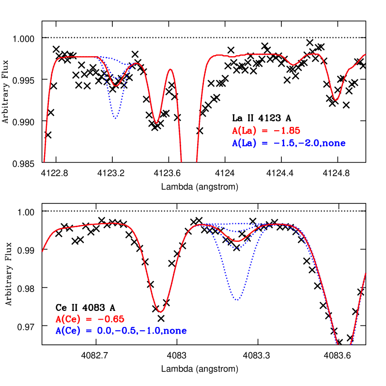
Figure 7: LTE lanthanum abundance in HD 140283 from La II 4123.22 Å line (upper panel) and cerium abundance in from Ce II 4083.22 Å line (lower panel). Symbols are the same as in Fig. 3.

$Cerium$. For cerium, we used the improved laboratory transition probabilities presented in Lawler et al. (2009) to derive the LTE abundance A(Ce II) $=-0.83$, based on two Ce II lines located at 4083.22 Å (lower panel in Fig. 7) and 4222.60 Å. These are well known as good abundance indicators (e.g. Hill et al. 2002). The local continuum around Ce II 4083.22 Å is defined by the blue wing of the H$\delta$ line. These lines are weak in HD 140283, but still clearly detectable as a result of the high quality of the spectrum. These two lines give [Ce/Fe] $=+0.36$ and $+0.01$, respectively, and a corresponding mean overbundance of cerium [Ce/Fe] $=+0.18$. The overabundance is therefore to be taken with caution.

$Europium$. Paper I was dedicated to derive the LTE europium abundance in HD 140283, using the isotopic fractions in the solar material (Table 4) with nuclear spin I $=5/2$. The final abundance A(Eu II) $=-2.35\pm 0.07$ was obtained from Eu II 4129.70 Å, which is consistent with the upper limit A(Eu II) $<-2.39$ estimated from the Eu II 4205.05 Å line.

5 Discussion

Table 6: Abundances in HD 140283 computed in LTE, NLTE, and final abundances adopted. Iron is only computed in LTE.

Element	--[X/Fe]H04	--[X/Fe]LTE	--[X/Fe]NLTE	--[X/Fe]adopted
Fe	$-$2.53	$-$2.59	—-	$-$2.59
Li	—-	$+$2.14	$+$2.20†	$+$2.20
C(CH)	$+$0.47	$+$0.46	—-	$+$0.46
C(CI)	—-	$+$0.60	$+$0.16	$+$0.16
N(CN)	—-	$+$1.06	—-	$+$1.06
O	—-	$+$0.97	$+$0.90	$+$0.90
Na	—-	$-$0.04	$-$0.29	$-$0.29
Mg	$+$0.25	$+$0.26	$+$0.43	$+$0.43
Al	$-$0.94	$-$0.91	$-$0.17	$-$0.17
Si	$+$0.34	$+$0.38	—-	$+$0.38
K	—-	$+$0.54	$+$0.26	$+$0.26
Ca	$+$0.33	$+$0.27	$+$0.42	$+$0.42
Sc	$+$0.10	$+$0.10	—-	$+$0.10
Ti	$+$0.36	$+$0.33	—-	$+$0.33
V	$+$0.21	$+$0.22	—-	$+$0.22
Cr	$+$0.30	$+$0.08	—-	$+$0.08
Mn	$-$0.25	$-$0.29	—-	$-$0.29
Co	$+$0.25	$+$0.29	—-	$+$0.29
Ni	$+$0.13	$+$0.12	—-	$+$0.12
Zn	—-	$+$0.25	—-	$+$0.25
Ge	—-	—-	—-	$<-$0.46
As	—-	—-	—-	$+$0.381
Se	—-	—-	—-	$-$0.151
Sr	$-$0.31	$-$0.18	$-$0.30	$-$0.30
Y	$-$0.46	$-$0.40	—-	$-$0.40
Zr	$-$0.14	$-$0.07	—-	$-$0.07
Mo	—-	—-	—-	$+$0.192
Ru	—-	—-	—-	$<+$0.992
Ba	$-$0.96	$-$0.81	$-$0.63	$-$0.63
La	—-	$<-$0.36	—-	$<-$0.36
Ce	—-	$+$0.18	—-	$+$0.18
Eu	—-	$-$0.28	—-	$-$0.28
Pt	—-	—-	—-	$<+$0.371
Pb	—-	—-	—-	$<+$1.541

H04: Honda et al. (2004a,b); LTE: this work, in LTE; NLTE: this work, in NLTE. $\dagger$: based on the NLTE corrections from Asplund et al. (2006). References: 1 Roederer (2012); 2 Peterson (2011).

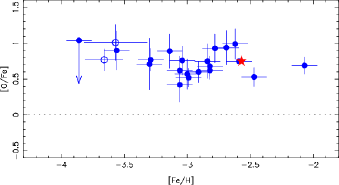
Figure 8: Comparison of the LTE [O/Fe] ratio obtained for the giant stars in the Large Programme “First Stars” based on the forbidden [O I] 6300.31 Å line (blue filled dots) and in HD 140283 (red star). The blue open circles represent the two componnents of the turnoff binary CS 22876-032.

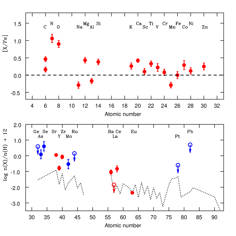
Figure 9: Abundance pattern of HD 140283 based on the present results (red circles) and literature (blue circles). The dotted line is the abundance pattern of CS 31082-001, an r-II EMP star, representing the expected abundances for an r-rich star, rescaled to match the Eu abundance in HD 140283.

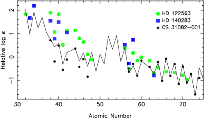
Figure 10: Comparison of the abundance pattern of HD 140283, based on the present results and literature (blue squares), with the pattern of HD 122563 (green circles) and CS 31082-001 (black dots). The solid line is the residual solar r-process pattern.

In Table 6 we present the abundances derived in LTE for 25 elements and an upper limit for lanthanum along with abundances derived in NLTE for 9 elements, and the final abundances adopted. This table also includes abundances from Honda et al. (2004a) and abundances, for As, Se, Pt, Pb, from Roederer (2012) and, Mo and Ru, from Peterson (2011). All of these are scaled to the metallicity and solar abundances adopted in this analysis.

We adopted as final abundances those analysed with NLTE models (Table 5), for the nine elements studied in NLTE, otherwise we adoted the LTE results. The LTE abundances for Sc, V, and Cr are the average from neutral and ionized lines. For Mg II, Si II, and Ca II, for which individual lines are reported in Table A, the number of useful lines are too small in comparison with the neutral species, so we did not include them in the average results.

5.1 Comparison with the literature

The forbidden [O I] 6300.31 Å line is considered the best oxygen abundance indicator, given that it is not affected by NLTE effects. We derive an abundance of A(O) $=+6.95$. The triplet lines at 7774-7 Å and 8446 Å computed in NLTE give an oxygen abundance A(O) $=+7.02$, and [O/Fe] $=+0.90$ was derived for HD 140238. Note that Fe was only computed in LTE. Meléndez et al. (2006) found a difference of $\Delta$Fe${}_{NLTE-LTE}=+0.08$ dex, which would reduce the oxygen overabundance to [O/Fe] $=+0.82$. This absolute oxygen abundance is in rather good agreement with previous NLTE derivation by Meléndez et al. (2006) of A(O) $=+6.97$, and [O/Fe] $=+0.57$, where the difference in oxygen to iron is due to their metallicity of [Fe/H] $=-2.25$ value (in NLTE), higher by $0.34$ dex than the present value of [Fe/H] $=-2.59$. Values of [Fe/H] $=-2.3$, [O/H] $=-1.67$ and [O/Fe] $=+0.7$ were adopted by Bond et al. (2013).

In Fig. 8 we present a comparison of the LTE [O/Fe] abundance ratios obtained for the giant stars analysed in the Large Programme “First Stars” (Cayrel et al. 2004; Spite et al. 2005) based on the forbidden [O I] 6300.31 Å line, with the result derived for HD 140283. We computed [O/Fe] in HD 140283, adopting the solar oxygen abundance A(O) $=+8.77$ for compatibility with the Large Programme. The [O/Fe] ratio obtained in the two components of the well-known spectroscopic turnoff binary CS 22876-032 (González Hernández et al. 2008) from the OH band, which includes corrections for 3D effects, are also presented.

The high nitrogen abundance of [N/Fe] $=+1.06$, and a consequent high [C+N+O/Fe] abundance ratio confirms previous findings by Barbuy (1983).

The results from Honda et al. (2004a) reported in Table 6 were derived from a high-resolution and high-S/N spectrum obtained with the Subaru High Dispersion Spectrograph. The Cr abundance is the only result significantly different from ours for which the present value is $0.22$ dex lower in comparison with their result. In both cases the abundance is the average of Cr I and Cr II lines. Honda et al. (2004a) adopted a $T_{\mathrm{eff}}$ 120 K lower and a gravity log $g$ 0.2 dex lower with respect to our set of parameters, whereas they used the same value for microturbulence, which is the most important error source in Cr abundance. However, their Cr abundance was derived only based on three lines, in comparison with 33 lines in the present work, which we consider a more reliable final abundance.

Roederer (2012) analysed the zinc abundance in HD 140283 based on two Zn I lines also used in the present work, with a spectrum obtained with HARPS/ESO, deriving a result $0.08$ dex lower in comparison with our abundance. However, the signal-to-noise ratio achieved in the present work is much higher than the value from Roederer (2012) (250 at 4500 Å), leading us to adopt the present result as the final Zn abundance. In addition, Roederer (2012) was able to use the UV Zn II line located at 2062.00 Å with a spectrum obtained with STIS/HST to derive A(Zn II) $=+2.27$, or [Zn II/Fe] $=+0.30$, which is higher than the result from neutral transitions.

For strontium, the LTE result of [Sr II/Fe] $=-0.17$ derived here agrees with the result from Roederer (2012), which used the same two Sr II lines, but with log $gf$ $=+0.15$ for Sr II 4077.7 Å, slightly lower than the adopted value. On the other hand, this value is higher in comparison with the LTE results from Honda et al. (2004a). Our adopted NLTE analysis gives [Sr II/Fe] $=-0.30$.

The yttrium abundance was derived in Honda et al. (2004a,b) based on three Y II lines, located at 3788.70 Å, 3950.35 Å, and 4883.69 Å. We added another two Y II lines and the derived abundance [Y II/Fe] $=-0.40$ is slightly higher than the result from Honda et al. (2004a,b), and it is in very good agreement with the abundance derived in Peterson (2011).

The zirconium abundance we derived is $0.1$ dex higher than the result from Honda et al. (2004a,b), where two Zr II lines located at 3836.76 Å and 4208.98 Å were analysed. We adopted the same values of oscillator strengths, and also used an extra Zr II line located at 4443.01 Å, with individual abundances in agreement with the result from the 4208.98 Å line. Roederer (2012) also obtained a Zr abundance $0.1$ dex lower than the present result, using the Zr II lines at 3998.96 Å, 4149.20 Å, and 4208.98 Å, in common with our analysis. For the latter line, Roederer (2012) obtained A(Zr II) $=-0.09$, only $0.04$ dex lower than the present result. In our spectrum the lines 3998.96 Å and 4149.20 Å appear severely blended and they were excluded. In addition, Peterson (2011) derived an intermediate Zr abundance between the present value and that from Roederer (2012), in agreement with our result within error bars.

5.2 Source of neutron-capture elements

Truran (1981) suggested an early enrichment of heavy elements uniquely through the r-process, arguing that there would be no time for the s-process to operate before the formation of the oldest stars. In this scenario, even dominantly s-process elements such as Sr, Y, Zr, and Ba, would have been produced by the r-process in their relatively reduced amounts.

Given the recent discussions on the r-process or s-process origin of the heavy elements in HD 140283, below we try to understand the results concerning this star. Since HD 140283 is one of the oldest stars known so far, formed shortly after the Big Bang, it is a natural test star for studies of early heavy element formation.

As described in Paper I, the barium isotopic abundances in HD 140283 are subject to intense debate in the literature. In a 1D LTE study of barium isotopes, Gallagher et al. (2010, 2012) found isotope ratios close to the s-process-only composition. This is supported by Collet et al. (2009), using 3D hydrodynamical models, where a maximum fraction of 15$\pm$34% contribution of the r-process to the isotopic mix in HD 140283 is derived. More recently, Gallagher et al. (2015) carried out 3D calculations of the barium isotopic lines in HD 140283, and the authors now favour a dominant r-process signature imprinted in the barium isotopes in HD 140283. Gallagher et al. (2015) suggest that further work is needed to improve the line formation in 3D, and that NLTE has to be taken into account.

The [Eu/Ba] ratio is the unambigous indicator as to whether the heavy elements in HD 140283 are dominantly r- or s-process. In Paper I we concluded that the [Eu/Ba] $=+0.58\pm 0.15$ value indicates that r-process is the dominant nucleosynthesis process. We found an LTE Ba abundance A(Ba) $=-1.22$, in agreement within errors with A(Ba) $=-1.28$ from 1D calculations in LTE derived by Gallagher et al. (2015). With the newly derived Ba abundance, the ratio [Eu/Ba] $=+0.53\pm 0.18$ confirms the previous conclusion concerning the dominant r-process origin.

An NLTE Ba abundance A(Ba) $=-1.05$, or [Ba II/Fe] $=-0.63$ is derived here, and a lower [Eu/Ba] $=+0.34$ ratio is obtained in this case. If an NLTE Ba abundance is considered, NLTE Eu also has to be considered: Mashonkina et al. (2012) presented NLTE abundance corrections for the Eu II 4129 Å line in cool stars, showing that the corrections are small (lower than 0.1 dex) and positive for this element and these types of stars, which would turn the present [Eu/Ba]$\approx$0.44. A further ingredient is 3D vs. 1D calculations: Gallagher et al. (2015) reported A(Ba) $=-1.43$ in HD 140283 from LTE 3D calculations, therefore, with a $0.15$ dex lower value for the 3D with respect to 1D calculations, and in this case LTE [Eu/Ba(3D)] $=+0.74$ is obtained, or else adding the 3D effect to [Eu/Ba]$\approx$0.44 above, gives [Eu/Ba]$\approx$0.59. In Table 7 we try to summarize all [Eu/Ba] values given above.

According to Simmerer et al. (2004), a pure r-process contribution gives [Eu/Ba]${}_{r}=+0.698$, whereas [Eu/Ba]${}_{s}=-1.621$ is the abundance pattern due to the pure s-process. Recent models for the solar s-process abundances (Bisterzo et al. 2014) predict the same contribution for Ba in comparison with Simmerer et al. (2004), and a slightly higher contribution for the Eu abundance: 2.7% from Simmerer et al. (2004); 6.0$\pm$0.4% from Bisterzo et al. (2014). In conclusion, the abundance ratios [Eu/Ba] described above do not change significantly.

If a lower [Eu/Ba] value relative to Paper I is confirmed, it may indicate that the contribution from the s-process to the heavy elements is not so small. Table 7 shows that no clear conclusion can be reached, but that conclusions from Paper I are still favoured. This discussion indicates that a robust 3D+NLTE synthesis is needed to enable further conclusions.

Table 7: [Eu/Ba] abundance ratios expected from the r- and s-process, and derived in HD 140283.

Source	[Eu/Ba]
†pure r-process	$+$0.698
†pure s-process	$-$1.621
Eu1D+LTE $+$ Ba1D+LTE	$+$0.53
Eu1D+LTE $+$ Ba1D+NLTE	$+$0.34
Eu1D+LTE $+$ △Ba3D+LTE	$+$0.74
♢Eu1D+NLTE $+$ Ba1D+NLTE	$+$0.44
♢Eu1D+NLTE $+$ △Ba3D+NLTE	$+$0.59

$\dagger$: Simmerer et al. (2004); $\triangle$: 3D correction from Gallagher et al. (2015); $\diamondsuit$: NLTE correction from Mashonkina et al. (2012).

5.2.1 Abundance pattern

Figure 9 shows the abundance pattern of HD 140283, based on values derived in the present work (red circles), as well as results from the literature (blue circles), where upper limits are also indicated. The upper panel presents the elements from carbon to zinc, where carbon from both CH and C I lines are indicated. The neutron-capture elements are shown in the lower panel. As a reference abundance pattern, we used the r-element enhanced EMP (r-II) star CS 31082-001 (Barbuy et al. 2011; Siqueira-Mello et al. 2013) for comparison (dotted line), rescaled to match the dominantly r-process europium abundance in HD 140283. This figure shows the overabundance of the lighter heavy elements (including Sr, Y, and Zr) in comparison with expected values from an r-rich star.

The LTE abundances of Ba and Sr result in [Sr/Ba] $=+0.63$ for HD 140283. If we take the LTE 3D Ba correction from Gallagher et al. (2015) into account, this value would be [Sr/Ba] $=+0.78$, even more overabundant. The newly derived NLTE abundances of Ba and Sr give [Sr/Ba] $=+0.33$, or [Sr/Ba] $=+0.48$ if the 3D Ba correction is applied. Overabundances are also obtained for Y and Zr, reaching values of [Y/Ba] $=+0.41$ and [Zr/Ba] $=+0.74$ in the present work, using only the LTE results. With the NLTE Ba abundance these ratios decrease to [Y/Ba] $=+0.23$ and [Zr/Ba] $=+0.56$ in HD 140283, but the 3D Ba correction enhances these values to [Y/Ba] $=+0.38$ and [Zr/Ba] $=+0.71$. In Table 8 these values are summarized, showing that it is important to account for NLTE and 3D effects to evaluate these abundance ratios.

Table 8: [Sr, Y, Zr/Ba] abundance ratios derived in HD 140283.

Source	Abundance
Sr1D+LTE $+$ Ba1D+LTE	[Sr/Ba] $=+$0.63
Sr1D+NLTE $+$ Ba1D+NLTE	[Sr/Ba] $=+$0.33
Sr1D+LTE $+$ △Ba3D+LTE	[Sr/Ba] $=+$0.78
Sr1D+NLTE $+$ △Ba3D+NLTE	[Sr/Ba] $=+$0.48
Y1D+LTE $+$ Ba1D+LTE	[Y/Ba] $=+$0.41
Y1D+LTE $+$ Ba1D+NLTE	[Y/Ba] $=+$0.23
Y1D+LTE $+$ △Ba3D+NLTE	[Y/Ba] $=+$0.38
Zr1D+LTE $+$ Ba1D+LTE	[Zr/Ba] $=+$0.74
Zr1D+LTE $+$ Ba1D+NLTE	[Zr/Ba] $=+$0.56
Zr1D+LTE $+$ △Ba3D+NLTE	[Zr/Ba] $=+$0.71

$\triangle$: 3D correction from Gallagher et al. (2015).

Several authors found high abundance ratios of first peak elements Sr, Y, Zr, with respect to Ba: [Sr,Y,Zr/Ba] $>0$, in very metal-poor stars (e.g. Honda et al. 2004a,b; Honda et al. 2006; François et al. 2007; Cowan et al. 2011). According to Simmerer et al. (2004), in the solar material these elements are mainly produced by the s-process, with fractions of 89%, 72%, and 81%, respectively, but recent results described in Bisterzo et al. (2014) are different for some elements (Sr: 68.9$\pm$5.9%; Y: 71.9$\pm$8.0%; Zr: 66.3$\pm$7.4%). Therefore, while a mechanism responsible for a r-II pattern is claimed to explain the nucleosynthesis of the heaviest trans-iron elements, an extra mechanism (such as truncation or other) should act to produce the enhancement of the lightest heavy elements relative to the heaviest elements, which must occur very early in the history of the Universe.

Several models in the literature find that supernova explosion explain the overabundances of the first peak elements in metal-poor stars. Montes et al. (2007) provided evidence for the existence of a light element primary process that contributes to the nucleosynthesis of most elements in the Sr to Ag range, producing early high [Sr,Y,Zr/Ba] ratios. The astrophysical scenarios in neutrino-driven winds are claimed as promising sources of light trans-iron elements (Wanajo 2013, Arcones et al. 2013). See also the LEPP (e.g. Bisterzo et al. 2014).

Hansen et al. (2014) show that the observed patterns may be obtained by combining an r- and an s-pattern, but the ’s’ has to be (slowly) produced in another generation (AGB?), not very compatible with the great age of the star. Yet, a full understanding of core collapse supernova explosion using 3D hydrodynamical modelling is needed.

A possibility that HD 140283 formed in a very early dispersed cloud could also lead to a previous early chemical enrichment or pollution by massive AGB stars, which overproduce the first peak s-process elements (Bisterzo et al. 2010). In this scenario, a previous enrichment in Fe seeds is needed, and the timescale of the whole process is too long and not ideal for such an old star.

In Fig. 10 we show the abundance pattern in HD 140283 (blue squares) compared with the values obtained in HD 122563 (green circles), a metal-poor star well-known for its excesses of light neutron-capture elements. The abundances of the heavy elements in HD 122563 have been taken from Honda et al. (2006), Cowan et al. (2005), and Roederer et al. (2010). As references, we included the abundances of CS 31082-001 (black dots) and the residual solar r-process pattern, following the deconvolution by Simmerer et al. (2004). The data were rescaled to match the europium abundances. The overabundance of first peak elements derived in HD 140283 are only slighly lower than the values observed in HD 122563.

In conclusion, Figures 9 and 10 show overabundances of the first-peak heavy elements, and, at a lower level, also of Ba, La and Ce, with respect to CS 31082-001 and the residual solar r-process. It is not clear if the extra mechanism claimed to explain the higher abundances of light neutron-capture elements might also produce heavier elements, but less efficiently.

The overabundance of cerium [Ce/Fe] $=+0.18$, a dominantly s-process element (83.5$\pm$5.9% in the solar material, from Bisterzo et al. 2014), was also found in other few stars. In François et al. (2007), the star CS 30325-094 also showed a high Ce overabundance [Ce/Fe] $=+0.43$, however, with deficient values for other s-elements like Ba ([Ba/Fe] $=-1.88$) and Sr ([Sr/Fe] $=-2.24$). In Fig. 9 and 10 the Ce abundance in HD 140283 is clearly higher than the r-process pattern, and the same behaviour is observed in HD 122563. Because of the difficulty in explaining the abundance pattern of HD 122563 as a combination of the r-process and the main s-process, Honda et al. (2006) suggested a single process that is responsible for the enhancement of the light neutron-capture elements and the production of heavy elements in this star. A truncation process in the initial supernova (Aoki et al. 2013) could be a possible solution. A new model of hypernova shows that the explosion correctly produces the abundances of the elements observed in HD 122563, therefore, explaining the so-called weak r-process (Fujibayashi et al. 2015) as well as the similar pattern derived in HD 140283.

6 Conclusions

We used a high-S/N and high-resolution spectrum of HD 140283, obtained with a seven hour exposure with the ESPaDOnS spectrograph at the CFHT telescope, to provide a line list for metal-poor subgiant stars of which HD 140283 is a template. We carried out a detailed derivation of abundances, using both LTE and NLTE calculations, based on as many as possible reliable lines available.

In Paper I we concluded that the derived europium abundance was indicative of an r-process origin for europium. The present LTE [Eu/Ba] $=+0.53\pm 0.18$ confirms that conclusion. Combining the newly derived NLTE Ba abundance with NLTE corrections for Eu and 3D corrections for Ba from recent literature, the abundance ratio [Eu/Ba] $=+0.59\pm 0.18$ also indicates a small contribution (if any) from the main s-process to the neutron-capture elements in HD 140283.

An extra mechanism is claimed to explain the overabundances of lighter heavy elements, in addition to an r-II abundance pattern responsible for the heavier elements, and possible astrophysical scenarios are discussed. The high Ba, La, and Ce abundances derived in HD 140283 are similar to those in HD 122563, and these two stars may be excellent examples of abundances dominated by the weak r-process.

Appendix A Line lists

[x]cccrrcccc Fe and Ti lines adopted: species, wavelength (Å), excitation potential (eV), oscillator strengths from VALD and NIST, measured equivalent widths EWs (mÅ), errors on the EWs, resulting abundances and associated errors.
Species & $\lambda$(Å) $\chi$_ex(eV) log $gf_{VALD}$ log $gf_{NIST}$ EW(mÅ) $\sigma$EW(mÅ) A(X) $\sigma$A(X)
continued.
Species $\lambda$(Å) $\chi$_ex(eV) log $gf_{VALD}$ log $gf_{NIST}$ EW(mÅ) $\sigma$EW(mÅ) A(X) $\sigma$A(X)
Ti I 3989.757 0.021 $-$0.198 $-$0.126 21.37 0.73 2.73 0.02
Ti I 3998.637 0.048 $-$0.056 0.016 24.37 0.40 2.69 0.01
Ti I 4533.240 0.848 0.476 0.476 16.57 0.39 2.69 0.01
Ti I 4534.776 0.836 0.280 0.280 11.62 0.15 2.69 0.01
Ti I 4656.468 0.000 $-$1.345 $-$1.283 2.41 0.10 2.74 0.02
Ti I 4681.908 0.048 $-$1.071 $-$1.009 3.66 0.15 2.70 0.02
Ti I 4981.731 0.848 0.504 0.504 18.61 0.25 2.70 0.01
Ti I 4991.067 0.836 0.380 0.380 15.63 0.23 2.71 0.01
Ti I 4999.502 0.826 0.250 0.250 12.21 0.17 2.71 0.01
Ti I 5064.652 0.048 $-$0.991 $-$0.929 4.75 0.08 2.71 0.01
Ti I 5173.740 0.000 $-$1.118 $-$1.070 4.15 0.09 2.72 0.01
Ti I 5192.969 0.021 $-$1.006 $-$0.960 5.14 0.09 2.73 0.01
Ti I 5210.384 0.048 $-$0.884 $-$0.850 5.87 0.11 2.70 0.01
Ti II 3913.461 1.116 $-$0.410 $-$0.416 67.64 0.44 2.69 0.01
Ti II 4028.338 1.892 $-$0.960 $-$0.959 12.21 0.20 2.67 0.01
Ti II 4290.215 1.165 $-$0.930 $-$0.848 46.82 1.22 2.74 0.03
Ti II 4394.059 1.221 $-$1.770 $-$1.784 11.06 0.40 2.73 0.02
Ti II 4395.839 1.243 $-$1.970 $-$1.928 7.49 1.05 2.76 0.06
Ti II 4399.765 1.237 $-$1.220 $-$1.186 30.09 0.66 2.75 0.02
Ti II 4417.714 1.165 $-$1.230 $-$1.430 32.10 0.35 2.73 0.01
Ti II 4418.331 1.237 $-$1.990 $-$1.965 6.40 0.15 2.70 0.01
Ti II 4443.801 1.080 $-$0.700 $-$0.717 60.61 0.57 2.70 0.01
Ti II 4444.555 1.116 $-$2.210 $-$2.030 5.38 0.14 2.72 0.01
Ti II 4450.482 1.084 $-$1.510 $-$1.518 23.92 0.65 2.74 0.02
Ti II 4464.449 1.161 $-$1.810 $-$2.080 11.61 0.27 2.73 0.01
Ti II 4468.492 1.131 $-$0.600 $-$0.620 62.82 0.59 2.69 0.01
Ti II 4470.853 1.165 $-$2.060 $-$2.280 5.66 0.10 2.64 0.01
Ti II 4501.270 1.116 $-$0.760 $-$0.767 57.13 0.50 2.71 0.01
Ti II 4533.960 1.237 $-$0.540 $-$0.770 59.54 1.28 2.66 0.03
Ti II 4563.757 1.221 $-$0.790 $-$0.960 49.56 0.41 2.69 0.01
Ti II 4571.971 1.572 $-$0.320 $-$0.317 52.66 0.48 2.63 0.01
Ti II 5129.156 1.892 $-$1.240 $-$1.239 6.57 0.36 2.57 0.02
Ti II 5185.902 1.893 $-$1.490 $-$1.487 4.89 0.11 2.68 0.01
Ti II 5188.687 1.582 $-$1.050 $-$1.220 21.25 0.34 2.66 0.01
Ti II 5226.538 1.566 $-$1.260 $-$1.290 15.23 0.18 2.67 0.01
Ti II 5336.786 1.582 $-$1.590 $-$1.700 7.86 0.13 2.68 0.01
Ti II 5381.021 1.566 $-$1.920 $-$1.921 3.64 0.08 2.64 0.01
Fe I 3742.616 2.940 $-$0.894 $-$0.894 17.10 1.45 5.05 0.04
Fe I 3774.824 2.223 $-$1.447 $-$1.447 13.82 1.22 4.79 0.04
Fe I 3776.455 2.176 $-$1.493 $-$1.493 16.81 1.04 4.90 0.03
Fe I 3781.186 2.198 $-$1.940 $-$1.940 7.14 0.98 4.93 0.06
Fe I 3786.677 1.011 $-$2.225 $-$2.225 38.00 1.50 5.00 0.03
Fe I 3787.880 1.011 $-$0.859 $-$0.859 88.69 1.17 4.91 0.03
Fe I 3794.339 2.453 $-$1.006 $-$1.006 19.16 0.60 4.75 0.02
Fe I 3795.002 0.990 $-$0.761 $-$0.761 86.54 0.94 4.74 0.02
Fe I 3805.342 3.301 0.312 0.313 39.69 0.86 4.77 0.02
Fe I 3807.537 2.223 $-$0.992 $-$0.992 31.34 0.84 4.83 0.02
Fe I 3808.728 2.559 $-$1.159 $-$1.159 17.27 0.93 4.95 0.03
Fe I 3817.639 3.332 $-$0.700 $-$0.730 10.72 0.40 4.99 0.02
Fe I 3821.178 3.267 0.198 0.198 37.51 0.99 4.80 0.02
Fe I 3821.834 2.609 $-$1.097 $-$1.097 17.60 0.99 4.95 0.03
Fe I 3840.437 0.990 $-$0.506 $-$0.506 100.34 1.71 4.76 0.03
Fe I 3841.048 1.608 $-$0.045 $-$0.045 95.76 1.91 4.78 0.04
Fe I 3843.257 3.047 $-$0.241 $-$0.241 30.52 0.93 4.86 0.02
Fe I 3845.169 2.424 $-$1.394 $-$1.394 12.00 0.74 4.86 0.03
Fe I 3846.409 3.573 $-$0.475 $-$0.474 7.10 0.39 4.80 0.03
Fe I 3846.800 3.252 $-$0.016 $-$0.016 31.10 1.59 4.85 0.04
Fe I 3849.966 1.011 $-$0.871 $-$0.871 89.65 1.46 4.92 0.03
Fe I 3850.818 0.990 $-$1.734 $-$1.734 60.74 1.48 5.02 0.04
Fe I 3852.572 2.176 $-$1.185 $-$1.185 26.76 0.57 4.86 0.01
Fe I 3856.371 0.052 $-$1.286 $-$1.286 106.06 0.73 4.82 0.01
Fe I 3863.741 2.692 $-$1.416 $-$1.431 8.10 0.42 4.94 0.02
Fe I 3865.523 1.011 $-$0.982 $-$0.982 84.09 0.75 4.89 0.02
Fe I 3867.216 3.017 $-$0.451 $-$0.451 24.67 1.24 4.89 0.03
Fe I 3878.018 0.958 $-$0.914 $-$0.914 84.72 0.77 4.79 0.02
Fe I 3885.510 2.424 $-$1.085 $-$1.085 16.73 0.71 4.72 0.02
Fe I 3891.926 3.415 $-$0.734 $-$0.734 5.60 0.34 4.79 0.03
Fe I 3893.390 2.949 $-$0.602 $-$0.602 24.29 0.54 4.96 0.01
Fe I 3899.707 0.087 $-$1.531 $-$1.531 96.90 0.95 4.89 0.02
Fe I 3906.479 0.110 $-$2.243 $-$2.243 74.72 0.80 5.04 0.02
Fe I 3907.934 2.759 $-$1.117 $-$1.117 13.00 0.58 4.94 0.02
Fe I 3916.731 3.237 $-$0.584 $-$0.604 13.66 0.38 4.90 0.01
Fe I 3917.181 0.990 $-$2.155 $-$2.155 41.86 0.57 4.98 0.01
Fe I 3918.641 3.018 $-$0.725 $-$0.725 17.86 0.79 4.97 0.02
Fe I 3920.258 0.121 $-$1.746 $-$1.746 91.10 1.31 5.00 0.03
Fe I 3922.912 0.052 $-$1.651 $-$1.651 96.55 1.08 4.97 0.02
Fe I 3925.644 2.832 $-$1.032 $-$1.032 10.67 0.31 4.82 0.01
Fe I 3925.941 2.858 $-$0.936 $-$0.936 19.19 0.66 5.06 0.02
Fe I 3930.296 0.087 $-$1.491 $-$1.491 93.36 0.72 4.76 0.02
Fe I 3937.328 2.692 $-$1.459 $-$1.459 6.83 0.41 4.90 0.03
Fe I 3941.275 3.266 $-$1.010 $-$0.980 4.87 0.45 4.85 0.04
Fe I 3942.440 2.845 $-$0.951 $-$0.950 13.24 0.47 4.87 0.02
Fe I 3946.995 3.211 $-$0.998 $-$0.998 6.63 0.32 4.93 0.02
Fe I 3948.097 3.241 $-$0.560 $-$0.560 15.46 0.41 4.94 0.01
Fe I 3949.953 2.176 $-$1.251 $-$1.251 26.72 0.35 4.91 0.01
Fe I 3951.163 3.274 $-$0.299 $-$0.299 16.77 0.41 4.76 0.01
Fe I 3955.341 3.283 $-$1.010 $-$0.980 6.28 0.30 4.98 0.02
Fe I 3957.018 3.266 $-$0.562 $-$0.562 15.71 0.39 4.97 0.01
Fe I 3977.741 2.198 $-$1.119 $-$1.119 30.11 0.31 4.88 0.01
Fe I 3985.387 3.301 $-$0.993 $-$0.993 3.76 0.19 4.75 0.02
Fe I 3997.392 2.728 $-$0.479 $-$0.479 35.56 0.70 4.88 0.02
Fe I 3998.052 2.692 $-$0.910 $-$0.910 21.60 0.42 4.94 0.01
Fe I 4005.242 1.557 $-$0.610 $-$0.610 78.47 1.08 4.87 0.03
Fe I 4007.272 2.759 $-$1.276 $-$1.276 7.84 0.29 4.84 0.02
Fe I 4009.713 2.223 $-$1.252 $-$1.252 25.27 0.27 4.92 0.01
Fe I 4021.866 2.759 $-$0.729 $-$0.729 23.94 0.35 4.88 0.01
Fe I 4024.725 3.241 $-$0.753 $-$0.752 10.34 0.25 4.92 0.01
Fe I 4030.488 3.211 $-$0.555 $-$0.555 15.53 0.44 4.90 0.01
Fe I 4063.594 1.557 0.062 0.062 105.47 1.36 4.76 0.02
Fe I 4073.762 3.266 $-$0.902 $-$0.902 7.27 0.14 4.92 0.01
Fe I 4079.838 2.858 $-$1.360 $-$1.360 5.72 0.20 4.87 0.02
Fe I 4098.176 3.241 $-$0.879 $-$0.879 6.76 0.16 4.83 0.01
Fe I 4107.488 2.832 $-$0.879 $-$0.879 18.38 0.26 4.94 0.01
Fe I 4118.545 3.573 0.215 0.215 28.95 0.40 4.85 0.01
Fe I 4120.206 2.990 $-$1.267 $-$1.267 6.42 0.13 4.95 0.01
Fe I 4121.802 2.832 $-$1.450 $-$1.450 6.83 0.15 5.01 0.01
Fe I 4132.058 1.608 $-$0.675 $-$0.675 77.88 1.09 4.94 0.03
Fe I 4132.899 2.845 $-$1.006 $-$1.006 15.31 0.33 4.98 0.01
Fe I 4134.677 2.832 $-$0.649 $-$0.649 26.79 0.42 4.94 0.01
Fe I 4136.997 3.415 $-$0.453 $-$0.452 10.28 0.20 4.78 0.01
Fe I 4139.927 0.990 $-$3.629 $-$3.629 2.72 0.12 4.94 0.02
Fe I 4143.414 3.047 $-$0.204 $-$0.204 34.04 0.70 4.86 0.02
Fe I 4143.868 1.557 $-$0.511 $-$0.511 83.25 0.87 4.86 0.02
Fe I 4147.669 1.485 $-$2.104 $-$2.104 22.53 0.28 4.95 0.01
Fe I 4152.169 0.958 $-$3.232 $-$3.232 8.71 0.72 5.05 0.04
Fe I 4153.900 3.397 $-$0.321 $-$0.321 18.17 0.73 4.92 0.02
Fe I 4154.498 2.832 $-$0.688 $-$0.688 22.97 1.16 4.87 0.03
Fe I 4154.805 3.368 $-$0.400 $-$0.400 17.16 0.31 4.94 0.01
Fe I 4156.799 2.832 $-$0.809 $-$0.808 22.82 0.92 4.99 0.02
Fe I 4157.780 3.417 $-$0.403 $-$0.403 14.31 0.46 4.89 0.02
Fe I 4175.636 2.845 $-$0.827 $-$0.827 20.73 0.31 4.97 0.01
Fe I 4176.566 3.368 $-$0.805 ——– 11.50 0.22 5.13 0.01
Fe I 4181.754 2.832 $-$0.371 $-$0.371 38.36 0.61 4.92 0.01
Fe I 4182.382 3.017 $-$1.180 $-$1.180 5.73 0.10 4.83 0.01
Fe I 4184.891 2.832 $-$0.869 $-$0.869 16.72 0.21 4.87 0.01
Fe I 4187.039 2.449 $-$0.548 $-$0.548 46.37 0.58 4.85 0.01
Fe I 4187.795 2.425 $-$0.554 $-$0.554 48.61 0.65 4.88 0.01
Fe I 4191.430 2.469 $-$0.666 $-$0.666 38.74 0.40 4.84 0.01
Fe I 4195.329 3.332 $-$0.492 $-$0.492 16.15 0.72 4.96 0.02
Fe I 4196.208 3.397 $-$0.696 $-$0.696 8.81 0.27 4.92 0.02
Fe I 4199.095 3.047 0.155 0.156 48.24 0.53 4.82 0.01
Fe I 4200.924 3.397 $-$0.827 $-$0.827 4.91 0.13 4.78 0.01
Fe I 4202.029 1.485 $-$0.708 $-$0.708 79.76 1.04 4.90 0.03
Fe I 4203.985 2.845 $-$1.010 $-$1.010 16.11 0.33 5.00 0.01
Fe I 4210.343 2.482 $-$0.928 $-$0.928 30.98 0.42 4.95 0.01
Fe I 4213.647 2.845 $-$1.290 $-$1.250 6.46 0.16 4.83 0.01
Fe I 4216.183 0.000 $-$3.356 $-$3.356 36.01 0.37 5.02 0.01
Fe I 4217.545 3.430 $-$0.484 $-$0.484 12.13 0.24 4.90 0.01
Fe I 4219.360 3.573 0.000 0.000 23.40 0.38 4.92 0.01
Fe I 4220.341 3.071 $-$1.311 $-$1.311 3.93 0.19 4.84 0.02
Fe I 4222.213 2.450 $-$0.967 $-$0.967 28.60 0.24 4.90 0.00
Fe I 4224.171 3.368 $-$0.506 $-$0.506 13.73 0.22 4.92 0.01
Fe I 4225.454 3.417 $-$0.510 $-$0.510 12.82 0.32 4.94 0.01
Fe I 4233.602 2.482 $-$0.604 $-$0.604 43.12 0.62 4.87 0.01
Fe I 4235.937 2.425 $-$0.341 $-$0.341 57.48 0.55 4.84 0.01
Fe I 4238.810 3.397 $-$0.233 $-$0.233 19.40 0.40 4.86 0.01
Fe I 4247.425 3.368 $-$0.239 $-$0.239 22.47 0.58 4.92 0.01
Fe I 4250.119 2.469 $-$0.405 $-$0.405 52.17 0.63 4.84 0.01
Fe I 4250.787 1.557 $-$0.714 $-$0.714 76.42 0.91 4.88 0.02
Fe I 4260.474 2.399 0.109 0.077 75.77 1.32 4.74 0.03
Fe I 4271.760 1.485 $-$0.164 $-$0.164 102.25 1.79 4.83 0.03
Fe I 4282.403 2.176 $-$0.779 $-$0.779 46.68 0.74 4.85 0.02
Fe I 4325.762 1.608 0.006 0.006 101.33 2.76 4.75 0.05
Fe I 4337.046 1.557 $-$1.695 $-$1.695 33.69 0.32 4.86 0.01
Fe I 4352.734 2.223 $-$1.287 $-$1.287 25.17 0.62 4.92 0.02
Fe I 4375.930 0.000 $-$3.031 $-$3.031 53.28 0.53 5.05 0.01
Fe I 4383.545 1.485 0.200 0.200 122.49 2.23 4.76 0.03
Fe I 4388.407 3.602 $-$0.682 $-$0.682 6.67 0.22 4.96 0.02
Fe I 4404.750 1.557 $-$0.142 $-$0.142 100.59 1.42 4.82 0.03
Fe I 4415.122 1.608 $-$0.615 $-$0.615 81.79 1.02 4.93 0.02
Fe I 4427.310 0.052 $-$2.924 $-$3.044 52.82 1.09 4.98 0.03
Fe I 4430.614 2.223 $-$1.659 $-$1.659 13.27 0.24 4.92 0.01
Fe I 4442.339 2.198 $-$1.255 $-$1.255 29.20 0.39 4.94 0.01
Fe I 4443.194 2.858 $-$1.043 $-$1.043 12.05 0.21 4.88 0.01
Fe I 4447.717 2.223 $-$1.342 $-$1.342 24.09 0.26 4.93 0.01
Fe I 4454.381 2.831 $-$1.299 $-$1.299 8.18 0.19 4.92 0.01
Fe I 4461.653 0.087 $-$3.210 $-$3.210 40.26 0.49 5.03 0.01
Fe I 4466.551 2.832 $-$0.600 $-$0.600 28.88 0.30 4.91 0.01
Fe I 4469.375 3.654 $-$0.477 $-$0.477 9.74 0.29 4.98 0.01
Fe I 4476.018 2.845 $-$0.819 $-$0.819 27.47 0.33 5.10 0.01
Fe I 4484.220 3.603 $-$0.864 $-$0.864 5.86 0.20 5.08 0.01
Fe I 4489.739 0.121 $-$3.966 $-$3.966 10.98 0.20 5.02 0.01
Fe I 4494.563 2.198 $-$1.136 $-$1.136 33.59 0.36 4.91 0.01
Fe I 4528.614 2.176 $-$0.822 $-$0.822 49.46 0.82 4.90 0.02
Fe I 4531.148 1.485 $-$2.155 $-$2.155 22.05 0.46 4.95 0.01
Fe I 4547.847 3.547 $-$1.012 $-$1.012 4.45 0.14 5.04 0.01
Fe I 4592.651 1.557 $-$2.449 $-$2.449 12.08 0.20 4.99 0.01
Fe I 4602.941 1.485 $-$2.209 $-$2.220 20.65 0.36 4.96 0.01
Fe I 4607.646 3.266 $-$1.467 ——– 3.23 0.14 5.07 0.02
Fe I 4619.288 3.603 $-$1.120 $-$1.080 2.81 0.12 4.99 0.02
Fe I 4625.045 3.241 $-$1.340 ——– 3.28 0.17 4.93 0.02
Fe I 4632.911 1.608 $-$2.913 $-$2.913 4.12 0.16 4.99 0.02
Fe I 4637.503 3.283 $-$1.390 $-$1.340 3.37 0.11 5.03 0.01
Fe I 4638.010 3.603 $-$1.119 $-$1.119 2.94 0.12 5.01 0.02
Fe I 4647.434 2.949 $-$1.351 $-$1.351 6.15 0.13 4.94 0.01
Fe I 4668.134 3.266 $-$1.210 ——– 5.16 0.14 5.03 0.01
Fe I 4678.846 3.603 $-$0.833 $-$0.833 6.50 0.13 5.08 0.01
Fe I 4707.274 3.241 $-$1.080 ——– 7.42 0.49 5.04 0.03
Fe I 4733.591 1.485 $-$2.988 $-$2.987 4.57 0.10 4.98 0.01
Fe I 4736.773 3.211 $-$0.752 $-$0.752 13.49 0.15 4.97 0.01
Fe I 4789.651 3.547 $-$0.958 $-$0.958 3.82 0.17 4.90 0.02
Fe I 4871.318 2.865 $-$0.363 $-$0.362 36.07 0.48 4.82 0.01
Fe I 4872.138 2.882 $-$0.567 $-$0.567 27.10 0.40 4.85 0.01
Fe I 4890.755 2.876 $-$0.394 $-$0.394 35.57 0.61 4.85 0.01
Fe I 4891.492 2.851 $-$0.112 $-$0.112 49.75 0.85 4.82 0.02
Fe I 4903.310 2.882 $-$0.926 $-$0.926 15.62 0.21 4.89 0.01
Fe I 4918.994 2.865 $-$0.342 $-$0.342 38.12 0.42 4.84 0.01
Fe I 4920.503 2.833 0.068 0.068 58.75 0.85 4.79 0.02
Fe I 4924.770 2.279 $-$2.241 $-$2.114 4.49 0.10 5.01 0.01
Fe I 4938.814 2.876 $-$1.077 $-$1.077 11.74 0.21 4.89 0.01
Fe I 4939.686 0.859 $-$3.340 $-$3.340 8.91 0.14 5.00 0.01
Fe I 4946.388 3.368 $-$1.170 ——– 4.00 0.10 4.96 0.01
Fe I 4957.298 2.851 $-$0.408 $-$0.408 36.61 0.37 4.86 0.01
Fe I 4957.596 2.808 0.233 0.233 68.92 1.14 4.80 0.02
Fe I 4966.089 3.332 $-$0.871 $-$0.871 8.80 0.18 4.99 0.01
Fe I 4982.500 4.103 0.156 ——– 9.85 0.25 4.77 0.01
Fe I 4983.250 4.154 $-$0.122 ——– 5.37 0.09 4.81 0.01
Fe I 4983.853 4.103 $-$0.006 ——– 7.52 0.22 4.80 0.01
Fe I 4985.253 3.929 $-$0.560 $-$0.560 5.01 0.14 4.99 0.01
Fe I 4985.547 2.865 $-$1.332 $-$1.331 6.47 0.15 4.84 0.01
Fe I 4994.129 0.915 $-$3.080 $-$3.080 13.01 0.14 4.98 0.01
Fe I 5001.863 3.882 0.010 $-$0.010 12.84 0.26 4.83 0.01
Fe I 5006.119 2.833 $-$0.638 $-$0.615 27.47 0.40 4.87 0.01
Fe I 5012.068 0.859 $-$2.642 $-$2.642 31.79 0.53 5.01 0.01
Fe I 5014.942 3.943 $-$0.303 $-$0.303 7.94 0.11 4.97 0.01
Fe I 5022.235 3.984 $-$0.530 $-$0.560 4.84 0.14 5.00 0.01
Fe I 5041.071 0.958 $-$3.087 $-$3.087 13.36 0.26 5.05 0.01
Fe I 5041.756 1.485 $-$2.203 $-$2.203 21.54 0.47 4.95 0.01
Fe I 5049.819 2.279 $-$1.355 $-$1.355 21.97 0.32 4.91 0.01
Fe I 5051.634 0.915 $-$2.795 $-$2.795 22.35 0.26 4.99 0.01
Fe I 5065.018 4.256 0.005 ——– 6.23 0.56 4.84 0.04
Fe I 5074.748 4.220 $-$0.200 $-$0.230 7.74 0.29 5.12 0.02
Fe I 5078.975 4.301 $-$0.292 ——– 4.71 0.29 5.06 0.03
Fe I 5079.740 0.990 $-$3.220 $-$3.220 8.32 0.28 4.97 0.02
Fe I 5083.338 0.958 $-$2.958 $-$2.958 15.40 0.16 4.99 0.01
Fe I 5098.698 2.176 $-$2.026 $-$2.026 9.82 0.30 5.05 0.01
Fe I 5110.413 0.000 $-$3.760 $-$3.760 24.41 0.32 5.08 0.01
Fe I 5123.720 1.011 $-$3.068 $-$3.068 11.22 0.15 4.99 0.01
Fe I 5127.359 0.915 $-$3.307 $-$3.307 8.73 0.10 5.01 0.00
Fe I 5150.839 0.990 $-$3.003 $-$3.037 9.78 0.12 4.83 0.01
Fe I 5151.911 1.011 $-$3.322 $-$3.322 6.51 0.21 4.98 0.02
Fe I 5162.273 4.178 0.020 ——– 11.83 0.15 5.06 0.01
Fe I 5166.282 0.000 $-$4.195 $-$4.195 10.23 0.11 5.04 0.00
Fe I 5171.596 1.485 $-$1.793 $-$1.793 40.71 0.46 4.97 0.01
Fe I 5191.455 3.038 $-$0.551 $-$0.551 21.66 0.29 4.83 0.01
Fe I 5192.344 2.998 $-$0.421 $-$0.421 28.17 0.35 4.82 0.01
Fe I 5194.941 1.557 $-$2.090 $-$2.090 23.77 0.31 4.96 0.01
Fe I 5216.274 1.608 $-$2.150 $-$2.150 19.25 0.24 4.95 0.01
Fe I 5232.940 2.940 $-$0.058 $-$0.057 47.67 0.70 4.80 0.01
Fe I 5266.555 2.998 $-$0.386 $-$0.385 30.49 0.51 4.84 0.01
Fe I 5269.537 0.859 $-$1.321 $-$1.321 94.01 1.15 5.09 0.03
Fe I 5281.790 3.038 $-$0.834 $-$0.834 13.15 0.18 4.84 0.01
Fe I 5283.621 3.241 $-$0.432 $-$0.525 18.73 0.32 4.83 0.01
Fe I 5302.299 3.283 $-$0.720 $-$0.720 10.01 0.17 4.83 0.01
Fe I 5307.361 1.608 $-$2.987 $-$2.987 3.44 0.13 4.94 0.02
Fe I 5324.179 3.211 $-$0.103 $-$0.103 32.72 0.39 4.81 0.01
Fe I 5328.038 0.915 $-$1.466 $-$1.466 85.35 1.27 5.09 0.03
Fe I 5328.531 1.557 $-$1.850 $-$1.850 33.75 1.24 4.94 0.03
Fe I 5339.929 3.266 $-$0.647 $-$0.720 12.56 0.15 4.86 0.01
Fe I 5367.466 4.415 0.443 0.443 11.06 0.21 4.83 0.01
Fe I 5369.961 4.371 0.536 0.536 13.82 0.27 4.80 0.01
Fe I 5371.489 0.958 $-$1.645 $-$1.645 77.72 0.86 5.12 0.02
Fe I 5383.369 4.312 0.645 0.645 18.41 0.27 4.79 0.01
Fe I 5393.167 3.241 $-$0.715 $-$0.715 11.68 0.19 4.86 0.01
Fe I 5397.128 0.915 $-$1.993 $-$1.993 63.17 0.74 5.07 0.02
Fe I 5404.151 4.434 0.523 0.523 18.00 0.43 5.02 0.01
Fe I 5405.775 0.990 $-$1.844 $-$1.844 66.26 0.78 5.07 0.02
Fe I 5415.199 4.386 0.642 0.642 16.19 0.41 4.79 0.01
Fe I 5424.068 4.320 0.520 ——– 20.08 0.24 4.97 0.01
Fe I 5429.696 0.958 $-$1.879 $-$1.879 67.57 0.95 5.10 0.02
Fe I 5434.524 1.011 $-$2.122 $-$2.122 51.18 0.42 5.03 0.01
Fe I 5446.916 0.990 $-$1.914 $-$1.914 64.52 0.90 5.10 0.02
Fe I 5497.516 1.011 $-$2.849 $-$2.849 18.52 0.22 5.01 0.01
Fe I 5501.465 0.958 $-$3.047 $-$3.047 13.89 0.13 5.00 0.00
Fe I 5506.779 0.990 $-$2.797 $-$2.797 20.73 0.23 5.00 0.01
Fe I 5569.618 3.417 $-$0.486 $-$0.486 12.49 0.22 4.83 0.01
Fe I 5572.842 3.396 $-$0.275 $-$0.275 19.18 0.35 4.82 0.01
Fe I 5576.089 3.430 $-$1.000 $-$0.940 6.10 0.09 5.01 0.01
Fe I 5586.756 3.368 $-$0.120 $-$0.144 26.27 0.31 4.82 0.01
Fe I 5615.644 3.332 0.050 0.050 33.93 0.84 4.79 0.02
Fe I 6136.615 2.453 $-$1.400 $-$1.400 17.04 0.45 4.93 0.01
Fe I 6137.691 2.588 $-$1.403 $-$1.403 13.68 0.19 4.95 0.04
Fe I 6191.558 2.433 $-$1.417 $-$1.416 14.74 0.43 4.85 0.01
Fe I 6219.281 2.198 $-$2.433 $-$2.433 3.03 0.28 4.87 0.04
Fe I 6230.723 2.559 $-$1.281 $-$1.281 19.55 0.48 4.99 0.01
Fe I 6252.555 2.404 $-$1.687 $-$1.687 10.99 0.27 4.94 0.01
Fe I 6393.601 2.433 $-$1.432 $-$1.576 14.40 0.21 4.84 0.01
Fe I 6400.001 3.602 $-$0.290 $-$0.290 13.86 0.50 4.84 0.02
Fe I 6421.350 2.279 $-$2.027 $-$2.027 7.47 0.27 4.96 0.02
Fe I 6430.846 2.176 $-$2.006 $-$2.006 10.04 0.18 4.97 0.01
Fe I 6494.980 2.404 $-$1.273 $-$1.273 25.26 0.36 4.97 0.01
Fe II 4178.855 2.583 $-$2.500 $-$2.440 17.15 0.29 4.97 0.01
Fe II 4233.163 2.583 $-$1.900 $-$1.810 42.23 0.73 4.97 0.02
Fe II 4385.379 2.778 $-$2.680 $-$2.600 12.66 0.37 5.16 0.01
Fe II 4416.818 2.778 $-$2.410 $-$2.600 10.82 0.22 4.81 0.01
Fe II 4489.185 2.828 $-$2.970 $-$3.000 4.95 0.26 5.04 0.02
Fe II 4491.400 2.856 $-$2.700 $-$2.640 6.95 0.18 4.96 0.01
Fe II 4508.281 2.856 $-$2.250 $-$2.300 15.60 0.24 4.91 0.01
Fe II 4515.334 2.844 $-$2.450 $-$2.360 12.11 0.28 4.97 0.01
Fe II 4520.221 2.807 $-$2.600 $-$2.600 11.18 0.24 5.04 0.01
Fe II 4522.628 2.844 $-$2.030 $-$1.990 22.92 0.36 4.89 0.01
Fe II 4541.518 2.856 $-$2.790 $-$3.000 4.66 0.15 4.86 0.01
Fe II 4555.888 2.828 $-$2.160 $-$2.250 15.66 0.20 4.79 0.01
Fe II 4576.328 2.844 $-$2.920 $-$2.920 4.45 0.22 4.95 0.02
Fe II 4582.835 2.844 $-$3.090 $-$3.060 2.68 0.15 4.89 0.02
Fe II 4583.829 2.807 $-$1.860 $-$1.740 36.21 0.36 4.99 0.01
Fe II 4731.439 2.891 $-$3.000 $-$3.100 3.70 0.11 4.99 0.01
Fe II 4923.922 2.891 $-$1.320 $-$1.210 57.37 0.70 4.97 0.02
Fe II 5018.435 2.891 $-$1.220 $-$1.350 65.85 0.96 5.06 0.02
Fe II 5197.568 3.230 $-$2.100 $-$2.050 10.82 0.15 4.90 0.01
Fe II 5234.624 3.221 $-$2.230 $-$2.210 12.89 0.23 5.11 0.01

[x]cccrrrr Line list used in the present analysis: species, wavelength (Å), oscillator strengths, excitation potential (eV), and resulting abundances line by line.
Species $\lambda$(Å) $\chi$_ex(eV) log $gf$ A(X) [X/H] [X/Fe]
continued.
Species $\lambda$(Å) $\chi$_ex(eV) log $gf$ A(X) [X/H] [X/Fe]
Li I 6103.538 1.848 0.101 $+$2.07 $+$1.02 $+$3.61
Li I 6707.761 0.000 $-$0.009 $+$2.20 $+$1.15 $+$3.74
C I 8335.148 7.685 $-$0.420 $+$6.47 $-$1.96 $+$0.63
C I 9061.433 7.483 $-$0.346 $+$6.42 $-$2.01 $+$0.58
C I 9062.487 7.480 $-$0.456 $+$6.44 $-$1.99 $+$0.60
[O I] 6300.311 0.000 $-$9.716 $+$6.95 $-$1.74 $+$0.85
O I 7771.941 9.146 0.369 $+$7.12 $-$1.57 $+$1.02
O I 7774.161 9.146 0.223 $+$7.06 $-$1.63 $+$0.96
O I 7775.388 9.146 0.001 $+$7.08 $-$1.61 $+$0.98
O I 8446.359 9.521 0.236 $+$7.17 $-$1.52 $+$1.07
Na I 4982.813 2.104 $-$0.962 $+$3.50 $-$2.74 $-$0.15
Na I 5682.633 2.102 $-$0.706 $+$3.70 $-$2.54 $+$0.05
Na I 5889.950 0.000 0.108 $+$3.70 $-$2.54 $+$0.05
Na I 5895.924 0.000 $-$0.194 $+$3.66 $-$2.58 $+$0.01
Na I 8194.824 2.104 0.492 $+$3.53 $-$2.71 $-$0.12
Mg I 3829.355 2.709 $-$0.227 $+$5.20 $-$2.40 $+$0.19
Mg I 3832.304 2.712 0.125 $+$5.15 $-$2.45 $+$0.14
Mg I 3838.292 2.717 0.397 $+$5.20 $-$2.40 $+$0.19
Mg I 4057.505 4.346 $-$0.900 $+$5.33 $-$2.27 $+$0.32
Mg I 4167.271 4.346 $-$0.745 $+$5.28 $-$2.32 $+$0.27
Mg I 4571.096 0.000 $-$5.623 $+$5.30 $-$2.30 $+$0.29
Mg I 4702.991 4.346 $-$0.440 $+$5.32 $-$2.28 $+$0.31
Mg I 5172.684 2.712 $-$0.393 $+$5.22 $-$2.38 $+$0.21
Mg I 5183.604 2.717 $-$0.167 $+$5.20 $-$2.40 $+$0.19
Mg I 5528.405 4.346 $-$0.498 $+$5.34 $-$2.26 $+$0.33
Mg I 5711.088 4.346 $-$1.724 $+$5.33 $-$2.27 $+$0.32
Mg I 8806.756 4.346 $-$0.134 $+$5.42 $-$2.18 $+$0.41
Mg II 4481.126 8.864 0.749 $+$5.63 $-$1.97 $+$0.62
Mg II 4481.150 8.864 $-$0.553 $+$5.68 $-$1.92 $+$0.67
Al I 3944.006 0.000 $-$0.635 $+$2.95 $-$3.50 $-$0.91
Al I 3961.520 0.014 $-$0.333 $+$2.96 $-$3.49 $-$0.90
Si I 3905.523 1.909 $-$1.041 $+$5.30 $-$2.21 $+$0.38
Si I 4102.936 1.909 $-$3.140 $+$5.30 $-$2.21 $+$0.38
Si I 5645.613 4.930 $-$2.043 $+$5.30 $-$2.21 $+$0.38
Si I 5684.484 4.954 $-$1.553 $+$5.28 $-$2.23 $+$0.36
Si I 7034.903 5.871 $-$0.783 $+$5.32 $-$2.19 $+$0.40
Si II 6371.370 8.121 $-$0.044 $+$5.35 $-$2.16 $+$0.43
K I 7698.965 0.000 $-$0.169 $+$2.98 $-$2.05 $+$0.54
Ca I 4108.526 2.709 $-$0.824 $+$4.10 $-$2.24 $+$0.35
Ca I 4226.728 0.000 0.244 $+$3.90 $-$2.44 $+$0.15
Ca I 4283.011 1.886 $-$0.220 $+$4.13 $-$2.21 $+$0.38
Ca I 4289.367 1.879 $-$0.300 $+$4.03 $-$2.31 $+$0.28
Ca I 4302.528 1.899 0.280 $+$3.95 $-$2.39 $+$0.20
Ca I 4318.652 1.899 $-$0.211 $+$4.00 $-$2.34 $+$0.25
Ca I 4355.079 2.709 $-$0.420 $+$3.96 $-$2.38 $+$0.21
Ca I 4425.437 1.879 $-$0.357 $+$4.00 $-$2.34 $+$0.25
Ca I 4434.957 1.886 $-$0.007 $+$3.99 $-$2.35 $+$0.24
Ca I 4435.679 1.886 $-$0.517 $+$4.03 $-$2.31 $+$0.28
Ca I 4454.779 1.899 0.258 $+$3.99 $-$2.35 $+$0.24
Ca I 4455.887 1.899 $-$0.519 $+$4.04 $-$2.30 $+$0.29
Ca I 4526.928 2.709 $-$0.548 $+$4.10 $-$2.24 $+$0.35
Ca I 4578.551 2.521 $-$0.697 $+$4.06 $-$2.28 $+$0.31
Ca I 5188.844 2.933 $-$0.075 $+$4.04 $-$2.30 $+$0.29
Ca I 5261.704 2.521 $-$0.579 $+$4.02 $-$2.32 $+$0.27
Ca I 5262.241 2.521 $-$0.471 $+$4.02 $-$2.32 $+$0.27
Ca I 5265.556 2.523 $-$0.113 $+$3.99 $-$2.35 $+$0.24
Ca I 5349.465 2.709 $-$0.310 $+$4.04 $-$2.30 $+$0.29
Ca I 5512.980 2.933 $-$0.464 $+$4.05 $-$2.29 $+$0.30
Ca I 5581.965 2.523 $-$0.555 $+$4.04 $-$2.30 $+$0.29
Ca I 5588.749 2.526 0.358 $+$3.98 $-$2.36 $+$0.23
Ca I 5590.114 2.521 $-$0.571 $+$4.05 $-$2.29 $+$0.30
Ca I 5594.462 2.523 0.097 $+$3.99 $-$2.35 $+$0.24
Ca I 5601.277 2.526 $-$0.523 $+$4.01 $-$2.33 $+$0.26
Ca I 5857.451 2.933 0.240 $+$4.07 $-$2.27 $+$0.32
Ca I 6102.723 1.879 $-$0.793 $+$4.05 $-$2.29 $+$0.30
Ca I 6122.217 1.886 $-$0.316 $+$4.06 $-$2.28 $+$0.31
Ca I 6162.173 1.899 $-$0.090 $+$4.03 $-$2.31 $+$0.28
Ca I 6169.563 2.526 $-$0.478 $+$4.06 $-$2.28 $+$0.31
Ca I 6439.075 2.526 0.390 $+$3.99 $-$2.35 $+$0.24
Ca I 6455.598 2.523 $-$1.290 $+$4.00 $-$2.34 $+$0.25
Ca I 6462.567 2.523 0.262 $+$3.97 $-$2.37 $+$0.22
Ca I 6471.668 2.526 $-$0.590 $+$4.04 $-$2.30 $+$0.29
Ca I 6493.781 2.521 $-$0.109 $+$4.01 $-$2.33 $+$0.26
Ca I 6499.650 2.523 $-$0.818 $+$4.08 $-$2.26 $+$0.33
Ca I 6717.681 2.709 $-$0.524 $+$4.06 $-$2.28 $+$0.31
Ca I 7148.150 2.709 0.137 $+$4.08 $-$2.26 $+$0.33
Ca I 7326.145 2.933 $-$0.208 $+$4.05 $-$2.29 $+$0.30
Ca II 8927.356 7.050 0.811 $+$4.43 $-$1.91 $+$0.68
Sc I 4020.392 0.000 0.199 $+$0.65 $-$2.50 $+$0.09
Sc I 4023.677 0.021 0.381 $+$0.50 $-$2.65 $-$0.06
Sc II 3843.049 0.008 $-$1.730 $+$0.88 $-$2.27 $+$0.32
Sc II 4246.820 0.315 0.242 $+$0.83 $-$2.32 $+$0.27
Sc II 4294.764 0.605 $-$1.390 $+$0.80 $-$2.35 $+$0.24
Sc II 4305.711 0.595 $-$1.300 $+$0.65 $-$2.50 $+$0.09
Sc II 4314.082 0.618 $-$0.100 $+$0.82 $-$2.33 $+$0.26
Sc II 4320.745 0.605 $-$0.250 $+$0.77 $-$2.38 $+$0.21
Sc II 4324.998 0.595 $-$0.440 $+$0.76 $-$2.39 $+$0.20
Sc II 4374.462 0.618 $-$0.420 $+$0.83 $-$2.32 $+$0.27
Sc II 4400.386 0.605 $-$0.540 $+$0.82 $-$2.33 $+$0.26
Sc II 4415.544 0.595 $-$0.670 $+$0.80 $-$2.35 $+$0.24
Sc II 4431.362 0.605 $-$1.970 $+$0.75 $-$2.40 $+$0.19
Sc II 4670.406 1.357 $-$0.580 $+$0.72 $-$2.43 $+$0.16
Sc II 5031.010 1.357 $-$0.400 $+$0.68 $-$2.47 $+$0.12
Sc II 5239.811 1.455 $-$0.770 $+$0.67 $-$2.48 $+$0.11
Sc II 5526.785 1.768 0.020 $+$0.67 $-$2.48 $+$0.11
Sc II 5641.000 1.500 $-$1.130 $+$0.74 $-$2.41 $+$0.18
Sc II 5657.896 1.507 $-$0.600 $+$0.62 $-$2.53 $+$0.06
Sc II 5667.149 1.500 $-$1.310 $+$0.75 $-$2.40 $+$0.19
Sc II 5684.202 1.507 $-$1.070 $+$0.60 $-$2.55 $+$0.04
V I 4111.774 0.301 0.408 $+$1.38 $-$2.55 $+$0.04
V I 4115.176 0.287 0.071 $+$1.40 $-$2.53 $+$0.06
V I 4379.230 0.301 0.580 $+$1.42 $-$2.51 $+$0.08
V I 4389.976 0.275 0.200 $+$1.46 $-$2.47 $+$0.12
V I 4408.193 0.275 0.020 $+$1.44 $-$2.49 $+$0.10
V I 4460.291 0.301 $-$0.150 $+$1.55 $-$2.38 $+$0.21
V I 4594.124 0.069 $-$0.670 $+$1.40 $-$2.53 $+$0.06
V II 3899.128 1.805 $-$0.770 $+$1.80 $-$2.13 $+$0.46
V II 3903.252 1.476 $-$0.910 $+$1.55 $-$2.38 $+$0.21
V II 3916.404 1.428 $-$1.070 $+$1.91 $-$2.02 $+$0.57
V II 3951.957 1.476 $-$0.730 $+$1.60 $-$2.33 $+$0.26
V II 3997.110 1.476 $-$1.200 $+$1.66 $-$2.27 $+$0.32
V II 4002.928 1.428 $-$1.440 $+$1.75 $-$2.18 $+$0.41
V II 4005.702 1.817 $-$0.450 $+$1.65 $-$2.28 $+$0.31
V II 4023.377 1.805 $-$0.610 $+$1.68 $-$2.25 $+$0.34
Cr I 3908.756 1.004 $-$1.050 $+$2.97 $-$2.67 $-$0.08
Cr I 3928.639 1.004 $-$1.310 $+$3.00 $-$2.64 $-$0.05
Cr I 3963.688 2.544 0.620 $+$3.07 $-$2.57 $+$0.02
Cr I 4254.332 0.000 $-$0.090 $+$2.95 $-$2.69 $-$0.10
Cr I 4274.796 0.000 $-$0.220 $+$2.90 $-$2.74 $-$0.15
Cr I 4289.716 0.000 $-$0.370 $+$2.92 $-$2.72 $-$0.13
Cr I 4337.552 0.968 $-$1.090 $+$2.94 $-$2.70 $-$0.11
Cr I 4344.496 1.004 $-$0.650 $+$2.89 $-$2.75 $-$0.16
Cr I 4496.842 0.941 $-$1.140 $+$3.00 $-$2.64 $-$0.05
Cr I 4545.945 0.941 $-$1.370 $+$2.94 $-$2.70 $-$0.11
Cr I 4600.748 1.004 $-$1.250 $+$2.96 $-$2.68 $-$0.09
Cr I 4616.124 0.983 $-$1.190 $+$2.97 $-$2.67 $-$0.08
Cr I 4626.173 0.968 $-$1.330 $+$3.00 $-$2.64 $-$0.05
Cr I 4646.162 1.030 $-$0.740 $+$2.97 $-$2.67 $-$0.08
Cr I 4651.284 0.983 $-$1.460 $+$2.97 $-$2.67 $-$0.08
Cr I 4652.157 1.004 $-$1.040 $+$3.00 $-$2.64 $-$0.05
Cr I 4756.112 3.104 0.090 $+$3.30 $-$2.34 $+$0.25
Cr I 4789.335 2.544 $-$0.330 $+$2.85 $-$2.79 $-$0.20
Cr I 5204.511 0.941 $-$0.190 $+$2.98 $-$2.66 $-$0.07
Cr I 5206.038 0.941 0.020 $+$2.95 $-$2.69 $-$0.10
Cr I 5208.419 0.941 0.170 $+$2.95 $-$2.69 $-$0.10
Cr I 5237.351 5.662 $-$1.836 $+$3.33 $-$2.31 $+$0.28
Cr I 5247.565 0.961 $-$1.590 $+$2.92 $-$2.72 $-$0.13
Cr I 5296.691 0.983 $-$1.360 $+$2.92 $-$2.72 $-$0.13
Cr I 5298.272 0.983 $-$1.140 $+$2.90 $-$2.74 $-$0.15
Cr I 5345.801 1.004 $-$0.950 $+$2.91 $-$2.73 $-$0.14
Cr I 5348.315 1.004 $-$1.210 $+$2.89 $-$2.75 $-$0.16
Cr I 5409.772 1.030 $-$0.670 $+$2.93 $-$2.71 $-$0.12
Cr II 4558.650 4.073 $-$0.449 $+$3.15 $-$2.49 $+$0.10
Cr II 4588.199 4.071 $-$0.845 $+$3.32 $-$2.32 $+$0.27
Cr II 4634.070 4.072 $-$1.236 $+$3.40 $-$2.24 $+$0.35
Cr II 4824.127 3.871 $-$1.085 $+$3.38 $-$2.26 $+$0.33
Cr II 4848.235 3.864 $-$1.280 $+$3.33 $-$2.31 $+$0.28
Cr II 4876.399 3.854 $-$1.580 $+$3.28 $-$2.36 $+$0.23
Cr II 5313.563 4.074 $-$1.779 $+$3.35 $-$2.29 $+$0.30
Mn I 4030.753 0.000 $-$0.480 $+$2.30 $-$3.13 $-$0.54
Mn I 4033.062 0.000 $-$0.617 $+$2.29 $-$3.14 $-$0.55
Mn I 4034.483 0.000 $-$0.812 $+$2.35 $-$3.08 $-$0.49
Mn I 4041.355 2.114 0.285 $+$2.57 $-$2.86 $-$0.27
Mn I 4048.743 2.164 $-$0.130 $+$2.46 $-$2.97 $-$0.38
Mn I 4055.544 2.143 $-$0.070 $+$2.58 $-$2.85 $-$0.26
Mn I 4082.939 2.178 $-$0.354 $+$2.59 $-$2.84 $-$0.25
Mn I 4451.586 2.888 0.278 $+$2.58 $-$2.85 $-$0.26
Mn I 4458.254 3.073 0.042 $+$2.50 $-$2.93 $-$0.34
Mn I 4754.042 2.282 $-$0.086 $+$2.54 $-$2.89 $-$0.30
Mn I 4761.512 2.953 $-$0.138 $+$2.55 $-$2.88 $-$0.29
Mn I 4762.367 2.888 0.425 $+$2.45 $-$2.98 $-$0.39
Mn I 4765.846 2.941 $-$0.080 $+$2.65 $-$2.78 $-$0.19
Mn I 4766.418 2.920 0.100 $+$2.65 $-$2.78 $-$0.19
Mn I 4783.427 2.298 0.042 $+$2.56 $-$2.87 $-$0.28
Mn I 4823.524 2.319 0.144 $+$2.57 $-$2.86 $-$0.27
Co I 3842.046 0.923 $-$0.770 $+$2.76 $-$2.23 $+$0.36
Co I 3845.461 0.923 0.010 $+$2.70 $-$2.29 $+$0.30
Co I 3861.160 1.049 $-$0.890 $+$2.50 $-$2.49 $+$0.10
Co I 3873.114 0.432 $-$0.660 $+$3.03 $-$1.96 $+$0.63
Co I 3873.955 0.514 $-$0.870 $+$2.90 $-$2.09 $+$0.50
Co I 3881.875 0.582 $-$1.130 $+$2.67 $-$2.32 $+$0.27
Co I 3894.073 1.049 0.100 $+$2.57 $-$2.42 $+$0.17
Co I 3941.729 0.432 $-$2.030 $+$2.70 $-$2.29 $+$0.30
Co I 3995.302 0.923 $-$0.220 $+$2.70 $-$2.29 $+$0.30
Co I 3997.900 1.049 $-$0.870 $+$2.60 $-$2.39 $+$0.20
Co I 4020.898 0.432 $-$2.070 $+$2.78 $-$2.21 $+$0.38
Co I 4092.384 0.923 $-$0.940 $+$2.53 $-$2.46 $+$0.13
Co I 4110.530 1.049 $-$1.080 $+$2.52 $-$2.47 $+$0.12
Co I 4118.767 1.049 $-$0.490 $+$2.68 $-$2.31 $+$0.28
Co I 4121.311 0.923 $-$0.320 $+$2.76 $-$2.23 $+$0.36
Co I 4190.703 0.000 $-$3.036 $+$2.86 $-$2.13 $+$0.46
Co I 4530.954 2.928 0.152 $+$2.55 $-$2.44 $+$0.15
Ni I 3775.565 0.423 $-$1.393 $+$3.80 $-$2.42 $+$0.17
Ni I 3783.524 0.423 $-$1.310 $+$3.80 $-$2.42 $+$0.17
Ni I 3792.330 0.275 $-$3.240 $+$3.80 $-$2.42 $+$0.17
Ni I 3807.138 0.423 $-$1.180 $+$3.82 $-$2.40 $+$0.19
Ni I 3831.687 0.423 $-$2.257 $+$3.80 $-$2.42 $+$0.17
Ni I 3858.292 0.423 $-$0.970 $+$3.80 $-$2.42 $+$0.17
Ni I 4401.538 3.193 0.040 $+$3.78 $-$2.44 $+$0.15
Ni I 4470.472 3.399 $-$0.310 $+$3.70 $-$2.52 $+$0.07
Ni I 4604.982 3.480 $-$0.250 $+$3.71 $-$2.51 $+$0.08
Ni I 4648.646 3.420 $-$0.100 $+$3.71 $-$2.51 $+$0.08
Ni I 4686.207 3.597 $-$0.580 $+$3.70 $-$2.52 $+$0.07
Ni I 4703.803 3.658 $-$0.735 $+$3.85 $-$2.37 $+$0.22
Ni I 4714.408 3.380 0.260 $+$3.72 $-$2.50 $+$0.09
Ni I 4752.415 3.658 $-$0.700 $+$3.85 $-$2.37 $+$0.22
Ni I 4754.756 3.635 $-$0.970 $+$3.75 $-$2.47 $+$0.12
Ni I 4756.510 3.480 $-$0.270 $+$3.74 $-$2.48 $+$0.11
Ni I 4786.531 3.420 $-$0.160 $+$3.68 $-$2.54 $+$0.05
Ni I 4806.984 3.679 $-$0.640 $+$3.75 $-$2.47 $+$0.12
Ni I 4829.016 3.542 $-$0.330 $+$3.76 $-$2.46 $+$0.13
Ni I 4831.169 3.606 $-$0.320 $+$3.71 $-$2.51 $+$0.08
Ni I 4904.407 3.542 $-$0.170 $+$3.76 $-$2.46 $+$0.13
Ni I 4918.362 3.841 $-$0.240 $+$3.80 $-$2.42 $+$0.17
Ni I 4925.559 3.655 $-$0.770 $+$3.85 $-$2.37 $+$0.22
Ni I 4935.831 3.941 $-$0.350 $+$3.85 $-$2.37 $+$0.22
Ni I 4937.341 3.606 $-$0.390 $+$3.71 $-$2.51 $+$0.08
Ni I 4980.166 3.606 0.070 $+$3.69 $-$2.53 $+$0.06
Ni I 4984.112 3.796 0.226 $+$3.65 $-$2.57 $+$0.02
Ni I 4998.218 3.606 $-$0.690 $+$3.78 $-$2.44 $+$0.15
Ni I 5017.568 3.539 $-$0.020 $+$3.70 $-$2.52 $+$0.07
Ni I 5035.357 3.635 0.290 $+$3.70 $-$2.52 $+$0.07
Ni I 5081.107 3.847 0.300 $+$3.79 $-$2.43 $+$0.16
Ni I 5084.089 3.679 0.030 $+$3.72 $-$2.50 $+$0.09
Ni I 5115.389 3.834 $-$0.110 $+$3.80 $-$2.42 $+$0.17
Ni I 5137.070 1.676 $-$1.990 $+$3.84 $-$2.38 $+$0.21
Ni I 5146.480 3.706 $-$0.060 $+$3.73 $-$2.49 $+$0.10
Ni I 5155.762 3.898 0.011 $+$3.68 $-$2.54 $+$0.05
Ni I 5168.656 3.699 $-$0.430 $+$3.70 $-$2.52 $+$0.07
Ni I 5176.559 3.898 $-$0.440 $+$3.70 $-$2.52 $+$0.07
Ni I 5476.900 1.826 $-$0.890 $+$3.83 $-$2.39 $+$0.20
Ni I 6176.807 4.088 $-$0.260 $+$3.84 $-$2.38 $+$0.21
Ni I 6191.171 1.676 $-$2.353 $+$3.71 $-$2.51 $+$0.08
Ni I 6643.629 1.676 $-$2.300 $+$3.80 $-$2.42 $+$0.17
Ni I 6767.768 1.826 $-$2.170 $+$3.77 $-$2.45 $+$0.14
Ni II 3769.459 3.104 $-$1.662 $+$3.88 $-$2.34 $+$0.25
Zn I 4722.153 4.030 $-$0.370 $+$2.22 $-$2.34 $+$0.25
Zn I 4810.528 4.078 $-$0.150 $+$2.22 $-$2.34 $+$0.25
Sr II 4077.719 0.000 0.170 $+$0.12 $-$2.75 $-$0.16
Sr II 4215.519 0.000 $-$0.170 $+$0.10 $-$2.77 $-$0.18
Sr II 10327.311 1.839 $-$0.250 $+$0.09 $-$2.78 $-$0.19
Y II 3774.331 0.130 0.210 $-$0.65 $-$2.86 $-$0.27
Y II 3788.700 0.100 $-$0.070 $-$0.85 $-$3.06 $-$0.47
Y II 3950.352 0.104 $-$0.490 $-$0.76 $-$2.97 $-$0.38
Y II 4374.935 0.409 0.160 $-$0.85 $-$3.06 $-$0.47
Y II 4883.690 1.080 0.070 $-$0.77 $-$2.98 $-$0.39
Zr II 3836.762 0.559 $-$0.060 $-$0.15 $-$2.73 $-$0.14
Zr II 4208.977 0.713 $-$0.460 $-$0.02 $-$2.60 $-$0.01
Zr II 4443.008 1.486 $-$0.330 $-$0.05 $-$2.63 $-$0.04
Ba II 4554.033 0.000 0.140 $-$1.20 $-$3.38 $-$0.79
Ba II 4934.076 0.000 $-$0.160 $-$1.23 $-$3.41 $-$0.82
Ba II 6141.710 0.704 0.000 $-$0.99 $-$3.17 $-$0.58
Ba II 6496.900 0.604 $-$0.320 $-$0.96 $-$3.14 $-$0.55
La II 4123.220 0.321 0.130 $<-$1.85 $<-$2.95 $<-$0.36
Ce II 4083.220 0.701 0.270 $-$0.65 $-$2.23 $+$0.36
Ce II 4222.597 0.122 $-$0.150 $-$1.00 $-$2.58 $+$0.01

[x]cccrrccrrc Hyperfine coupling constants for the lines retained in this analysis.
  Lower level     Upper level  
Iso. Lines (Å) J A (MHz) B (MHz) ref. J A (MHz) B (MHz) ref.
continued.
  Lower level     Upper level  
Iso. Lines (Å) J A (MHz) B (MHz) ref. J A (MHz) B (MHz) ref.
²³Na I 4982.813 $3/2$ 18.53 2.721 1 $5/2$
²³Na I 5682.633 $3/2$ 18.53 2.721 1 $3/2$
²³Na I 5889.950 $1/2$ 888.3 2 $3/2$ 18.53 2.721 1
²³Na I 5895.924 $1/2$ 888.3 2 $1/2$ 94.3485 1
²³Na I 8194.824 $3/2$ 18.53 2.721 1 $5/2$
²⁷Al I 3944.006 $1/2$ 502.0346 3 $1/2$ 431.84 4
²⁷Al I 3961.520 $3/2$ 94.27723 18.91898 3 $1/2$ 431.84 4
³⁹K I 7698.965 $1/2$ 230.85986 5 $1/2$ 27.78 6
⁴⁵Sc I 4020.392 $3/2$ 269.558 $-$26.36 7 $3/2$ $-$275.8 8
⁴⁵Sc I 4023.677 $5/2$ 109.033 $-$37.373 7 $5/2$ 33.0 8
⁴⁵Sc II 3843.049 $2$ 510 $-$30 9 $2$ 215.7 18 9
⁴⁵Sc II 4246.820 $2$ 128.2 $-$39 9 $2$ 215.7 18 9
⁴⁵Sc II 4294.764 $3$ 113.674 $-$12.615 10 $3$ 99.73 21.495 11
⁴⁵Sc II 4305.711 $2$ 290.669 $-$10.54 10 $2$ 125.423 8.769 11
⁴⁵Sc II 4314.082 $4$ 38.357 $-$16.456 10 $3$ 99.73 21.495 11
⁴⁵Sc II 4320.745 $3$ 113.674 $-$12.615 10 $2$ 125.423 8.769 11
⁴⁵Sc II 4324.998 $2$ 290.669 $-$10.54 10 $1$ 304.788 3.824 11
⁴⁵Sc II 4374.462 $4$ 38.357 $-$16.456 10 $4$ 102.3 $-$84 9
⁴⁵Sc II 4400.386 $3$ 113.674 $-$12.615 10 $3$ 205.4 $-$70 9
⁴⁵Sc II 4415.544 $2$ 290.669 $-$10.54 10 $2$ 366.8 $-$40 9
⁴⁵Sc II 4431.362 $3$ 113.674 $-$12.615 10 $2$ 366.8 $-$40 9
⁴⁵Sc II 4670.406 $2$ 149.361 7.818 10 $3$ 191.1 $-$82 9
⁴⁵Sc II 5031.010 $2$ 149.361 7.818 10 $1$
⁴⁵Sc II 5526.785 $4$ 135.232 $-$63.439 10 $3$ 191.1 $-$82 9
⁴⁵Sc II 5641.000 $1$ $-$107.501 $-$12.297 10 $2$ 106.117 $-$20.2 11
⁴⁵Sc II 5657.896 $2$ $-$27.732 22.127 10 $2$ 106.117 $-$20.2 11
⁴⁵Sc II 5667.149 $1$ $-$107.501 $-$12.297 10 $1$ 255.155 11.753 11
⁴⁵Sc II 5684.202 $1$ $-$107.501 $-$12.297 10 $1$ 255.155 11.753 11
⁵¹V I 4111.774 $9/2$ 406.854 14.721 12 $9/2$ 96.3 13
⁵¹V I 4115.176 $7/2$ 382.368 2.22 12 $7/2$ 58.0 13
⁵¹V I 4379.230 $9/2$ 406.854 14.721 12 $11/2$ 63.0 13
⁵¹V I 4389.976 $5/2$ 373.595 $-$2.575 12 $7/2$ 75.8 13
⁵¹V I 4408.193 $5/2$ 373.595 $-$2.575 12 $5/2$ 104 13
⁵¹V I 4460.291 $9/2$ 406.854 14.721 12 $7/2$ 104.2 13
⁵¹V I 4594.124 $9/2$ 227.133 7.958 12 $11/2$ 448.669 14
⁵¹V II 3899.128 $4$ 150 15 $3$ 301.13 16
⁵¹V II 3903.252 $2$ $3$ 75 15
⁵¹V II 3916.404 $1$ $-$73.33 16 $2$ 300.37 16
⁵¹V II 3951.957 $2$ $3$ 160.22 16
⁵¹V II 3997.110 $2$ $3$ 147 15
⁵¹V II 4002.928 $1$ $-$73.33 16 $1$ 715.84 16
⁵¹V II 4005.702 $5$ 436.1 16 $5$ 213.51 16
⁵¹V II 4023.377 $4$ 150 15 $4$ 304.11 16
¹³⁹La II 4123.220 $2$ $-$8.694 56.6608 17 $3$ 259.0207 114.2209 17
1: Das & Natarajan (2008); 2: Safronova et al. (1999); 3: Brown & Evenson (1999); 4: Nakai et al. (2007); 5: Belin et al. (1975); 6: Falke et al. (2006); 7: Childs (1971); 8: Başar et al. (2004); 9: Villemoes et al. (1992); 10: Mansour et al. (1989); 11: Scott et al. (2015); 12: Unkel et al. (1989); 13: Gyzelcimen et al. (2014); 14: Palmeri et al. (1995); 15: Wood et al. (2014); 16: Armstrong et al. (2011); 17: Lawler et al. (2001).

Appendix B Figures of spectral synthesis