A Hierarchical Bayes Ensemble Kalman Filter

Abstract

A new ensemble filter that allows for the uncertainty in the prior distribution is proposed and tested. The filter relies on the conditional Gaussian distribution of the state given the model-error and predictability-error covariance matrices. The latter are treated as random matrices and updated in a hierarchical Bayes scheme along with the state. The (hyper)prior distribution of the covariance matrices is assumed to be inverse Wishart. The new Hierarchical Bayes Ensemble Filter (HBEF) assimilates ensemble members as generalized observations and allows ordinary observations to influence the covariances. The actual probability distribution of the ensemble members is allowed to be different from the true one. An approximation that leads to a practicable analysis algorithm is proposed. The new filter is studied in numerical experiments with a doubly stochastic one-variable model of “truth”. The model permits the assessment of the variance of the truth and the true filtering error variance at each time instance. The HBEF is shown to outperform the EnKF and the HEnKF by Myrseth and Omre (2010) in a wide range of filtering regimes in terms of performance of its primary and secondary filters.

1 Introduction

Stochastic filtering and smoothing is a mathematical name for what is called in natural sciences data assimilation. Whenever we have three things: (1) an evolving system whose state is of interest to us, (2) an imperfect mathematical model of the system, and (3) incomplete and noise-contaminated observations, there is room for data assimilation. Currently, data assimilation techniques are extensively used in geophysics: meteorology, atmospheric chemistry, oceanography, land hydrology [e.g. 23], underground oil reservoir modeling [30], biogeochemistry [38], geomagnetism [16], and being explored in other areas like systems biology [41], epidemiology [33], ecology [29], and biophysics [9]. Data assimilation techniques have reached their most advanced level in meteorology.

To simplify the presentation of our technique, we confine ourselves to sequential discrete-time filtering, whose goal is to estimate the current state of the system given all present and past observations. This is a cycled procedure, each cycle consists of an observation update step (called in meteorology analysis) when current observations are assimilated, and a time update (forecast) step that propagates information on past observations forward in time.

1.1 Stochastic models of uncertainty

Virtually all advanced data assimilation methods rely on stochastic modeling of the underlying uncertainties in observations and in the forecast model. Historically, the first breakthrough in meteorological data assimilation was the introduction of the stochastic model of locally homogeneous and isotropic random fields and the least squares estimation approach based on correlation functions (optimal interpolation by Eliassen [13] and Gandin [18]). The second big advancement was the development of global multivariate forecast error covariance models no longer based on correlation functions but relying on more elaborate approaches like spectral and wavelet models, spatial filters, diffusion equations, etc. [32, 15, 10, 31, 40]; these (estimated “off-line”) forecast-error models have been utilized in so-called variational data assimilation schemes [e.g. 32]. The third major invention so far was the Ensemble Kalman Filter (EnKF) by Evensen [14], in which the uncertainty of the system state is assumed to be Gaussian and represented by a Monte Carlo sample (ensemble), so that static forecast error covariance models are replaced by dynamic and flow-dependent ensemble covariances. The EnKF has then developed into a wide variety of ensemble based techniques including ensemble-variational hybrids, e.g. [21, 7, 26].

There is another class of non-parametric Monte Carlo based filters called particle filters [e.g. 39]. They do not rely on the Gaussian assumption and thus are better suited to tackle highly nonlinear problems, but the basic underlying idea of representing the unknown continuous probability density by a sum of a relatively small number of delta functions looks attractive for low-dimensional systems, whereas in high dimensions, its applicability remains to be convincingly shown. We do not consider particle filters in this paper.

In this research, we propose to retain a kind of Gaussianity because a parametric prior distribution has the advantage of bringing a lot of regularizing information in the vast areas of state space, where there are no nearby ensemble members. But we are going to relax the Gaussian assumption replacing it by a more general conditionally Gaussian model.

1.2 Uncertainty in the forecast error distribution

In the traditional EnKF, the forecast (background) uncertainty is characterized by the forecast error covariance matrix ${\bf B}$, which is estimated from the forecast ensemble. The problem is that this estimate cannot be precise, especially in high-dimensional applications of the EnKF, where the affordable ensemble size is much less than the dimensionality of state space. So, the forecast uncertainty in the EnKF is largely uncertain by itself [17, 35]. On the practical side, a common remedy here is a kind of regularization of the sample covariance matrix [e.g. 17]. But these techniques (of which the most widely used is covariance localization or tapering) are more or less ad hoc and have side effects, so a unifying paradigm to optimize the use of ensemble data in filtering is needed. On the theoretical side, there is an appropriate way to account for this uncertain uncertainty: hierarchical Bayes modeling (e.g. [34]).

1.3 Hierarchical Bayes estimation

In the classical non-Bayesian statistical paradigm, the state ${\bf x}$ (parameter in statistics) is considered to be non-random being subject of estimation from random forecast and random observations. Optimal interpolation is an example.

In the non-hierarchical Bayesian paradigm, both observations ${\bf y}$ and the state ${\bf x}$ are regarded as random. At the first level of the hierarchy, one specifies the observation likelihood $p({\bf y}|{\bf x})$. As ${\bf x}$ is random, one introduces the second level of the hierarchy, the probability distribution of ${\bf x}$ that summarizes our knowledge of the state ${\bf x}$ before current observations ${\bf y}$ are taken into account, the prior distribution $p({\bf x}|{\boldsymbol{\vartheta}})$. Here ${\boldsymbol{\vartheta}}$ is the non-random vector of parameters of the prior distribution (called hyperparameters). So, the non-hierarchical Bayesian modeling paradigm is, essentially, a two-level hierarchy (${\bf y}|{\bf x}$ and ${\bf x}|{\boldsymbol{\vartheta}}$). In the analysis, the prior density $p({\bf x}|{\boldsymbol{\vartheta}})$ is updated using the observation likelihood $p({\bf y}|{\bf x})$ leading to the posterior density $p({\bf x}|{\bf y})$. Note that the analysis step in the Kalman Filter can be viewed as an example of the two-level Bayesian hierarchy, in which the prior $({\bf x|b,B})$ is the Gaussian distribution with the hyperparameter ${\bf b}$ being the predicted ensemble mean vector and the hyperparameter ${\bf B}$ the predicted ensemble covariance matrix. Variational assimilation can be regarded as a similar two-level Bayesian hierarchy with ${\bf b}$ being the deterministic forecast and ${\bf B}$ the pre-specified covariance matrix.

In the hierarchical Bayesian paradigm, not only observations and the state are random, the prior distribution is also assumed to be random (uncertain). Specifically, the hyperparameters ${\boldsymbol{\vartheta}}$ are assumed to be random variables having their own (hyper)prior distribution governed by hyperhyperparameters $\boldsymbol{\gamma}$. If $\boldsymbol{\gamma}$ are non-random, then we have a three-level hierarchy (${\bf y}|{\bf x}$, ${\bf x}|{\boldsymbol{\vartheta}}$, and $\boldsymbol{\vartheta}|\boldsymbol{\gamma}$). The meaningful number of levels in the hierarchy depends on the observability of the higher-level hyperparameters: a hyperparameter is worth to be considered as random and subject of update if it is “reasonably” observed. We will rely in this study on a three-level hierarchy with the prior covariances as the random hyperparameter.

Historically, Le and Zidek [24] introduced uncertain covariance matrices in the static geostatistical non-ensemble estimation framework known as Kriging. Berliner [2] proposed to use the hierarchical Bayesian paradigm to account for uncertainties in parameters of error statistics used in data assimilation. Within the EnKF paradigm, Myrseth and Omre [28] added ${\bf b}$ and ${\bf B}$ to the traditional control vector assuming that ${\bf B}$ is the inverse Wishart distributed random matrix and the distributions ${\bf b}|{\bf B}$ and $({\bf x|b,B})$ are multivariate Gaussian. Bocquet [4] took a different path and treated ${\bf b}$ and ${\bf B}$ as nuisance variables to be integrated out rather than updating them as components of the control vector. His filter (developed further in [5, 6]) imposed prior distributions for random ${\bf b}$ and ${\bf B}$ in order to change the Gaussian prior of the state ${\bf x}$ to a more realistic continuous mixture of Gaussians.

In this study, we follow the general path of [28]. We propose to split ${\bf B}$ into the model error covariance matrix ${\bf Q}$ and the predictability error covariance matrix ${\bf P}$. The reason for such splitting is the fundamentally different nature of model errors (which are external to the filter) vs. predictability errors (which are internal, i.e. determined by the filter). At the analysis step, following the hierarchical Bayes paradigm, we update ${\bf P}$ and ${\bf Q}$ along with the state ${\bf x}$ using both observation and ensemble data. Performance of the new filter is thoroughly tested in numerical experiments with a one-variable model. Note that the observation error covariance matrix is assumed to be precisely known in this study.

2 Background and notation

We start by outlining filtering techniques that have led to our approach, indicating those of their aspects that are relevant for this paper. Thereby, we introduce the notation; the whole list of main symbols can be found in D.

2.1 Bayesian filtering

The general Bayesian filtering paradigm assumes that unknown systems states ${\bf x}_{k}\in{\mathbb{R}}^{n}$ (where $k=0,1,\dots$ denotes the time instance and $n$ the dimension of the state space) are random, subject to estimation from random observations ${\bf y}_{1:k}=({\bf y}_{1},\dots,{\bf y}_{k})$. The true system states obey a Markov stochastic evolutionary model such that the transition density $p({\bf x}_{k}|{\bf x}_{k-1})$ is available. Observations are related to the truth through the observation likelihood $p({\bf y}_{k}|{\bf x}_{k})$. The optimal filtering process consists in alternating forecast and analysis steps. At the forecast step the predictive density $p({\bf x}_{k}|{\bf y}_{1:k-1})$ is computed. The goal of the analysis step is to compute the filtering density $p({\bf x}_{k}|{\bf y}_{1:k})$.

At the analysis step, the predictive density is regarded as a prior density, which we denote by the superscript $f$ (from “forecast”): $p^{f}({\bf x}_{k})=p({\bf x}_{k}|{\bf y}_{1:k-1})$. The filtering density can similarly be viewed as the posterior density denoted by the superscript $a$ (from “analysis”): $p^{a}({\bf x}_{k})=p({\bf x}_{k}|{\bf y}_{1:k})$.

Direct computations of the predictive and filtering densities are feasible only for very low-dimensional problems. This difficulty can be alleviated if we turn to linear systems.

2.2 Linear observed system

The evolution of the truth is governed by the discrete-time linear stochastic dynamic system:

$${\bf x}_{k}={\bf F}_{k}{\bf x}_{k-1}+{\boldsymbol{\varepsilon}}_{k},$$ (1)

where ${\bf F}_{k}$ the (linear) forecast operator, ${\boldsymbol{\varepsilon}}_{k}\sim{\cal N}(0,{\bf Q}_{k})$ the model error, and ${\bf Q}_{k}$ the model error covariance matrix. Observations ${\bf y}_{k}$ are related to the state through the observation equation

$${\bf y}_{k}={\bf H}_{k}{\bf x}_{k}+{\boldsymbol{\eta}}_{k},$$ (2)

where ${\bf H}_{k}$ is the (linear) observation operator, ${\boldsymbol{\eta}}_{k}\sim{\cal N}(0,{\bf R}_{k})$ the observation error, and ${\bf R}_{k}$ the observation error covariance matrix.

2.3 Prior and posterior covariance matrices

Here we introduce the prior, posterior, and predictability covariance matrices, which will be extensively used throughout the paper. By ${\bf b}_{k}={\mathsf{E}\,}{\bf x}_{k}|{\bf y}_{1:k-1}$, we denote the mean of the prior distribution and by

$${\bf B}_{k}={\mathsf{E}\,}[({\bf x}_{k}-{\bf b}_{k})({\bf x}_{k}-{\bf b}_{k})^{\top}|{\bf y}_{1:k-1}]$$ (3)

the prior covariance matrix. Similarly, ${\bf a}_{k}={\mathsf{E}\,}{\bf x}_{k}|{\bf y}_{1:k}$ is the posterior mean and

$${\bf A}_{k}={\mathsf{E}\,}[({\bf x}_{k}-{\bf a}_{k})({\bf x}_{k}-{\bf a}_{k})^{\top}|{\bf y}_{1:k}]$$ (4)

the posterior covariance matrix. With the linear dynamics defined in Eq.(1), ${\bf b}_{k}$ and ${\bf B}_{k}$ satisfy the equations

$${\bf b}_{k}={\mathsf{E}\,}[{\bf F}_{k}{\bf x}_{k-1}+{\boldsymbol{\varepsilon}}_{k}|{\bf y}_{1:k-1}]={\bf F}_{k}\,{\bf a}_{k-1}$$ (5)

and

$${\bf B}_{k}={\mathsf{E}\,}[({\bf F}_{k}({\bf x}_{k-1}-{\bf a}_{k-1})+{\boldsymbol{\varepsilon}}_{k})\cdot({\bf F}_{k}({\bf x}_{k-1}-{\bf a}_{k-1})+{\boldsymbol{\varepsilon}}_{k})^{\top}|{\bf y}_{1:k-1}]={\bf P}_{k}+{\bf Q}_{k},$$ (6)

where

$${\bf P}_{k}={\bf F}_{k}{\bf A}_{k-1}{\bf F}_{k}^{\top}$$ (7)

is the predictability (error) covariance matrix.

2.4 Kalman filter

For the linear system introduced in section 2.2, the mean-square optimal linear filter is the Kalman filter (KF). Its forecast step is

$${\bf x}^{f}_{k}={\bf F}_{k}{\bf x}^{a}_{k-1},$$ (8)

where, we recall, the superscripts $f$ and $a$ stand for the forecast and analysis filter estimates, respectively. The analysis update is

$${\bf x}^{a}_{k}={\bf x}^{f}_{k}+{\bf K}_{k}({\bf y}_{k}-{\bf H}_{k}{\bf x}^{f}_{k}),$$ (9)

where ${\bf K}_{k}$ is the so-called gain matrix:

$${\bf K}_{k}={\bf B}_{k}{\bf H}_{k}^{\top}({\bf H}_{k}{\bf B}_{k}{\bf H}_{k}^{\top}+{\bf R}_{k})^{-1}.$$ (10)

The posterior covariance matrix is

$${\bf A}_{k}=({\bf I-K}_{k}{\bf H}_{k}){\bf B}_{k}.$$ (11)

Note that Eqs.(8) and (9) constitute the so-called primary filter [11], in which the estimates of the state are updated. The primary filter uses the forecast error covariance matrix ${\bf B}_{k}$ computed in the secondary filter, which is comprised of Eqs.(10),(11), (6), and (7).

2.4.1 Remarks

1. The KF’s forecast ${\bf x}^{f}_{k}$ and analysis ${\bf x}^{a}_{k}$ are exactly the prior mean ${\bf b}_{k}$ and the posterior mean ${\bf a}_{k}$, respectively. Therefore the above prior and posterior covariance matrices ${\bf B}_{k}$ and ${\bf A}_{k}$ have also the meaning of the error covariance matrices of the filter’s forecast and analysis, respectively.

2. The KF’s secondary filter uses only observation operators and not observations themselves. As a consequence, the conditional covariance matrices ${\bf B}_{k}$, ${\bf A}_{k}$, and ${\bf P}_{k}$ coincide with their unconditional counterparts, $\underline{\bf B}_{k}$, $\underline{\bf A}_{k}$, and $\underline{\bf P}_{k}$ (this fact will be utilized below in section 4.3).

3. The KF produces forecast and analysis estimates ${\bf x}^{f}_{k}$ and ${\bf x}^{a}_{k}$ that are the best in the mean-square sense among all linear estimates. The KF estimates become optimal among all estimates if the involved error distributions are Gaussian. For highly non-Gaussian distributions, the KF can be significantly sub-optimal, so the (near) Gaussianity is implicitly assumed in the KF (this holds for the ensemble KF as well).

The KF is still prohibitively expensive in high dimensions. This motivated the introduction and wide spread in geophysical and other applications of its Monte Carlo based approximation, the ensemble KF.

2.5 Ensemble Kalman filter (EnKF)

As compared with the KF, the EnKF replaces the most computer-time demanding step of forecasting ${\bf P}_{k}$ (via Eq.(7)) by its estimation from a (small) forecast ensemble. Members of this ensemble, ${\bf x}^{fe}_{k}(i)$ (where $fe$ denotes the forecast ensemble, $i=1,\dots,N$, and $N$ is the ensemble size) are generated by replacing the two uncertain quantities in Eq.(1), ${\bf x}_{k-1}$ and ${\boldsymbol{\varepsilon}}_{k}$, by their simulated counterparts, ${\bf x}^{ae}_{k-1}(i)$ and ${\boldsymbol{\varepsilon}}^{e}_{k}(i)$, respectively:

$${\bf x}^{fe}_{k}(i)={\bf F}_{k}{\bf x}^{ae}_{k-1}(i)+{\boldsymbol{\varepsilon}}^{e}_{k}(i).$$ (12)

Here the superscript ${ae}$ stands for the analysis ensemble (see below in this subsection) and the superscript $e$ for a simulated pseudo-random variable. Then, the sample $\{{\bf x}^{fe}_{k}(i)\}_{i=1}^{N}$ is used to compute the sample (ensemble) mean and the sample covariance matrix ${\bf S}_{k}$. The Kalman gain ${\bf K}_{k}$ is computed following Eq.(10), in which ${\bf B}_{k}$ is a somehow regularized ${\bf S}_{k}$ (normally, by applying variance inflation and spatial covariance localization, [e.g. 17]).

The analysis ensemble ${\bf X}^{ae}_{k}=\{{\bf x}^{ae}_{k}(i)\}$ is computed either deterministically by transforming the forecast ensemble [e.g. 36], or stochastically [e.g. 21]. In this study, we make use of the stochastic analysis ensemble generation technique, in which the observations are perturbed by adding their simulated observation errors $\boldsymbol{\eta}^{e}(i)\sim{\cal N}({\bf 0,R})$ and then assimilated using ${\bf x}^{fe}_{k}(i)$ as the background:

$${\bf x}^{ae}_{k}(i)={\bf x}^{fe}_{k}(i)+{\bf K}_{k}({\bf y}_{k}+\boldsymbol{\eta}^{e}(i)-{\bf H}{\bf x}^{fe}(i)).$$ (13)

Note that in practical applications, the forecast operator ${\bf F}_{k}$ is allowed to be nonlinear.

2.6 Methodological problems in the EnKF that can be alleviated using the hierarchical Bayes approach

1. In most EnKF applications, the prior covariance matrix is largely uncertain due to the insufficient ensemble size, which is not optimally accounted for. As a result, the filter’s performance degrades.

2. In the EnKF analysis equations, there is no intrinsic feedback from observations to the forecast error covariances. The secondary filter is completely divorced from the primary one. This underuses the observational information (because observation-minus-forecast differences do contain information on forecast-error covariances) and requires external adaptation or manual tuning of the filter.

2.7 Hierarchical filters

By hierarchical filters, we mean those that aim at explicitly accounting for the uncertainties in the filter’s error distributions using hierarchical Bayesian modeling.

2.7.1 Hierarchical Ensemble Kalman filter (HEnKF) by Myrseth and Omre [28]

Myrseth and Omre [28] were the first who used the Hierarchical Bayes approach to address the uncertainty in the forecast error covariance matrix within the EnKF. Here we outline their technique using our notation. To simplify the comparison of their filter with ours, we assume that the dynamics are linear and neglect the uncertainty in the prior mean vector ${\bf b}_{k}$ identifying it with the deterministic forecast ${\bf x}^{f}_{k}$. The HEnKF differs from the EnKF in the following respects.

(i)

${\bf B}_{k}$ is assumed to be a random matrix with the inverse Wishart prior distribution: ${\bf B}_{k}\sim{\cal IW}(\theta,{\bf B}^{f}_{k})$, where $\theta$ is the scalar sharpness parameter and ${\bf B}^{f}_{k}$ the prior mean covariance matrix (see our A). ${\bf B}^{f}_{k}$ is postulated to be equal to the previous-cycle posterior mean covariance matrix.

(ii)

The forecast ensemble members are assumed to be drawn from the Gaussian distribution ${\cal N}({\bf b}_{k},{\bf B}_{k})$, where ${\bf B}_{k}$ is the true forecast error covariance matrix.

(iii)

Having the inverse Wishart prior for ${\bf B}_{k}$ and independent Gaussian ensemble members drawn from ${\cal N}({\bf b}_{k},{\bf B}_{k})$ implies that these ensemble members can be used to refine the prior distribution of ${\bf B}_{k}$. The respective posterior distribution of ${\bf B}_{k}$ is again inverse Wishart with the mean ${\bf B}^{a}_{k}$ equal to a linear combination of ${\bf B}^{f}_{k}$ and the ensemble covariance matrix ${\bf S}_{k}$ (see our B).

(iv)

In generating the analysis ensemble members ${\bf x}^{ae}_{k}(i)$, the HEnKF perturbs not only observations (as in the EnKF) but also simultaneously the ${\bf B}_{k}$ matrix according to its posterior distribution.

The HEnKF was shown to outperform the EnKF in numerical experiments with simple low-order models for small ensemble sizes, as well as with an intermediate complexity model without model errors for a constant field [28].

2.7.2 EnKF-N “without intrinsic need for inflation” by Bocquet et al. [4, 5, 6]

In the EnKF-N, the prior mean and covariance matrices are assumed to be uncertain nuisance parameters with non-informative Jeffreys prior probability distributions. There is also a variant of the EnKF-N with an informative Normal-Inverse-Wishart prior for $({\bf b,B})$. With the Gaussian conditional distribution of the truth $({\bf x|b,B})$ and the perfect ensemble, the unconditional distribution of the truth given the forecast and the ensemble is analytically tractable and is proposed to replace, in the EnKF-N, the traditional Gaussian prior. The resulting analysis algorithm involves a non-quadratic minimization problem, which, as the authors argue, can be feasible in high-dimensional problems.

In numerical experiments with low-order models, the EnKF-N without a superimposed inflation was shown to be competitive with the EnKF with optimally tuned inflation. There were also indications that the EnKF-N can reduce the need in covariance localization.

2.7.3 Need for further research

Returning to the list of the EnKF’s problems (section 2.6), we note that the HEnKF does address the first problem (the uncertainty in ${\bf B}_{k}$), but it does not address the second one (absence of feedback from observations to covariances in the EnKF). Next, assumption (ii) in section 2.7.1 is too optimistic, which will be discussed below in section 3.5 when we introduce our filter. Finally, the HEnKF is going to be very costly in high dimensions because of the need to sample from an inverse Wishart distribution. (Myrseth and Omre [28] note, though, that this computationally heavy sampling can be dropped, but, to the authors’ knowledge, this opportunity has not yet been tested.)

The EnKF-N addresses both problems mentioned in section 2.6, but it relies on the assumption that forecast ensemble members are drawn from the same distribution as the truth (like the HEnKF relies on its assumption (ii)). As we will argue in section 3.5, this cannot be guaranteed if background error covariances are uncertain. Besides, the EnKF-N has no memory in the covariances (as it does not explicitly update them). As we show below, updating and cycling the covariances can be useful.

Thus, both the HEnKF and the EnKF-N are important first contributions to the area of hierarchical filtering, but there is a lot of room in this area for further improvements and new approaches. This study presents one of them.

3 Hierarchical Bayes Ensemble (Kalman) Filter (HBEF)

3.1 Setup and idea

We formulate the HBEF for linear dynamics and linear observations, see Eqs.(1) and (2). Observation errors are Gaussian. Other settings come, mainly, from the formulation of conditions under which the EnKF actually works in geophysical applications:

1. The ensemble size is too small for sample covariance matrices to be accurate estimators.

2. The direct computation of the predictability covariance matrix ${\bf P}_{k}$ as ${\bf F}_{k}{\bf A}_{k-1}{\bf F}_{k}^{\top}$ is unfeasible.

3. The model error covariance matrix ${\bf Q}_{k}$ is temporally variable and explicitly unknown.

We also hypothesize that

1. Conditionally on ${\bf Q}_{k}$, the model errors are zero-mean Gaussian: $\boldsymbol{\varepsilon}_{k}|{\bf Q}_{k}\sim{\cal N}({\bf 0,Q}_{k})$.

2. We can draw independent pseudo-random samples from ${\cal N}({\bf 0,Q}_{k})$ with the true ${\bf Q}_{k}$.

Under these assumptions, the KF theory cannot be applied. In this research, we propose a theory and design a filter (the HBEF) that acknowledge in a more systematic way than this is done in the EnKF that the covariance matrices ${\bf Q}_{k}$ and ${\bf P}_{k}$ are substantially uncertain. We regard ${\bf Q}_{k}$ and ${\bf P}_{k}$ as additional (to the state ${\bf x}_{k}$) random matrix variate variables to be estimated along with the state. We represent both the prior and the posterior distributions hierarchically:

$$p({\bf x,P,Q})=p({\bf P,Q})\cdot p({\bf x}|{\bf P,Q})$$ (14)

and advance in time the two densities in the r.h.s. of this equation. Thereby the conditional density $p({\bf x}|{\bf P,Q})$ is shown below to remain Gaussian. This point is central to our approach. As for the marginal density $p({\bf P,Q})$, its exact evolution appears to be unavailable, so we introduce approximations to the prior, postulating it to be static and based on the inverse Wishart distribution at any assimilation cycle.

Actually, not only ${\bf Q}_{k}$ and ${\bf P}_{k}$ are uncertain, the prior conditional mean ${\bf b}_{k}$ is uncertain as well. But to simplify the presentation of our approach, we disregard the uncertainty in ${\bf b}_{k}$ and assume that ${\bf b}_{k}={\bf x}^{f}_{k}$, where ${\bf x}^{f}_{k}$ is the deterministic forecast. This implies that remark 1 in section 2.4.1 applies here, therefore we will use the terms “prior” and “forecast error” interchangeably (and similarly for “posterior” vs. “analysis error”).

A notational comment is in order. To avoid confusion of a point estimate (produced by a filter) with its true counterpart, we mark the former with a superscript ($f$ or $a$) or the tilde. E.g. ${\bf B}^{a}_{k}$ is the analysis point estimate of the true prior variance ${\bf B}_{k}$.

3.2 Observation and ensemble data to be assimilated

The HBEF aims to optimally assimilate not only conventional observations but also ensemble members. To estimate ${\bf Q}_{k}$ and ${\bf P}_{k}$, we split the forecast ensemble (computed on the interval between the time instances $k-1$ and $k$) ${\bf X}^{fe}_{k}=({\bf x}^{fe}_{k}(1),\dots,{\bf x}^{fe}_{k}(N))$ into two ensembles. The first one is the model error ensemble ${\bf X}^{me}_{k}=({\bf x}^{me}_{k}(1),\dots,{\bf x}^{me}_{k}(N))$, whose members are pseudo-random draws from the true distribution of the model errors. The second ensemble is the predictability ensemble ${\bf X}^{pe}_{k}=({\bf x}^{pe}_{k}(1),\dots,{\bf x}^{pe}_{k}(N))$ defined to be the result of the application of the forecast operator ${\bf F}_{k}$ to the previous-cycle analysis ensemble ${\bf X}^{ae}_{k-1}$. The latter is generated by the filter to represent the posterior distribution of the truth (see below).

Note that this splitting of the forecast ensemble does not imply that the ensemble size is doubled. In the course of the traditional forecast ensemble, we suggest preventing model error perturbations from being added to the model fields while accumulating them in the model error ensemble members.

We denote the combined (observation and ensemble) data at the time $k$ as ${\bf Y}_{k}=({\bf y}_{k},{\bf X}^{me}_{k},{\bf X}^{pe}_{k})$. To assimilate these data, we need the respective likelihoods.

3.3 Observation likelihood

The Gaussianity of observation errors implies that the observation likelihood is, by definition,

$$p({\bf y}_{k}|{\bf x}_{k})\propto\rm e^{-\frac{1}{2}({\bf y}_{k}-{\bf H}{\bf x}_{k})^{\top}{\bf R}_{k}^{-1}({\bf y}_{k}-{\bf H}{\bf x}_{k})}.$$ (15)

3.4 Model error ensemble likelihood

From assumption 5 (section 3.1) and B, it follows that we can write down the likelihood of ${\bf Q}_{k}$ given the model error ensemble member ${\bf x}_{k}^{me}(i)$:

$$p({\bf x}_{k}^{me}(i)|{\bf Q}_{k})\propto\frac{1}{|{\bf Q}_{k}|^{1/2}}\rm e^{-\frac{1}{2}({\bf x}_{k}^{me}(i))^{\top}{\bf Q}_{k}^{-1}{\bf x}_{k}^{me}(i)},$$ (16)

where $|.|$ stands for the matrix determinant.

We emphasize that the existence of the likelihood $p({\bf x}_{k}^{me}(i)|{\bf Q}_{k})$, Eq.(16), implies that members of the model error ensemble ${\bf X}_{k}^{me}$ can be viewed as observations on the true ${\bf Q}_{k}$. This is because the likelihood provides the necessary relationship between the data we have (${\bf x}_{k}^{me}(i)$ here) and the parameter we aim to estimate (${\bf Q}_{k}$), see also B. For the whole ensemble, the likelihood becomes

$$p({\bf X}_{k}^{me}|{\bf Q}_{k})=\prod_{i=1}^{N}p({\bf x}_{k}^{me}(i)|{\bf Q}_{k})\propto|{\bf Q}|^{-\frac{N}{2}}\,\rm e^{-\frac{N}{2}\operatorname{tr}({\bf S}_{k}^{me}{\bf Q}_{k}^{-1})},$$ (17)

where

$${\bf S}_{k}^{me}=\frac{1}{N}\sum_{i=1}^{N}{\bf x}_{k}^{me}(i)\,{\bf x}_{k}^{me}(i)^{\top}$$ (18)

is the sample covariance matrix.

Remark. Equation (18) differs from the conventional sample covariance formula: the ensemble members are not centered by the ensemble mean and the sum is divided by $N$ and not by $N-1$. These differences stem from our neglect of the uncertainty in ${\bf b}_{k}$. In practical problems, when we are not so sure about the mean, the conventional sample covariance matrix is to be preferred.

3.5 Predictability ensemble likelihood

Note that both ordinary observations ${\bf y}_{k}$ and model error ensemble members ${\bf x}_{k}^{me}(i)$ are produced outside the filter. The likelihoods Eqs.(15) and (16) relate ${\bf y}_{k}$ and ${\bf x}_{k}^{me}(i)$ to the variables (${\bf x}_{k}$ and ${\bf Q}_{k}$, respectively), which are independent of the filter, too. So, the two likelihoods do influence the filter (they are, in fact, parts of its setup) but not vice versa.

This is in contrast to the predictability ensemble members ${\bf x}_{k}^{pe}(i)$, which are generated by the filter itself. For each $k$, both the distribution of ${\bf x}_{k}^{pe}(i)$ and the true ${\bf P}_{k}$ are determined by the filter’s performance. Therefore, we cannot impose a relationship between ${\bf x}_{k}^{pe}(i)$ and ${\bf P}_{k}$. We can only try to reveal this relationship.

In so doing, we note that the true prior covariances are unavailable to the filter (assumption 1). Therefore, the analysis gain matrix ${\bf K}_{k}$ is inevitably inexact [17, 35], which causes the analysis ensemble members ${\bf x}_{k}^{ae}(i)$ to be distributed with a covariance matrix different from the true posterior covariance matrix ${\bf A}_{k}$. As a result, the next-cycle predictability ensemble members ${\bf x}_{k+1}^{pe}(i)$ cannot be distributed with the true predictability covariance matrix ${\bf P}_{k+1}$. (For the same reason, members of the traditional forecast ensemble ${\bf X}_{k}^{fe}$ cannot have the same conditional distribution as the truth in any situation in which ${\bf B}_{k}$ is uncertain.) This important point is further illustrated below in sections 4.6 and 4.9.

The conclusion that there is no known relationship between ${\bf x}_{k}^{pe}(i)$ and ${\bf P}_{k}$ entails that the likelihood $p({\bf x}_{k}^{pe}(i)|{\bf P}_{k})$ is not available and so, strictly speaking, the predictability ensemble members cannot be used (assimilated) to update the prior distribution and yield the desired posterior distribution of ${\bf P}_{k}$. In order to come up with a mathematically sound way of extracting information on the true ${\bf P}_{k}$ contained in the predictability ensemble ${\bf X}_{k}^{pe}$, we use the following device.

First, we postulate the existence of an (explicitly unknown) auxiliary matrix variate random variable $\boldsymbol{\Pi}_{k}$ such that the predictability ensemble members ${\bf x}_{k}^{pe}(i)$ are Gaussian distributed with the known mean (identified with the deterministic forecast ${\bf x}_{k}^{f}$) and the covariance matrix $\boldsymbol{\Pi}_{k}$:

$$p({\bf X}^{pe}_{k}|\boldsymbol{\Pi}_{k})=\prod_{i=1}^{N}p({\bf x}^{pe}(i)|\boldsymbol{\Pi}_{k})\propto|\boldsymbol{\Pi}_{k}|^{-\frac{N}{2}}\,\rm e^{-\frac{N}{2}\operatorname{tr}({\bf S}_{k}^{pe}\boldsymbol{\Pi}_{k}^{-1})},$$ (19)

where ${\bf S}^{pe}_{k}$ is the predictability ensemble sample covariance matrix:

$${\bf S}_{k}^{pe}=\frac{1}{N}\sum_{i=1}^{N}({\bf x}_{k}^{pe}(i)-{\bf x}_{k}^{f})\,({\bf x}_{k}^{me}(i)-{\bf x}_{k}^{f})^{\top}.$$ (20)

Second, we assume that the true ${\bf P}_{k}$ has a (known) probability distribution related to $\boldsymbol{\Pi}_{k}$. Specifically, we assume that

$${\bf P}_{k}|\boldsymbol{\Pi}_{k}\sim{\cal IW}(\theta,\boldsymbol{\Pi}_{k}),$$ (21)

where $\theta$ is the sharpness parameter (see A), which controls the spread of the distribution of ${\bf P}_{k}$ around its mean $\boldsymbol{\Pi}_{k}$ (the greater $\theta$ the smaller the spread).

Now, we observe that we have related ${\bf X}_{k}^{pe}$ to $\boldsymbol{\Pi}_{k}$ through the density $p({\bf X}_{k}^{pe}|\boldsymbol{\Pi}_{k})$, see Eq.(19), and $\boldsymbol{\Pi}_{k}$ to ${\bf P}_{k}$ through the density $p({\bf P}_{k}|\boldsymbol{\Pi}_{k})$, see Eq.(21). The resulting indirect relationship between ${\bf X}_{k}^{pe}$ and ${\bf P}_{k}$ will allow us to assimilate the former in order to update the latter.

Thus, we have the likelihoods for both ordinary observations and ensemble data. Next, we need the prior distribution.

3.6 Analysis: prior distribution

The analysis control vector comprises ${\bf x}$, ${\bf P}$, and ${\bf Q}$; we also have the auxiliary variable $\boldsymbol{\Pi}$ (a nuisance parameter). Note that here and elsewhere we drop the time index $k$ whenever all variables in a given equation pertain to the same assimilation cycle $k$. We have to define a prior distribution (recall, denoted by the superscript $f$) for all these four variables combined. By the prior distribution, we mean the conditional distribution given all past assimilated data ${\bf Y}_{1:k-1}$. This conditioning is implicit throughout the paper in pdfs marked by the superscript $f$. We specify the joint prior hierarchically:

$$p^{f}({\bf x},\boldsymbol{\Pi},{\bf P},{\bf Q})=p^{f}(\boldsymbol{\Pi},{\bf P},{\bf Q})\,p^{f}({\bf x}|\boldsymbol{\Pi},{\bf P},{\bf Q})=p^{f}({\bf Q})\,p^{f}(\boldsymbol{\Pi}|{\bf Q})\,p^{f}({\bf P}|{\bf Q},\boldsymbol{\Pi})\,p({\bf x}|{\bf P},{\bf Q}).$$ (22)

The key feature here (assumed at the start of filtering, i.e. at $k=1$, and proved below for $k>1$) is that the prior distribution of the state is conditionally Gaussian given ${\bf P,Q}$:

$${\bf x}|{\bf P},{\bf Q}\sim{\cal N}({\bf x}^{f},{\bf B=P}+{\bf Q}).$$ (23)

Now, consider the priors for the covariance matrices in Eq.(22). Starting with $p^{f}({\bf Q})$, we hypothesize that there is a sufficient statistic ${\bf Q}^{f}$ and this sufficient statistic is produced by the secondary filter as an estimate of ${\bf Q}$ from past data, see section 3.9.3. Then, from sufficiency, the dependency on the past data in $p^{f}({\bf Q}_{k})\equiv p({\bf Q}_{k}|{\bf Y}_{1:k-1})$ can be replaced by the dependency on ${\bf Q}^{f}$, so that $p^{f}({\bf Q})=p({\bf Q}|{\bf Q}^{f})$. Similarly, we postulate that $p^{f}(\boldsymbol{\Pi}|{\bf Q})=p(\boldsymbol{\Pi}|{\bf P}^{f})$, where ${\bf P}^{f}$ is also provided by the secondary filter, and that $p^{f}({\bf P}|{\bf Q},\boldsymbol{\Pi})=p({\bf P}|\boldsymbol{\Pi})$, where the latter density is defined in Eq.(21). As a result, Eq.(22) writes

$$p^{f}({\bf x},\boldsymbol{\Pi},{\bf P},{\bf Q})=p({\bf Q}|{\bf Q}^{f})\,p(\boldsymbol{\Pi}|{\bf P}^{f})\,p({\bf P}|\boldsymbol{\Pi})\,p({\bf x}|{\bf B=P+Q}).$$ (24)

Further, we model $p({\bf Q}|{\bf Q}^{f})$ and $p(\boldsymbol{\Pi}|{\bf P}^{f})$ using the inverse Wishart distribution:

$${\bf Q}|{\bf Q}^{f}\sim{\cal IW}(\chi,{\bf Q}^{f})\qquad\mbox{and}\qquad\boldsymbol{\Pi}|{\bf P}^{f}\sim{\cal IW}(\phi,{\bf P}^{f}),$$ (25)

where $\chi$ and $\phi$ are the static sharpness parameters.

To summarize, the prior distribution is given in Eq.(24), where the first three densities in the r.h.s. are inverse Wishart and the last one is Gaussian. Prior to the analysis, we have the deterministic forecast ${\bf x}^{f}$ and the five parameters of the three (hyper)prior (inverse Wishart) distributions: ${\bf Q}^{f}$, ${\bf P}^{f}$, $\chi$, $\phi$, and $\theta$. Now, we have to update the prior distribution using both ordinary and ensemble observations and come up with the posterior distribution.

3.6.1 Remarks

1. The conditional Gaussianity is a natural extension of the Gaussian assumption made in the KF and the EnKF and is crucial to the HBEF as it enables a computationally affordable analysis algorithm.

2. The choice of the inverse Wishart distribution is motivated by its conjugacy for the Gaussian likelihood [1, 19]. Conjugacy means that the posterior pdf belongs to the same distributional family as the prior. In our case, the inverse Wishart prior is not fully conjugate but it greatly simplifies derivations and makes the analysis equations partly analytically tractable.

3.7 Posterior

Multiplying the prior Eq.(24) by the three likelihoods, Eqs.(15), (17), and (19), we obtain the posterior for the extended control vector $({\bf x,P,Q},\boldsymbol{\Pi})$:

$$p^{a}({\bf x,P,Q},\boldsymbol{\Pi})=p^{f}({\bf x,P,Q},\boldsymbol{\Pi}\,|\,{\bf X}^{me},{\bf X}^{pe},{\bf y})\propto\\ p^{f}({\bf x,P,Q},\boldsymbol{\Pi})\cdot p({\bf y}|{\bf x})\cdot p({\bf X}^{me}|{\bf Q})\cdot p({\bf X}^{pe}|\boldsymbol{\Pi})=\\ [p({\bf Q}|{\bf Q}^{f})\,p({\bf X}^{me}|{\bf Q})]\cdot[p(\boldsymbol{\Pi}|{\bf P}^{f})\,p({\bf X}^{pe}|\boldsymbol{\Pi})]\cdot[p({\bf P}|\boldsymbol{\Pi})]\cdot p({\bf x|B=P+Q})\cdot p({\bf y}|{\bf x})$$ (26)

Note that in densities marked by the superscript $a$, the dependency on the past and present data ${\bf Y}_{1:k}$ is implicit. Now, our goal is to transform Eq.(26) and reduce it to the required posterior $p^{a}({\bf x,P,Q})$.

We start by simplifying the expressions in the first two brackets in the third line of Eq.(26). These are seen to be the two prior densities, $p({\bf Q}|{\bf Q}^{f})$ and $p(\boldsymbol{\Pi}|{\bf P}^{f})$, updated by the respective ensemble data but not yet by ordinary observations. For this reason, we call them sub-posterior densities and denote by the tilde. For the inverse Wishart priors, Eq.(25), and the likelihoods Eqs.(17) and (19), the sub-posterior distributions are again inverse Wishart (see B):

$$\widetilde{p}({\bf Q})=p({\bf Q}|{\bf Q}^{f})\,p({\bf X}^{me}|{\bf Q})\sim{\cal IW}(\chi+N,{\bf\widetilde{Q}}),$$ (27)

$$\widetilde{p}(\boldsymbol{\Pi})=p(\boldsymbol{\Pi}|{\bf P}^{f})\,p({\bf X}^{me}|\boldsymbol{\Pi})\sim{\cal IW}(\phi+N,{\bf\widetilde{P}}),$$ (28)

with the mean values

$${\bf\widetilde{Q}}=\frac{\chi{\bf Q}^{f}+N{\bf S}^{me}}{\chi+N}\qquad\mbox{and}\qquad{\bf\widetilde{P}}=\frac{\phi{\bf P}^{f}+N{\bf S}^{pe}}{\phi+N}$$ (29)

Next, we eliminate the nuisance matrix variate parameter $\boldsymbol{\Pi}$ from the posterior. The standard procedure in Bayesian statistics is to integrate $\boldsymbol{\Pi}$ out. But in our case we cannot do so analytically, instead we resort to the empirical Bayes approach [8] and replace in the posterior, Eq.(26), $\boldsymbol{\Pi}$ with its estimate ${\bf\widetilde{P}}$ (the mean of the sub-posterior distribution Eq.(28) defined in Eq.(29)). This allows us to get rid of the second bracket in Eq.(26) (because the expression there does not depend on the control vector $({\bf x,P,Q})$ and no longer depends on $\boldsymbol{\Pi}$) and replace the third bracket by

$$\widetilde{p}({\bf P})=p({\bf P}|\boldsymbol{\Pi}={\bf\widetilde{P}})\sim{\cal IW}(\theta,{\bf\widetilde{P}})$$ (30)

(see Eq.(21)). As a result, we arrive at the following equation for the posterior density

$$p^{a}({\bf x,P,Q})\propto\widetilde{p}({\bf P})\,\widetilde{p}({\bf Q})\,[p({\bf x|B})\,p({\bf y}|{\bf x})],$$ (31)

where ${\bf B=P+Q}$ and all the terms that contain the state ${\bf x}$ are placed inside the bracket.

To reduce the joint posterior Eq.(31) to the marginal posterior of ${\bf P,Q}$ times the conditional posterior of ${\bf x}$ given ${\bf P,Q}$ (i.e. to represent the posterior hierarchically), we should integrate ${\bf x}$ out of $p^{a}({\bf x,P,Q})$. This can be easily done because both ${\bf x}$-dependent terms in the bracket are proportional to Gaussian pdfs w.r.t. ${\bf x}$, see Eqs.(23) and (15), and so is their product. To analytically integrate $p^{a}({\bf x,P,Q})$ over ${\bf x}$, we complete the square in the exponent of the $p({\bf x|B})\,p({\bf y}|{\bf x})$ expression (technical details are omitted) and take into account that the integral of a Gaussian pdf equals one, getting

$$l({\bf B|y})=\int_{{{\mathbb{R}}}^{n}}p({\bf x|B})\,p({\bf y}|{\bf x})\,{\rm d}{\bf x}\propto\frac{|{\bf A}|^{\frac{1}{2}}}{|{\bf B}|^{\frac{1}{2}}}\cdot\rm e^{-\frac{1}{2}({\bf y-Hx}^{f})^{\top}({\bf HBH^{\top}+R})^{-1}({\bf y-Hx}^{f})},$$ (32)

where the matrix ${\bf A}$ is defined below in Eq.(37). It is worth noting that $l({\bf B|y})$ defined in Eq.(32) is, essentially, the observation likelihood of the matrix ${\bf B}$ defined as $p({\bf y}|{\bf B})$: indeed, $p({\bf y}|{\bf B})=\int p({\bf y}|{\bf x})\,p({\bf x}|{\bf B})\,{\rm d}{\bf x}$, hence the notation $l({\bf B|y})$.

Now we obtain the final posterior

$$p^{a}({\bf x,P,Q})=p^{a}({\bf P,Q})\cdot p^{a}({\bf x}|{\bf P,Q}).$$ (33)

Here, from Eqs.(31) and (32),

$$p^{a}({\bf P,Q})=\int p^{a}({\bf x,P,Q})\,{\rm d}{\bf x}\propto\widetilde{p}({\bf P})\,\widetilde{p}({\bf Q})\,l({\bf P+Q|y})$$ (34)

is the marginal posterior. Further, from Eqs.(31) and (34),

$$p^{a}({\bf x}|{\bf P,Q})=\frac{p^{a}({\bf x,P,Q})}{p^{a}({\bf P,Q})}\propto p({\bf x|B})\,p({\bf y}|{\bf x})\sim{\cal N}({\bf m}^{a}({\bf B}),{\bf A}({\bf B})),$$ (35)

(where, we recall, ${\bf B=P+Q}$) is the conditional posterior. In Eq.(35), the proportionality $\propto$ is w.r.t. ${\bf x}$ (because $p^{a}({\bf x}|{\bf P,Q})$ is a probability density of ${\bf x}$),

$${\bf m}^{a}({\bf B})={\bf x}^{f}+{\bf A}\,{\bf H}^{\top}{\bf R}^{-1}({\bf y-Hx}^{f})$$ (36)

is the conditional posterior expectation of ${\bf x}$, and

$${\bf A}={\bf A}({\bf B})=({\bf B}^{-1}+{\bf H}^{\top}{\bf R}^{-1}{\bf H})^{-1}$$ (37)

is the conditional posterior (analysis error) covariance matrix.

3.7.1 Remarks

1. Preservation of the conditional Gaussianity in the analysis. The posterior conditional distribution of the state $p^{a}({\bf x}|{\bf P,Q})$, Eq.(35), appears to be Gaussian (coinciding with the traditional KF posterior given ${\bf B=P+Q}$, therefore Eqs.(36) and (37) are exactly the KF equations). So, the conditional Gaussianity “survives” the analysis step.

2. The inverse Wishart priors for the covariance matrices significantly simplify the derivation of the posterior distribution, but at the expense of not solving the problem of noisy long-distance covariances. This implies that covariance localization should be applied to the ensemble covariances.

3. The linear combinations of the prior and ensemble covariance matrices in Eq.(29) resemble, on the one hand, the shrinkage estimator of a covariance matrix proposed by [25] and, on the other hand, the use of static and ensemble covariances in hybrid ensemble variational techniques [e.g. 7, 26].

4. Equation (32) shows that observations do influence the observation likelihood of ${\bf B}$ (through the innovation vector ${\bf y-Hx}^{f}$), hence they do influence the marginal posterior $p^{a}({\bf P,Q})$, see Eq. (34). This is the “mechanism” in the HBEF that provides the desired and absent in the KF, EnKF, and HEnKF feedback from observations to the forecast error covariances.

5. In the classical Bayesian filtering theory outlined in section 2.1, the predictive and filtering distributions are conditioned on ordinary observations ${\bf y}$. In the HBEF, we explicitly condition the posterior on both observation and ensemble data ${\bf Y}$. The two conditionings lead to different results, but this difference is an inevitable consequence of approximations due to the use of the ensemble (Monte Carlo) approach. We will not distinguish between them in the sequel.

3.8 Analysis equations

Having the posterior $p^{a}({\bf x,P,Q})$, see Eqs.(33)–(35), we now need equations to compute quantities needed for the next assimilation cycle. These are, first, point estimates of ${\bf x,P,Q}$ (which we call deterministic analyses) and second, the analysis ensemble ${\bf X}^{ae}$.

3.8.1 Posterior mean ${\bf x,P,Q}$

The deterministic analyses ${\bf x}^{a},{\bf P}^{a},{\bf Q}^{a}$ are defined as approximations to their respective posterior mean values. The latter are given, obviously, by the following equations

$${\bf P}^{a}={\mathsf{E}\,}{\bf P}=\int\int p^{a}({\bf P,Q})\,{\bf P}\,{\rm d}{\bf P}{\rm d}{\bf Q},\qquad{\bf Q}^{a}={\mathsf{E}\,}{\bf Q}=\int\int p^{a}({\bf P,Q})\,{\bf Q}\,{\rm d}{\bf P}{\rm d}{\bf Q},$$ (38)

$${\bf B}^{a}={\bf P}^{a}+{\bf Q}^{a},$$ (39)

$${\bf x}^{a}={\mathsf{E}\,}{\bf x}={\mathsf{E}\,}{\mathsf{E}\,}({\bf x|P,Q})={\mathsf{E}\,}{\bf m}^{a}({\bf P+Q})=\int\int p^{a}({\bf P,Q})\,{\bf m}^{a}({\bf P+Q})\,{\rm d}{\bf P}{\rm d}{\bf Q},$$ (40)

where ${\bf m}^{a}({\bf B})$ is given by Eq.(36), $p^{a}({\bf P,Q})$ by Eq.(34), the expectation is over the posterior distribution, and the integration w.r.t. a matrix is explained in C.

The integrals in Eqs.(38) and (40) are not analytically tractable, so we introduce approximations. We present here two versions of the analysis equations: a Monte Carlo based and an empirical Bayes based (the simplest version).

3.8.2 Monte Carlo based deterministic analysis

Here, we approximate the integrals in Eqs.(38) and (40) using Monte Carlo simulation. More specifically, we employ the importance sampling technique [e.g. 22] with the proposal density $\widetilde{p}({\bf P})\,\widetilde{p}({\bf Q})$. Generating the Monte Carlo draws ${\bf P}^{e}(i)\sim\widetilde{p}({\bf P})$,   ${\bf Q}^{e}(i)\sim\widetilde{p}({\bf Q})$ (where $i=1,\dots,M$ and $M$ is the size of the Monte Carlo sample), and computing ${\bf B}^{e}(i)={\bf P}^{e}(i)+{\bf Q}^{e}(i)$, we obtain the estimates:

$${\bf P}^{a}=\frac{\sum_{i=1}^{M}l[{\bf B}^{e}(i)|{\bf y}]\cdot{\bf P}^{e}(i)}{\sum_{i=1}^{M}l[{\bf B}^{e}(i)|{\bf y}]},\qquad{\bf Q}^{a}=\frac{\sum_{i=1}^{M}l[{\bf B}^{e}(i)|{\bf y}]\cdot{\bf Q}^{e}(i)}{\sum_{i=1}^{M}l[{\bf B}^{e}(i)|{\bf y}]},$$ (41)

$${\bf x}^{a}=\frac{\sum_{i=1}^{M}l[{\bf B}^{e}(i)|{\bf y}]\cdot{\bf m}^{a}[{\bf B}^{e}(i)]}{\sum_{i=1}^{M}l[{\bf B}^{e}(i)|{\bf y}]}.$$ (42)

Note that in view of Eq.(32), the resulting analysis is nonlinear in both ${\bf x}^{f}$ and ${\bf y}$.

Sampling from an inverse Wishart distribution can be expensive in high dimensions, so we propose, next, a cheap alternative.

3.8.3 The simplest deterministic analysis

Here, we neglect the $l({\bf B|y})$ term in Eq.(34) altogether, thus allowing, as in the HEnKF, no feedback from observations to the covariances. The reason for this neglect is that the information on ${\bf P}$ and ${\bf Q}$ that comes, first, from the prior matrices ${\bf P}^{f}$ and ${\bf Q}^{f}$ and second, from the two ensembles ${\bf X}^{pe}$ and ${\bf X}^{me}$, summarized in the sub-posterior distributions $\widetilde{p}({\bf P})$ and $\widetilde{p}({\bf Q})$, is much richer than information on ${\bf P}$ and ${\bf Q}$ that comes from current observations through the $l({\bf B|y})$ term. Indeed, ${\bf P}^{f}$ and ${\bf Q}^{f}$ accumulate vast amounts of past (albeit aging) information on ${\bf P}$ and ${\bf Q}$. Model error ensemble members constitute, as we have discussed, $N$ direct observations on ${\bf Q}$. Predictability ensemble members are $N$ observations on $\boldsymbol{\Pi}$ (and so indirectly on ${\bf P}$). But there is only one set of current ordinary observations, that is, all current observations combined give rise to only one (very) noise contaminated observation on ${\bf HB}{\bf H}^{\top}+{\bf R}$ (but note that with the known ${\bf R}$, this is the only observation on the true ${\bf B}$). Therefore, we assume that in Eq.(34) $\widetilde{p}({\bf P})$ and $\widetilde{p}({\bf Q})$ are much more peaked w.r.t. $({\bf P},{\bf Q})$ than $l({\bf P+Q|y})$, so that the correction made to the sub-posterior by the relatively flat $l({\bf P+Q|y})$ is rather small, and in the first approximation can be disregarded. This simplification results in the marginal posterior

$$p^{a}({\bf P,Q})=\widetilde{p}({\bf P})\cdot\widetilde{p}({\bf Q}).$$ (43)

Both $\widetilde{p}({\bf P})$ and $\widetilde{p}({\bf Q})$ are inverse Wishart pdfs with the mean values ${\bf\widetilde{P}}$ and ${\bf\widetilde{Q}}$, respectively, so

$${\bf P}^{a}={\bf\widetilde{P}}\quad\mbox{and}\quad{\bf Q}^{a}={\bf\widetilde{Q}}.$$ (44)

As for the deterministic analysis of the state, the integral in Eq.(40) remains analytically intractable, so we resort to the empirical Bayes estimate

$${\bf x}^{a}={\bf m}^{a}({\bf B}^{a}),$$ (45)

which is just the KF’s analysis with ${\bf B}^{a}={\bf P}^{a}+{\bf Q}^{a}$ as the assumed forecast error covariance matrix.

3.8.4 Analysis ensemble

Here, the HBEF follows the stochastic EnKF, see Eq.(13), where ${\bf x}^{fe}(i)={\bf x}^{pe}(i)+{\bf x}^{me}(i)$.

3.9 Forecast step

3.9.1 Primary filter

From Eq.(1) and assumption 4, we have

$${\bf x}^{f}_{k}={\mathsf{E}\,}{\bf x}_{k}|{\bf y}_{1:k-1}={\bf F}_{k}\cdot{\mathsf{E}\,}{\bf x}_{k-1}|{\bf y}_{1:k-1}={\bf F}_{k}{\bf x}^{a}_{k-1},$$ (46)

which is essentially the KF’s Eq.(8).

3.9.2 Preservation of the conditional Gaussianity

Let us look at the basic state evolution Eq.(1). In that equation, ${\boldsymbol{\varepsilon}}_{k}|{\bf Q}_{k}$ is Gaussian and independent of ${\bf x}_{k-1}$. Further, in the posterior at step $k-1$, as it follows from Eqs.(35) and (36), ${\bf x}_{k-1}$ is conditionally Gaussian given ${\bf A}_{k-1}$. Therefore, from ${\bf x}_{k}={\bf F}_{k}{\bf x}_{k-1}+{\boldsymbol{\varepsilon}}_{k}$, we obtain that ${\bf x}_{k}|{\bf A}_{k-1},{\bf Q}_{k}$ is Gaussian. But if we examine the distribution in question ${\bf x}_{k}|{\bf P}_{k},{\bf Q}_{k}$, we observe that with the additional technical assumption that ${\bf F}_{k}$ is invertible, conditioning on ${\bf P}_{k}$ is equivalent to conditioning on ${\bf A}_{k-1}$ (in view of Eq.(7)). Consequently, Gaussianity of ${\bf x}_{k}|{\bf A}_{k-1},{\bf Q}_{k}$ implies Gaussianity of ${\bf x}_{k}|{\bf P}_{k},{\bf Q}_{k}$.

Thus, the basic HBEF’s conditional Gaussianity assumption is preserved at the forecast step (as well as the analysis step, see remark 1 in section 3.7.1).

3.9.3 Secondary filter

At the forecast step, the secondary filter has to produce ${\bf P}^{f}$ and ${\bf Q}^{f}$ at the next assimilation cycle. We postulate persistence as the simplest evolution model for both ${\bf P}$ and ${\bf Q}$, so that

$${\bf P}^{f}_{k}={\bf P}^{a}_{k-1}\qquad\mbox{and}\qquad{\bf Q}^{f}_{k}={\bf Q}^{a}_{k-1}.$$ (47)

3.9.4 Generation of the forecast ensembles

The predictability ensemble ${\bf X}^{pe}_{k}$ is generated by simply applying the forecast operator ${\bf F}_{k}$ to the analysis ensemble members ${\bf x}_{k-1}^{ae}(i)$, see section 3.8.4. The model error ensemble ${\bf X}^{me}_{k}$ is generated by directly sampling from the model error distribution ${\cal N}({\bf 0,Q}_{k})$.

4 Numerical experiments with a one-variable model

In this proof-of-concept study, we tested the proposed filtering methodology in numerical experiments with a one-variable model of “truth”, so that we were able to draw justified conclusions on fundamental aspects of the HBEF. Note that in the case of the one-dimensional state space we follow the default multi-dimensional notation but without the bold face.

We compared the HBEF with

1. The reference KF that has access to the “true” model error variances $Q_{k}$ and is allowed to directly compute $P_{k}=F_{k}A_{k-1}F_{k}^{\top}=F_{k}^{2}A_{k-1}$.

2. The stochastic EnKF with the optimally tuned variance inflation factor.

3. The Var, the filter based on the analysis that uses the constant ${\bar{B}}$ (the abbreviation Var stands for the variational analysis, which normally uses the time-mean ${B}$).

4. The HEnKF, in which, we recall, the prior mean is excluded from the analysis control vector in order to make it comparable with the HBEF.

We evaluated the performance of each filter by two criteria. The first (main) criterion reflects the accuracy of the primary filter measured by the root-mean-square error (RMSE) of the filter’s deterministic analysis of the state. For any filter except the Monte Carlo based HBEF, the deterministic analysis is defined to be the standard KF’s analysis computed with the deterministic forecast as the background and the forecast error covariance matrix provided by the respective filter. (With the forecast model described below and small ensemble sizes, the deterministic forecast appeared to work better than the ensemble mean.)

The second criterion represents the accuracy of the secondary filter in terms of the RMSE of the filter’s estimates of $B$ (for details, see section 4.8 below). Note that by the RMSE we understand the root-mean-square difference with the truth (the true $B$ is defined below in section 4.3).

Besides the formal evaluation of the performance of the new filter, we also examined some other important aspects of the technique proposed. First, we verified that the conditional distribution of the state given the covariances was indeed Gaussian. Second, we confirmed that the forecast ensemble variances were often systematically different from the true error variances. Third, we evaluated the role of the feedback from observations to the covariances, which is present in the HBEF with the Monte Carlo based analysis and absent in the other filters.

To conduct the numerical experiments presented in this paper, we developed a software package in the R language. The code, which allows one to reproduce all the below experiments, and its description are available from https://github.com/rakitko/hbef.

4.1 Model of “truth”

We wish the time series of the truth to resemble the natural variability of geophysical, specifically, atmospheric fields like temperature or winds. We would also like to be able to change various aspects of the probability distribution of our modeling true time series, so that the model of truth be conveniently parametrized, with parameters controlling distinct features of the time series distribution.

4.1.1 Model equations

We start by postulating the basic discrete-time equation

$$x_{k}=F_{k}x_{k-1}+\sigma_{k}\varepsilon_{k},$$ (48)

where $x_{k}$ is the truth, $F_{k}$ and ${\sigma}_{k}$ are the scalars to be specified, and $\varepsilon_{k}\sim{\cal N}(0,1)$ is the driving discrete-time white noise. Given the sequences $\{F_{k}\}$ and $\{\sigma_{k}\}$, the solution to Eq.(48) is a Gaussian distributed non-stationary time series. The forecast operator $F_{k}$ determines the time-dependent time scale of $x_{k}$ or, in other words, controls the degree of stability of the system: forecast perturbations are amplified if $|F_{k}|>1$ and damped otherwise. Both $\{F_{k}\}$ and $\{\sigma_{k}\}$ together determine the time-dependent variance $V_{k}$ of the random process $x_{k}$. The noise multiplier $\sigma_{k}$ is the model error standard deviation: $Q_{k}=\sigma_{k}^{2}$.

In nature, both the variance and the temporal length scale exhibit significant chaotic day-to-day changes. In order to simulate these changes (and thus to introduce intermittent non-stationarity in the process $x_{k}$), we let $F_{k}$ and $\sigma_{k}$ be random sequences by themselves, thus making our model doubly stochastic [37]. Specifically, let $F_{k}$ be governed by the equation:

$$F_{k}-{\bar{F}}=\mu(F_{k-1}-{\bar{F}})+\sigma_{F}{\varepsilon}^{F}_{k},$$ (49)

where $\mu\in(0,1)$ is the scalar controlling the temporal length scale of the process $F_{k}$, $\sigma_{F}$ is the scalar controlling, together with $\mu$, the variance of $F_{k}$, ${\varepsilon}^{F}_{k}$ is the driving ${\cal N}(0,1)$ white sequence, and ${\bar{F}}$ is the mean level of the $F_{k}$ process. Equation (49) is the classical first-order auto-regression and its solution $F_{k}$ is a stationary random process.

Further, let $\sigma_{k}$ (see Eq.(48)) be a log-Gaussian distributed (which prevents $\sigma$ from attaining unrealistically close to zero values and makes it positive) stationary time series:

$${\sigma}_{k}=\exp({\Sigma}_{k})\qquad\mbox{with}\qquad{\Sigma}_{k}=\varkappa{\Sigma}_{k-1}+{\sigma}_{\Sigma}{\varepsilon}^{\Sigma}_{k}.$$ (50)

Here, $\varkappa$, ${\sigma}_{\Sigma}$, and ${\varepsilon}^{\Sigma}$ have the same meanings as their counterparts in Eq.(49): $\mu$, ${\sigma}_{F}$, and ${\varepsilon}^{F}$, respectively. We finally assume that the three random sources in our model, namely, ${\varepsilon}_{k}$, ${\varepsilon}^{F}_{k}$, and ${\varepsilon}^{\Sigma}_{k}$ are mutually independent. Note that the process $x_{k}$ is conditionally, given $\{F_{k}\}$ and $\{\sigma_{k}\}$, Gaussian, whereas unconditionally, the distribution of $x_{k}$ is non-Gaussian.

4.1.2 Comparison with the existing models of “truth”

The difference of our model from popular simple nonlinear deterministic models, e.g. the three-variable Lorenz model [27] or discrete-time maps used to test data assimilation techniques (say, logistic or Henon maps [12]), is that in the deterministic models instabilities are curbed by the nonlinearity, whereas in our model, these are limited by the time the random process $|F_{k}|$ remains above 1. The nonlinear deterministic models are chaotic whereas our model is stochastic.

One advantage of our model of truth is that it allows us to know not only the truth itself but also its time-specific variance $V_{k}$. Indeed, running the model Eq.(48) $L$ times with independent realizations of the forcing process $\varepsilon_{k}$ (and with the sequences $F_{k}$ and $\sigma_{k}$ fixed), we can easily assess ${V}_{k}$ using square averaging of $x_{k}$ over the $L$ realizations.

Another advantage of the proposed model of truth is that it has as many as five independent parameters, $\bar{F}$, $\mu$, $\varkappa$, ${\sigma}_{F}$, and ${\sigma}_{\Sigma}$, which can be independently changed and which control different important features of the stochastic dynamical system Eqs.(48)–(50). These features include magnitudes and time scales of the solution $x_{k}$, the model error variance $Q_{k}$, and the degree of stability of the system. Note that these aspects affect the behavior of not only the truth but also the filters we are going to test.

In addition, the linearity of our model of truth allows the use of the exact KF as an unbeatable benchmark, which again would not be possible with nonlinear deterministic models of truth.

Finally, we remark that the model defined by Eqs.(48)–(50) is, actually, nonlinear if regarded as a state-space model, i.e. if the model equations are written as a Markov model for the vector state variable $(x_{k},F_{k},\Sigma_{k})^{\top}$.

4.1.3 Model parameters

To select the five internal parameters of the system in a physically meaningful way, we related them to the five external parameters: the mean time scale $\bar{\tau}_{x}$ of the process $x_{k}$, the time scales $\tau_{F}$ and $\tau_{\Sigma}$ of the processes $F_{k}$ and $\Sigma_{k}$, the probability of the “local instability” $\pi={\mathsf{P}\,}(|F_{k}|>1)$, and the variability in the system-noise variance, which we quantify by ${\mathsf{s.d.}}\,\Sigma_{k}$, the standard deviation of $\Sigma_{k}$. We specified the external parameters and then calculated the internal ones; we omit the respective elementary formulas.

4.2 The “default” configuration of the experimental system

4.2.1 Model

In order to assign specific values to the five external parameters, we interpreted our system, Eqs.(48)–(50), as a very rough model of the Earth atmosphere. Specifically, we arbitrarily postulated that one time step in our system corresponds to 2 hours of time in the atmosphere. This implies that the weather-related characteristic time scale of 1 day in the atmosphere corresponds to the mean time scale $\bar{\tau}_{x}=12$ time steps for our process $x_{k}$. This was the default value for $\bar{\tau}_{x}$ in the experiments described below. Further, for the “structural” time series $F_{k}$ and $\Sigma_{k}$, we specified somewhat longer time scales, $\tau_{F}=\tau_{\Sigma}=1.5\bar{\tau}_{x}$. Next, the default value of $\pi$ was selected to be equal to 0.05 and ${\mathsf{s.d.}}\,\Sigma_{k}$ equal to 0.5—these two values gave rise to reasonable variability in the system. We also examined effects of deviations of $\pi$ and ${\mathsf{s.d.}}\,\Sigma_{k}$ from their default values, as described below. The sensitivity of our results to the other parameters of the model appeared to be low.

4.2.2 Observations

We generated observations by applying Eq.(2) every time step with $H_{k}=1$ and $\eta_{k}\sim{\cal N}(0,{R})$ (so that the observation error variance $R_{k}=R$ is constant in time). To select the default value of $R$, we specified the default ratio $B/R$. In meteorology, for most observations, this forecast error to observation error ratio is about 1, but only a fraction of all system’s degrees of freedom is observed. In our scalar system, the only degree of freedom is observed, so, to mimic the sparsity of meteorological observations, we inflated the observational noise and so reduced the default ratio $B/R$ to be equal to $0.1$. This appeared to roughly correspond to the default $\sqrt{R}=9$. We also examined the effect of varying $R$: from the well observed case with $B/R\simeq 10$ to the poorly observed case with $B/R\simeq 0.01$.

4.2.3 Ensemble size

In real-world atmospheric applications $N$ is usually several tens or hundreds whilst the dimensionality of the system $n$ is up to billions. In our system $n=1$, so we chose $N$ to vary from 2 to 10 with the default value of $N=5$.

4.2.4 Version and parameters of the HBEF

By default, the simplest version of the HBEF was used, see section 3.8.3. To complete the specification of the default HBEF, it remained to assign values to the three sharpness parameters $\chi$, $\phi$, and $\theta$, which was done by manual tuning. The default respective values were $\chi=5$, $\phi=30$, and $\theta=2$.

4.2.5 Other parameters of the experimental setup

In the EnKF, the tuned variance inflation factor was 1.005. In the HEnKF, the best sharpness parameter was found to be $\theta=10$. If not stated otherwise, the below statistics were computed with the length of the time series (the number of assimilation cycles) equal to $2\cdot 10^{5}$.

4.3 Estimation of the true prior variances ${B}_{k}$ and signal variances ${V}_{k}$

For an in-depth exploration of the HBEF’s secondary filter, knowledge of the true forecast error variance ${B}_{k}$ is very welcome, just like exploring the behavior of a primary filter is facilitated if one has access to the truth $x_{k}$. In this section, we show that our experimental methodology enables the assessment of the true ${B}_{k}$ as accurately as needed.

We start by noting that each filter produces estimates of its own forecast error (co)variances $B_{k}$. By construction, the (exact) KF produces forecast error variances that coincide with the true ${B}_{k}$. All approximate filters (including those considered in this study) can produce only estimates of the ${B}_{k}$, e.g. the HBEF produces the posterior estimate $B^{a}_{k}$, see Eq.(39). It is worth stressing that $B_{k}$ produced by the KF cannot be used as a proxy to the true $B_{k}$ of any other filter because the error (co)variances are filter specific. The true ${B}_{k}$ for each filter and each $k$ can be assessed as follows.

Recall that ${B}_{k}$ is the conditional (given all assimilated data) forecast error variance. Two aspects are important for us here. (i) ${B}_{k}$ is the forecast error variance; this suggests that it can be assessed by averaging squared errors of the deterministic forecast, $(x^{f}_{k}-x_{k})^{2}$. (ii) ${B}_{k}$ is the conditional error variance; this means that ${B}_{k}$ depends on all assimilated so far observations, so in order to assess the true ${B}_{k}$, one has to perform the averaging of squared errors only for those trajectories of the truth and those observation errors that give rise to exactly (or even approximately) the same observations ${B}_{k}$ is conditioned upon. This is a computationally unfeasible task even for a one-variable model. But the assessment of the unconditional forecast error covariance matrix $\underline{B}_{k}$ is feasible and parallels the estimation of the true variance ${V}_{k}$ outlined in section 4.1.2.

Specifically, we performed $L$ independent assimilation runs, in which the sequences of $F_{k}$ and $\sigma_{k}$ (as well as the sequence of the observation operators) were the same (thus preserving the specificity of each time instance), whereas the sequences of ${\varepsilon}_{k}$, ${\eta}_{k}$, and the random sources in the filters related to the generation of the analysis ensembles were simulated in each run randomly and independently from the other runs. Then we used the mean squared forecast error as a proxy to the true $\underline{B}_{k}$:

$$\underline{\hat{B}}_{k}=\langle(x^{f}_{k}-{x}_{k})^{2}\rangle,$$ (51)

where the angle brackets $\langle.\rangle$ denote averaging over the $L$ runs. In our experiments $L=500$.

As noted in remark 2 in section 2.4.1, the KF’s conditional ${B}_{k}$ does not depend on the assimilated observations at all and thus coincides with the unconditional $\underline{B}_{k}$. This is true for any non-adaptive EnKF, the HEnKF, and the simplest version of the HBEF as well. But for the HBEF with the Monte Carlo based analysis, where there is feedback from observations to the covariances, this is not exactly the case. However, as we discussed in section 3.8.3, the influence of observations on the posterior estimates of ${P}_{k}$ and ${Q}_{k}$ (and thus ${B}_{k}$) is relatively weak, so we used $\underline{B}_{k}$ as a proxy to ${B}_{k}$ for the HBEF with the Monte Carlo based analysis as well. To simplify the notation, we do not distinguish (for any filter in question) between the true conditional variance ${B}_{k}$, the true unconditional variance $\underline{B}_{k}$, and the proxy $\underline{\hat{B}}_{k}$.

Thus, for any time $k$, we had at our disposal the variance of the truth ${V}_{k}$ and each filter’s true forecast error variance ${B}_{k}$.

4.3.1 Remarks

1. Our approach here is similar to that proposed in [3]. The difference is that in [3] the truth is deterministic (so that ${V}_{k}$ cannot be assessed) and the forecast model is stochastic, whereas our model assumes that the truth is stochastic whilst the forecast model is deterministic.

2. In order to avoid confusion with the filters’ internal estimates of $B_{k}$ (e.g. $B^{a}_{k}$), we use the terms assessment or proxy to refer to $\underline{\hat{B}}_{k}$, which externally evaluates the actual performance of the filter using the access to the truth.

3. All numerical experiments presented in this paper were carried out with one and the same arbitrarily selected realization of the structural time series $F_{k}$ and $\sigma_{k}$, so that for any $k$, the signal variance ${V}_{k}$ is the same for all plots below. This holds also for any filter’s true forecast error variance ${B}_{k}$, facilitating comparison of the different plots.

4.4 Model’s behavior

Figure 1 displays typical time series segments of $F_{k}$ and $\sigma_{k}$, as well as of the true signal variance ${V}_{k}$ and the HBEF’s true forecast error variance ${B}_{k}$. One can see that the variance ${V}_{k}$ of the signal $x_{k}$ can vary in time by as much as some two orders of magnitude, so the process $x_{k}$ was significantly non-stationary, as it is the case, say, in meteorology. One can also observe that the system-noise standard deviation $\sigma_{k}$ was correlated with both ${V}_{k}$ and ${B}_{k}$ (which is not surprising). Correlation between $F_{k}$ and both ${V}_{k}$ and ${B}_{k}$ was also positive but lower. Both ${V}_{k}$ and ${B}_{k}$ tended to be high when both $|F_{k}|$ and $\sigma_{k}$ are high (low-predictability events), and low when both $|F_{k}|$ and $\sigma_{k}$ are low (high-predictability regimes). In general, the model behaved as expected.

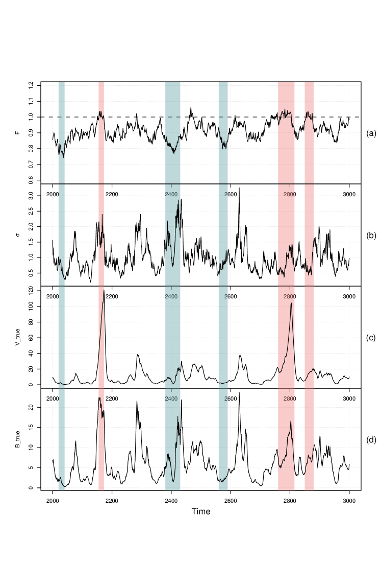
Figure 1: Typical time series of: (a) The forecast operator $F_{k}$, (b) The model error standard deviation $\sigma_{k}$, (c) The variance of the truth ${V}_{k}$, and (d) The true background error variance ${B}_{k}$ for the HBEF. The light gray (pink in the web version of the article) vertical stripes indicate events when $F_{k}>1$. The dark gray (blue in the web version of the article) vertical stripes indicate events when $|F_{k}|$ was relatively low.

4.5 Verifying the conditional Gaussianity of the state given $(x^{f},{B})$

From the equation

$${x}|x^{f},{P},{Q}\sim{\cal N}({x}^{f},B={P}+{Q}),$$ (52)

it is obvious that $x_{k}|x_{k}^{f},B_{k}$ is Gaussian if and only if so is $x_{k}-x_{k}^{f}|B_{k}$. With the true ${x}_{k}$ and ${B}_{k}$ in hand, we were able to verify if indeed ${x}_{k}-{x}^{f}_{k}\,|\,{B}_{k}\sim{\cal N}(0,{B}_{k})$. Fig.2(left) presents the respective $q$-$q$ (quantile-quantile) plots. (Note that for a Gaussian density, the $q$-$q$ plot is a straight line, with the slope proportional to the standard deviation of the empirical distribution.)

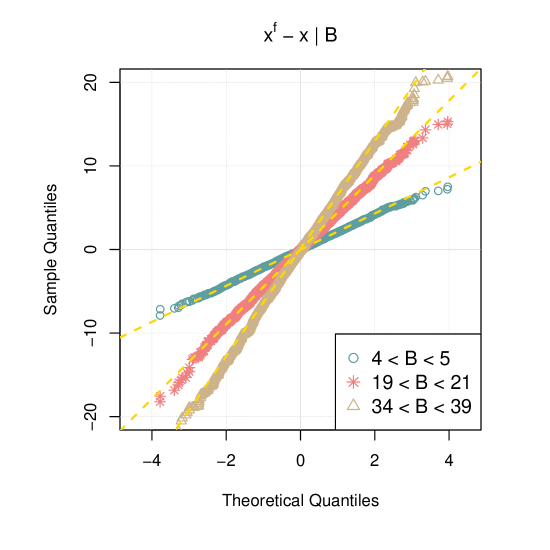
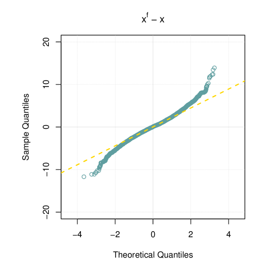
Figure 2: The Gaussian $q$-$q$ plots for the conditional pdf $p(x_{k}^{f}-x_{k}|{B}_{k})$ (left) and the unconditional pdf $p(x_{k}^{f}-x_{k})$ (right). In the left panel, the three curves correspond to the three intervals of ${B}_{k}$ indicated in the legend.

One can see that $p(x_{k}-x_{k}^{f}|{B}_{k})$ can indeed be very well approximated by a Gaussian density for low, medium, and high values of ${B}_{k}$ (the three curves in Fig.2(left)). In contrast, the unconditional density $p(x_{k}-x_{k}^{f})$ is significantly non-Gaussian with heavy tails, see Fig.2(right). So, the conditional Gaussianity of the state’s prior distribution is confirmed in our numerical experiments.

4.6 The forecast ensemble members are not drawn from the same distribution as the truth

Here, we explore the actual probability distribution of the forecast ensemble members at any given time $k$. We demonstrate that for both the EnKF and the HBEF, the variance of this distribution is often substantially biased with respect to the respective true error variance.

We start by stating that in a single data assimilation run, we cannot find out from which (continuous) probability distribution the forecast ensemble members at time $k$ are drawn (because the ensemble size is small, see assumption 1). But, following section 4.3, for each filter, we had at our disposal a number of assimilation runs that share the sequence of ${B}_{k}$. Then, if in each assimilation run, the forecast ensemble members were drawn from the distribution with the variance ${B}_{k}$ (the “null hypothesis”), we would have ${\mathsf{E}\,}S_{k}={B}_{k}$, where $S_{k}$ is the ensemble (sample) variance and the expectation is over the population of independent assimilation runs. To check if this latter equality actually holds, we estimated ${\mathsf{E}\,}S_{k}$ as the sample mean $\langle S_{k}\rangle$ for each $k$ separately using the sample of $L$ assimilation runs.

The resulting time series of the biases $\langle S_{k}\rangle-{B}_{k}$ for the EnKF and the HBEF are displayed in Fig.3 (the two lower curves) along with their respective 95% bootstrap confidence intervals. The true error variances themselves ${B}_{k}$ are also shown in Fig.3 (the two upper curves) to give an impression of the relative magnitude of the biases in $\langle S_{k}\rangle$.

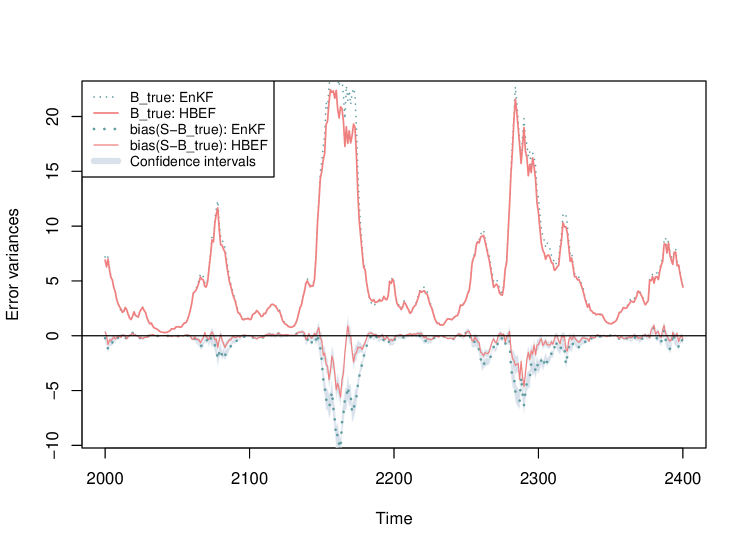
Figure 3: The two lower curves: biases in the forecast ensemble variances (with the 95% confidence intervals) for the EnKF and the HBEF. The two upper curves: the respective true error variances ${B}_{k}$.

One can see that that the biases in the ensemble variances were significantly non-zero when the true $B_{k}$ were relatively large. For the EnKF, the deviation of $\langle S_{k}\rangle$ from ${B}_{k}$ sometimes reached 50% of ${B}_{k}$. For the HBEF, the biases were less but still significant. In the small forecast error regimes, the biases became insignificant. It is also interesting to notice that the large biases were mostly negative implying that the filters were under-dispersive (despite the tuned variance inflation in the EnKF). Over a longer time window of $10^{4}$ time steps, the confidence interval did not contain zero (i.e. the bias was significantly non-zero) 78% of time for the EnKF and 62% of time for the HBEF.

Thus, we have to reject the null hypothesis and admit that forecast ensemble members are often taken from a distribution which is significantly different from the true one. This has two implications. First, the uncertainty in the sample covariances is not only due to the sampling noise but also due to an accumulated in time systematic error component. Second, the biases in the sample covariances warrant the introduction of the actual predictability ensemble covariance matrix $\boldsymbol{\Pi}_{k}$ that differs from the true covariance matrix ${\bf P}_{k}$ (see section 3.5).

The above results are worth comparing with those of Bishop and Satterfield [3], who found insignificant biases in the ensemble variances, see their Fig.2. One dissimilarity between their and our experiments was that an ensemble transform version of the EnKF was used in [3]. We employed the ensemble transform technique for both the EnKF and the HBEF and found that this led to some improvements but did not remove the biases in $S_{k}$ (not shown). A plausible reason for the difference in the conclusions is that the system in [3] was much better observed than ours (they used $R$ which was much less than the mean $V_{k}$, whereas in our study $R$ was several times larger than the mean $V_{k}$).

4.7 Verifying the primary filters

Here, we examine the accuracy of the state estimates for the HBEF and the other filters (the Var, the EnKF, and the HEnKF). In the below figures, we display their analysis RMSEs with the reference-KF analysis RMSEs subtracted.

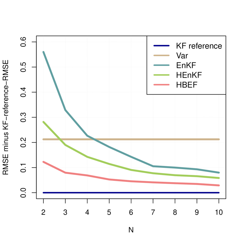
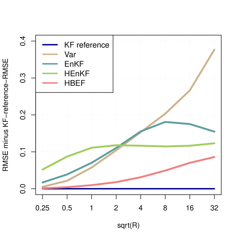
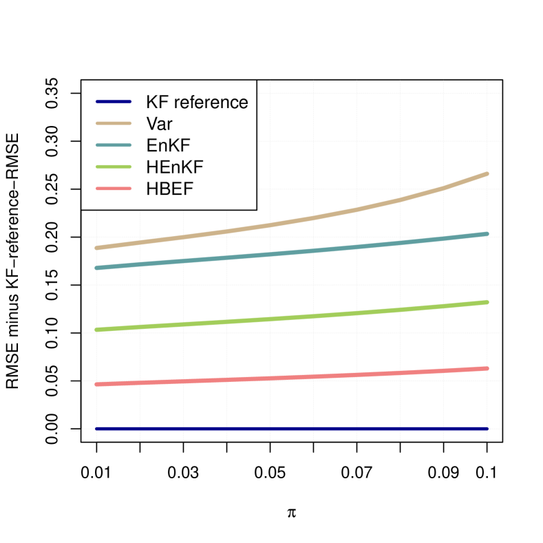
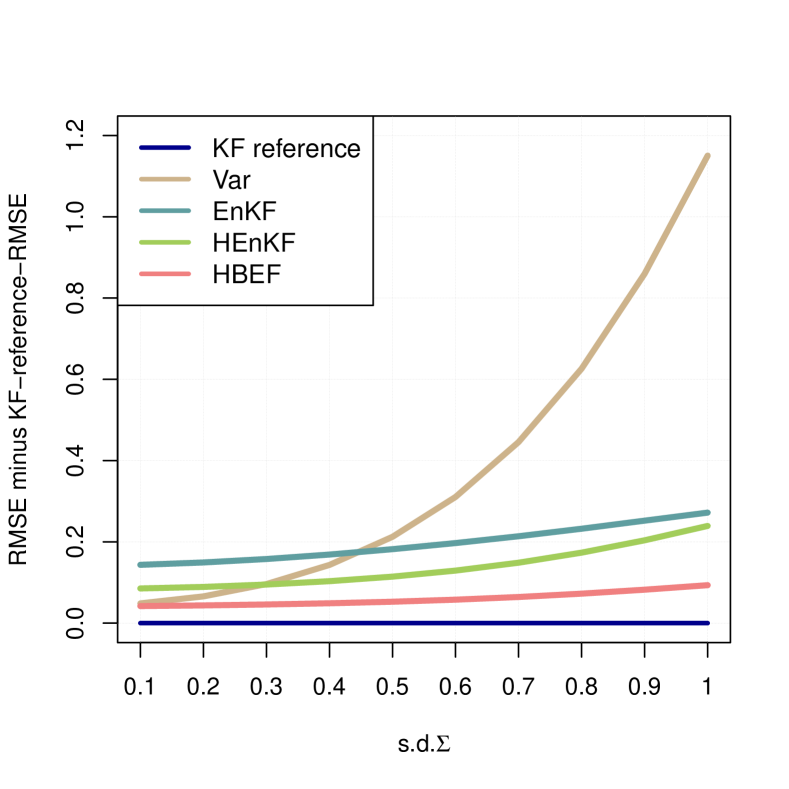
Figure 4: The filters’ analysis RMSEs of the state (with the reference-KF analysis RMSE subtracted) as functions of the ensemble size $N$ (top, left), the observation error standard deviation $\sqrt{R}$ (top, right), the degree of the system’s intermittent instability $\pi$ (bottom, left), the variability in the model error standard deviation ${\mathsf{s.d.}}\,\Sigma$ (bottom, right).

Figure 4(top, left) shows the RMSEs as functions of the ensemble size $N$. One can see that the HBEF was by far the best filter. For small $N<3$, the Var became more competitive than the EnKF and the HEnKF, but still worse than the HBEF.

Figure 4(top, right) shows the RMSEs as functions of $\sqrt{R}$. Again, the HBEF performed the best. Its relative superiority was especially substantial for the smaller values of $\sqrt{R}$. This can be explained by the prevalence of $Q$ (which is more rigorously treated in the HBEF) over $P$ (which is only sub-optimally treated in the HBEF) in this regime.

Figure 4(bottom, left) shows the RMSEs as functions of $\pi={\mathsf{P}\,}(|F_{k}|>1)$. One can see that the HBEF was uniformly and significantly better than the other filters. Note that all the filters gradually deteriorate w.r.t. the reference KF as the system becomes less stable (i.e. as $\pi$ grows), which is meaningful because errors grow faster in a less stable system.

Figure 4(bottom, right) displays the RMSEs as functions of the degree of intermittency in the model error variance quantified by ${\mathsf{s.d.}}\,\Sigma$. We see that the HBEF was still uniformly and substantially better than the EnKF and the HEnKF. For the smallest values of ${\mathsf{s.d.}}\,\Sigma$, the Var became superior to the EnKF and the HEnKF and only slightly worse than the HBEF. The fact that the Var worked relatively better for the small ${\mathsf{s.d.}}\,\Sigma$ can be explained by noting that in this regime, when the variability in $Q$ was low, the forecast error statistics were less variable and so the constant Var’s $\bar{B}$ was relatively more suitable.

Thus, in terms of the analysis RMSEs, the HBEF demonstrated its overall superiority over the competing EnKF, HEnKF, and Var filters.

4.8 Verifying the secondary filters

Recall that the HBEF’s secondary sub-filter produces the posterior estimate ${B}^{a}_{k}={P}^{a}_{k}+{Q}^{a}_{k}$ of its true forecast error variance ${B}_{k}$. The HEnKF yields its ${B}^{a}_{k}$ as described in item (iii) in section 2.7.1. The Var uses the constant $\bar{B}$ as an estimate of ${B}_{k}$, so we associate $\bar{B}$ with its ${B}_{k}^{a}$. Similarly, we identify the EnKF’s inflated ensemble variance ${S}_{k}$ with its ${B}^{a}_{k}$.

In this section, we examine the errors ${B}^{a}_{k}-B_{k}$, with the filter specific ${B}_{k}$ assessed following section 4.3. Having the true $B_{k}$ for each filter, we computed the RMSE in its $B^{a}_{k}$ estimates using averaging over the $L$ independent assimilation runs as $\Delta_{k}=\sqrt{\langle({B}^{a}_{k}-{B}_{k})^{2}\rangle}$. The resulting $\Delta_{k}$ for the HBEF and the EnKF are depicted in Fig.5, where the almost uniform and substantial superiority of the HBEF is evident.

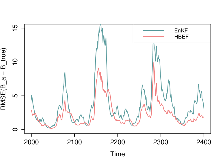
Figure 5: RMSEs in $B^{a}_{k}$ produced by the EnKF and the HBEF.

Having square averaged $\Delta_{k}$ over time, we obtained the time mean RMSEs in ${B}^{a}_{k}$. In a similar way we computed the biases in ${B}^{a}_{k}$. The results of an experiment with $10^{4}$ time steps are collected in Table 1, where it is seen that the HBEF was much more accurate in estimating its ${B}_{k}$ than the Var, the EnKF, and the HEnKF in estimating their respective true forecast error variances.

Table 1: Accuracy of the filters’ estimates of their own forecast error variance $B_{k}$

Filter	Error bias	RMSE	Mean true $B$
	${\mathsf{mean}}\,({{B}^{a}_{k}-{B}_{k}})$	${\mathsf{rms}}\,({B}^{a}_{k}-{B}_{k})$	${\mathsf{mean}}\,({{B}_{k}})$
Var	-0.9	6.5	7.6
EnKF	-1.4	6.2	7.5
HEnKF	-1.8	4.4	7.2
HBEF	-0.5	3.2	7.0

4.9 Role of feedback from observations to forecast error covariances

The HBEF with the Monte Carlo based analysis (section 3.8.2) provides an optimized way to utilize observations in updating $P$ and $Q$. In the default setup, this capability did not lead to any improvement in the performance scores (not shown), but it became significant when the filter’s model error variance was misspecified.

Specifically, we let all the filters (including the KF) “assume” that the model error variance $Q_{k}$ equals the true one multiplied by the distortion coefficient $q_{distort}$. For several values of ${q_{distort}}$ in the range from $1/16$ to $16$, we computed the RMSEs of the analyses of the state for all filters and plotted the results in Fig.6. In the HBEF with the Monte Carlo based analysis, the size of the Monte Carlo sample was $M=100$, see Eqs.(41)–(42).

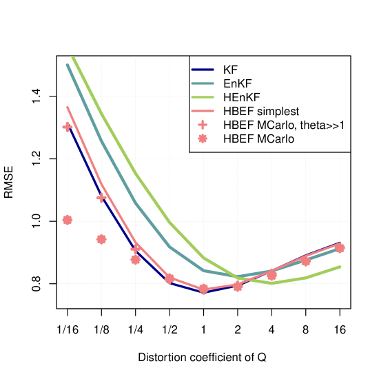
Figure 6: Analysis RMSEs of the state for the filters which used the wrong $Q$. The latter was specified to be the true $Q$ multiplied by the distortion coefficient $q_{distort}$.

To make the effect more pronounced, the observation error standard deviation was reduced to $\sqrt{R}=1$.

From Fig.6 one can see that the overall performance of the HBEF with the Monte Carlo based analysis was better than the performances of the other filters, including, we emphasize, the (now, inexact) KF. The observations-to-covariances feedback present in the Monte Carlo based HBEF (and absent in the other filters) appeared especially useful for $q_{distort}<1$. The improvement was bigger for $q_{distort}<1$ than for $q_{distort}>1$ because an underestimation of the forecast error covariances is potentially more problematic for any filter. Indeed, the overconfidence in the forecast leads to an underuse of observations and in extreme cases can even lead to filter divergence. This is why the settings with $q_{distort}<1$ left more room for improvement, particularly due to the feedback from observations to the covariances.

Another interesting conclusion can be drawn from comparing the Monte Carlo based version of the HBEF with the optimally tuned parameter $\theta$ (asterisks in Fig.6) and the same version of the HBEF but with $\theta=\infty$ (crosses). Recall that $\theta$ controls the difference between the variance $\Pi$ of the distribution of the predictability ensemble members and the true variance $P$. In the setting with $\theta=\infty$, the HBEF “assumes” that $\Pi=P$. Figure 6 clearly shows that it was indeed beneficial to get away from the traditional assumption $\Pi=P$. This again justifies our suggestion (see section 3.5) to allow the ensemble distribution to be different from the true one.

5 Discussion

5.1 Comparison with other approaches

The HBEF has two immediate predecessors, the HEnKF [28] and the EnKF-N [4, 6]. The HBEF differs from the HEnKF in the following aspects. First, in the HBEF we treat ${\bf Q}$ and ${\bf P}$ separately instead of using the total background error covariance matrix ${\bf B}$. Second, the HBEF’s forecast step is based on the persistence forecasts for the posterior point estimates of ${\bf Q}$ and ${\bf P}$ instead of that for the analysis error covariance matrix. These two improvements have led to the substantially better performance of the HBEF as compared to the HEnKF. Another difference from the HEnKF is that the Monte Carlo based HBEF permits observations to influence ${\bf Q}$ and ${\bf P}$. Experimentally, this latter feature appeared to be beneficial only when ${\bf Q}$ was significantly misspecified, though.

As compared to the EnKF-N, which integrates ${\bf B}$ out of the prior distribution, the HBEF explicitly updates the covariance matrices. This introduces memory in the covariances, which, as we have seen in the numerical experiments, can be beneficial.

In contrast to both the HEnKF and the EnKF-N, the HBEF in its present formulation does not treat the uncertainty in the prior mean state vector (this may be worth exploring in the future). But the HBEF systematically treats the uncertainty in ${\bf Q}$, which was assumed to be known in [28] and equal to zero in [4, 5, 6].

5.2 Restrictions of the proposed technique

First, the HBEF heavily relies on the conditional Gaussian prior distribution of the state. It is this assumption that greatly simplifies the analysis algorithm, but in a nonlinear context, it becomes an approximation, whose validity is to be verified.

Second, the HBEF makes use of the inverse Wishart prior distribution for the covariance matrices. There is no justification for this hypothesis other than partial analytical tractability of the resulting analysis equations, so other choices can be explored.

5.3 Practical applications

In order to apply the proposed technique to real-world high-dimensional problems, simplifications are needed because the $n\times n$ covariance matrices will be too large to be stored and handled. The computational burden can be reduced in different ways. Here is one of them. First, let the covariances to be defined on a coarse grid. Second, localize (taper) the covariances and store only non-zero covariance matrix entries. Third, use the simplest version of the HBEF.

Another possibility is to fit a parametric covariance model to current covariances and impose persistence for the parameters of the model. In this case, the simplest version of the HBEF would become close to practical ensemble variational schemes, but with climatological covariances replaced by evolving recent-past-data based covariances.

In high dimensions, the persistence forecast for the covariances seems to be worth improving. Specifically, one may wish to somehow spatially smooth ${\bf P}^{a}_{k-1}$ and ${\bf Q}^{a}_{k-1}$ in Eq.(47)—because it is meaningful that smaller scales in ${\bf P}^{a}_{k-1}$ and ${\bf Q}^{a}_{k-1}$ have less chance to survive until the next assimilation cycle than larger scales. Another way to improve the empirical forecast of the covariance matrices is to introduce a kind of “regression to the mean” making use of the time mean covariances. This would imply that the HBEF would cover not only EnKF but also ensemble variational hybrids as a special case.

The ultimate goal with the HBEF will be to obtain effective covariance regularization as a by-product of the hierarchical analysis scheme without using any ad-hoc device (as it was proposed for the EnKF-N in [4] and partially tested in [6]).

6 Conclusions

The progress made in this study can be summarized as follows.

• We have acknowledged that in most applications, the EnKF works with: (i) the explicitly unknown and variable model error covariance matrix ${\bf Q}_{k}$, (ii) the partially known (through ensemble covariances) background error covariance matrix. Under these explicit restrictions, we have proposed a new Hierarchical Bayes Ensemble Filter (HBEF) that optimizes the use of observational and ensemble data by treating ${\bf Q}_{k}$ and the predictability covariance matrix ${\bf P}_{k}$ as random matrices to be estimated in the analysis along with the state. The ensemble members are treated in the HBEF as generalized observations on the covariance matrices.

• With the new HBEF filter, in the course of filtering, the prior and posterior distributions of the state remain conditionally (given ${\bf P}_{k},{\bf Q}_{k}$) Gaussian provided that: (i) it is so at the start of the filtering, (ii) observation errors are Gaussian, (iii) the dynamics and the observation operators are linear, and (iv) model errors are conditionally Gaussian given ${\bf Q}_{k}$. Unconditionally, the prior and posterior distributions of the state are non-Gaussian.

• The HBEF is tested with a new one-variable doubly stochastic model of truth. The model has the advantage of providing the means to assess the instantaneous variance of the truth and the true filter’s error variances. The HBEF is found superior the EnKF and the HEnKF [28] under most regimes of the system, most data assimilation setups, and in terms of performance of both primary and secondary filters.

• The availability of the true error variances has permitted us to experimentally prove that the forecast ensemble variances in both the EnKF and the HBEF are often significantly biased with respect to the true variances.

• It is shown that the HBEF’s feedback from observations to the covariances can be beneficial.

• The simplest version of the HBEF is designed to be affordable for practical high-dimensional applications on existing computers.

7 Acknowledgments

The authors are very grateful to the two anonymous reviewers, whose valuable comments helped to significantly improve the manuscript.

References

Appendix A Inverse Wishart distribution

In Bayesian statistics, the inverse Wishart distribution (e.g. [20, 1, 19]) is the standard choice for the prior distribution of a random covariance matrix, because inverse Wishart is the so-called conjugate distribution for the Gaussian likelihood, e.g. [1, 19]. The inverse Wishart pdf is defined for symmetric matrices and is non-zero for positive definite ones:

$$p({\bf Z})\propto\frac{1}{|{\bf Z}|^{\frac{\nu+n+1}{2}}}\rm e^{-\frac{1}{2}\operatorname{tr}({\bf Z}^{-1}{\boldsymbol{\Sigma}})},$$ (53)

where $\nu>n+1$ is the so-called number of degrees of freedom (which controls the spread of the distribution: the greater $\nu$, the less the spread) and ${\boldsymbol{\Sigma}}$ is the positive definite scaling matrix. Using the mean value ${\bf\bar{Z}}={\mathsf{E}\,}{\bf Z}={\boldsymbol{\Sigma}}/(\nu-n-1)$ instead of the scaling matrix allows us to reparametrize Eq.(53) as

$$p({\bf Z})=p({\bf Z}|\theta,{\bf\bar{Z}})\propto\frac{1}{|{\bf Z}|^{\frac{\theta}{2}+n+1}}\rm e^{-\frac{\theta}{2}\operatorname{tr}({\bf Z}^{-1}{\bf\bar{Z}})},$$ (54)

where we have introduced a new scale parameter $\theta=\nu-n-1>0$, which we call the sharpness parameter (the higher $\theta$, the narrower the density). We symbolically write Eq.(54) as

$${\bf Z}\sim{\cal IW}(\theta,{\bf\bar{Z}}).$$ (55)

We prefer our parametrization $(\theta,{\bf\bar{Z}})$ to the common one $(\nu,\boldsymbol{\Sigma})$ because ${\bf\bar{Z}}$ has the clear meaning of the (important) mean ${\bf Z}$ matrix. Summarizing, the inverse Wishart pdf has two parameters: the sharpness parameter $\theta$ (a scalar) and the mean ${\bf\bar{Z}}$ (a positive definite matrix).

Appendix B Assimilation of conditionally Gaussian generalized observations in an update of their covariance matrix

Here, we outline, following e.g. [19], the procedure of assimilation of independent draws from the distribution ${\cal N}({\bf m,Z})$, where ${\bf m}$ is the known vector and ${\bf Z}$ the unknown random symmetric positive definite matrix, whose prior distribution is inverse Wishart with the density specified by Eq.(54).

Let us take a draw ${\bf x}^{e}(i)|{\bf Z}\sim{\cal N}({\bf m,Z})$, which we interpret as a member of an ensemble. Then, obviously,

$$p({\bf x}^{e}(i)|{\bf Z})\propto\frac{1}{|{\bf Z}|^{\frac{1}{2}}}\rm e^{-\frac{1}{2}({\bf x}^{e}(i)-{\bf m})^{\top}{\bf Z}^{-1}({\bf x}^{e}(i)-{\bf m})}.$$ (56)

We stress that Eq.(56) is nothing other than the likelihood of ${\bf Z}$ given the ensemble member ${\bf x}^{e}(i)$. Further, having the ensemble ${\bf X}^{e}=({\bf x}^{e}(1),\dots,{\bf x}^{e}(N))$ of $N$ independent members all taken from ${\cal N}({\bf m,Z})$, we can write down the respective ensemble likelihood as the product of the partial likelihoods:

$$p({\bf X}^{e}|{\bf Z})\propto\frac{1}{|{\bf Z}|^{\frac{N}{2}}}\rm e^{-\frac{1}{2}\sum_{i=1}^{N}({\bf x}^{e}(i)-{\bf m})^{\top}{\bf Z}^{-1}({\bf x}^{e}(i)-{\bf m})}=\frac{1}{|{\bf Z}|^{\frac{N}{2}}}\rm e^{-\frac{N}{2}\operatorname{tr}({\bf S}{\bf Z}^{-1})},$$ (57)

where

$${\bf S}=\frac{1}{N}\sum_{i=1}^{N}({\bf x}^{e}(i)-{\bf m})\,({\bf x}^{e}(i)-{\bf m})^{\top}$$ (58)

is the sample covariance matrix. But having the likelihood $p({\bf X}^{e}|{\bf Z})$ means that ${\bf X}^{e}$ (and its members ${\bf x}^{e}(i)$) can be regarded and treated as (generalized) observations on ${\bf Z}$. In particular, the ensemble can be assimilated in the standard way using the Bayes theorem. Indeed, having the prior pdf of ${\bf Z}$, Eq.(54), we obtain the posterior

$$p^{a}({\bf Z})\propto p({\bf Z}|\theta,{\bf\bar{Z}},{\bf X}^{e})\propto p({\bf Z}|\theta,{\bf\bar{Z}})\cdot p({\bf X}^{e}|{\bf Z})\propto\frac{1}{|{\bf Z}|^{\frac{\theta^{a}}{2}+n+1}}\rm e^{-\frac{\theta^{a}}{2}\operatorname{tr}({\bf Z}^{-1}{\bf Z}^{a})},$$ (59)

where

$$\theta^{a}=\theta+N\qquad\mbox{and}\qquad{\bf Z}^{a}=\frac{\theta{\bf\bar{Z}}+N{\bf S}}{\theta+N}.$$ (60)

In the right-hand side of Eq.(59), we recognize again the inverse Wishart pdf (hence its conjugacy), see Eq.(54), with $\theta^{a}$ being the posterior sharpness parameter and ${\bf Z}^{a}$ being the posterior mean of ${\bf Z}$. Consequently, ${\bf Z}^{a}$ is the mean-square optimal point estimate of ${\bf Z}$ given both the prior and ensemble information. So, we have optimally assimilated the (conditionally Gaussian) ensemble data to update the (inverse Wishart) prior distribution of the random covariance matrix.

Appendix C Integral w.r.t. a matrix

For a general $n\times n$-matrix ${\bf C}$, the integral $\int f({\bf C})\,{\rm d}{\bf C}$ of a scalar function $f({\bf C})$ over the space of all matrices with real entries is defined as follows. First, we vectorize ${\bf C}$, i.e. build the vector $\vec{\bf C}$ of length $n^{2}$ that comprises all entries of ${\bf C}$. Then, we simply identify $\int f({\bf C})\,{\rm d}{\bf C}$ with $\int f({\bf C})\,{\rm d}\vec{\bf C}$, that is, with the traditional multiple (Lebesgue or Riemann) integral over the Euclidean space of dimensionality $n^{2}$.

The integral w.r.t. a symmetric positive definite matrix is defined in a similar way. The difference from the general matrix case is that the vectorization here involves collecting in $\vec{\bf C}$ only algebraically independent matrix entries (e.g. the upper triangle of ${\bf C}$) and the multiple integral is over the set (the convex cone) of those $\vec{\bf C}$ that correspond to positive definite matrices.

Appendix D List of main symbols

$()^{a}$	posterior (analysis) pdf (i.e. conditioned on past and current data) and its parameters
$()^{f}$	prior (forecast) pdf (i.e. conditioned on past data) and its parameters
$\widetilde{(})$	sub-posterior pdf (i.e. conditioned on past data and current ensemble data) and its parameters
$()^{fe},()^{ae}$	forecast ensemble / analysis ensemble
$()^{me}$, $()^{pe}$	model error ensemble / predictability ensemble
${\bar{.}}$	time mean value
$\langle.\rangle$	average over $L$ independent realizations of the truth / assimilation runs
${\bf A}$	posterior (analysis error) covariance matrix
${\bf B}$	prior (forecast error) covariance matrices
${\bf F}$	forecast operator
${\bf H}$	observation operator
$i$	ensemble member index
${\bf K}$	Kalman gain matrix
$k$	time instance index
$L$	number of independent assimilation runs
$l({\bf B|y})$	observation likelihood of the matrix ${\bf B}$
${\bf m}^{a}$	posterior mean ${\bf x}$ given ${\bf P,Q}$
$n$	dimensionality of state space
$N$	ensemble size
$p$	probability density function (pdf)
${\bf P,Q,R}$	predictability error / model error / observation error covariance matrix
${\bf S}$	sample (ensemble) covariance matrix
${V}_{k}$	${\mathsf{Var}}\,x_{k}$
${\bf x}$	state vector, “truth”
${\bf x}^{a}$	posterior mean vector and its approximations (deterministic analysis)
${\bf x}^{f}$	prior mean vector (identified in this study with the deterministic forecast)
${\bf x}^{..}(i),{\bf x}^{e}(i)$	ensemble member
${\bf X}$	ensemble
${\bf y}$	observation vector
${\bf Y}$	observation and ensemble data combined
${\cal IW}$	inverse Wishart distribution (parametrized according to A)
${\cal N}({\bf m,B})$	Gaussian distribution with the mean ${\bf m}$ and covariance matrix ${\bf B}$
$\boldsymbol{\varepsilon}$	model error (system noise) vector
$\boldsymbol{\eta}$	observation error vector
$\theta,\phi,\chi$	sharpness parameters for the inverse Wishart pdfs
$\pi$	portion of time the process $F_{k}$ is greater than 1 in modulus
$\sigma$	(time-specific) model error standard deviation
${\mathsf{E}\,}$	expectation operator
${\mathsf{rms}}\,$, RMSE	root-mean-square value / error
${\mathsf{s.d.}}\,,{\mathsf{Var}}\,$	standard deviation / variance
$\operatorname{tr}$	matrix trace
$\propto$	proportionality
$\sim$	has (corresponds to) the probability distribution
$1:k$	concatenation from the time instance $1$ to the time instance $k$

References

- Anderson [2003] T. Anderson. An introduction to multivariate statistical analysis. Wiley Interscience, 2003.
- Berliner [1996] L. M. Berliner. Hierarchical Bayesian time series models. In Maximum entropy and Bayesian methods, pages 15–22. Springer, 1996.
- Bishop and Satterfield [2013] C. H. Bishop and E. A. Satterfield. Hidden error variance theory. Part I: Exposition and analytic model. Mon. Weather Rev., 141(5):1454–1468, 2013.
- Bocquet [2011] M. Bocquet. Ensemble Kalman filtering without the intrinsic need for inflation. Nonlin. Process. Geophys., 18(5):735–750, 2011.
- Bocquet and Sakov [2012] M. Bocquet and P. Sakov. Combining inflation-free and iterative ensemble Kalman filters for strongly nonlinear systems. Nonlin. Process. Geophys., 19(3):383–399, 2012.
- Bocquet et al. [2015] M. Bocquet, P. Raanes, and A. Hannart. Expanding the validity of the ensemble Kalman filter without the intrinsic need for inflation. Nonlin. Process. Geophys., 22(6):645–662, 2015.
- Buehner et al. [2013] M. Buehner, J. Morneau, and C. Charette. Four-dimensional ensemble-variational data assimilation for global deterministic weather prediction. Nonlin. Process. Geophys., 20(5):669–682, 2013.
- Carlin and Louis [2000] B. P. Carlin and T. A. Louis. Bayes and empirical Bayes methods for data analysis. Chapman and Hall/CRC, 2000.
- Chapelle et al. [2013] D. Chapelle, M. Fragu, V. Mallet, and P. Moireau. Fundamental principles of data assimilation underlying the Verdandi library: applications to biophysical model personalization within euHeart. Med. Biol. Eng. Comput., 51(11):1221–1233, 2013.
- Deckmyn and Berre [2005] A. Deckmyn and L. Berre. A wavelet approach to representing background error covariances in a limited area model. Mon. Weather Rev., 133(5):1279–1294, 2005.
- Dee et al. [1985] D. P. Dee, S. E. Cohn, A. Dalcher, and M. Ghil. An efficient algorithm for estimating noise covariances in distributed systems. IEEE Trans. Autom. Control, 30(11):1057–1065, 1985.
- Du and Smith [2012] H. Du and L. A. Smith. Parameter estimation through ignorance. Physical Review E, 86(1):016213, 2012.
- Eliassen [1954] A. Eliassen. Provisional report on calculation of spatial covariance and autocorrelation of the pressure field. Videnskaps-Akademiets Institutt for Vaer-og Klimaforskning, Oslo, Norway, Report No.5, pages 1–11, 1954.
- Evensen [1994] G. Evensen. Sequential data assimilation with a nonlinear quasi-geostrophic model using Monte Carlo methods to forecast error statistics. J. Geophys. Res., 99(10):10,143–10,162, 1994.
- Fisher [2003] M. Fisher. Background error covariance modelling. Proc. ECMWF Semin. on recent developments in data assimilation for atmosphere and ocean, 8-12 September 2003, pages 45–64, 2003.
- Fournier et al. [2010] A. Fournier, G. Hulot, D. Jault, W. Kuang, A. Tangborn, N. Gillet, E. Canet, J. Aubert, and F. Lhuillier. An introduction to data assimilation and predictability in geomagnetism. Space Sci. Rev., 155(1-4):247–291, 2010.
- Furrer and Bengtsson [2007] R. Furrer and T. Bengtsson. Estimation of high-dimensional prior and posterior covariance matrices in Kalman filter variants. J. Multivar. Anal., 98(2):227–255, 2007.
- Gandin [1965] L. Gandin. Objective Analysis of Meteorological Fields. Gidrometizdat, Leningrad, 1963. Translated from Russian into English by the Israel Program for Scientific Translations, Jerusalem, 1965.
- Gelman et al. [2004] A. Gelman, J. Carlin, H. Stern, and D. Rubin. Bayesian data analysis. Chapman and Hall/CRC, 2004.
- Gupta and Nagar [1999] A. K. Gupta and D. K. Nagar. Matrix variate distributions. CRC Press, 1999.
- Houtekamer and Mitchell [2001] P. L. Houtekamer and H. Mitchell. A sequential ensemble Kalman filter for atmospheric data assimilation. Mon. Weather Rev., 129(1):123–137, 2001.
- Kroese et al. [2011] D. Kroese, T. Taimre, and Z. Botev. Handbook of Monte Carlo methods. Wiley, 2011.
- Lahoz et al. [2010] W. Lahoz, B. Khattatov, and R. Menard. Data assimilation. Springer, 2010.
- Le and Zidek [2006] N. D. Le and J. V. Zidek. Statistical analysis of environmental space-time processes. Springer, 2006.
- Ledoit and Wolf [2004] O. Ledoit and M. Wolf. A well-conditioned estimator for large-dimensional covariance matrices. J. Multivar. Anal., 88(2):365–411, 2004.
- Lorenc et al. [2014] A. C. Lorenc, N. E. Bowler, A. M. Clayton, S. R. Pring, and D. Fairbairn. Comparison of hybrid-4DEnVar and hybrid-4DVar data assimilation methods for global NWP. Mon. Weather Rev., 143(2015):212–229, 2014.
- Lorenz [1963] E. N. Lorenz. Deterministic nonperiodic flow. J. Atmos. Sci., 20(2):130–141, 1963.
- Myrseth and Omre [2010] I. Myrseth and H. Omre. Hierarchical ensemble Kalman filter. SPE Journal, 15(2):569–580, 2010.
- Niu et al. [2014] S. Niu, Y. Luo, M. C. Dietze, T. F. Keenan, Z. Shi, J. Li, and F. S. C. III. The role of data assimilation in predictive ecology. Ecosphere, 5(5):art65, 2014.
- Oliver et al. [2011] D. Oliver, Y. Zhang, H. Phale, and Y. Chen. Distributed parameter and state estimation in petroleum reservoirs. Comput. and Fluids, 46(12):70–77, 2011.
- Purser and Wu [2003] R. Purser and W. Wu. Numerical aspects of the application of recursive filters to variational statistical analysis. Part I: Spatially homogeneous and isotropic Gaussian covariances. Mon. Weather Rev., 131(8):1524–1535, 2003.
- Rabier et al. [1998] F. Rabier, A. McNally, E. Andersson, P. Courtier, P. Unden, J. Eyre, A. Hollingsworth, and F. Bouttier. The ECMWF implementation of three-dimensional variational assimilation (3D-Var). II: Structure functions. Q. J. Roy. Meteorol. Soc., 124(550):1809–1829, 1998.
- Rhodes and Hollingsworth [2009] C. Rhodes and T. D. Hollingsworth. Variational data assimilation with epidemic models. J. Theor. Biol., 258(4):591–602, 2009.
- Robert [2007] C. Robert. The Bayesian choice. Springer, 2007.
- Sacher and Bartello [2008] W. Sacher and P. Bartello. Sampling errors in ensemble Kalman filtering. part I: Theory. Mon. Weather Rev., 136(8):3035–3049, 2008.
- Tippett et al. [2003] M. K. Tippett, J. L. Anderson, C. H. Bishop, T. M. Hamill, and J. S. Whitaker. Ensemble square root filters. Mon. Weather Rev., 131(7):1485–1490, 2003.
- Tjøstheim [1986] D. Tjøstheim. Some doubly stochastic time series models. J. Time Ser. Anal., 7(1):51–72, 1986.
- Trudinger et al. [2008] C. Trudinger, M. Raupach, P. Rayner, and I. Enting. Using the Kalman filter for parameter estimation in biogeochemical models. Environmetrics, 19(8):849–870, 2008.
- van Leeuwen [2009] P. J. van Leeuwen. Particle filtering in geophysical systems. Mon. Weather Rev., 137(12):4089–4114, 2009.
- Weaver and Courtier [2001] A. Weaver and P. Courtier. Correlation modelling on the sphere using a generalized diffusion equation. Q. J. Roy. Meteorol. Soc., 127(575):1815–1846, 2001.
- Yoshida et al. [2008] R. Yoshida, M. Nagasaki, R. Yamaguchi, S. Imoto, S. Miyano, and T. Higuchi. Bayesian learning of biological pathways on genomic data assimilation. Bioinformatics, 24(22):2592–2601, 2008.