Simultaneously modelling far-infrared dust emission and its relation to CO emission in star forming galaxies

Abstract

We present a method to simultaneously model the dust far-infrared spectral energy distribution (SED) and the total infrared $-$ carbon monoxide (CO) integrated intensity ($S_{\rm IR}$$-$$I_{\rm CO}$) relationship. The modelling employs a hierarchical Bayesian (HB) technique to estimate the dust surface density, temperature ($T_{\rm eff}$), and spectral index at each pixel from the observed far-infrared (FIR) maps. Additionally, given the corresponding CO map, the method simultaneously estimates the slope and intercept between the FIR and CO intensities, which are global properties of the observed source. The model accounts for correlated and uncorrelated uncertainties, such as those present in Herschel observations. Using synthetic datasets, we demonstrate the accuracy of the HB method, and contrast the results with common non-hierarchical fitting methods. As an initial application, we model the dust and gas on 100 pc scales in the Magellanic Clouds from Herschel FIR and NANTEN CO observations. The slopes of the log$S_{\rm IR}$$-$log$I_{\rm CO}$ relationship are similar in both galaxies, falling in the range 1.1$-$1.7. However, in the SMC the intercept is nearly 3 times higher, which can be explained by its lower metallicity than the LMC, resulting in a larger $S_{\rm IR}$ per unit $I_{\rm CO}$. The HB modelling evidences an increase in $T_{\rm eff}$ in regions with the highest $I_{\rm CO}$ in the LMC. This may be due to enhanced dust heating in the densest molecular regions from young stars. Such simultaneous dust and gas modelling may reveal variations in the properties of the ISM and its association with other galactic characteristics, such as star formation rates and/or metallicities.

1 Introduction

Understanding the formation of planets, stars, and the dynamics of the host galaxies, including galaxy clusters, invariably requires a thorough assessment of the physical conditions of the interstellar medium (ISM). Targeted surveys employing ground and space based telescopes have provided a wealth of multi-wavelength data, enabling the concurrent study of various facets of the ISM. For instance, infrared (IR) and sub-millimeter observations from Spitzer (Werner et al., 2004), Herschel (Pilbratt et al., 2010), CARMA, NANTEN (and other ground based observatories), have revealed the properties of dust and gas prevalent in the ISM, such as the temperature, chemical composition, and density. Flexible statistical methods and well tested theoretical models are necessary to accurately estimate such properties, as well as identify unanticipated features in the large and diverse observational datasets.

The spectral energy distribution (SED) of dust can reveal its physical characteristics. Dust grains absorb stellar radiation, and releases this heat in the form of far infrared (FIR) emission. Observed FIR intensities appear to follow a power-law modified blackbody (Hildebrand, 1983). Dust properties such as the temperature and emissivity control the shape of the emergent FIR SED. Therefore, accurately constraining the SED parameters from IR observations provides information about the physical characteristics of dust. However, modelling the SED is not trivial, as there are significant degeneracies between the parameters. Notably, when fitting SEDs without careful consideration of noise and the underlying correlation between physical properties, the degeneracy between the dust temperature and spectral index leads to an artificial anti-correlation between the estimated parameters (e.g. Blain et al., 2003; Schnee et al., 2007; Shetty et al., 2009b; Juvela & Ysard, 2012). Hierarchical statistical methods can rigorously account for degeneracies and measurement uncertainties, thereby providing accurate SED parameter estimates (e.g. Kelly et al., 2012).

On large spatial scales ( $\buildrel>\over{\sim}$ 50 $-$ 100 pc), FIR emission traces warm dust heated by the stars. Emission from colder dust (with temperatures  $\buildrel<\over{\sim}$ 20 K) will pale in comparison, as the FIR intensity rises strongly with temperature. All inferred dust parameters, such as the temperatures and column densities, must be consistent with other constraints, including the relationship between the dust and gas, and/or the nature of stellar radiation. Hierarchical models are well-suited for such analyses, as they naturally allow for the simultaneous parameter estimates of diverse ISM components from multi-wavelength datasets. Such simultaneous modelling could potentially further reveal the association, or lack thereof, of the dust and the stellar component.

The molecular ISM is considered to be the direct precursor to the formation of stars, since most young stars are predicted and observed to be embedded in molecular gas (see Mac Low & Klessen, 2004; McKee & Ostriker, 1977; Fukui & Kawamura, 2010, and references therein). The lowest rotational transitions of carbon monoxide (CO) are frequently utilized as tracers of molecular gas. In particular, the $J=1-0$ transition is easily excited at typical densities ($n\approx 100$ cm^-3) and temperatures (10 $-$ 100 K) of molecular clouds, and emits at frequencies ($\approx$ 115 GHz) easily detected with ground based sub-mm telescopes. It is therefore one of the most widely employed tracers of the star-forming ISM.

Given the formation of stars in the molecular ISM traced by CO, and dust heating from young stars, there is an expectation for some correlation between the CO and FIR intensities. Schmidt (1959) predicted that the rate of star formation ($\Sigma_{\rm SFR}$) should be governed by the amount of gas through a power-law scaling. Kennicutt (1989, 1998) indeed found a tight relationship between $\Sigma_{\rm SFR}$ and the molecular gas surface density ($\Sigma_{\rm mol}$) when integrating over whole galaxies. More recently, resolved observations have also revealed an increasing trend of $\Sigma_{\rm SFR}$ with $\Sigma_{\rm mol}$ (e.g. Bigiel et al., 2008; Leroy et al., 2012). However, the indices of the power-law relationship appear to vary between normal galaxies (e.g. Bigiel et al., 2008; Shetty et al., 2013), with most galaxies appearing to favor a sub-linear relationship (Shetty et al., 2013, 2014b). Many of these studies rely on either on monochromatic IR$-$$\Sigma_{\rm SFR}$ tracers, such as 24 µm, or a second tracer to account for the un-absorbed stellar radiation, such as UV or H$\alpha$. In normal and starbursting galaxies, dust absorbs nearly all UV radiation, and so its total IR emission is employed as a proxy for the star formation rate, though there can be significant uncertainties in such conversions (e.g. Dale et al., 2005; Pope et al., 2006). Dust radiative heating from young stars is expected to decrease in low metallicity systems (Calzetti et al., 2007), requiring alternative conversion factors compared to normal or starbursting galaxies (see review by Kennicutt & Evans, 2012). Indeed, questions remain on the relationship between the CO brightness and any star formation tracer such as the dust luminosity, including the possible effects of other galaxy properties, such as Hubble type, metallicity, and/or stellar mass.

Accurately estimating any relationship between the emission from gas and dust requires sound statistical methods. For example, linear regression is commonly employed for estimating the slope of the gas $-$ SFR relationship. Some linear regression techniques are known to produce inaccurate parameter estimates. For instance, when measurement uncertainties in the predictor is ignored, the best-fit slope will be biased towards zero (Akritas & Bershady, 1996). Additionally, when the dataset consists of repeated measures from a number of individuals, fitting a single line to the pooled data conceals variations in the parameters between individual members within the population. Hierarchical statistical methods can naturally account for both of these issues, and have been shown to provide accurate parameter estimates for both linear and non-linear models including measurement uncertainties (e.g. Carroll et al., 2006; Gelman et al., 2004; Kelly, 2007).

In this work, we develop a hierarchical Bayesian method to assess the relationship between the CO and total FIR intensities. The method simultaneously estimates the parameters of the dust SED at each position, as well as the global underlying CO $-$ total FIR relationship. Such a hierarchical method estimates the spatial variation in dust properties, while self-consistently measuring the large scale relationship between dust and gas. Consequently, the resulting parameter estimates and their distributions probe for any inconsistencies between the observational data and the model SED and CO $-$ FIR relationship. Furthermore, measurement uncertainties are naturally propagated throughout the analysis, leading to final parameter estimates that robustly accounts for observational noise.

As a first application, we apply the method to Herschel FIR and NANTEN CO observations of the Large and Small Magellanic Clouds (LMC and SMC). Due to their proximity (50 - 60 kpc), these galaxies allow for detailed studies of their ISM. The Magellanic Clouds have metallicities that are lower than the Milky Way, 0.2 Z_⊙ for the SMC and 0.5 Z_⊙ in the LMC (Russell & Dopita, 1992). The factor of $\sim$2 variation in metallicities between the Magellanic Clouds may cause detectable differences in their dust and gas properties. From the HERITAGE survey data (Meixner et al., 2013), Roman-Duval et al. (2014) found significant differences in the dust-to-gas ratios between the two galaxies. Given their large angular size, the Magellanic Clouds present the opportunity to test the effect of averaging over large regions, and compare any derived trends with the small scale properties of the ISM. Here, as an initial application of the hierarchical Bayesian method, we model the SED of the Magellanic Clouds on large 100 pc scales with single modified blackbodies, in conjunction with CO maps to quantify the CO $-$ FIR relationship.

This paper is organized as follows. In the next section, we present the equations governing the assumed CO $-$ FIR relationship, and the model dust SED. We also provide a description of hierarchical Bayesian methods before displaying the full hierarchical model. In Section 3 we demonstrate the accuracy of the model on two synthetic datasets. For comparison, we also present results using common non-hierarchical fitting methods. In the subsequent section, we apply the hierarchical Bayesian method to observational data of the Magellanic Clouds. We interpret and discuss the results in the context of previous results in Section 5, and summarize the method and our findings in Section 6.

2 Modelling Method

We explore the relationship between gas and dust throughout a galaxy by characterizing the relationship between CO and FIR emission across the projected face of the galaxy, treating the lines of sight corresponding to pixels as probing regions that independently sample a global, stochastic CO–FIR relationship. A more sophisticated treatment would additionally model spatial correlation and dependence. Our focus here is to develop and implement a framework that can correctly account for pixel-specific variability (from measurement error). Our hierarchical framework can be generalized to account for spatial dependence, but we leave that for future work.

2.1 Underlying relationships

Thermal emission from dust grains is usually modelled with a power-law modified Plank spectrum. The observed surface brightness $S_{\nu}$ at a given frequency $\nu$ is:

$$S_{\rm\nu}=\Sigma_{\rm d}B_{\rm\nu}(T_{\rm eff})\kappa_{0}(\nu/\nu_{0})^{\beta_{\rm eff}}$$ (1)

where $\Sigma_{\rm d}$ is the dust surface density, $T_{\rm eff}$ is the dust temperature, and $\kappa_{\nu}=\kappa_{0}(\nu/\nu_{0})^{\beta_{\rm eff}}$ is the frequency dependent dust opacity, which depends on the spectral index $\beta_{\rm eff}$. The SED of a pure blackbody follows the Planck function:

$$B_{\rm\nu}(T_{\rm eff})=\frac{2h\nu^{3}/c^{2}}{\exp(h\nu/k_{B}T_{\rm eff})-1}$$ (2)

where $h$, $c$, and $k_{B}$ are the Planck constant, speed of light, and Boltzmann constant, respectively.

Equation (1) is a simplified model of any emergent SED, as it employs a number of approximations about the dust along the line of sight (LoS). As dust absorbs the radiation from young stars, the dust temperature depends on the distances to the these stars. Consequently, a single $T_{\rm eff}$ does not accurately model the emergent SED. The estimated temperature may better reflect a luminosity weighted temperature, and is an upper limit to the coldest temperature along the LoS (e.g. Shetty et al., 2009b; Malinen et al., 2011; Juvela & Ysard, 2012). Similarly, dust grains along the LoS can vary in composition or size and may have a range of spectral indices. Accordingly, we will only consider the estimated temperature and spectral index to be adequate approximations for describing the shape of the emergent SED. Following the convention of Gordon et al. (2014), we will therefore refer to these quantities as the “effective” temperature or spectral index (hence the subscript on $T_{\rm eff}$ and $\beta_{\rm eff}$).

The total FIR intensity $S_{\rm IR}$ can be computed by integrating the SED over all frequencies:

$$S_{\rm IR}=\int S_{\rm\nu}d\nu=\Sigma_{\rm d}\int B_{\rm\nu}(T_{\rm eff})\kappa_{\nu}d\nu$$ (3)

We model the relationship between the CO intensity $I_{\rm CO}$ and $S_{\rm IR}$ through a power-law, which translates to a linear trend in log-space:

$$\log(S_{\rm IR}/S_{\rm fid})=A+n\log(I_{\rm CO}/I_{\rm fid})$$ (4)

where $S_{\rm fid}=1\,{\rm MJy\,Hz\,sr}^{-1}$ and $I_{\rm fid}=1\,{\rm K\,km\,s}^{-1}$ are fiducial values to make the arguments of the logarithms dimensionless. Note that when CO is assumed to be a linear tracer of molecular gas, $I_{\rm CO}$ will be proportional to $\Sigma_{\rm mol}$. A common assumption for normal star-forming galaxies is that dust is mostly heated by newly born stars, so that dust thermal emission indirectly traces the amount of star formation. Since the amount of dust heating depends on metallicity, among other ISM properties, the FIR $-$ SFR relationship may vary with environment. We choose not to employ any conversion factor, and only focus on estimating the total FIR $-$ CO relationship. Note that if there were any constant FIR $-$ SFR scaling, the slope in equation (4) is the exponent in the Kennicutt-Schmidt (KS) relationship:

$$\Sigma_{\rm SFR}=a\Sigma_{\rm mol}^{n}.$$ (5)

For given values of $A$ and $n$, the observed CO map and equation (4) set $S_{\rm IR}$ at each location. Combined with the dust SED model in equations (1) $-$ (3), the dust surface density is constrained:

$$\log\Sigma_{\rm d}=\log S_{\rm IR}-\log\left(\int B_{\rm\nu}(T_{\rm eff})\kappa_{\nu}d\nu\right)$$ (6)

$$\log\Sigma_{\rm d}=A+n\log I_{\rm CO}-\log\left(\int B_{\rm\nu}(T_{\rm eff})\kappa_{\nu}d\nu\right).$$ (7)

Equation (7) relates the dust surface density $\Sigma_{\rm d}$ with the true CO intensity $I_{\rm CO}$, and the integrated SED $\int B_{\rm\nu}(T_{\rm eff})\kappa_{\nu}d\nu$.

2.2 Measurement Uncertainties

Let $\mathcal{D}_{{\rm CO},i}$ denote the data used to estimate $I_{{\rm CO},i}$, the CO intensity for location $i$. A data processing pipeline produces a measured intensity for the location, $\hat{I}_{{\rm CO},i}(\mathcal{D}_{{\rm CO},i})$, and an uncertainty for the intensity, $\sigma_{\rm CO,obs}(\mathcal{D}_{{\rm CO},i})$. We interpret these as summaries of a likelihood function for the CO intensity at location $i$ that is log-normal, i.e., Gaussian in $\log(I_{\rm CO})$ (at least to a good approximation). We denote this likelihood function by

$$\ell_{i}(I_{{\rm CO},i}) \equiv p(\mathcal{D}_{{\rm CO},i}|I_{{\rm CO},i})$$

$$\propto\exp\left[-\frac{1}{2\sigma_{\rm CO,obs}^{2}}\left(\log\frac{\hat{I}_{{\rm CO},i}}{I_{{\rm CO},i}}\right)^{2}\right].$$ (8)

Similarly, let $\mathcal{D}_{{\rm IR},ij}$ denote the data used to estimate $S_{{\rm IR},ij}$, the IR intensity for location $i$ in frequency channel $j$. We denote the associated measured intensity by $\hat{S}_{{\rm IR},ij}(\mathcal{D}_{{\rm IR},ij})$, and the intensity uncertainty by $\sigma_{j}(\mathcal{D}_{{\rm IR},ij})$, which we consider to be independent between pixels. Besides the usual random uncertainties (independent across pixels and channels), Herschel intensity estimates also have systematic uncertainty due to absolute calibration uncertainty (see § 4.1). To account for this, we include channel-dependent calibration parameters corresponding to an uncertain multiplicative factor in intensity, and thus additive in logarithm of intensity; we denote the additive parameter by $C_{j}$. The likelihood function for $S_{{\rm IR},ij}$ and $C_{j}$ is

$$k_{ij}(S_{{\rm IR},ij},C_{j}) \equiv p(\mathcal{D}_{{\rm IR},ij}|S_{{\rm IR},ij},C_{j})$$

$$\propto\exp\left[-\frac{1}{2\sigma_{j}^{2}}\left(\log\frac{\hat{S}_{{\rm IR},ij}}{C_{j}S_{{\rm IR},ij}}\right)^{2}\right].$$ (9)

We take $C_{j}$ to be the same constant across all channels within a particular instrument (i.e., PACS and SPIRE), so that $C_{1}=C_{2}\equiv C_{\rm PACS}$, and $C_{3}=C_{4}=C_{5}\equiv C_{\rm SPIRE}$.

We note that in our hierarchical modelling, we approximate all uncertainties with log-normal distributions. This choice is motivated by the convenience of transforming all intensities into log space. Since the normally distributed uncertainties are all of order 10% or less, a log-normal approximation is adequate. We have verified with a few simple tests that modelling normally distributed errors in the CO and IR intensities as log-normals in the HB model accurate recovers the underlying latent parameters in the posterior.

2.3 The Hierarchical Model

We adopt a Bayesian approach, addressing parameter estimation questions by computing the posterior probability density function (PDF) for parameters $\Theta$ given the observed data $\mathcal{D}$, denoted $\mathcal{P}(\Theta|\mathcal{D})$. Bayes’s theorem expresses the posterior PDF in terms of more accessible PDFs:

$$\mathcal{P}(\Theta|\mathcal{D})=\frac{\mathcal{P}(\Theta)\mathcal{P}(\mathcal{D}|\Theta)}{\mathcal{P}(\mathcal{D})}=\frac{\mathcal{P}(\mathcal{D},\Theta)}{\mathcal{P}(\mathcal{D})}.$$ (10)

That is, the posterior is proportional to the product of a prior PDF, $\mathcal{P}(\Theta)$, and a likelihood function $\mathcal{P}(\mathcal{D}|\Theta)$, which is the probability of observing the data $\mathcal{D}$ given $\Theta$ (considered as a function of $\Theta$). Equivalently, the posterior is proportional to the joint distribution for the data and parameters, $\mathcal{P}({\mathcal{D},\Theta})$. The term in the denominator, $\mathcal{P}(\mathcal{D})$, is constant with respect to the parameters, playing the role of a normalization constant. It is the prior predictive distribution for the data, also called the marginal likelihood.

Since the posterior provides a probability density for a set of parameters (conditional on the data), in the Bayesian framework the estimated parameters are considered to be random variables themselves—but “random” in the sense of uncertain, rather than in the frequentist sense of varying upon repetition of the experiment.

We will build up to our full hierarchical model for the CO and IR data across a galaxy image by considering three simpler inference problems that will appear as components of our full model.

First, suppose we are solely interested in the CO intensity for a single location, so the parameter space is $\Theta=I_{{\rm CO},i}$. We might adopt a flat prior for $I_{{\rm CO},i}$, in which case the posterior PDF for $I_{\rm CO}$ would be proportional to the CO pixel likelihood factor of equation (8) (for the pixel of interest). Figure 1(a) depicts the conditional structure of this elementary application of Bayes’s theorem with a directed acyclic graph (DAG), with nodes corresponding to random (a priori uncertain) quantities (parameters or data), and directed edges (arrows) indicating conditional dependence. The single edge here simply indicates that the modelling information lets us predict the data when the parameter, $I_{\rm CO}$, is known. The data node is shaded gray to denote that the data become known at the time of analysis. As a whole, the DAG describes a factorization of the joint distribution, $p(I_{\rm CO},\mathcal{D}_{\rm CO})=p(I_{\rm CO})p(\mathcal{D}_{\rm CO}|I_{\rm CO})$, i.e., the numerator in Bayes’s theorem.

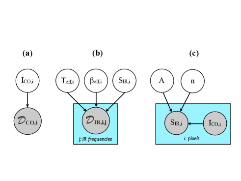
Figure 1: Example Directed Acyclic Graphs (DAG) showing conditional dependencies between parameters (white circles) and measured data (gray circles). (a) DAG indicating that the measured CO data $\mathcal{D_{\rm CO,i}}$ can be predicted given the true CO intensity $I_{{\rm CO},i}$. (b) DAG where $T_{\rm eff,i}$, $\beta_{\rm eff,i}$, and $S_{{\rm IR},i}$ determine the IR data $\mathcal{D_{\rm IR,i,j}}$ at each frequency $j$. (c) DAG where the data are simply the IR and CO intensities, which are conditionally dependent on the regression parameters $A$ and $n$. See Section 2.3.

Next, suppose we are solely interested in the dust spectrum parameters, $\Theta=(S_{{\rm IR},i},T_{{\rm eff},i},\beta_{{\rm eff},i})$, for a particular location $i$, given the IR data for all channels. The likelihood function for the spectral parameters is the product of IR likelihood factors given by equation (9), with the $S_{{\rm IR},ij}$ values computed using the spectrum parameters. For simplicity, we ignore the intensity calibration parameters for the moment. Then the likelihood function for the spectrum parameters is

$$p(\mathcal{D}|\Theta) =\prod_{j}k_{j}[S_{{\rm IR},ij}(\Theta)]$$

$$\propto\exp\left[-\frac{\chi_{{\rm IR},i}^{2}(\Theta)}{2}\right],$$ (11)

where $\chi_{{\rm IR},i}^{2}(\Theta)$ is the familiar goodness-of-fit measure,

$$\chi_{{\rm IR},i}^{2}(\Theta)=\sum_{j}\frac{[\log(\hat{S}_{{\rm IR},ij}/S_{\rm fid})-\log(S_{{\rm IR},ij}(\Theta)/S_{\rm fid})]^{2}}{\sigma_{j}^{2}}.$$ (12)

If a flat prior PDF is adopted for the spectrum parameters, the mode (the parameter vector that maximizes the posterior PDF) is the maximum likelihood estimate, which is the parameter vector that minimizes $\chi_{{\rm IR},i}^{2}(\Theta)$.

Figure 1(b) depicts the conditional structure of this use of Bayes’s theorem. The top nodes denote independent prior PDFs for the three parameters. The three arrows indicate that all three parameter values must be specified to predict the data. The five data nodes (for the five frequency channels) are depicted using a plate, a box with a label indicating repetition over a specified index (here the channel index, $j$). Crucially, a plate signifies that each case is conditionally independent of the others; that is, with $\Theta$ given, the probability for $\mathcal{D}_{2}$ (say) is independent of the values of the data in other channels.

Finally, suppose that the (true) CO intensity, $I_{{\rm CO},i}$, and total IR luminosity, $S_{{\rm IR},i}$, were measured precisely for $N$ pixels (i.e., the data are the precise values, rather than uncertain estimates from photometry). In this case, we could learn the dust-gas relationship parameters in equation (4), $\Theta=(A,n)$, via regression, i.e., using the $N$ pairs $(I_{{\rm CO},i},S_{{\rm IR},i})$, to infer the conditional expectation of $S_{{\rm IR},i}$ given $I_{{\rm CO},i}$ (and $\Theta$). The DAG in Figure 1(c) shows the conditional structure of this regression model.

Commonly, a regression analysis quantifies the scatter about the fit line. In the next section, we compare the results from the hierarchical modelling with a non-hierarchical approach which utilizes standard regression methods. If we suppose the scatter about the regression line is Gaussian with standard deviation $s$, the likelihood function for estimating $\Theta=(A,n)$ in this problem is a product of normal distributions for the residuals,

$$p(\mathcal{D}|\Theta) =\prod_{i=1}^{N}\frac{1}{s\sqrt{2\pi}}\exp\left\{-\frac{1}{2s^{2}}[\log(S_{{\rm IR},i}/S_{\rm fid})\right.$$ (13)

$$\qquad\left.\vphantom{\frac{1}{2s^{2}}}-A-n\log(I_{{\rm CO},i}/I_{\rm fid})]^{2}\right\}$$

$$\propto\frac{1}{s^{N}}\exp\left[-\frac{\chi_{{\rm LR}}^{2}(\Theta)}{2}\right],$$ (14)

where $\chi_{{\rm LR}}^{2}(\Theta)$ is the sum of squared residuals (normalized by $s^{2}$) that is minimized in least-squares linear regression (LR),

$$\chi_{{\rm LR}}^{2}(\Theta)=\sum_{i}\frac{[\log(S_{{\rm IR},i}/S_{\rm fid})-A-n\log(I_{{\rm CO},i}/I_{\rm fid})]^{2}}{s^{2}},$$ (15)

To analyze the CO-FIR data, we are ultimately interested in regression and estimation of $(A,n)$. However, we do not have precise $(I_{{\rm CO},i},S_{{\rm IR},i})$ pairs; we have CO and IR data, providing uncertain estimates of these quantities. Perhaps the simplest way forward is to ignore the $I_{{\rm CO},i}$ and $S_{{\rm IR},i}$ uncertainties (or hope they will “average out”), using the estimates as if they were precise values in a linear regression model like that depicted in Figure 1(c). But problems of this sort are well-studied in the statistics literature on measurement error and errors-in-variables problems, where it is known that, instead of averaging out, the uncertainties instead accumulate, producing inconsistent parameter estimates (i.e., estimates that converge to incorrect values as data accumulate). Multilevel or hierarchical models provide a flexible framework for full accounting of such uncertainties, avoiding these inconsistencies.

Here we build a hierarchical model by composing the three DAGs described above (but leaving the $I_{{\rm CO},i}$ and $S_{{\rm IR},i}$ nodes open in the regression DAG, since the true values of these quantities are uncertain). In our HB model for the CO and FIR data, the parameter space is large (and grows in size with the data); $\Theta$ includes the regression parameters, $(A,n)$, the uncertain CO and IR intensities, $(I_{{\rm CO},i},S_{{\rm IR},i})$, and spectral parameters for each pixel, $(T_{{\rm eff},i},\beta_{{\rm eff},i},S_{{\rm IR},i})$. Figure 2 shows the DAG connecting all of these quantities; the DAGs of Figure 1 appear as sub-structures within this HB model. Note that for the first two DAGs in Figure 1, we were focusing our attention on a single location (pixel); in the single-location analyses described above, we specified flat prior PDFs for $I_{{\rm CO},i}$ and the IR SED parameters (in the absence of better-motivated alternatives). In the HB model, we jointly analyze data from all locations. This enables us to learn about the population distributions for these parameters. We do so by parameterizing these distributions, e.g., adopting a log-normal distribution for $I_{{\rm CO},i}$ and a bivariate normal for $(T_{{\rm eff},i},\beta_{{\rm eff},i})$ (details are provided below). The uncertain parameters specifying these population distributions become additional nodes in the HB model, as shown in Figure 2; in HB terminology, these are hyperparameters. For more information on hierarchical Bayesian methods, we refer the reader to Gelman et al. (2004), Gelman & Hill (2007), and Kruschke (2011).

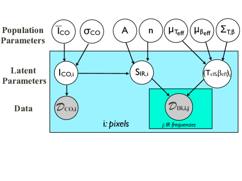
Figure 2: DAG showing the conditional dependencies between the estimated parameters and data of the hierarchical model described in Section 2. The highest level contains the global population, or hyper-, parameters such as the mean dust temperature ($\mu_{T}$), the $T_{\rm eff,i}$ and $\beta_{\rm eff,i}$ covariance matrix $\Sigma_{T,\beta}$, which includes their correlation ($\rho_{T,\beta}$), or the Kennicutt-Schmidt index ($n$). These parameters are required to estimate the other latent parameters occurring at the pixel level, denoted with a subscript $i$, and are located within the cyan box, or plate, in the DAG. The subscript $j$ refers to the frequency of the observed IR intensity, located within an additional plate. The dust surface density $\Sigma_{\rm d,i}$ can be evaluated given the other parameters (via eqn. 30), and is required to estimate the IR intensity $S_{i,j}$.

A DAG only specifies the qualitative structure of the HB model; to implement it, we must specify distributions (suitably conditioned) for every node. For instance, the DAG indicates that we need a distribution for the pair $(T_{{\rm eff},i},\beta_{{\rm eff},i})$ conditional on their mean values and the covariance matrix ($\mu_{T}$, $\mu_{\beta}$, $\Sigma_{T,\beta}$), independent of all other parameters. We model the dust $T_{\rm eff,i}$ and $\beta_{\rm eff,i}$ with a bivariate normal PDF. Therefore, that node of the DAG corresponds to a factor in the joint PDF:

$$\mathcal{P}(T_{\rm eff},\beta_{\rm eff}|\mu_{T},\mu_{\beta},\Sigma_{T,\beta})=\mathcal{N}(T_{\rm eff},\beta_{\rm eff}|\mu_{T},\mu_{\beta},\Sigma_{T,\beta}),$$ (16)

where $\mathcal{N}({\bf x}|{\bf S})$ is the bivariate normal PDF for ${\bf x}$ given means and covariance ${\bf S}$. We employ simpler, abbreviated standard statistical notation, so that equation (16) is written as

$$(T_{\rm eff},\beta_{\rm eff})^{T}|{\bf\mu_{T,\beta},\Sigma_{T,\beta}}\sim{\bf\mathcal{N}}({\bf\mu}_{T,\beta},{\bf\Sigma_{T,\beta}}),$$ (17)

where $({\bf x})^{T}$ is the transpose of the vector ${\bf x}$, and ${\bf\mu_{T,\beta}}=(\mu_{T},\mu_{\beta})^{T}$. Some parameters, such as the correlation between $T_{\rm eff,i}$ and $\beta_{\rm eff,i}$, $\rho_{T,\beta}$, are modeled with uniform distributions, denoted by $\mathcal{U}(min,max)$ spanning $min$ and $max$.

In order to evaluate the joint likelihood of all the parameters, we model the distributions of most parameters as normals. The quantities $A$, $n$, $\overline{I}_{\rm co}$ and ${\sigma}_{\rm co}$ are the population parameters describing the intercept and slope of the $S_{\rm IR}$$-$$I_{\rm CO}$ relationship (Eqn. 4), and the mean and standard deviation of the true CO intensity (in log space), respectively. Obtaining a reliable estimate for these quantities is one of the primary goals of the hierarchical fitting process. The distributions of the population parameters also require (hyper) priors. Again, we choose normal distributions with large variances. The choice of the mean values of these hyperpriors does not affect the posterior, again due to the large number of datapoints that constrain these parameters more than the priors. In our tests of the method described in the next section, we investigate the influence of the prior distributions when the underlying data are not normal.

For the CO and IR data nodes, we adopt log-normal likelihood functions as described above, in equations (8) and (9). We assign a population distribution to the CO intensities that is log-normal, specified by two hyperparameters (population distribution parameters): a mean, $\log\overline{I}_{\rm CO}$, and standard deviation, $\sigma_{\rm CO}$. We assign these parameters a normal and a uniform prior, respectively. Thus,

$$\log({I}_{\rm CO,i}/I_{\rm fid})|\log(\overline{I}_{\rm CO}/I_{\rm fid}),\sigma_{\rm CO} \sim\mathcal{N}(\log\overline{I}_{\rm CO}/I_{\rm fid},\sigma_{\rm CO}^{2}),$$ (18)

$$\log(\overline{I}_{\rm CO}/I_{\rm fid}) \sim\mathcal{N}(0,5),$$ (19)

$$\sigma_{\rm CO} \sim\mathcal{U}(0,2).$$ (20)

We treat each source’s temperature and power law index as drawn from a bivariate normal population distribution,

$$(T_{\rm eff},\beta_{\rm eff})_{i}^{T}|{\bf\mu_{T,\beta},\Sigma_{T,\beta}}\sim{\bf\mathcal{N}}({\bf\mu_{T,\beta}},{\bf\Sigma_{T,\beta}}).\\$$ (21)

The population mean temperature and index have normal hyperpriors;

$$\mu_{T} \sim\mathcal{N}(40,20),$$ (22)

$$\mu_{\beta} \sim\mathcal{N}(0,3).$$ (23)

We write the temperature-index covariance matrix in terms of the (marginal) standard deviations for temperature and index, and a correlation parameter, $\rho_{T,\beta}$:

$${\bf\Sigma_{T,\beta}}|\rho_{T,\beta},\sigma_{T},\sigma_{\beta}=\begin{bmatrix}\sigma_{T}^{2}&\rho_{T,\beta}\sigma_{T}\sigma_{\beta}\\ \rho_{T,\beta}\sigma_{T}\sigma_{\beta}&\sigma_{\beta}^{2}\end{bmatrix}.$$ (24)

We assign uniform priors to these three hyperparameters:

$$\rho_{T,\beta} \sim\mathcal{U}(-1,1),$$ (25)

$$\sigma_{T} \sim\mathcal{U}(0,50),$$ (26)

$$\sigma_{\beta} \sim\mathcal{U}(0,3).$$ (27)

Note that it is customary in non-hierarchical models to assign unknown standard deviations log-uniform priors (i.e., priors proportional to the inverse standard deviation). In a hierarchical setting, because of the weakened connection between hyperparameters and the data, such an assignment can unduly influence the posterior (even making it improper, i.e., unnormalizeable). Flat priors have better behavior while still remaining only weakly informative (Gelman et al., 2004).

Finally, we specify informative but broad priors on the offset ($A$) and slope ($n$) in the $\log(S)$–$\log(I)$ relationship,

$$A \sim\mathcal{N}(0,100),$$ (28)

$$n \sim\mathcal{TN}(0,4),$$ (29)

with $\mathcal{TN}(\cdot,\cdot)$ denoting a truncated normal, requiring the quantity to be greater than or equal to the specified mean (here requiring $n\geq 0$). These priors are motivated by previous observational studies, which always find and increasing $\Sigma_{\rm SFR}$ with $\Sigma_{\rm mol}$. We follow convention and assume constant conversions between FIR and $\Sigma_{\rm SFR}$, as well as CO and $\Sigma_{\rm mol}$. However, we do not favor any particular values for the conversion factors, hence employing a large range for the possible value of the offset ($A$) parameter.

The dust surface density can be computed from the modeled parameters described above:

$$\log\Sigma_{\rm d,i}|A,n,I_{\rm CO,i},T_{\rm eff,i},\beta_{\rm eff,i}=\\ A+n\log(I_{\rm CO,i}/I_{\rm fid})-\log\left(\int B_{\rm\nu}(T_{\rm eff,i})\kappa_{0}\left(\frac{\nu}{\nu_{0}}\right)^{\beta_{\rm eff,i}}d\nu\right)$$ (30)

With $\Sigma_{\rm d,i}$, $T_{\rm eff,i}$  and $\beta_{\rm eff,i}$, the true IR intensity at each pixel $i$ is given by Equation 1:

$${S}_{\rm i,j}|(T_{\rm eff},\beta_{\rm eff})_{i},\Sigma_{\rm d,i}=\\ \Sigma_{\rm d,i}\frac{2h\nu_{j}^{3}}{c^{2}}\kappa_{0}\left(\frac{\nu_{j}}{\nu_{0}}\right)^{\beta_{\rm eff,i}}\frac{1}{\exp(h\nu_{j}/k_{B}T_{\rm eff,i})-1}.$$ (31)

The reference opacity at $\nu_{0}$=230 GHz is assumed to be fixed at $\kappa_{0}=0.9$ cm² g^-1 (Ossenkopf & Henning, 1994).

We note that we do not favor any particular $\rho_{T,\beta}$  so it is modeled with a uniform distribution between $-$1 (fully anti-correlated) and 1 (exact correlation). We model the mean temperature and spectral index, $\mu_{T}$ and $\mu_{\beta}$, as normal distributions, with large variances for their priors, allowing the sampler to explore a wide range of possible values near typical ISM conditions. Given the large number of datapoints, the final estimates for $\mu_{T}$ and $\mu_{\beta}$ are not sensitive to these choices.

To carry out the hierarchical analysis, we use the Stan probabilistic programming language via its R language API (Stan Development Team, 2014).^, Stan performs efficient sampling of the parameters through a Hamiltonian Monte Carlo algorithm. We refer the reader to the manual and website for more information about the details of Stan.

3 Simulation Studies

To test the HB fitting method, we construct synthetic datasets and compare the posterior with the adopted underlying parameters. For some parameters, we also investigate the effect of choosing incorrect prior distributions, e.g. a truncated normal distribution for $I_{\rm CO}$ when the underlying distribution is in fact log-normal. In this section, we present and discuss the results from three such investigations, though we have performed the HB analysis on several realizations of the synthetic datasets. Here, we aim to demonstrate that the HB model described in Section 2 is properly implemented. We also illustrate that the HB analysis provides more accurate parameter estimates than a simple regression analysis. For the latter, we construct synthetic datasets for which the underlying parameters do not follow the distributions assumed in the HB model.

The synthetic datasets are characterized by five latent variables: $\log$ $\Sigma_{\rm d,i}$, $\log$ $S_{\rm IR}$, $\log$ $I_{\rm CO}$, $T_{\rm eff,i}$, and $\beta_{\rm eff,i}$. From these quantities and chosen observational uncertainties, we produce the observed CO and IR intensities, $\hat{I}_{\rm CO,i}$ and $\hat{S}_{\rm i,j}$. The first two columns of Tables 1 and 2 show the summary statistics of the most interesting hyperparameters of the synthetic datasets.

Figure 3 shows the distributions and bivariate relationships for the true values of the 5 individual pixel latent variables in synthetic dataset A. The panels on the diagonal display the histograms of each variable. The panels below the diagonal show the scatter-plots between the variables identified by its row and column position. Similarly, the correlation coefficient between the corresponding variables are shown in the panels above the diagonal. For synthetic dataset A, we choose distributions of the underlying parameters to match those in the HB modelling, as the aim of this initial test is verify that the HB model is implemented correctly. In Table 1, the second column lists the adopted values of the parameters in test dataset A. For each of the 75 replicates (or “pixels”) of this dataset, we include a 15% uncertainty to create the synthetic observed CO intensities, and a random 2% uncertainty on the IR intensity. For the calibrated errors, we employ 10% and 8% uncertainties for $\mathcal{C_{\rm PACS}}$, and $\mathcal{C_{\rm SPIRE}}$, respectively, corresponding to the estimated uncertainties from the PACS and SPIRE instruments (see Section 4.2).

Table 1: Adopted and HB Estimated Population Parameters for Synthetic Dataset A¹

Parameter	True Value	Posterior Mean	95% HPD
$\rho_{T,\beta}$	0.47	0.38	[0.18, 0.59]
$\mu_{T_{\rm eff}}$	25.0	25.1	[24.7, 25.6]
$\sigma_{T}$	2.1	2.2	[1.8, 2.6]
$\mu_{\beta_{\rm eff}}$	1.98	1.97	[1.91, 2.05]
$\sigma_{\beta}$	0.3	0.32	[0.26, 0.37]
$\log\overline{I}_{\rm CO}$	1.57	1.56	[1.52, 1.60]
$\sigma_{\rm CO}$	0.17	0.17	[0.14, 0.20]
$n$	1.5	1.49	[1.37, 1.63]
$A$	$-$2.00	$-$1.95	[$-$2.15, $-$1.75]

In sampling the posterior, we run three MCMC chains and ensure sufficient mixing and convergence by inspecting that the $\hat{R}$ values of all the population parameters are very close to one, and that the effective sample size is large (Gelman et al., 2004; Flegal et al., 2008). Since we are interested in 95% density intervals, we ensure that the effective sample sizes of the main population parameters of interest, $\rho_{T,\beta}$, $\mu_{\beta_{\rm T}}$, $\mu_{\beta_{\rm eff}}$, $n$, and $A$, are at least 3500, with corresponding $\hat{R}\approx 1$. We choose random initial values for the latent parameters, ensuring a wide range (e.g. $T_{\rm eff,i}$ between 10 and 50 K). For synthetic dataset A, we run the chains for 18,000 iterations, and the traceplots show that after $\sim$1000 draws the chains pass the $\hat{R}\approx 1$ convergence test.

The last two columns of Table 1 shows the posterior means and 95% highest posterior density (HPD) intervals. Clearly, the posterior means are very near the true underlying values, and the HPD bracket the adopted values. We have performed similar tests on additional synthetic datasets, each with slightly different underlying parameters. Since the HPD of the posterior brackets the true value, we can be confident of the HB model implementation in Stan.

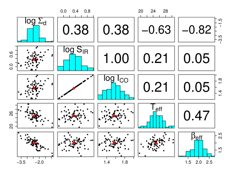
Figure 3: Distributions across pixel and bivariate relationships of quantities in synthetic dataset A. The diagonal panels label the variables associated with that row and column, and include their histograms. The upper triangle lists the correlation coefficient between the quantities in the same row and column. Panels in the lower triangle show the scatter plot of the corresponding data, with the red points indicating the mean values.

In order to explore the effect of the prior distributions, we consider datasets where the adopted distributions do not correspond to those assumed in the HB model. For this second test, we set $I_{\rm CO}$ to have a truncated normal distribution. As a result, $\log$$I_{\rm CO}$ is not normally distributed, and thereby differs from the model assumption. We choose a low value for $\overline{I}_{\rm CO}$ and a large variance. As we draw values for $I_{\rm CO,i}$, we discard any data with $I_{\rm CO,i}<0$. This truncation thereby directly affects the $S_{\rm IR}$ distribution. Eliminating replicates with $I_{\rm CO,i}<0$ also modifies the other latent variables. In addition, we draw $T_{\rm eff,i}$ from a uniform distribution, while keeping the normal distribution of $\beta_{\rm eff,i}$. With model misspecification, the distributions of the latent variables deviate from their chosen prior distributions in the HB model. Figure 4 shows the distributions and bivariate relationships of the underlying quantities in synthetic dataset B, which consists of 100 datapoints. We include correlated calibration and random uncertainties: 10% and 5% for the PACS bands, respectively, and 8% and 7% for the SPIRE bands. It is clear from Figure 4 that the synthetic quantities do not follow the distributions adopted in the priors of the HB model.

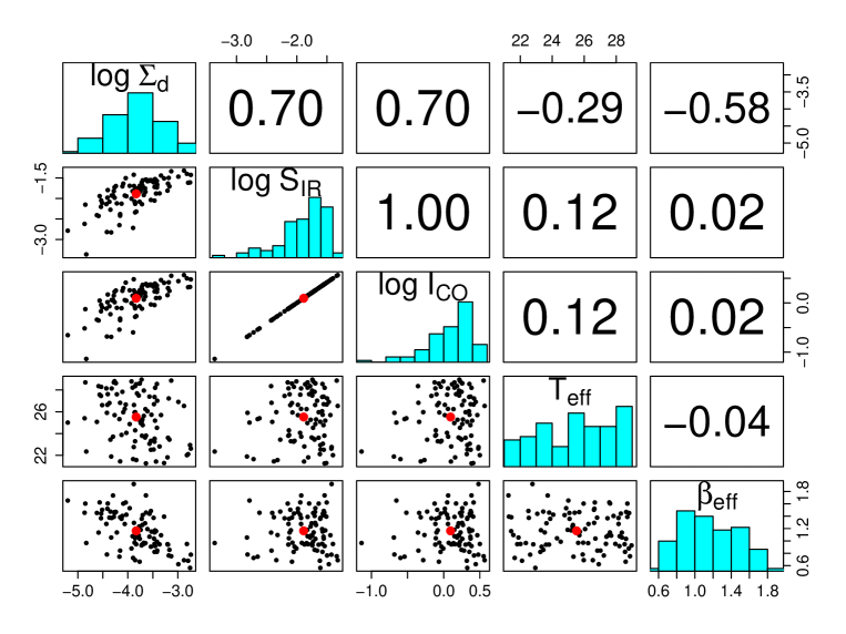
Figure 4: Relationships between quantities in synthetic dataset B. The panels are arranged in the same manner as Figure 3.

We choose initial parameter values and chain lengths similar to those employed for synthetic dataset A. We find that 18,000 iterations for each of the three chains display convergence for all parameters, including $\hat{R}\approx$1 and large effect sample sizes  $\buildrel>\over{\sim}$ 4000. Columns 1 - 4 of Table 2 lists the adopted values and the HB estimated values and their 95% HPDs of the key parameters in synthetic dataset B. As with test A, the 95% HPDs of each parameter includes the true values of dataset B, and the posterior means are similar to the true values.

Table 2: Intrinsic, HB, and RIME ($\chi^{2}$) Estimated Population Parameters for Synthetic Dataset B

Parameter	True Value	Posterior Mean	95% HPD	RIME Estimates
$\rho_{T,\beta}$	0.0	-0.03	[-0.32, 0.26]	$-0.22\pm 0.1$
$\mu_{T_{\rm eff}}$	25.3	25.5	[24.9, 26.1]	25.7$\pm 0.2$
$\sigma_{T}$	2.2	2.3	[1.8, 2.8]	2.2$\pm 0.3$
$\mu_{\beta_{\rm eff}}$	1.24	1.18	[1.10, 1.25]	1.21$\pm 0.03$
$\sigma_{\beta}$	0.33	0.31	[0.25, 0.37]	0.32$\pm 0.03$
$\log\overline{I}_{\rm CO}$	0.15	0.09	[0.02, 0.16]	-
$\sigma_{\rm CO}$	0.28	0.32	[0.28, 0.37]	-
$n$	1.20	1.20	[1.16, 1.25]	1.14$\pm 0.05$
$A$	$-$2.00	-1.99	[-2.04, -1.94]	-1.99$\pm 0.07$

We compare the HB results with parameters estimated via commonly employed methods. For the latter, we perform a simple regression ignoring measurement error, or RIME, analysis of synthetic dataset B. For each pixel, we fit the modified blackbody to the five intensities by minimizing equation (12) and then perform linear regression between the estimated $\log$$S_{\rm IR}$ and $\log\hat{I}_{\rm CO}$, described by equation (15). We simulate a large number of datasets with the same properties as synthetic dataset B, including a correlated term for the calibration uncertainty and a random noise term. We then perform a RIME analysis of each realization. We compare the resulting sampling distributions of the fit parameters to the estimates from the HB model.

Figure 5 shows the RIME estimates, HB posterior mean, and the true values of $T_{\rm eff,i}$ and $\beta_{\rm eff,i}$. The last column of Table 2 shows the best RIME parameter estimates and the $2\sigma$ uncertainty of the underlying parameters from the sampling distribution. The RIME results indicate an anti-correlation between $T_{\rm eff,i}$ and $\beta_{\rm eff,i}$, with $\rho_{T,\beta}$=$-$0.23. Since the degeneracy between $T_{\rm eff,i}$ and $\beta_{\rm eff,i}$ is explicitly treated in the HB method via the modeling of $T_{\rm eff,i}$ and $\beta_{\rm eff,i}$ with a bivariate normal distribution, the HB method is more reliable in estimating their correlation (Kelly et al., 2012).

We can quantify the fits by computing the mean squared error (MSE) of the RIME estimates and HB samples. The MSE of $\beta_{\rm eff,i}$ of both methods are similar, 0.03. However, the MSE of $T_{\rm eff,i}$ from the RIME method is 2.86, which is about 6% higher than the mean MSE of 2.69 provided by the HB analysis. Even though the HB estimate misspecifies the population parameters, it is able to provide more accurate estimates of $T_{\rm eff,i}$ than the RIME point estimates.

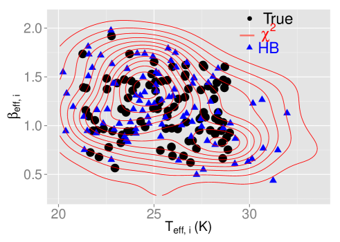
Figure 5: Comparison of estimated $T_{\rm eff,i}$ and $\beta_{\rm eff,i}$ from the HB (blue) and $\chi^{2}$ point estimate methods (red contours, computed via kernel density estimation). The black points show the true values in synthetic dataset B.

From the RIME estimates of $T_{\rm eff,i}$, $\beta_{\rm eff,i}$  and $\Sigma_{\rm d,i}$, we can integrate the SED defined by these quantities to obtain estimates of $S_{\rm IR}$. Figure 6 shows the comparison of the true and fit $I_{\rm CO}$ $-$ $S_{\rm IR}$ relationships. The blue lines show 20 random draws from the HB posterior. The red points show the RIME estimated $S_{\rm IR}$ plotted along with the observed (i.e. noisy) $\hat{I}_{\rm CO}$ values. This differs from the HB model, which explicitly estimates the true values of $I_{\rm CO}$; these values are used in the evaluation of the $I_{\rm CO}$ $-$ $S_{\rm IR}$ relationship. The RIME estimate of the slope of $I_{\rm CO}$ - $S_{\rm IR}$ is 1.13, with $2\sigma$ uncertainty 0.05, as indicated in Table 2. This value is flatter than the underlying value $n$=1.2, even at the $2\sigma$ level. As shown by numerous previous works, when measurement uncertainties in the predictor are not treated in the linear regression, the fit slope will be biased towards 0 (see e.g. Akritas & Bershady, 1996; Carroll et al., 2006; Kelly, 2007). Note also that a linear regression on observations with relative IR noise levels  $\buildrel>\over{\sim}$ 10% will estimate a slope with more bias than the results from synthetic dataset 2. The HB estimate of $n$, on the other hand, explicitly treats measurement uncertainties in all observables, thereby leading to significantly more accurate parameter estimate than the $\chi^{2}$ value.

We have also checked the relationship between each IR band and $\hat{I}_{\rm CO}$. Fits involving any individual IR intensities usually underestimates the underlying slope, with the magnitude of the bias depending on the noise characteristics, as well as the true values of the parameters. In general for higher noise levels, we have found that the estimated slopes using solely the longer wavelength intensities perform worse than those at shorter wavelengths. Such tests suggest that, similar to the RIME SED fits, employing any individual intensity will likely lead to an underestimate of the slope of the FIR $-$ CO relationship.

We have also performed a test on a synthetic dataset where the $T_{\rm eff,i}$ $-$ $\beta_{\rm eff,i}$ distribution is not bivariate normal. As we show in the next Section, for the LMC the $T_{\rm eff,i}$ $-$ $\beta_{\rm eff,i}$ distribution has curvature, indicating that the model is mis-specified. To assess whether such mis-specification unduly influences the estimates of the main parameters of interest, such as $n$, we construct a sythetic dataset using the posterior mean of $T_{\rm eff,i}$ and $\beta_{\rm eff,i}$ from the LMC. We create all the other latent parameters as in Synthetic Dataset B, and perform the HB model of this synthetic dataset. We find that the 95% HPD brackets the true value of the underlying latent parameters. A rigorous test of such mis-specification (e.g., verifying approximate coverage of 95% regions) would require the execution of the HB model on thousands of such sythetic datasets. Since this is unfeasible, our limited tests considering only 5 synthetic datasets suggests that, broadly speaking, the results are robust to mis-specifying the $T_{\rm eff,i}$ and $\beta_{\rm eff,i}$ distribution.

Before concluding this section, we stress that though the HB model employs the simple assumption of a single (effective) temperature and spectral index, the total FIR luminosity estimate is not significantly affected by this constraint. To verify this, we have constructed simple models with an additional colder dust component, with temperatures in the range 5 $-$ 15 K, and with surface densities that are 5 $-$ 20 larger than the warm component, and fit the single-component SED to the emergent IR intensities at the Herschel wavelengths. Though the fit parameters can be discrepant from true temperatures and spectral indices regardless of which component dominates the emergent SED, the estimated integrated SED recovers $S_{\rm IR}$ to a very high degree of accuracy, often within 0.5%. This demonstrates the robustness of $S_{\rm IR}$, and that the fit temperature and spectral index should only be interpreted as “effective” parameters. Therefore, $\beta_{\rm eff,i}$, which determines the Rayleigh-Jeans tail of the fit SED, must be understood only as the appropriate numerical parameter required to reproduce the observed intensities within the single-component SED model. For an investigation focusing on the properties of dust along each LoS, additional IR fluxes in the Rayleigh-Jeans tail of the SED would be necessary to constrain the $\beta_{\rm eff,i}$, and a multi-component fit may better recover the observed trends. In this study, we are primarily interested in the total IR luminosity that is not strongly affected by the precise parameter estimates of $\beta_{\rm eff,i}$, so we can be confident that the information provided by the Herschel images is sufficient for estimating $S_{\rm IR}$.

In summary, the tests on synthetic data demonstrate that the HB model performs well under certain conditions. For synthetic dataset A the underlying distributions matched those assumed in the HB model, resulting in a highly accurate and precise posterior. Synthetic dataset B includes variables with distributions which are discrepant from those assumed in the HB model. Nevertheless, the HB method is able to recover the underlying latent parameters within the 95% HPD. We note that a RIME fit to the intensities of synthetic dataset B recovers the mean values and marginal distributions of $T_{\rm eff,i}$, $\beta_{\rm eff,i}$  and $S_{\rm IR}$. However, both $\rho_{T,\beta}$ and $n$ are significantly underestimated. Such discrepancies advocate for employing a hierarchical modelling technique, which relaxes the strong assumption of independence between $T_{\rm eff,i}$ and $\beta_{\rm eff,i}$ adopted in the RIME fit.

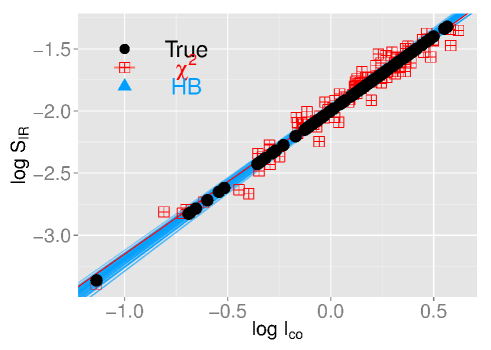
Figure 6: Comparison of estimated and true $I_{\rm CO}$ $-$ $S_{\rm IR}$ relationships for test dataset B. The blue lines are 20 random draws from the HB posterior, and the red points show the $\chi^{2}$ estimates of $S_{\rm IR}$ at the observed values of $\hat{I}_{\rm co}$, with the red line depicting the best fit. The black points show the true values in synthetic dataset B.

4 Application: The Large and Small Magellanic Clouds

4.1 Observations

As an initial application of the HB method on real data, we analyze the dust and gas properties of the Magellanic Clouds using the Herschel HERITAGE key project FIR data (Meixner et al., 2013), in conjunction with CO $J=1-0$ NANTEN observations (Mizuno et al., 2001a, b). We convolve all maps to a common resolution of 100 pc, since we are interested in the large scale properties of the ISM. We consider those pixels with $I_{\rm CO}$ $>0$ K km s^-1. Given these constraints, the number of independent pixels we analyze in the SMC and LMC is 132 and 1584, respectively. To illustrate the maps we employ for this work, Figure 7 shows the LMC and SMC map at 100 pc scales from the 100, 160, and 250 µm observations, with the contours displaying the CO peaks.

We have quantified the spatial correlation of residuals between neighbouring pixels as a result of the beam convolution at the 100 pc resolution we employ. We have measured the correlation coefficient of the residual values of neighbouring 100$\times$100 pc² pixels in synthetic data with similar resolution and gridding to Herschel images. We find that the residuals can be correlated by upto $\sim$20 per cent between adjacent pixels. We have checked that this correlation likely does not influence our results as we have run the HB model on every other pixel of the LMC maps, in which case the employed pixels are uncorrelated, and have recovered similar results to that from the full maps. Therefore, the $\sim$20 per cent introduced correlation between adajacent pixels is sufficiently small such that we can confidently apply the HB model, assuming conditional independence between pixels.

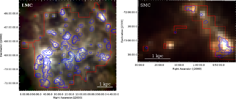
Figure 7: Three-color image of the LMC and SMC at 100 pc scale from the 100, 160, and 250 µm Herschel observations. The blue contours show the CO intensities at by 0.2, 0.3, 0.5, 1 and 2 K km s^-1 for the LMC, and 0.1, 0.2, 0.3, 0.5 and 1 K km s^-1 for the SMC. The red box demarcates the observed region of the CO maps

4.2 Uncertainties and Photometric colour corrections

The HB model requires (fixed) values for the standard deviations of the correlated and uncorrelated uncertainties discussed in Section 2.2 . Following Müller et al. (2011), we set the following for the PACS (j=1 or 2, corresponding to 100 and 160 µm) uncertainties:

$$\mathcal{C_{\rm PACS}}\sim\mathcal{N}(0,\log(1.1))$$ (32)

$$\sigma_{\rm j={1\,or\,2}}=\log(1.02).$$ (33)

As reported in Griffin et al. (2013) and Bendo et al. (2013), for SPIRE (j=3, 4, or 5, corresponding to 250, 350, and 500 µm) we set

$$\mathcal{C_{\rm SPIRE}}\sim\mathcal{N}(0,\log(1.08))$$ (34)

$$\sigma_{\rm j={3,\,4\,or5}}=\log(1.015).$$ (35)

To compare the model SEDs with the observations, the analytic modified blackbody (MBB) curves should be convolved with the PACS and SPIRE filter response functions to produce synthetic Herschel photometry. In order to speed up the calculations and because the corrections only depend on the shape of the SED, we pre-calculate colour corrections ($CC$) factors for MBBs with a range of $T$ and $\beta_{\rm eff}$ values. The correction factors are defined as F_ν,Herschel = $CC_{\nu}\cdot$F_ν,mono, where F_ν,Herschel is the flux-density value as measured by the Herschel bolometers and F_ν,mono is the monochromatic flux-density, i.e. the value in the perfectly sampled model SED, at the reference wavelength. We calculate $CC$ values for 15 K$\leq T\leq$40 K and 0$\leq\beta_{\rm eff}\leq$3. In general the correction factors are relatively small but significant. Over the immediate range of interest (20 K$<$T$<$30 K and 0.5$<\beta_{\rm eff}<$2) the maximum amplitude ($\|CC-1\|$) of the correction is 0.02, 0.05, 0.05, 0.07 and 0.11 for the 100, 160, 250, 350 and 500 $\mu$m filters, respectively.

Inside stan, the colour correction factors are specified as a second order polynomial in $T$ and $\beta_{\rm eff,i}$ whose parameters have been determined by fitting a 2D plane to the $CC$ values using the IDL routine SFIT.

4.3 Results

Figure 8 shows the marginal means of the estimated $T_{\rm eff,i}$ and $\beta_{\rm eff,i}$ in each pixel of the SMC and LMC. Tables 3 and 4 display the posterior mean and 95% HPDs of the location and scale parameters of the $T_{\rm eff,i}$ $-$ $\beta_{\rm eff,i}$ distributions. We find that the distributions of $T_{\rm eff,i}$ and $\beta_{\rm eff,i}$ are rather different between the two galaxies, with the LMC showing a larger anti-correlation (mean value $\overline{\rho}_{T,\beta}=-0.74$) than the SMC ($\overline{\rho}_{T,\beta}=-0.15$). In general, the galaxies also have different mean temperatures and spectral indices location parameters, with $\mu_{T_{\rm eff}}\approx$ 24.3 in the LMC and $\approx$ 25.7 K in the SMC. The $\mu_{\beta_{\rm eff}}\approx$1.32 for the LMC, and $\approx$0.99 for the SMC.

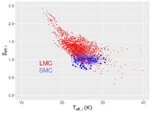
Figure 8: The $T_{\rm eff,i}$$-$ $\beta_{\rm eff,i}$ relationships for the LMC (red) and SMC (blue).

Table 3: HB Estimated $T_{\rm eff,i}$ - $\beta_{\rm eff,i}$ parameters for the LMC

Parameter	Posterior Mean	95% HPD
$\rho_{T,\beta}$	-0.74	[-0.76, -0.7]
$\mu_{T_{\rm eff}}$	24.3	[24.1, 24.5]
$\sigma_{T}$	4.3	[4.1, 4.4]
$\mu_{\beta_{\rm eff}}$	1.32	[1.31, 1.33]
$\sigma_{\beta}$	0.28	[0.27, 0.29]

Table 4: HB Estimated $T_{\rm eff,i}$ - $\beta_{\rm eff,i}$ parameters for the SMC

Parameter	Posterior Mean	95% HPD
$\rho_{T,\beta}$	-0.15	[-0.34, 0.03]
$\mu_{T_{\rm eff}}$	25.7	[25.4, 26.0]
$\sigma_{T}$	1.8	[1.6, 2.0]
$\mu_{\beta_{\rm eff}}$	0.99	[0.97, 1.00]
$\sigma_{\beta}$	0.1	[0.09, 0.12]

As is evident from Figure 8, the $T_{\rm eff,i}$ $-$ $\beta_{\rm eff,i}$ distribution is not bivariate normal, especially for the LMC. This indicates that this aspect of the HB model is mis-specified, and the HB parameter $T_{\rm eff,i}$ $-$ $\beta_{\rm eff,i}$ estimates do not have a straightforward interpretation as moments of the population distribution; rather, they are moments of a bivariate normal approximation to that distribution. Nevertheless, from the simulation studies described in Section 3, we can be confident that the other estimated parameters are not strongly affected by this specification. One possible reason for the curved $T_{\rm eff,i}$ $-$ $\beta_{\rm eff,i}$ relationship is that the single-temperature SED does not accurately reproduce the shape of the observed spectrum, as we further discuss below.

Table 5: HB Estimated Parameters for the LMC

Parameter	Posterior Mean	95% HPD
$\log\overline{I}_{\rm CO}$	-0.59	[-0.61, -0.57]
$\sigma_{\rm CO}$	0.32	[0.28, 0.36]
$n$	1.25	[1.11, 1.38]
$A$	$-$2.5	[$-$2.6, $-$2.4]

Table 6: HB Estimated Parameters for the SMC

Parameter	Posterior Mean	95% HPD
$\log\overline{I}_{\rm CO}$	-0.76	[-0.82, -0.69]
$\sigma_{\rm CO}$	0.21	[0.17, 0.26]
$n$	1.47	[1.21, 1.72]
$A$	$-$2.1	[$-$2.3, $-$2.0]

The HB estimates of $T_{\rm eff,i}$ and $\beta_{\rm eff,i}$ in the Magellanic Clouds are comparable to previous estimates. Aguirre et al. (2003) also found that the mean spectral index in the SMC is lower than in the LMC. The absolute values of their estimates differ from those we estimate here, in part because they analyze all emission from the galaxies, whereas we only consider dense regions where CO is detected.

To illustrate that the HB modelling has accurately reproduced the observed data, we show two sample SEDs from each galaxy in Figures 9 and 10. The models and data correspond to the regions with some of the highest and lowest $S_{\rm IR}$ from each galaxy. The figures show the observed IR intensities, as well as the predicted intensities at the corresponding wavelengths. Note that the offset between the prediction and data from the model SEDs, especially at the highest frequencies, is expected, primarily due to the color corrections described in Section 4.2, and to a lesser extent the correlated uncertainties. The observations fall within the expected range of the predicted intensities, indicating that the HB method accurately recovers the observed data.

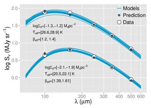
Figure 9: Example SED fits of two pixels in the LMC. These pixels correspond to regions that have the largest and smallest $S_{\rm IR}$. The lines are random draws from the posterior, and the blue points with errorbars show the mean Herschel predicted intensities with $2\sigma$ uncertainties. The slight offsets between the predictions and the model SEDs are due to the calibration uncertainties and color corrections. The white circles show the observed intensities ($\hat{S}_{\rm i,j}$). The legend below each set of SEDs shows the 95% HPDs of the fit parameters.

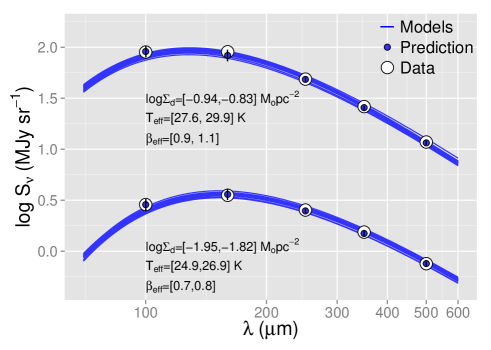
Figure 10: SED fits in pixels among the highest and lowest $L_{\rm IR}$ in the SMC. The model, predictions, and observed data are marked in the same fashion as Figure 9.

The differences in $\rho_{T,\beta}$ may be due to a number of possible variations in the structure of the ISM between the SMC and LMC . For instance, temperature gradients along the LoS may induce spurious correlations (e.g. Shetty et al., 2009b; Malinen et al., 2011; Juvela & Ysard, 2012; Veneziani et al., 2013; Gordon et al., 2014). There may be contrasting $T_{\rm eff,i}$ gradients, either in extent or magnitude, in the Magellanic Clouds leading to the difference in $\rho_{T,\beta}$. Other possibilities are that the dust-to-gas ratio and 500 µm excess may vary(e.g. Bernard et al., 2008; Roman-Duval et al., 2010; Gordon et al., 2014). Though measurement uncertainties can produce an artificial anti-correlation due to the degeneracy between $T_{\rm eff,i}$ and $\beta_{\rm eff,i}$, (e.g. Blain et al., 2003; Dupac et al., 2003; Shetty et al., 2009a), the HB method explicitly models the $T_{\rm eff,i}$$-$$\beta_{\rm eff,i}$ correlation and accurately accounts for noise, thereby reducing this effect (see Kelly et al., 2012). Other violations of model assumptions may also produce an artificial anti-correlation, such as a multiple dust components along the LoS leading to SEDs with a broken power-law Rayleigh-Jeans tail, and may be responsible for the apparent deviation of the LMC points from a bivariate normal distribution in Figure 8. As we have employed the same assumptions in modelling both Magellanic Clouds, the estimated differences in the $T_{\rm eff,i}$$-$ $\beta_{\rm eff,i}$ indicates the presence of fundamental differences in the dust characteristics of the LMC and SMC.

Tables 5 and 6 display the HB estimated parameters related to the $S_{\rm IR}$ $-$ $I_{\rm CO}$ of the LMC and SMC. Figure 11 shows 50 random draws of the $I_{\rm CO}$$-$$S_{\rm IR}$ relationship for both galaxies. The slopes of the two galaxies are similar; the posterior mean value of $n$ is 1.3 and 1.5 for the LMC and SMC, respectively, with overlap in the 95% HPDs. On the other hand, the intercepts are clearly different. Per unit $I_{\rm CO}$, the SMC has a $\sim$0.4 dex higher $S_{\rm IR}$ than the LMC. This difference is likely associated with the lower metallicity of the SMC, 0.2 Z_⊙, compared to 0.5 Z_⊙ of the LMC. If $S_{\rm IR}$ is a faithful tracer of the star formation rate, these results suggest that the star formation rate per unit $I_{\rm CO}$ is higher in the SMC by the same $\sim$0.4 dex factor. Numerous previous observations have shown such trends for lower metallicity systems (e.g. Taylor et al., 1998; Bolatto et al., 2011; Leroy et al., 2007; Cormier et al., 2014). The salient difference is in the ability to trace the star forming ISM with CO. In lower metallicity environments, there is a dearth of CO, so a given $I_{\rm CO}$ would be associated with a higher SFR compared to the higher metallicity case (Maloney & Black, 1988; Wolfire et al., 2010; Glover & Mac Low, 2011; Shetty et al., 2011a, b; Glover & Clark, 2012; Clark & Glover, 2015). Additionally, regions with higher atomic densities, will contain more dust. Therefore, dust emission should be correlated with total (atomic + molecular) gas density, and the offsets between the galaxies in Figure 11 may be partially due to the variations in total gas density, in addition to the metallicity differences.

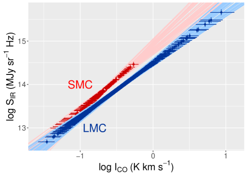
Figure 11: $I_{\rm CO}$$-$ $S_{\rm IR}$ relationship in the LMC and SMC (50 random draws from the posterior). Colored lines depict draws of regression lines from the marginal posterior distribution for $(A,n)$ for the SMC (red) and LMC (blue). Points with error bars show the marginal posterior means and marginal (1-D) 95% HPD regions for $(\log I_{\rm CO},\log S_{\rm IR})$ for each pixel in the two images.

The mean dust temperature is clearly larger in the SMC than the LMC, contributing to the overall increase in $S_{\rm IR}$ (at a given $I_{\rm CO}$). Such higher temperatures are observed in other lower metallicity systems (e.g. Rémy-Ruyer et al., 2013). Figure 12 shows the posterior mean relationship between $T_{\rm eff,i}$ and $I_{\rm CO}$. In the LMC, at large $I_{\rm CO}$ $\buildrel>\over{\sim}$ 0.5 K km s^-1, there is strong evidence that $T_{\rm eff,i}$ increases from $\approx$ 20 K to $>$30 K where $I_{\rm CO}$ $\approx$ 3 K km s^-1. This increase in dust temperature is likely due to radiation from young stars embedded in the dense molecular medium. At lower densities, we also find high $T_{\rm eff,i}$ values. Although this may be due to a decline in self-shielding, in the regions with the lowest $I_{\rm CO}$ the signal is close to the noise levels, so we should be careful not to over-interpret these data. At intermediate $I_{\rm CO}$, there is a large range in $T_{\rm eff,i}$, which is indicative of a mix of dense star forming regions, diffuse gas, and all material at intermediate densities. The SMC does not portray any strong trends as the $T_{\rm eff,i}$ estimates span a smaller range, though there is some hint of an increase in $T_{\rm eff,i}$ at the highest $I_{\rm CO}$.

One question is to what extent the dust surface density estimates affect $S_{\rm IR}$. Figure 13 shows the posterior mean of the $\Sigma_{\rm d,i}$ $-$ $I_{\rm CO}$ trends in the SMC and LMC. Again, there is an unambiguous offset, with the SMC showing larger $\Sigma_{\rm d,i}$ per unit $I_{\rm CO}$. As discussed, the lower metallicity in the SMC results in fewer CO molecules for a given dust surface density. Therefore, it is the combination of both higher temperatures and higher surface densities per unit CO intensity, both due to the lower metallicity in the SMC, which leads to the higher normalisation in the $S_{\rm IR}$$-$ $I_{\rm CO}$ trend shown in Figure 11.

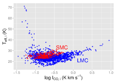
Figure 12: $I_{\rm CO}$$-$ $T_{\rm eff,i}$ relationship in the LMC (blue) and SMC (red). In order to better reveal the contrast between the Magellanic Clouds, we do not show contours for the LMC data. The points show $I_{\rm CO}$ and $S_{\rm IR}$ at each pixel from the mean of the posterior.

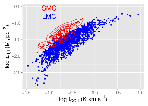
Figure 13: Example $I_{\rm CO}$$-$ $\Sigma_{\rm d,i}$ relationship in the LMC and SMC.

The HB model provides estimates of all the latent variables that determine the observed CO and IR intensities. Figure 14 shows the modeled distributions and bivariate correlations of these variables from the LMC. The displayed model corresponds to the posterior mean. Though there are clearly strong trends between many of the variables besides the bivariate relationships discussed above, as we discuss in the next section, interpreting such correlations requires a complete consideration of the key assumptions that enter the model.

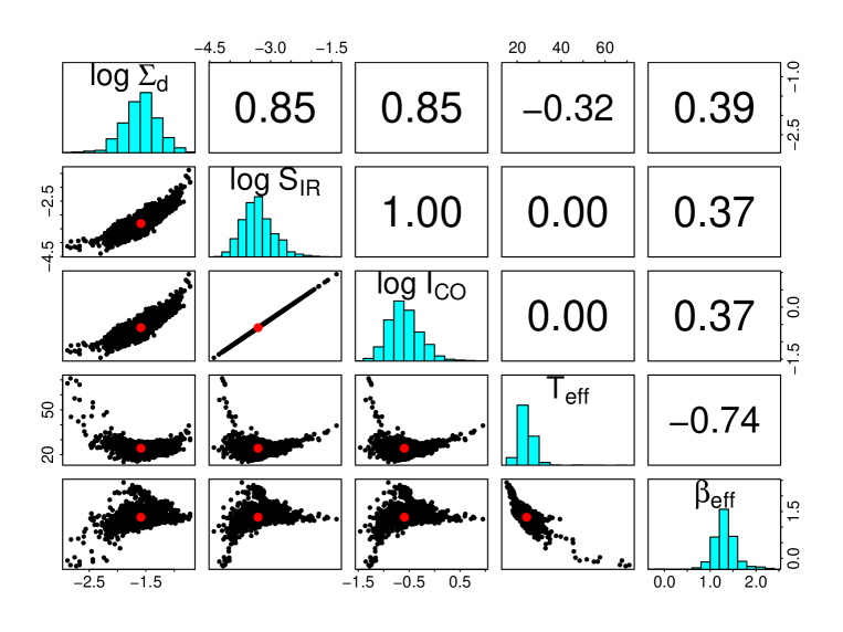
Figure 14: Modelled relationships and distributions between the latent variables in the LMC. The panels are arranged in the same manner as Figure 3.

5 Discussion

The HB modeling of dust SEDs and the dust - molecular gas relationship on 100 pc scales has revealed some interesting comparative features of the LMC and SMC. There is a strong anti-correlation between $T_{\rm eff,i}$ and $\beta_{\rm eff,i}$ in the LMC, with the SMC portraying a weaker anti-correlation, which may even be uncorrelated. Further, the slopes of $I_{\rm CO}$$-$ $S_{\rm IR}$ relationship are nearly identical, while $S_{\rm IR}$ in the SMC is larger by a factor of $\sim$3 at any given $I_{\rm CO}$. These results suggest that there are some fundamental differences in the properties of the dust and gas between the galaxies.

Though the estimated $\rho_{T,\beta}$ is significantly different between the LMC and SMC, we should be careful to draw too strong a conclusion from this result. Since the SED model does not account for multiple components, the estimated $\beta_{\rm eff,i}$ does not necessarily correspond to the underlying spectral indices of any of the components along the LoS. Rather, it should be considered a convenient numerical parameter necessary for fitting the SED model to the observations. As $S_{\rm IR}$ is not sensitive to the estimate of $\beta_{\rm eff,i}$, the modelled $I_{\rm CO}$$-$ $S_{\rm IR}$ also does not strongly depend on $\beta_{\rm eff,i}$. The SED modelling results indicate that there is some fundamental difference in the properties of dust, but further analysis is necessary to identify the cause of these differences. Possible causes may be associated with differences in the magnitude of the 500 µm excess, which is not modelled here, the dust-to-gas ratio (e.g. Gordon et al., 2014; Roman-Duval et al., 2014), and/or the dominance of the trend of some subset of the data (e.g. at low or high $T_{\rm eff,i}$). We have performed the HB fit to the SMC data excluding the 500 µm observation, but the resulting correlation and distributions are similar, suggesting that any 500 µm excess is not unduly affecting the estimated correlations in the high density regions traced by CO. More in-depth analysis of the observed IR maps may favor one of these or perhaps even other causes for the contrast in $\rho_{T,\beta}$, and whether the metallicity difference between the LMC and SMC is a significant contributing factor.

That the estimated value of $n$ in both galaxies are (approximately) equivalent may be indicative of a key similarity in the LMC and SMC. If $S_{\rm IR}$ is considered to be a linear tracer of $\Sigma_{\rm SFR}$  and $I_{\rm CO}$ is a faithful tracer of $\Sigma_{\rm mol}$, then the HB results suggests that the increase in the rate of star formation towards denser regions is similar in the LMC and SMC despite their difference in metallicity.

Analyses of the KS relationship on large scales in normal disk galaxies have revealed a range in $n$, with many galaxies portraying a sub-linear $\Sigma_{\rm SFR}$$-$$\Sigma_{\rm mol}$ relationship (e.g. Blanc et al., 2009; Ford et al., 2013). In fact, when using the single 24 µm intensity or its combination with UV observations, many galaxies in the HERACLES and STING surveys favor a sub-linear KS relationship, with significant galaxy-to-galaxy variations (Shetty et al., 2013, 2014b). Shetty et al. (2014a) interpret these and other observational results as evidence for a substantial amount of non star-forming molecular gas traced by CO, with this diffuse gas fraction consisting of at least 30% of the total molecular content (see also Wilson et al., 2012; Caldú-Primo et al., 2013; Pety et al., 2013). Recent analyses of the Milky Way further supports the presence of a significant diffuse molecular component (Roman-Duval et al., 2016; Liszt et al., 2010). Most of the extra-galactic results utilized monochromatic SFR tracers, which could contribute to the differences between the estimated indices from those investigations and those presented here.

Another explicit difference is that the metallicities of the Magellanic Clouds are significantly lower than those of the normal spiral galaxies. That the Magellanic Clouds have a super-linear KS relationship may be due to their lower metallicity. In low metallicity systems, higher levels of photodissociation results in a dearth of CO traced diffuse molecular gas compared to the normal spirals (e.g. Cormier et al., 2010; Schruba et al., 2012; Glover & Clark, 2012). Most regions with sufficient amounts of CO coincide with the locations of star formation. Applying the HB model to extra-galactic surveys will further reveal any trends between the KS index and other galaxy properties, and will allow for a more direct comparison with the results presented here. Worthwhile comparisons of systems with diverse metallicities involving dust SEDs would also require consideration of the fraction of young stellar radiation that does not heat the dust, which is estimated to be higher in the Magellanic Clouds (see Lawton et al., 2010).

Such investigations on a larger sample of galaxies should further reveal how well the dust properties may be associated with other characteristics of the ISM, such as the gas density, metallicity, and/or galaxy type. In these forthcoming analyses, however, we need to ensure that the model assumptions are fully considered in the interpretations. For instance, in this work we model the dust emission with single-component SEDs. As we are focusing on the dust and gas properties on large scales (100 pc), there is most certainly temperature variations along the LoS. Indeed, recent investigations on SED modelling on smaller scales have suggested that models with multiple dust components can better reproduce the observed IR emission (either with varying $T_{\rm eff,i}$, $\beta_{\rm eff,i}$, or both, see e.g. Galliano et al., 2011; Gordon et al., 2014). Future efforts including a consideration of temperature variations may provide additional insights into the large scale ISM.

6 Summary

We have introduced a hierarchical Bayesian (HB) method to analyze FIR and CO observations. The HB method estimates parameters of the dust SED; using estimates of the dust surface density $\Sigma_{\rm d,i}$, a single temperature $T_{\rm eff,i}$ and spectral index $\beta_{\rm eff,i}$, the method calculates the integrated FIR intensity $S_{\rm IR}$ at each pixel. Furthermore, the method simultaneously estimates the linear regression parameters of the $\log$ $S_{\rm IR}$ $-$ $\log$ $I_{\rm CO}$ relationship. When assuming that $S_{\rm IR}$ and $I_{\rm CO}$ faithfully trace the star formation rate $\Sigma_{\rm SFR}$ and molecular gas surface density $\Sigma_{\rm mol}$, respectively, the slope of this relationship is the Kennicutt-Schmidt index.

We test the HB method on synthetic datasets (Section 3). Even when the distributions of some key latent parameters are not normal, which is assumed in the HB model, the range in estimated parameters include the true underlying values. We also compare the HB results with common non-hierarchical techniques. Due to the degeneracy between $T_{\rm eff,i}$ and $\beta_{\rm eff,i}$ in the SED, the $\chi^{2}$ fit produces a $T_{\rm eff,i}$$-$ $\beta_{\rm eff,i}$ distribution that is biased towards an anti-correlation. The HB method explicitly treats the correlation between $T_{\rm eff,i}$ and $\beta_{\rm eff,i}$ among all pixels, and we demonstrate the posterior accurately recovers $\rho_{T,\beta}$. Moreover, a $\chi^{2}$ fit to the relationship between $I_{\rm CO}$ and $S_{\rm IR}$, or any individual IR intensity, is biased towards smaller slopes. This occurs in part because the $\chi^{2}$ analysis overestimates $S_{\rm IR}$ at low densities.

We apply the HB fit to Herschel IR and NANTEN CO maps of the LMC and SMC at 100 pc scales. The main results of this first application of the HB methods are as follows:

1) We find a stronger negative correlation between $T_{\rm eff,i}$ and $\beta_{\rm eff,i}$ in the LMC, with $\rho_{T,\beta}$$\approx$ $-0.74$, compared to the SMC, with $\rho_{T,\beta}$$\approx-0.15$ . These results reflect fundamental difference in the properties of dust and the structure of the ISM between the Magellanic Clouds.

2) The slopes of the FIR $-$ CO relationship for both galaxies are similar, falling in the range 1.1 $-$ 1.7. However, in the SMC the intercept is nearly 0.4 dex higher. This difference can be attributed to the lower metallicity of the SMC. Due to the paucity of CO, there is larger $S_{\rm IR}$ per unit $I_{\rm CO}$ in the SMC compared to the LMC, where the metallicity is about two times larger. The lower metallicity in the SMC can also explain the higher overall temperatures and $S_{\rm IR}$ at a given $I_{\rm CO}$. If there are fixed conversion factors (within a galaxy) between $I_{\rm CO}$ and $\Sigma_{\rm mol}$, and FIR and $\Sigma_{\rm SFR}$, then these results suggest that the Magellanic Clouds have similar Kennicutt-Schmidt indices.

3) In the LMC, the HB modelling reveals an increase in $T_{\rm eff,i}$ in regions with the highest CO intensities. At $I_{\rm CO}$ $\buildrel>\over{\sim}$ 0.5 K km s^-1, $T_{\rm eff,i}$ increases from $\approx$20 K to $>$30 K where $I_{\rm CO}$$\approx$ 3 K km s^-1. This is indicative of increased dust heating at the densest regions, likely from newly born stars. There is also evidence for increasing $T_{\rm eff,i}$ towards lower gas densities at $I_{\rm CO}$ $\buildrel<\over{\sim}$ 0.1 K km s^-1, due to the waning influence of self-shielding in diffuse regions.

We discuss the SED parameters and KS relationship in Section 5. Further investigation of the FIR intensity is necessary to understand the origins of the difference in $\rho_{T,\beta}$ between the two galaxies. The difference in KS slopes between the irregular Magellanic Clouds, where $n$ is clearly above unity, and normal disk galaxies where $n$ is sub-linear, may be due to metallicity or other global galaxy properties. Similar hierarchical modelling of other galaxies will allow for a more direct comparison between the dust and gas properties of the ISM under diverse galactic environments.

References

- Aguirre et al. (2003) Aguirre J. E. et al., 2003, ApJ, 596, 273
- Akritas & Bershady (1996) Akritas M. G., Bershady M. A., 1996, ApJ, 470, 706
- Bendo et al. (2013) Bendo G. J. et al., 2013, MNRAS, 433, 3062
- Bernard et al. (2008) Bernard J.-P. et al., 2008, AJ, 136, 919
- Bigiel et al. (2008) Bigiel F., Leroy A., Walter F., Brinks E., de Blok W. J. G., Madore B., Thornley M. D., 2008, AJ, 136, 2846
- Blain et al. (2003) Blain A. W., Barnard V. E., Chapman S. C., 2003, MNRAS, 338, 733
- Blanc et al. (2009) Blanc G. A., Heiderman A., Gebhardt K., Evans, II N. J., Adams J., 2009, ApJ, 704, 842
- Bolatto et al. (2011) Bolatto A. D. et al., 2011, ApJ, 741, 12
- Caldú-Primo et al. (2013) Caldú-Primo A., Schruba A., Walter F., Leroy A., Sandstrom K., de Blok W. J. G., Ianjamasimanana R., Mogotsi K. M., 2013, AJ, 146, 150
- Calzetti et al. (2007) Calzetti D. et al., 2007, ApJ, 666, 870
- Carroll et al. (2006) Carroll R. J., Ruppert D., Stefansky L. A., Crainiceanu C., 2006, Measurement error in nonlinear models : a modern perspective: Second Edition, Monographs on statistics and applied probability. Chapman & Hall/CRC
- Clark & Glover (2015) Clark P. C., Glover S. C. O., 2015, MNRAS, 452, 2057
- Cormier et al. (2010) Cormier D. et al., 2010, A&A, 518, L57
- Cormier et al. (2014) Cormier D. et al., 2014, A&A, 564, A121
- Dale et al. (2005) Dale D. A. et al., 2005, ApJ, 633, 857
- Dupac et al. (2003) Dupac X. et al., 2003, A&A, 404, L11
- Flegal et al. (2008) Flegal J. M., Murali H., Galin L. J., 2008, Statist. Sci., 23, 250
- Ford et al. (2013) Ford G. P. et al., 2013, ApJ, 769, 55
- Fukui & Kawamura (2010) Fukui Y., Kawamura A., 2010, ARA&A, 48, 547
- Galliano et al. (2011) Galliano F. et al., 2011, A&A, 536, A88
- Gelman et al. (2004) Gelman A., Carlin J. B., Stern H. S., Rubin D. B., 2004, Bayesian Data Analysis: Second Edition. Chapman & Hall
- Gelman & Hill (2007) Gelman A., Hill J., 2007, Data Analysis Using Regression and Multilevel/Hierarchical Modeling. Cambridge University Press
- Glover & Clark (2012) Glover S. C. O., Clark P. C., 2012, MNRAS, 426, 377
- Glover & Mac Low (2011) Glover S. C. O., Mac Low M., 2011, MNRAS, 412, 337
- Gordon et al. (2014) Gordon K. D. et al., 2014, ApJ, 797, 85
- Griffin et al. (2013) Griffin M. J. et al., 2013, MNRAS, 434, 992
- Hildebrand (1983) Hildebrand R. H., 1983, QJRAS, 24, 267
- Juvela & Ysard (2012) Juvela M., Ysard N., 2012, A&A, 539, A71
- Kelly (2007) Kelly B. C., 2007, ApJ, 665, 1489
- Kelly et al. (2012) Kelly B. C., Shetty R., Stutz A. M., Kauffmann J., Goodman A. A., Launhardt R., 2012, ApJ, 752, 55
- Kennicutt & Evans (2012) Kennicutt R. C., Evans N. J., 2012, ARA&A, 50, 531
- Kennicutt (1989) Kennicutt, Jr. R. C., 1989, ApJ, 344, 685
- Kennicutt (1998) Kennicutt, Jr. R. C., 1998, ApJ, 498, 541
- Kruschke (2011) Kruschke J. K., 2011, Doing Bayesian Data Analysis. Elsevier Inc.
- Lawton et al. (2010) Lawton B. et al., 2010, ApJ, 716, 453
- Leroy et al. (2007) Leroy A., Bolatto A., Stanimirovic S., Mizuno N., Israel F., Bot C., 2007, ApJ, 658, 1027
- Leroy et al. (2012) Leroy A. K. et al., 2012, AJ, 144, 3
- Liszt et al. (2010) Liszt H. S., Pety J., Lucas R., 2010, A&A, 518, A45+
- Mac Low & Klessen (2004) Mac Low M., Klessen R. S., 2004, Reviews of Modern Physics, 76, 125
- Malinen et al. (2011) Malinen J., Juvela M., Collins D. C., Lunttila T., Padoan P., 2011, A&A, 530, A101
- Maloney & Black (1988) Maloney P., Black J. H., 1988, ApJ, 325, 389
- McKee & Ostriker (1977) McKee C. F., Ostriker J. P., 1977, ApJ, 218, 148
- Meixner et al. (2013) Meixner M. et al., 2013, AJ, 146, 62
- Mizuno et al. (2001a) Mizuno N., Rubio M., Mizuno A., Yamaguchi R., Onishi T., Fukui Y., 2001a, PASJ, 53, L45
- Mizuno et al. (2001b) Mizuno N. et al., 2001b, PASJ, 53, 971
- Müller et al. (2011) Müller T., Okumura K., Klaas U., 2011, Tech. Rep. PICC-ME- TN-038, Herschel
- Ossenkopf & Henning (1994) Ossenkopf V., Henning T., 1994, A&A, 291, 943
- Pety et al. (2013) Pety J. et al., 2013, ApJ, 779, 43
- Pilbratt et al. (2010) Pilbratt G. L. et al., 2010, A&A, 518, L1
- Pope et al. (2006) Pope A. et al., 2006, MNRAS, 370, 1185
- Rémy-Ruyer et al. (2013) Rémy-Ruyer A. et al., 2013, A&A, 557, A95
- Roman-Duval et al. (2014) Roman-Duval J. et al., 2014, ApJ, 797, 86
- Roman-Duval et al. (2016) Roman-Duval J., Heyer M., Brunt C. M., Clark P., Klessen R., Shetty R., 2016, ApJ, 818, 144
- Roman-Duval et al. (2010) Roman-Duval J. et al., 2010, A&A, 518, L74
- Russell & Dopita (1992) Russell S. C., Dopita M. A., 1992, ApJ, 384, 508
- Schmidt (1959) Schmidt M., 1959, ApJ, 129, 243
- Schnee et al. (2007) Schnee S., Kauffmann J., Goodman A., Bertoldi F., 2007, ApJ, 657, 838
- Schruba et al. (2012) Schruba A. et al., 2012, AJ, 143, 138
- Shetty et al. (2014a) Shetty R., Clark P. C., Klessen R. S., 2014a, MNRAS, 442, 2208
- Shetty et al. (2011a) Shetty R., Glover S. C., Dullemond C. P., Klessen R. S., 2011a, MNRAS, 412, 1686
- Shetty et al. (2011b) Shetty R., Glover S. C., Dullemond C. P., Ostriker E. C., Harris A. I., Klessen R. S., 2011b, MNRAS, 415, 3253
- Shetty et al. (2009a) Shetty R., Kauffmann J., Schnee S., Goodman A. A., 2009a, ApJ, 696, 676
- Shetty et al. (2009b) Shetty R., Kauffmann J., Schnee S., Goodman A. A., Ercolano B., 2009b, ApJ, 696, 2234
- Shetty et al. (2013) Shetty R., Kelly B. C., Bigiel F., 2013, MNRAS, 430, 288
- Shetty et al. (2014b) Shetty R., Kelly B. C., Rahman N., Bigiel F., Bolatto A. D., Clark P. C., Klessen R. S., Konstandin L. K., 2014b, MNRAS, 437, L61
- Stan Development Team (2014) Stan Development Team, 2014, Rstan: the r interface to stan, version 2.5.0
- Taylor et al. (1998) Taylor C. L., Kobulnicky H. A., Skillman E. D., 1998, AJ, 116, 2746
- Veneziani et al. (2013) Veneziani M., Piacentini F., Noriega-Crespo A., Carey S., Paladini R., Paradis D., 2013, ApJ, 772, 56
- Werner et al. (2004) Werner M. W. et al., 2004, ApJS, 154, 1
- Wickham (2009) Wickham H., 2009, ggplot2: elegant graphics for data analysis. Springer New York
- Wilson et al. (2012) Wilson C. D. et al., 2012, MNRAS, 424, 3050
- Wolfire et al. (2010) Wolfire M. G., Hollenbach D., McKee C. F., 2010, ApJ, 716, 1191