Kaon BSM B-parameters using improved staggered fermions from $N_{f}=2+1$ unquenched QCD

Abstract

We present results for the matrix elements of the additional $\Delta S=2$ operators that appear in models of physics beyond the Standard Model (BSM), expressed in terms of four BSM $B$-parameters. Combined with experimental results for $\Delta M_{K}$ and $\epsilon_{K}$, these constrain the parameters of BSM models. We use improved staggered fermions, with valence HYP-smeared quarks and $N_{f}=2+1$ flavors of “asqtad” sea quarks. The configurations have been generated by the MILC collaboration. The matching between lattice and continuum four-fermion operators and bilinears is done perturbatively at one-loop order. We use three lattice spacings for the continuum extrapolation: $a\approx 0.09$, $0.06$ and $0.045\;$fm. Valence light-quark masses range down to $\approx m_{s}^{\rm phys}/13$ while the light sea-quark masses range down to $\approx m_{s}^{\rm phys}/20$. Compared to our previous published work, we have added four additional lattice ensembles, leading to better controlled extrapolations in the lattice spacing and sea-quark masses. We report final results for two renormalization scales, $\mu=2\;\text{GeV}$ and $3\;\text{GeV}$, and compare them to those obtained by other collaborations. Agreement is found for two of the four BSM $B$-parameters ($B_{2}$ and $B_{3}^{\text{SUSY}}$). The other two ($B_{4}$ and $B_{5}$) differ significantly from those obtained using RI-MOM renormalization as an intermediate scheme, but are in agreement with recent preliminary results obtained by the RBC-UKQCD collaboration using RI-SMOM intermediate schemes.

I Introduction

Neutral kaon mixing and the associated indirect CP-violation have long provided an important window into physics at high energy scales. In the Standard Model (SM), for example, the measured CP-violating parameter $\epsilon_{K}$ is sensitive to scales up to the top-quark mass. To determine whether the measured value is consistent with the SM, however, requires knowledge of the hadronic matrix element parametrized by the kaon $B$-parameter, $B_{K}$. Recently, lattice QCD calculations have matured to the point that such matrix elements can be determined from first principles with percent-level accuracy. Specifically, results for $B_{K}$ from Refs. Blum et al. (2014); Carrasco et al. (2015); Durr et al. (2011); Aubin et al. (2010); Laiho and Van de Water (2011); Bae et al. (2010, 2012, 2014) are such that the average has an error of $\sim 1.3\%$ Aoki et al. (2014). This is accurate enough to provide strong constraints on SM parameters (see, e.g., Refs. Bailey et al. (2015); Laiho et al. (2010)). Ultimately, lattice calculations will also be able to use the $K_{L}-K_{S}$ mass difference, $\Delta M_{K}$, to test the SM Bai et al. (2014).

Physics beyond the SM (BSM) will, in general, contribute to flavor changing neutral processes such as kaon mixing. Indeed, unless there is some cancellation akin to the GIM mechanism, rough estimates show that the scale of new physics must be $\gtrsim 10^{5}\;$TeV in order to avoid overly large contributions to $\Delta M_{K}$ and $\epsilon_{K}$ Bertone et al. (2013). In fact, many BSM models have partial cancellations such that the scale of new physics is accessible at the Large Hadron Collider (LHC), but often such models are pushing against the constraints from kaon mixing. If evidence for new physics is discovered at the LHC in the coming years, then, in order to sift through the available models, it will be essential to turn the constraints from kaon mixing into precision tools. To do this it is necessary to calculate the hadronic matrix elements of the full basis of $\Delta S=2$ four-fermion operators that can appear. Illustrations of how these matrix elements constrain BSM models are given in Refs. Ciuchini et al. (1998); Bona et al. (2006); Isidori et al. (2010); Blanke et al. (2012).

In the SM, four-fermion operators in the effective $\Delta S=2$ Hamiltonian are composed of left-handed currents. Generic BSM physics, by contrast, also includes heavy virtual particles coupling to right-handed quarks. Because of this, the single “left-left” $\Delta S=2$ four-fermion operator is augmented by four additional operators. Our aim in the present work is to provide fully controlled results for the corresponding additional mixing matrix elements.

Calculations of such matrix elements using lattice QCD have a fairly long history. Initial results were obtained starting in the late 1990s in the quenched approximation Allton et al. (1999); Donini et al. (1999); Babich et al. (2006). Then, in 2012, first results with unquenched light quarks were presented by the ETM Bertone et al. (2013) and RBC-UKQCD collaborations Boyle et al. (2012). These calculations used, respectively, twisted-mass and domain-wall lattice fermions. Both performed the matching of lattice and continuum operators using non-perturbative renormalization (NPR) Martinelli et al. (1995) and the RI-MOM scheme. The results for all four BSM $B$-parameters were consistent between the two calculations.

In 2013, we presented results from a first calculation of the BSM $B$-parameters using improved staggered fermions and one-loop perturbative matching of lattice and continuum operators Bae et al. (2013). Our results disagreed significantly for two of the four $B$-parameters with those from Refs. Bertone et al. (2013); Boyle et al. (2012). In 2014, we discovered a minor error in our analysis that changed our results by $\sim 5\%$. We also extended the range of lattice ensembles studied, so that the continuum and chiral extrapolations were better controlled. Preliminary results correcting the analysis and incorporating the new ensembles were presented in Ref. Leem et al. (2014). The discrepancy with Refs. Bertone et al. (2013); Boyle et al. (2012) remained at about the $3\sigma$ level for two of the $B$-parameters.

The purpose of the present paper is provide a detailed description of our calculation along with our final results. In fact, these results are very close to the preliminary numbers presented in Ref. Leem et al. (2014), but there are many details not provided in either Ref. Bae et al. (2013) or Leem et al. (2014) that we present here. A further motivation for this work is provided by the recent results from the ETM and RBC-UKQCD collaborations, presented in Refs. Carrasco et al. (2015) and at Lattice 2015 Hudspith et al. (2015); RBC (2015), respectively. The former work (which extends the $N_{f}=2$ simulations of Ref. Bertone et al. (2013) to $N_{f}=2+1+1$) essentially confirms the earlier results of Ref. Bertone et al. (2013), and thus continues to disagree with our results. The latter calculation, Ref. Hudspith et al. (2015), presents an investigation of the origin of the discrepancies by repeating their computation with a second lattice spacing and performing the renormalization with various schemes, including RI-SMOM schemes with non-exceptional kinematics Sturm et al. (2009). Although the discretization artifacts are found to be larger than previously anticipated, the most important effects come from the renormalization procedure. The preliminary results of RBC-UKQCD with the new SMOM schemes are in approximate agreement with those presented here RBC (2015). Given this complicated and confusing situation, it is important to have a clear description of the details of all the calculations.

Our work relies on several auxiliary theoretical calculations. For the chiral extrapolations we need results from SU(2) staggered chiral perturbation theory (SChPT), and these are provided in Ref. Bailey et al. (2012a). We also need to know how to set up the calculation using staggered fermions (i.e. dealing with the extra valence tastes) as well as one-loop matching factors. These results are provided in Refs. Kim et al. (2011a, 2014a). Finally, we need to evolve matrix elements using the continuum renormalization group for $\Delta S=2$ operators. The required two-loop anomalous dimensions were calculated in Ref. Buras et al. (2000), and some additional technical details are worked out in Ref. Kim et al. (2014a).

This paper is organized as follows. In Sec. II, we describe the basis of $\Delta S=2$ four-quark operators that we use, and the corresponding B-parameters and gold-plated combinations. In Sec. III, we describe the details of the lattice calculation. We next turn to the analysis. Sec. IV explains how we extrapolate valence quark masses to their physical values, while Sec. V describes the combined extrapolation to the continuum limit and to physical sea-quark masses. We present our final results and error budget in Sec. VI, and compare these to the above-mentioned results that use other fermion discretizations in Sec. VII.

II $\Delta S=2$ Four-quark Operators and Bag Parameters

We use the operator basis (Buras’s basis) of Ref. Buras et al. (2000), in which the $\Delta S=2$ four-quark operators are

$$\begin{split}{Q}_{1}&=[\bar{s}^{a}\gamma_{\mu}(1-\gamma_{5})d^{a}][\bar{s}^{b}\gamma_{\mu}(1-\gamma_{5})d^{b}]\,,\\ {Q}_{2}&=[\bar{s}^{a}(1-\gamma_{5})d^{a}][\bar{s}^{b}(1-\gamma_{5})d^{b}]\,,\\ {Q}_{3}&=[\bar{s}^{a}\sigma_{\mu\nu}(1-\gamma_{5})d^{a}][\bar{s}^{b}\sigma_{\mu\nu}(1-\gamma_{5})d^{b}]\,,\\ {Q}_{4}&=[\bar{s}^{a}(1-\gamma_{5})d^{a}][\bar{s}^{b}(1+\gamma_{5})d^{b}]\,,\\ {Q}_{5}&=[\bar{s}^{a}\gamma_{\mu}(1-\gamma_{5})d^{a}][\bar{s}^{b}\gamma_{\mu}(1+\gamma_{5})d^{b}]\,.\end{split}$$ (1)

Here the operators have been written in Euclidean space, with $a$ and $b$ being color indices. $Q_{1}$ is the operator corresponding to $B_{K}$, while $Q_{2,3,4,5}$ are the BSM operators.

The hadronic matrix elements of the $\Delta S=2$ four-quark operators can be parametrized by so-called kaon bag parameters (or $B$-parameters). These are conventionally defined by

$$B_{K} =\frac{\langle\overline{K}_{0}|Q_{1}|K_{0}\rangle}{\frac{8}{3}\langle\overline{K}_{0}|\overline{s}\gamma_{\mu}\gamma_{5}d|0\rangle\langle 0|\bar{s}\gamma_{\mu}\gamma_{5}d|K_{0}\rangle}$$ (2)

$$B_{j} =\frac{\langle\overline{K}_{0}|Q_{j}|K_{0}\rangle}{N_{j}\langle\overline{K}_{0}|\overline{s}\gamma_{5}d|0\rangle\langle 0|\bar{s}\gamma_{5}d|K_{0}\rangle}\,,$$ (3)

where $j=2-5$, and

$$(N_{2},\ N_{3},\ N_{4},\ N_{5})=(5/3,\ 4,\ -2,\ 4/3)$$ (4)

are factors arising in the vacuum saturation approximation. In the following, we will often refer collectively to “the $B_{i}$”, and this will indicate all five of the $B$-parameters, i.e. the index $i$ runs over $i=K,2,3,4,5$.

In our lattice calculation, we find it more convenient to evaluate the B-parameters rather than the corresponding matrix elements, $\langle\overline{K}_{0}|Q_{i}|K_{0}\rangle$. This avoids the need to determine the overlap of our sources with the $\overline{K}_{0}$ and $K_{0}$ states, reduces the dependence on the scale, $a$, since the $B$-parameters are dimensionless, cancels some of statistical and systematic errors, and simplifies chiral expansions, since the staggered chiral perturbation theory (SChPT) expressions are simpler Bailey et al. (2012a).

We also make extensive use of “gold-plated” combinations of the B-parameters. These are combinations chosen to be free of chiral logarithms at next-to-leading order (NLO) in SU(2) chiral perturbation theory Bailey et al. (2012a):

$$\begin{split}G_{21}&\equiv\frac{B_{2}}{B_{K}},\quad G_{23}\equiv\frac{B_{2}}{B_{3}},\\ G_{24}&\equiv B_{2}\cdot B_{4},\quad G_{45}\equiv\frac{B_{4}}{B_{5}}.\end{split}$$ (5)

In this paper, the subindex $i$ of the $G_{i}$ runs over $i=21,23,24,45$.

As described below, it turns out that the combined extrapolation in $a^{2}$ and sea-quark masses is much better controlled for the $G_{i}$ and $B_{K}$ than for $B_{2-5}$. Thus our final results for the BSM $B$-parameters are obtained using $B_{K}$ and the $G_{i}$ in the following way:

$$\begin{split}B^{G}_{2}&=B_{K}\cdot G_{21}\,,\\ B^{G}_{3}&=B_{K}\cdot\frac{G_{21}}{G_{23}}\,,\\ B^{G}_{4}&=\frac{G_{24}}{B_{K}\cdot G_{21}}\,,\\ B^{G}_{5}&=\frac{G_{24}}{B_{K}\cdot G_{21}\cdot G_{45}}\,.\end{split}$$ (6)

The superscript $G$ indicates that we use gold-plated combinations to reconstruct the $B$-parameters.

III Lattices and Measurements

Table 1: MILC ensembles used in our numerical study. Here “ens” represents the number of gauge configurations, “meas” is the number of measurements per configuration, and ID is a label. $am_{\ell}$ and $am_{s}$ are, respectively, the light and strange sea quark masses in lattice units. The values of $a$ are nominal.

$a$ (fm)	$am_{l}/am_{s}$	size	ens $\times$ meas	ID
0.12	0.03/0.05	$20^{3}\times 64$	$564\times 9$	C1
0.12	0.02/0.05	$20^{3}\times 64$	$486\times 9$	C2
0.12	0.01/0.05	$20^{3}\times 64$	$671\times 9$	C3
0.12	0.01/0.05	$28^{3}\times 64$	$274\times 8$	C3-2
0.12	0.007/0.05	$20^{3}\times 64$	$651\times 10$	C4
0.12	0.005/0.05	$24^{3}\times 64$	$509\times 9$	C5
0.09	0.0062/0.031	$28^{3}\times 96$	$995\times 9$	F1
0.09	0.0031/0.031	$40^{3}\times 96$	$959\times 9$	F2
0.09	0.0093/0.031	$28^{3}\times 96$	$949\times 9$	F3
0.09	0.0124/0.031	$28^{3}\times 96$	$1995\times 9$	F4
0.09	0.00465/0.031	$32^{3}\times 96$	$651\times 9$	F5
0.09	0.0062/0.0186	$28^{3}\times 96$	$950\times 9$	F6
0.09	0.0031/0.0186	$40^{3}\times 96$	$701\times 9$	F7
0.09	0.00155/0.031	$64^{3}\times 96$	$790\times 9$	F9
0.06	0.0036/0.018	$48^{3}\times 144$	$749\times 9$	S1
0.06	0.0025/0.018	$56^{3}\times 144$	$799\times 9$	S2
0.06	0.0072/0.018	$48^{3}\times 144$	$593\times 9$	S3
0.06	0.0054/0.018	$48^{3}\times 144$	$582\times 9$	S4
0.06	0.0018/0.018	$64^{3}\times 144$	$572\times 9$	S5
0.045	0.0028/0.014	$64^{3}\times 192$	$747\times 1$	U1

We use the MILC ensembles listed in Table 1. These are generated with $N_{f}=2+1$ flavors of staggered fermions using the “asqtad” fermion action. Details of the configuration generation are given in Ref. Bazavov et al. (2010). To convert our data to physical units, we use the values of $r_{1}/a$ obtained by the MILC collaboration. Bazavov et al. (2010); Bernard (2012), and set $r_{1}=0.3117(22)\textrm{ fm}$, following Refs. Bernard (2012); Bailey et al. (2012b). We stress that the values of $a$ listed in the table are nominal. The actual values (determined from $r_{1}/a$) differ slightly from the nominal values, and it is the former that we use in our analysis. In the following, we sometimes use MILC terminology and refer to the sets of ensembles with nominal lattice spacings of $a=0.12\;$fm, $0.09\;$fm, $0.06\;$fm and $0.045\;$fm as coarse, fine, superfine and ultrafine lattices, respectively.

Compared to the results presented in Ref. Bae et al. (2013), the additional ensembles are F6, F7, F9 and S5. These additions significantly improve the reliability of the chiral extrapolations, as we now explain. On all ensembles except F6 and F7, the strange sea quark masses lie close to, but not exactly at, the physical value. Adding in F6 and F7, which have lighter strange sea quarks, allows us to correct for the offset. Adding S5 ensures that on both fine and superfine lattices the average up/down sea quark mass, $m_{\ell}$, ranges down to $\approx m_{s}^{\rm phys}/10$, so that the chiral extrapolation is relatively short. Finally, adding in F9 provides us with a light sea quark mass, $m_{\ell}\approx m_{s}^{\rm phys}/20$, that lies much closer to the physical value.

We use HYP-smeared staggered fermions Hasenfratz and Knechtli (2001) as valence quarks. Parameters for the HYP smearing are chosen to remove $\mathcal{O}(a^{2})$ taste-symmetry breaking at tree level Lee and Sharpe (2002). We use 10 different valence quark masses on each lattice:

$$m_{x},\ m_{y}=m^{\text{nom}}_{s}\times\frac{n}{10}\qquad\text{ with }n=1,2,3,\ldots,10\,,$$ (7)

where $m^{\text{nom}}_{s}$ is the nominal strange quark mass given in Table 2. We have labeled the valence masses $m_{x}$ and $m_{y}$, the former corresponding to the valence $d$ quark and the latter to the valence $s$ quark.

As explained in the next section, $m_{x}$ and $m_{y}$ will be extrapolated to their physical values, $m_{d}^{\rm phys}$ and $m_{s}^{\rm phys}$, respectively. To determine these physical values on each ensemble use the same method as in Ref. Bae et al. (2010). First, the flavor non-singlet $y\bar{y}$ “pion” mass is extrapolated until is equals $M_{ss,\rm phys}=0.6858(40)\text{ GeV}$, which is the “physical” value determined in Ref. Davies et al. (2010). This determines $m_{s}^{\rm phys}$. Second, $m_{x}$ is extrapolated (with $m_{y}$ at its now-determined physical value) such that the $x\bar{y}$ “kaon” has a mass equal to that of the physical $K_{0}$. These extrapolations are done separately on each ensemble. For illustration, we show in Table 2 the resulting physical values (as well as the valence masses we use in the simulations) for the ensembles having $m_{\ell}/m_{s}=1/5$. We see that our lightest valence quark masses are roughly twice $m_{d}^{\rm phys}$, while our heaviest lie somewhat below $m_{s}^{\rm phys}$.

Table 2: Physical values of valence quark masses on representative ensembles, in lattice units. For comparison, we also show the range of valence masses used in simulations.

Ensemble	$am_{d}^{\text{phys}}$	$am_{s}^{\text{phys}}$	$am_{x}$ and $am_{y}$
C3	0.00213(2)	0.05204(5)	$0.005$–$0.05$
F1	0.00146(2)	0.03542(5)	$0.003$–$0.03$
S1	0.00104(1)	0.02372(3)	$0.0018$–$0.018$
U1	0.00076(1)	0.01693(3)	$0.0014$–$0.014$

We calculate the valence $x\bar{x}$ “pion” and $x\bar{y}$ “kaon” masses in standard fashion using the same wall sources as described below. The statistical errors on these results are very small. In Table 3 we quote some representative values to indicate the range of pion masses in physical units. Note that $m_{\pi}({\rm val,max})$ is the mass of the heaviest pion that we use in our chiral extrapolation to the physical valence $d$ quark. This extrapolation is discussed in the following section. We also include values for the lightest sea-quark pion for the fine, superfine and ultrafine lattices, as well as for the coarse ensemble that we use to study finite-volume effects.

Table 3: Valence and sea pion masses (in GeV) on representative ensembles. $m_{\pi}({\rm val,min})$ and $m_{\pi}({\rm val,max})$ are the minimum and maximum valence pion masses used in our valence chiral extrapolation. The values for these quantities on other coarse, fine and superfine ensembles are very similar to those on ensembles C3, F9 and S5, respectively. For the fine, superfine and ultrafine lattices, we show the sea quark pion mass on the ensemble with the smallest value of this quantity. For the coarse lattices, we pick the ensemble used to estimate finite-volume effects.

Ensemble	$m_{\pi}({\rm val,min})$	$m_{\pi}({\rm val,max})$	$m_{\pi}({\rm sea})$
C3	0.222	0.430	0.372
F9	0.206	0.401	0.174
S5	0.195	0.379	0.222
U1	0.206	0.397	0.316

We use essentially the same methodology for calculating the BSM $B$-parameters as we employed in the calculation of $B_{K}$ in Ref. Bae et al. (2010). Thus we give only a brief discussion here, while for $B_{K}$ we refer to Ref. Bae et al. (2010). In terms of lattice operators, the BSM B-parameters are

$$B_{j}(t)=\frac{2\langle\overline{K}_{P1}^{0}|z_{jk}Q^{\text{Lat}}_{k}(t)|K_{P2}^{0}\rangle}{N_{j}\langle\overline{K}_{P1}^{0}|z_{P}\mathcal{O}_{P}^{\text{Lat}}(t)|0\rangle\langle 0|z_{P}\mathcal{O}_{P}^{\text{Lat}}(t)|K_{P2}^{0}\rangle}\,,$$ (8)

where $Q^{\text{Lat}}_{k}$ are lattice four-fermion operators and $\mathcal{O}_{P}^{\text{Lat}}$ is the taste $\xi_{5}$ pseudoscalar bilinear. $z_{jk}$ and $z_{P}$ are one-loop matching factors that convert lattice operators to their continuum counterparts, the latter defined in the $\overline{\text{MS}}$ scheme using naive dimensional regularization (NDR). We use the mean-field improved lattice operators defined in Refs. Kim et al. (2011a, 2014a). The one-loop matching is quite involved as one must ensure that the continuum basis is extended to $d=4-2\epsilon$ dimensions using the same definition of evanescent operators as in Ref. Buras et al. (2000). The matching factors have been worked out and described in detail in Ref. Kim et al. (2014a), building on the earlier work of Ref. Kim et al. (2011a), and we do not repeat them here. They depend on the renormalization scale $\mu$ of the continuum operator and on $\alpha_{s}$. The latter is chosen to be in the $\overline{\text{MS}}$ scheme and is evaluated at the same scale $\mu$. In our initial matching we take $\mu=1/a$ and then evolve the results in the continuum to a common renormalization scale. In the numerical evaluation of the matching coefficients we use four loop running to determine $\alpha_{s}(\mu)$, using as input $\alpha_{s}(M_{Z})=0.118$.

To produce the kaons and antikaons, we place U(1)-noise wall sources on time slices $t_{1}$ and $t_{2}$, with $t_{2}>t_{1}$. These produce taste $\xi_{5}$ kaons and anti-kaons having zero spatial momenta. The four-quark operators are placed between the sources at time $t$ (i.e. $t_{1}<t<t_{2}$). When $t$ is far enough from the sources, so that excited state contamination is small, the three-point correlators should be independent of $t$, and can be fit to a constant. To determine the fit range, we use the two-point correlator from the wall-source to the taste $\xi_{5}$ axial current. From the effective mass plot for this correlator, we find the distance from the source, $t_{L}$, for which the contamination from excited states becomes negligibly small. Then we fit from $t=t_{1}+t_{L}$ to $t=t_{1}+t_{R}=t_{2}-t_{L}-1$ (which is a symmetrical range since our operators extend over the two time slices $t$ and $t+1$). Our choices of $t_{L}$ and $t_{R}$ are given in Table 4. Note that we choose $\Delta t=t_{2}-t_{1}$ to be less than half of the time extent of the lattice to avoid “around the world” contributions. Further details concerning sources and time ranges is given in Ref. Bae et al. (2010).

Table 4: Choices for the wall source separation, $\Delta t=t_{2}-t_{1}$, and its ratio to the temporal length of the lattices, $T$, as well as the parameters determining the fitting range.

lattice spacing	$\Delta t$	$\Delta t/T$	$t_{L}$	$t_{R}$	$t_{L}$ (fm)
$0.12\;$fm	26	0.41	10	15	1.19
$0.09\;$fm	40	0.42	14	25	1.18
$0.06\;$fm	60	0.42	22	37	1.29
$0.045\;$fm	80	0.42	26	53	1.14

The plateaus resulting from the above-described procedure are reasonable. Examples are shown for the gold-plated combinations $G_{23}$ and $G_{45}$ in Figs. 1 and 2. Here we show cases with light valence quark masses ($m_{x}/m_{y}=1/10$ with $m_{l}/m_{s}=1/5$) for which the statistical errors are larger. The fits to a constant are performed ignoring correlations between time slices (diagonal approximation for the covariance matrix) in order to avoid instabilities due to the small eigenvalues of the covariance matrix Yoon et al. (2013). Fitting errors are estimated using the jackknife method.

(a) F1

(b) S1

(c) U1

Figure 1: $G_{23}$ (evaluated at renormalization scale $\mu=1/a$ as a function of $T=t-t_{1}$. Green diamonds show on the F1 ensemble with $(am_{x},am_{y})=(0.003,0.03)$. Blue pentagons are results from the S1 ensemble with $(am_{x},am_{y})=(0.0018,0.018)$. Brown squares are results on the U1 ensemble with $(am_{x},am_{y})=(0.0014,0.014)$. The fit ranges (and resulting central values and error bands) are shown by the horizontal lines.

Figure 2: $G_{45}$ as a function of $T=t-t_{1}$ at $\mu=1/a$. The convention for symbols is as in Fig. 1.

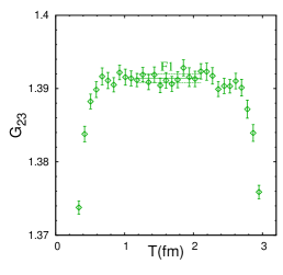
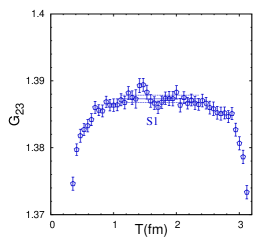
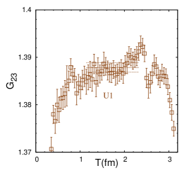
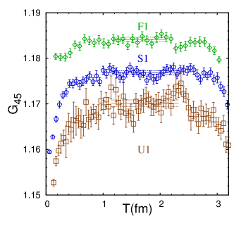
To increase statistics, we do multiple measurements on each configuration. For each measurement, the source position $t_{1}$ is chosen randomly, with $t_{2}$ determined by $t_{2}=t_{1}+\Delta t$, where $\Delta t$ is the wall-source separation listed in Table 4. In addition, we use different random numbers for the wall sources for each measurement. The number of measurements for each gauge configuration is listed in Table 1.

(a) $[P\times P\text{]}[P\times P\text{]}_{I}$

(b) $[P\times P\text{]}[P\times P\text{]}_{II}$

Figure 3: Statistical errors for bare three-point functions as a function of bin size. The operators are (a) $\mathcal{O}_{P1}^{\textrm{Lat}}$, and (b) $\mathcal{O}_{P2}^{\textrm{Lat}}$, respectively, at $T=20$ (F1) and $T=30$ (S1). (Red) circles are the results on F1 ensemble, with $(am_{x},am_{y})=(0.003,0.03)$; and (blue) crosses are the results on S1 ensemble, with $(am_{x},am_{y})=(0.0018,0.018)$.

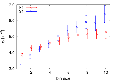
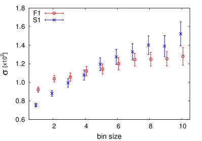
To study auto-correlations we bin adjacent lattices in the Markov chain and study the dependence of the nominal statistical error on bin size. Examples of the results are shown in Fig. 3. The notation for the operators used in this figure is explained in Refs. Kim et al. (2011a, 2014a). We find that the auto-correlations increase as the lattice spacing decreases. As one can see from Fig. 3, the auto-correlation effect is about 100% for the MILC superfine lattice S1, while it is about 25% for the MILC fine lattice F1. In order to greatly reduce the effects of auto-correlations, we use bins of size 5 throughout our analysis.

IV Chiral Extrapolation

Our analysis follows the same steps as in Refs. Bae et al. (2013, 2014). The first step is the chiral extrapolation of the valence quark masses to their physical values. We extrapolate $m_{x}$ to the $m_{d}^{\text{phys}}$ for fixed $m_{y}$ using a fitting form based on SU(2) SChPT, and then extrapolate $m_{y}$ to $m_{s}^{\text{phys}}$. For SU(2) ChPT to be valid, we require that $m_{x}\ll m_{y}$. Hence, from the 10 valence quark masses listed in Eq. (7), we take the lightest four for $m_{x}$ (e.g. $m_{x}=\{0.003,~{}0.006,~{}0.009,~{}0.012\}$ on the fine ensemble) and heaviest three for $m_{y}$ (e.g. $m_{y}=\{0.024,~{}0.027,~{}0.03\}$ on the fine ensemble). In this way we satisfy $m_{x}\leq m_{y}/2$.

We begin by considering the extrapolation in $m_{x}$, which we call the “X fit”. The actual extrapolation is done in $X_{P}=m_{xx,P}^{2}$, which is the squared mass of the $x\bar{x}$ valence pion with taste $\xi_{5}$ (i.e. the Goldstone pion). For the physical value of this quantity we take $X_{P}=2M_{K_{0},\rm phys}^{2}-M_{ss,\rm phys}^{2}=(0.158\;{\rm GeV})^{2}$. At next-to-leading order (NLO) in SU(2) SChPT, the light valence quark mass dependence of the B-parameters has been worked out in Ref. Bailey et al. (2012a), and is

$$B_{i}(\text{NLO})=c_{1}F_{0}(i)+c_{2}X,$$ (9)

where $X\equiv\dfrac{X_{P}}{\Lambda_{\chi}^{2}}$ with $\Lambda_{\chi}=1\mathop{\rm GeV}\nolimits$, the $c_{j}$ are coefficients to be determined, and

$$F_{0}(i) =1\pm\frac{1}{32\pi^{2}f^{2}}\Bigg{\{}\ell(X_{I})+(L_{I}-X_{I})\tilde{\ell}(X_{I})$$

$$\qquad\qquad\qquad\qquad\qquad-\frac{1}{16}\sum_{B}\ell(X_{B})\Bigg{\}}\,,$$ (10)

is the chiral logarithm. Here $X_{B}$ ($L_{B}$) is the squared mass of the taste $B$, flavor non-singlet, pion composed of two light valence (sea) quarks: $X_{B}=m^{2}_{xx,B}$ ($L_{B}=m^{2}_{ll,B}$). The functions $\ell(X)$ and $\tilde{\ell}(X)$ are chiral logarithms defined, for example, in Ref. Bailey et al. (2012a). In Eq. (IV), the plus sign applies for $i=K,2,3$, and the minus sign for $i=4,5$.

The NLO fitting function is not accurate enough to describe the precise and highly correlated data. Hence, as in all our recent analyses Bae et al. (2012, 2013, 2014), we add higher order terms to the fitting function:

$$B_{j}(\text{NNNLO}) =c_{1}F_{0}(j)+c_{2}X+c_{3}X^{2}+c_{4}X^{2}\ln^{2}(X)$$

$$\quad+c_{5}X^{2}\ln(X)+c_{6}X^{3}.$$ (11)

The three terms $X^{2},X^{2}\ln^{2}(X)$ and $X^{2}\ln(X)$ are the generic NNLO terms in continuum chiral perturbation theory. We also add a single analytic NNNLO term proportional to $X^{3}$. We use a similar fitting function for the X fits of gold-plated combinations, except that, by construction, there are no NLO chiral logarithms:

$$G_{i}(\text{NNNLO}) =c_{1}+c_{2}X+c_{3}X^{2}+c_{4}X^{2}\ln^{2}(X)$$

$$\quad+c_{5}X^{2}\ln(X)+c_{6}X^{3}.$$ (12)

We have found that adding yet higher order terms in the chiral expansion does not improve the fits to either the $B_{i}$ or $G_{i}$.

Since we have only four data points for the X fit, we use the Bayesian method Lepage et al. (2002), and place constraints on the three higher-order fitting parameters $c_{4-6}$. Our prior information is that these coefficients are of $\mathcal{O}(1)$. We thus first impose the constraints $c_{4-6}=0\pm 1$. If the resulting fits have $\chi^{2}/{\rm d.o.f.}\lesssim 1$, then we accept them. If not, we try the less restrictive constraints $c_{4-6}=0\pm 2$. Again, we accept fits with $\chi^{2}/{\rm d.o.f.}\lesssim 1$, but otherwise fit again using $c_{4-6}=0\pm 4$. In all cases this leads to fits having $\chi^{2}/{\rm d.o.f.}\lesssim 1$. In this discussion, the $\chi^{2}$ that is minimized is the augmented version:

$$\chi^{2}_{\text{aug}} =\chi^{2}+\chi^{2}_{\text{prior}},$$ (13)

$$\chi^{2}_{\text{prior}} ={\displaystyle\sum_{i=4}^{6}\frac{(c_{i}-a_{i})^{2}}{\sigma_{i}^{2}}}\,,$$ (14)

where we set $a_{i}=0$ and $\sigma_{i}=1,2,4$. These fits are done using the full correlation matrix, and have acceptable values of $\chi^{2}$.

Having determined the parameters $c_{1-6}$, we extrapolate the results to the physical point $m_{x}=m_{d}^{\text{phys}}$, and simultaneously remove (by hand) the lattice artifacts that lead to taste symmetry breaking in pion masses. Specifically, within the chiral logarithm $F_{0}(i)$ we set $X_{B}$ and $L_{I}$ to their physical values, as explained in Ref. Bae et al. (2010). In this way we are using knowledge from SChPT to remove a significant source of discretization errors. Note that this correction applies to the $B_{i}$ but not to the $G_{j}$, since the gold-plated combinations have no chiral logarithms at NLO.

(a) X-fit for $B_{K}$

(b) Y-fit for $B_{K}$

Figure 4: 4(a) X fits and 4(b) Y fits for $B_{K}$ evaluated at $\mu=1/a$ on the F1, S1 and U1 ensembles. The valence strange-quark masses are $am_{y}=0.03$, $0.018$ and $0.014$, respectively. Lattice results are shown with circles (green, blue and brown for F1, S1, and U1, respectively) and are ordered vertically as shown in the legend. Extrapolated results are shown with [green] triangles (F1), [blue] diamonds (S1) and [brown] pentagons (U1). For the X fit, the extrapolated results lie below the curves because of the removal of taste-breaking effects, as described in the text.

(a) X-fit for $G_{23}$

(b) Y-fit for $G_{23}$

Figure 5: 5(a) X fits and 5(b) Y fits for $G_{23}$. Notation as in Fig. 4, except that for the gold-plated combinations there is no taste-breaking correction.

(a) X-fit for $G_{45}$

(b) Y-fit for $G_{45}$

Figure 6: 6(a) X fits and 6(b) Y fits for $G_{45}$. Notation as in Fig. 4.

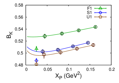
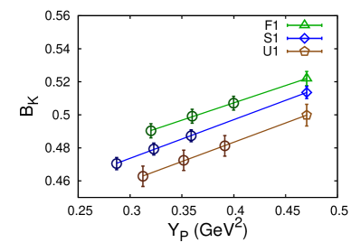
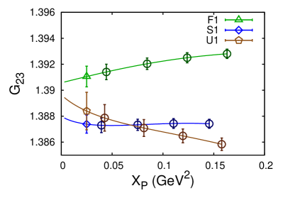
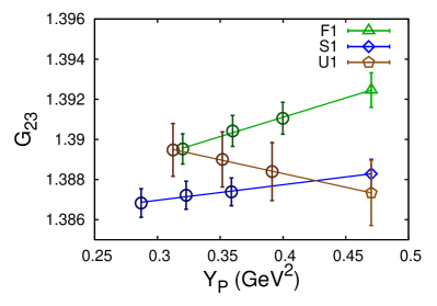
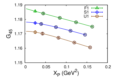
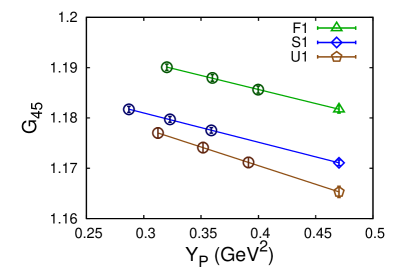
Examples of the X fits are shown in Figs. 44(a), 55(a), and 66(a), for $B_{K}$, $G_{23}$ and $G_{45}$, respectively. In all these fits it was sufficient to use the narrowest range of the Bayesian priors ($\sigma_{i}=1$) in order to obtain good fits. We note that the statistical errors appear larger in the results for $G_{23}$ because of the finer vertical scale. The figures emphasize the fact that the extrapolation in $X_{P}$ is relatively short. Thus the dependence on SChPT is relatively mild, except for the taste-breaking correction that we make to $B_{K}$.

In order to estimate the systematic uncertainty in the X fits we consider two variations in the fitting scheme. The first error is obtained from the changes in the $B_{i}$ and $G_{j}$ when the prior widths $\sigma_{a}$ are doubled. The second is obtained by repeating the fits keeping only one NNLO term,

$$B_{K}(\text{NNLO}) =c_{1}F_{0}(K)+c_{2}X+c_{3}X^{2}\,,$$ (15)

$$G_{i}(\text{NNLO}) =c_{1}+c_{2}X+c_{3}X^{2}\,,$$ (16)

and using the eigenmode shift (ES) method introduced in Ref. Yoon et al. (2013). The ES method tunes the fitting function in the direction of the eigenvectors of the covariance matrix corresponding to the small eigenvalues, with small shifting parameters $\eta$ that are constrained by the Bayesian prior condition: $\eta=0\pm\sigma_{\eta}$. We set $\sigma_{\eta}$ from the size of the neglected highest order term in the fitting function,

$$\sigma_{\eta}=0.006\approx X^{2}(\ln(X))^{2},$$ (17)

where $X\approx 0.02$.

The total systematic error from the X fits is then obtained by adding these two error estimates in quadrature. The resulting errors are discussed in Sec. VI.

We next extrapolate $m_{y}$ to $m_{s}^{\rm phys}$, using the three heaviest values of the valence quark masses. This we denote the “Y fit”. We expect the $B_{i}$ and $G_{j}$ to be smooth, analytic functions of $Y_{P}$, since the strange quark is far from the chiral limit. Empirically, linear fitting works very well, as illustrated in Figs. 44(b), 55(b) and 66(b). To avoid the problem of small eigenvalues, we use uncorrelated fitting for the Y fits. In all cases, fits are stable and the fit parameters are consistent across all lattices with a given nominal lattice spacing (within the statistical uncertainties). To estimate the systematic error in the results of the Y fits, we repeat the fits using a quadratic function of $Y_{P}$. The changes in the final results for $B_{i}$ and $G_{j}$ are then taken as the systematic error.

V Continuum-chiral extrapolation

The outputs of the extrapolations in valence masses are values for the $B$-parameters and gold-plated combinations on each ensemble, for continuum operators evaluated at the renormalization scale $\mu=1/a$. In order to compare these results and extrapolate them to the continuum limit, and to physical sea-quark masses, we must use renormalization group (RG) evolution to evolve to a common scale. The standard choices for this scale in the literature are $\mu=2\;\mathop{\rm GeV}\nolimits$ and $\mu=3\;\mathop{\rm GeV}\nolimits$, and we present results for both. Since we use one-loop matching, to do the running consistently we need the continuum two-loop anomalous dimension matrix. This has been calculated in Ref. Buras et al. (2000) for a particular choice of evanescent operators. Because of this, it is essential that our lattice-continuum matching uses the same set of evanescent operators, as is indeed the case in Ref. Kim et al. (2014a). Some technical issues arise in the RG running; these are described in Ref. Kim et al. (2014a) along with our resolutions.

We present our results for $B_{K}$ and the gold-plated combinations $G_{i}$ at the two renormalization scales in Tables 5 and 6. Statistical errors range from the percent level to an order of magnitude smaller. We have also obtained results for the $B_{j}$ ($j=2-5$) but do not show these as they are not used in our final analysis.

Table 5: $B_{K}$ and gold-plated combinations for $\mu=2\mathop{\rm GeV}\nolimits$ on each lattice listed in Table 1. The superscripts indicate whether broadened Bayesian priors have been used in the X-fits: $\dagger$ implying $c_{4-6}=0\pm 2$, while $\ddagger$ implying $c_{4-6}=0\pm 4$. Results without superscripts are obtained with $c_{4-6}=0\pm 1$.

ID	$B_{K}$	$G_{21}$	$G_{23}$	$G_{24}$	$G_{45}$
C1	0.5484(55)	$0.995(11)^{\dagger}$	1.4140(10)	0.6205(19)	1.1836(7)
C2	0.5528(56)	$0.993(11)^{\dagger}$	1.4119(11)	0.6232(22)	1.1824(8)
C3	0.5673(52)	$0.975(10)^{\ddagger}$	1.4098(9)	0.6256(20)	1.1819(7)
C3-2	0.5715(51)	$0.974(9)^{\dagger}$	1.4105(9)	0.6229(16)	1.1823(6)
C4	0.5641(54)	$0.987(11)^{\ddagger}$	1.4113(9)	0.6291(19)	1.1822(6)
C5	0.5677(46)	$0.976(8)^{\dagger}$	1.4082(8)	0.6264(15)	1.1834(5)
F1	0.5294(43)	1.0451(69)	1.4000(10)	0.6092(19)	1.2003(9)
F2	0.5451(35)	1.0281(59)	1.3985(6)	0.6088(11)	1.1993(5)
F3	0.5226(49)	$1.053(10)^{\dagger}$	1.4015(11)	0.6119(21)	1.1991(10)
F4	0.5255(30)	$1.0366(64)^{\ddagger}$	1.4033(7)	0.6050(12)	1.2008(6)
F5	0.5388(43)	$1.0322(84)^{\dagger}$	1.3995(9)	0.6101(17)	1.1997(8)
F6	$0.5472(59)^{\dagger}$	$1.014(11)^{\ddagger}$	1.3991(13)	0.6123(23)	1.2018(9)
F7	0.5392(35)	1.0394(59)	1.3953(7)	0.6130(12)	1.1992(6)
F9	0.5501(16)	1.0258(30)	1.3976(3)	0.6093(6)	1.1991(3)
S1	0.5359(38)	1.0531(55)	1.4140(10)	0.5858(17)	1.2288(8)
S2	0.5361(36)	1.0423(57)	1.4116(9)	0.5833(13)	1.2278(8)
S3	$0.5261(41)^{\dagger}$	$1.0625(79)^{\ddagger}$	1.4184(13)	0.5842(20)	1.2278(10)
S4	0.5204(33)	1.0621(60)	1.4124(10)	0.5820(18)	1.2277(8)
S5	0.5384(36)	1.0446(55)	1.4110(8)	0.5835(12)	1.2287(8)
U1	0.5325(70)	1.056(11)	1.4302(28)	0.5718(39)	1.2539(19)

Table 6: $B_{K}$ and gold-plated combinations for $\mu=3\mathop{\rm GeV}\nolimits$ on each lattice listed in Table 1. The convention for $\dagger$ and $\ddagger$ is the same as Table 5.

ID	$B_{K}$	$G_{21}$	$G_{23}$	$G_{24}$	$G_{45}$
C1	0.5298(53)	$0.951(10)^{\dagger}$	1.3942(8)	0.5713(18)	1.1468(6)
C2	0.5341(54)	$0.950(10)^{\dagger}$	1.3926(8)	0.5738(20)	1.1459(6)
C3	0.5481(50)	$0.9323(97)^{\ddagger}$	1.3911(7)	0.5760(19)	1.1455(5)
C3-2	0.5521(49)	$0.9308(89)^{\dagger}$	1.3915(7)	0.5735(14)	1.1458(5)
C4	0.5449(52)	$0.944(10)^{\ddagger}$	1.3921(7)	0.5792(18)	1.1457(5)
C5	0.5484(45)	$0.9327(80)^{\dagger}$	1.3898(6)	0.5767(14)	1.1467(4)
F1	0.5115(42)	0.9991(66)	1.3829(7)	0.5610(18)	1.1594(7)
F2	0.5266(34)	0.9828(56)	1.3817(5)	0.5606(10)	1.1586(4)
F3	0.5049(47)	$1.0069(96)^{\dagger}$	1.3840(9)	0.5634(19)	1.1584(8)
F4	0.5077(29)	$0.9909(61)^{\ddagger}$	1.3853(5)	0.5571(11)	1.1597(4)
F5	0.5205(42)	$0.9867(80)^{\dagger}$	1.3825(6)	0.5618(16)	1.1589(6)
F6	$0.5287(57)^{\dagger}$	$0.969(10)^{\ddagger}$	1.3821(10)	0.5639(21)	1.1604(7)
F7	0.5210(34)	0.9935(56)	1.3793(5)	0.5645(11)	1.1585(5)
F9	0.5314(16)	0.9806(29)	1.3811(3)	0.5611(5)	1.1585(2)
S1	0.5178(37)	1.0068(53)	1.3927(8)	0.5394(16)	1.1806(6)
S2	0.5179(34)	0.9965(55)	1.3909(7)	0.5372(12)	1.1798(6)
S3	$0.5083(39)^{\dagger}$	$1.0158(76)^{\ddagger}$	1.3960(10)	0.5380(19)	1.1798(8)
S4	0.5028(31)	1.0153(58)	1.3916(8)	0.5359(16)	1.1797(6)
S5	0.5202(34)	0.9986(53)	1.3905(6)	0.5373(12)	1.1805(6)
U1	0.5145(67)	1.009(10)	1.4044(21)	0.5266(36)	1.1991(14)

The final step of our analysis is to do a simultaneous extrapolation to the physical values of the sea-quark masses and to the continuum limit. We call this procedure “the continuum-chiral extrapolation”, although this name is slightly misleading as the valence chiral extrapolation has already been done. As substitutes for sea quark masses, we use $L_{P}$ and $S_{P}$, which are, respectively, the squared masses of taste-$\xi_{5}$ (Goldstone) pions composed of two light sea quarks ($l\bar{l}$) and two strange sea quarks ($s\bar{s}$). They are extrapolated to their physical values, which we take to be $m_{\pi_{0}}^{2}=(0.1349766\mathop{\rm GeV}\nolimits)^{2}$ for $L_{P}$ and $M_{ss,\rm phys}^{2}=(0.6858\mathop{\rm GeV}\nolimits)^{2}$ for $S_{P}$ Davies et al. (2010).

We expect the dependence of the $B_{i}$ and $G_{j}$ on $L_{P}$, $S_{P}$ and $a^{2}$ to be analytic, with terms organized according to standard SChPT power counting. At NLO, the only term in SChPT that could violate this expectation is the chiral logarithm. This is absent for the $G_{j}$. For the $B_{i}$, as shown by Eq. (IV), the only logarithms that appear have the schematic dependence $(L_{P}+a^{2})\log X_{B}$ and $X_{B}\log X_{B}$. Since $X_{B}$ is set by hand to its physical value, the $a^{2}$ dependence it contains is removed. The remaining dependence on $L_{P}$ and $a^{2}$ is analytic, and in fact also is removed by hand when we set $L_{P}$ to its physical value and $a^{2}$ to zero. Chiral logarithms of higher order can lead to non-analyticities, or large derivatives, but these are numerically suppressed. Thus, to good approximation, we expect all the quantities we calculate to be described by

$$\tilde{F}_{1}=d_{1}+d_{2}\frac{L_{P}}{\Lambda_{\chi}^{2}}+d_{3}\frac{S_{P}-M_{ss,\rm phys}^{2}}{\Lambda_{\chi}^{2}}+d_{4}(a\Lambda_{Q})^{2}\,.$$ (18)

Here $\Lambda_{Q}=0.3\;$GeV and $\Lambda_{\chi}=1\;$GeV, and we have chosen to expand the $d_{3}$ term about the physical $s\bar{s}$ mass.

When we fit our results to this form, we impose Bayesian constraints on the linear terms to enforce the expected power counting: $d_{2-4}=0\pm 2$. We have also tried fits with broader contraints, $d_{2-4}=0\pm 4$, but find that these do not significantly change the $\chi^{2}$ or the resulting fit parameters. We find, as was the case in our earlier work Bae et al. (2012, 2013, 2014) that we cannot obtain a good description if we include the coarse lattices. Thus we fit all the fine, superfine and ultrafine lattice data to Eq. (18). We call this the $\tilde{F}_{1}$ fit, since it is a small variation from the fitting function $F^{1}_{B}$ in our previous work Bae et al. (2014) (differing only in the offset in the $d_{3}$ term). Since the number of configurations differ on each ensemble, errors on the fit parameters are obtained using a variant of the bootstrap method. Note that for this fit there are no correlations between the different ensembles.

Table 7: Results of $\tilde{F}_{1}$ fits to $B_{K}$ and the gold-plated combinations. The renormalization scale is $\mu=2\mathop{\rm GeV}\nolimits$.

	$B_{K}$	$G_{21}$	$G_{23}$	$G_{24}$	$G_{45}$
$d_{1}$	0.5390(37)	1.0568(62)	1.4248(10)	0.5590(15)	1.2567(8)
$d_{2}$	-0.127(14)	0.095(27)	0.0275(33)	-0.0097(56)	0.0041(26)
$d_{3}$	0.006(15)	-0.014(25)	0.0145(30)	-0.0207(53)	0.0026(25)
$d_{4}$	0.78(25)	-1.92(41)	-1.799(64)	3.21(10)	-3.529(53)
$B_{K}$ or $G_{i}$	0.5366(36)	1.0585(59)	1.4253(10)	0.5589(15)	1.2568(8)
$\chi^{2}/\text{dof}$	1.53	1.30	2.01	1.08	4.07

(a) $\tilde{F}_{1}$: $\chi^{2}/\text{d.o.f}=1.53$

(b) $\tilde{F}_{4}$: $\chi^{2}/\text{d.o.f}=1.52$

Figure 7: Continuum-chiral extrapolation for $B_{K}$ renormalized at $\mu=2\mathop{\rm GeV}\nolimits$. Results from the fine, superfine and ultrafine lattices are shown with (green) triangles, (blue) diamonds and the (brown) pentagon, respectively. (a) $\tilde{F}_{1}$ fit; (b) $\tilde{F}_{4}$ fit. The (red) circle gives the extrapolated result. Due to the variations in values of $S_{P}$ and $a$, the curves should not pass precisely through all the points. For more discussion, see text.

(a) $\tilde{F}_{1}$: $\chi^{2}/\text{d.o.f}=1.30$

(b) $\tilde{F}_{4}$: $\chi^{2}/\text{d.o.f}=1.23$

Figure 8: Continuum-chiral extrapolation results for $G_{21}$ at $\mu=2\mathop{\rm GeV}\nolimits$. The notation is as in Fig. 7.

(a) $\tilde{F}_{1}$: $\chi^{2}/\text{d.o.f}=2.01$

(b) $\tilde{F}_{4}$: $\chi^{2}/\text{d.o.f}=1.33$

Figure 9: Continuum-chiral extrapolation results for $G_{23}$ at $\mu=2\mathop{\rm GeV}\nolimits$. The notation is as in Fig. 7.

(a) $\tilde{F}_{1}$: $\chi^{2}/\text{d.o.f}=1.08$

(b) $\tilde{F}_{4}$: $\chi^{2}/\text{d.o.f}=0.91$

Figure 10: Continuum-chiral extrapolation results for $G_{24}$ at $\mu=2\mathop{\rm GeV}\nolimits$. The notation is as in Fig. 7.

(a) $\tilde{F}_{1}$: $\chi^{2}/\text{d.o.f}=4.07$

(b) $\tilde{F}_{4}$: $\chi^{2}/\text{d.o.f}=1.39$

Figure 11: Continuum-chiral extrapolation results for $G_{45}$ at $\mu=2\mathop{\rm GeV}\nolimits$. The notation is as in Fig. 7.

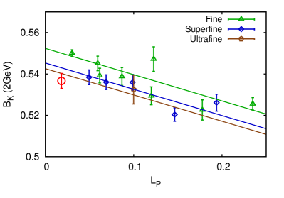
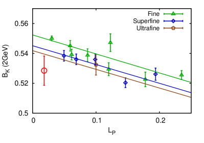
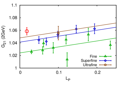
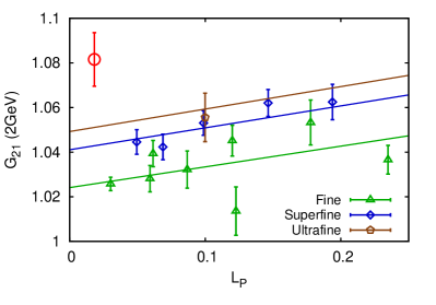
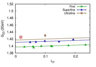
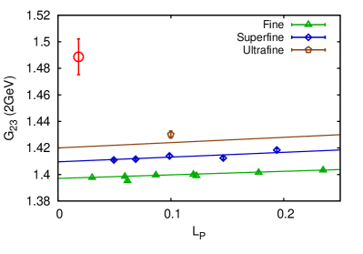
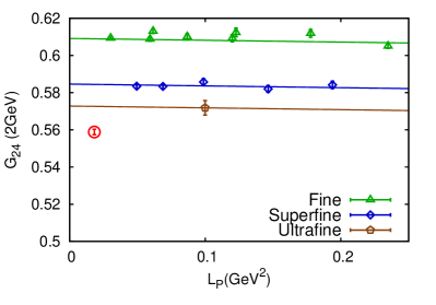
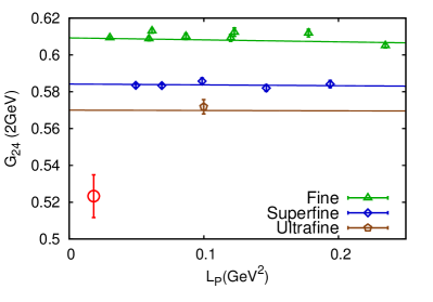
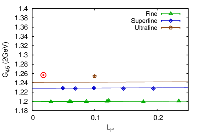
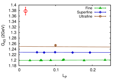
In Table 7, we show the results of the $\tilde{F}_{1}$ fits to $B_{K}$ and the $G_{i}$ (renormalized at $\mu=2\mathop{\rm GeV}\nolimits$). Plots of the fits are shown in Figs. 77(a), 88(a), 99(a), 1010(a), and 1111(a). The fits are qualitatively similar and of comparable quality if the operators are renormalized at $\mu=3\mathop{\rm GeV}\nolimits$. To interpret these plots the following must be kept in mind. For each nominal value of $a$ (e.g. for the fine lattices) there is a variation in the actual values of $a$ and in the values of $S_{P}$. This is most significant for the ensembles F6 and F7, which have a substantially lower strange quark mass than the other fine ensembles. These variations are accounted for in the fit (with F6 and F7 providing a significant lever arm to determine $d_{3}$), but do not show up in these two-dimensional plots. Indeed, the points from F6 and F7 are not included in the plots, while the fit lines for the fine and superfine ensembles are shown with $a$ and $S_{P}$ set to their average values (excluding ensembles F6 and F7 for the fine lattices). Thus, even if the fit were perfect, the fit lines would not pass through any of the points, except for the ultrafine case. Because of this, the fits appear slightly worse than they actually are; the real indicator of goodness of each fit is the quoted value of $\chi^{2}/\text{d.o.f.}$.

The fits indicate that the dependence on the strange sea-quark mass is very weak for all five quantities, with $|d_{3}|\ll 1$. For the gold-plated combinations, the dependence on the light sea-quark mass is also weak, much weaker within our range of parameters than the dependence on $a$. Only for $B_{K}$ does the variation with $L_{P}$ have a similar magnitude to that with $a$. The values of the $a^{2}$ coefficient, $d_{4}$, indicate that scale describing $a^{2}$ effects ranges from $\sim 0.3\;$GeV ($|d_{4}|\sim 1$) up to $\sim 0.55\;$GeV ($|d_{4}|\sim 3.5$). These scales are not unusual for discretization errors with improved staggered fermions. The $\chi^{2}/\text{d.o.f.}$ of these fits is reasonable for $B_{K}$, $G_{21}$, and $G_{24}$. Hence, we choose the results from the $\tilde{F}_{1}$ fits for our central values for these quantities. However, we cannot use the $\tilde{F}_{1}$ results for $G_{23}$ and $G_{45}$, since the fit quality is too poor. This is primarily due to the difficulty that the fits have in reproducing the dependence on $a$.

Table 8: Fit results for BSM B-parameters and the gold-plated combinations obtained using $\tilde{F}_{4}$-fit at $\mu=2\mathop{\rm GeV}\nolimits$.

	$B_{K}$	$G_{21}$	$G_{23}$	$G_{24}$	$G_{45}$
$d_{1}$	0.5308(99)	1.080(12)	1.488(14)	0.523(12)	1.378(14)
$d_{2}$	-0.124(18)	0.104(28)	0.045(14)	0.001(16)	-0.013(12)
$d_{3}$	0.005(15)	-0.011(25)	0.019(6)	-0.021(6)	0.012(7)
$d_{4}$	0.24(40)	-0.33(27)	2.22(75)	0.84(63)	3.70(80)
$d_{5}$	-0.18(77)	-0.66(48)	-1.10(87)	-0.7(10)	1.16(78)
$d_{6}$	0.10(10)	-0.081(63)	-0.29(34)	0.03(22)	-0.64(42)
$d_{7}$	0.09(21)	-0.10(14)	1.20(40)	0.33(33)	2.06(42)
$d_{8}$	0.22(21)	-0.65(20)	-1.80(37)	0.98(31)	-3.34(39)
$d_{9}$	0.008(31)	-0.008(21)	0.183(60)	0.036(50)	0.322(64)
$B_{K}$ or $G_{i}$	0.5285(98)	1.082(12)	1.489(13)	0.523(12)	1.378(14)
$\chi^{2}/\text{dof}$	1.52	1.23	1.33	0.91	1.39

To obtain reasonable fits for $G_{23}$ and $G_{45}$, we add higher order terms to the fitting function, denoting the new form $\tilde{F}_{4}$:

$$\tilde{F}_{4}=\tilde{F}_{1} +d_{5}(a\Lambda_{Q})^{2}\frac{L_{P}}{\Lambda^{2}_{\chi}}+d_{6}(a\Lambda_{Q})^{2}[\frac{S_{P}-m_{s\bar{s}}^{2}}{\Lambda^{2}_{\chi}}]$$

$$+d_{7}(a\Lambda_{Q})^{2}\alpha_{s}+d_{8}\alpha_{s}^{2}+d_{9}(a\Lambda_{Q})^{4}$$ (19)

where $\alpha_{s}=\alpha_{s}^{\overline{\text{MS}}}(1/a)$. In other words, we add a subset of the analytic terms quadratic in $L_{P}$, $S_{P}$ and $a^{2}$, as well as two terms that include logarithmic dependence on $a$. The $d_{7}$ term would be the dominant source of $a$ dependence were the action and operators tree-level ${\cal O}(a^{2})$ improved. In fact, our valence fermion action and operators are not tree-level improved, so we must include the pure $a^{2}$ $d_{4}$ term as well. Nevertheless, we expect the tree-level contributions proportional to $a^{2}$ alone to be small, due to the use of HYP-smeared gauge fields. The $d_{8}$ term arises because our lattice operators are only matched to the continuum operators at one-loop order, leaving a two-loop residual discrepancy. In the $\tilde{F}_{4}$ fits we constrain $d_{2-9}$ using the Bayesian method, choosing the prior conditions $d_{2-9}=0\pm 2$. Again we find that broadening the priors does not significantly improve the fits.

The results for the $\tilde{F}_{4}$ fits are shown (for $\mu=2\mathop{\rm GeV}\nolimits$) in Table 8 and Figs. 77(b), 88(b), 99(b), 1010(b), and 1111(b). With the additional terms, we obtain reasonable values of $\chi^{2}/\text{d.o.f}$ for $G_{23}$ and $G_{45}$, and we take the resulting extrapolated values as our final results for these two quantities. For the other quantities, the fit quality is only slightly improved.

As is apparent, particularly from Figs. 99(b), 1010(b) and 1111(b), the change from $\tilde{F}_{1}$ to $\tilde{F}_{4}$ fits has a very significant impact on the continuum extrapolation. This is primarily due to the $d_{8}\alpha_{S}^{2}$ term, which has a rapid dependence on $a$ as $a\to 0$. We note that the coefficients of this term in the fits to $G_{23}$ and $G_{45}$ are relatively large [although still of ${\cal O}(1)$], and this is what leads to the large change in the extrapolated value between the fits. We do not find the $\tilde{F}_{4}$ fits to provide a convincing description of the $a$ dependence, particularly as they depend very strongly on the result from the single ultrafine lattice. However, we think that the conservative choice is to use the better fit for the central value, and then to take the difference between the two fits as an estimate of the systematic error in the continuum-chiral extrapolation. The final results from the two fits, and the resulting estimate of the systematic error, are collected in Table 9. For $G_{23}$, $G_{24}$ and $G_{45}$ this source of error dominates all others, as discussed in the following section.

We have also used fit functions with additional higher-order terms. These do lead to mild reductions in the values of $\chi^{2}/\text{d.o.f}$, but do not lead to significant changes in the central values compared to the $\tilde{F}_{4}$ fits. Thus they do not significantly change our estimates of systematic errors. For the sake of brevity, we do not display the results of these more elaborate fits.

Table 9: Results for $B_{K}$ and $G_{i}$ (renormalized at $\mu=2\mathop{\rm GeV}\nolimits$) from continuum-chiral extrapolation using the $\tilde{F}_{1}$ and $\tilde{F}_{4}$ fits. Our choices for the final central values are (red and) underlined. $\Delta$ is the fractional systematic error in the continuum-chiral extrapolation, and is obtained from the difference between the two fits.

	$\tilde{F}_{1}$	$\tilde{F}_{4}$	$\Delta(\%)$
$B_{K}$	0.5366(36)	0.5285(98)	1.52
$G_{21}$	1.0585(59)	1.082(12)	2.18
$G_{23}$	1.4253(10)	1.489(13)	4.26
$G_{24}$	0.5589(15)	0.523(12)	6.36
$G_{45}$	1.2568(8)	1.378(14)	8.79

We close this section by returning to the option of directly fitting the BSM $B$-parameters rather than using the gold-plated combinations. In all cases we find that direct continuum-chiral fits have values of $\chi^{2}/\text{d.o.f.}$ in the range $3-5$, both for $\tilde{F}_{1}$ and $\tilde{F}_{4}$ (and more elaborate) fits. We do not fully understand this failure of the continuum-chiral fits, but suspect that it is related to errors in valence chiral extrapolation (X fits). The X fits are better controlled with the gold-plated combinations.

VI Final Results and Error Budget

In this section we discuss all sources of error, and give our final results for the BSM $B$-parameters with their error budget. Because we obtain $B^{G}_{2-5}$ using Eq. (6), we estimate the errors in $B_{K}$ and the $G_{i}$ first, and then propagate the errors to $B^{G}_{2-5}$. Our final results for the two standard renormalization scales are given in Tables 10 and 11, while the final error budget is given in Table 12. 

Table 10: Final results for $B_{K}$ and the BSM $B$-parameters at renormalization scales $\mu=2\mathop{\rm GeV}\nolimits$ and $\mu=3\mathop{\rm GeV}\nolimits$. The first error is statistical, the second systematic.

	$\mu=2\mathop{\rm GeV}\nolimits$	$\mu=3\mathop{\rm GeV}\nolimits$
$B_{K}$	0.537(4)(26)	0.519(4)(26)
$B^{G}_{2}$	0.568(1)(25)	0.525(1)(23)
$B^{G}_{3}$	0.382(4)(17)	0.360(4)(16)
$B^{G}_{4}$	0.984(3)(64)	0.981(3)(62)
$B^{G}_{5}$	0.714(7)(71)	0.751(7)(68)

Table 11: Final results for the gold-plated combinations $G_{i}$. Notation as in Table 10.

	$\mu=2\mathop{\rm GeV}\nolimits$	$\mu=3\mathop{\rm GeV}\nolimits$
$G_{21}$	1.059(6)(52)	1.012(6)(50)
$G_{23}$	1.489(13)(66)	1.460(14)(65)
$G_{24}$	0.559(1)(36)	0.515(1)(32)
$G_{45}$	1.378(14)(123)	1.307(14)(107)

Table 12: Error budget for the $B_{i}$ and $G_{j}$ evaluated at renormalization scale $\mu=2\mathop{\rm GeV}\nolimits$. All entries are in percent.

cause	$B_{K}$	$G_{21}$	$G_{23}$	$G_{24}$	$G_{45}$	$B^{G}_{2}$	$B^{G}_{3}$	$B^{G}_{4}$	$B^{G}_{5}$	$B_{3}^{G,\text{SUSY}}$	method
statistics	0.67	0.56	0.87	0.27	1.02	0.25	1.00	0.27	0.98	0.66	see text
$\left\{\begin{array}[]{l}\text{matching}\\ \text{cont-extrap.}\end{array}\right\}$	4.40	4.40	4.40	6.36	8.79	4.40	4.45	6.36	9.63	4.40	($\tilde{F}_{1}$ vs. $\tilde{F}_{4}$) or $\alpha_{s}^{2}$ (U1)
finite volume	0.73	0.17	0.05	0.43	0.04	0.56	0.52	0.99	1.02	0.60	(C3) vs. (C3-2)
X-fits	0.05	0.40	0.45	0.02	0.96	0.36	0.34	0.37	1.23	0.60	change Bayes. prior & fit method
Y-fits	2.07	2.11	0.32	0.48	1.12	0.00	0.32	0.48	1.59	0.22	linear vs. quad.
$f_{\pi}$	0.10	0	0	0	0	0.10	0.10	0.10	0.10	0.10	$132\;$MeV vs. $124.2\;$MeV.
$r_{1}$	0.35	0.28	0.11	0.16	0.21	0.07	0.17	0.09	0.30	0.01	errors due to $r_{1}$ ambiguity.
Total	4.93	4.91	4.44	6.39	8.92	4.45	4.51	6.47	9.90	4.49

As can be seen from Table 12, the statistical errors in $B_{K}$ and the $G_{i}$ are small, ranging from $\sim 0.25\%$ to $\sim 1\%$. The largest are those in $G_{23}$ and $G_{45}$, resulting from the use of the $\tilde{F}_{4}$ fits for the continuum-chiral extrapolation. We propagate the statistical errors into the $B^{G}_{j}$ using the bootstrap method. The larger errors in $G_{23}$ and $G_{45}$ then lead to $B^{G}_{3}$ and $B^{G}_{5}$ having the largest statistical errors of the BSM $B$-parameters. In all cases, however, the statistical errors are much smaller than those from systematic effects.

We now run through the systematic errors in the order listed in Table 12. The dominant error is that due to the combined effect of using one-loop matching and the continuum-chiral extrapolation. We combine these because the $\tilde{F}_{4}$ fit includes the $\alpha_{s}^{2}$ error that results from perturbative truncation, and indeed this is the dominant contribution to the systematic error estimate, as discussed above. However, one can also estimate the truncation error directly, following Ref. Bae et al. (2012), by the size of a typical two-loop contribution:

$$\Delta B_{i}\approx B_{i}\times\alpha_{s}^{2}\,.$$ (20)

Here we use $\alpha_{s}$ in the $\overline{\mathrm{MS}}$ scheme evaluated at a scale $1/a_{\rm min}$, where $a_{\rm min}$ is our smallest lattice spacing. This leads to a 4.4% relative error. To avoid double-counting, we take the larger of (a) the direct estimate of two-loop effects (4.4%) and (b) the difference between $\tilde{F}_{1}$ and $\tilde{F}_{4}$ fits. In essence this method is using the $\tilde{F}_{4}$ fit to give an estimate of the uncertainty in the coefficient of the $\alpha_{s}^{2}$ term, except that we do not allow this uncertainty to drop below unity.

The above description applies to quantities we calculate directly, namely $B_{K}$ and the $G_{i}$. For the derived quantities $B^{G}_{j}$, defined in Eq. (6), we proceed as follows. We vary the fit choices (for the continuum-chiral extrapolation) for each of the components of the $B^{G}_{j}$ independently, and take the largest variation from the central value as the systematic error estimate. If this maximum value lies below 4.4%, we replace the estimate with the direct two-loop estimate of a 4.4% error.

We next consider the error due to the finite volume (FV) of the lattice. We estimate this from the difference between results on the C3 and C3-2 ensembles, which differ only in their spatial volumes. This is not entirely satisfactory, since we do not use coarse lattices in our final continuum-chiral extrapolation. However, we stress that the dominant FV error, as estimated by SChPT, comes from valence pions propagating to adjacent periodic volumes. This is because the arguments of the chiral logarithms of Eq. (IV) are the squared masses of valence pions, $X_{B}$. Since on each ensemble we are extrapolating to the physical valence quark masses, the dominant FV effects are present, even though on ensembles C3 and C3-2 we are far from the physical values of $L_{P}$ and $a$. In our calculation of $B_{K}$, we have used the comparison of doing the X-fits with finite- and infinite-volume SChPT forms as an alternative estimate of the FV error Kim et al. (2011b). However, this method is not useful for the gold-plated combinations, since they do not contain NLO chiral logarithms.

Our method of estimating systematic errors arising from the X fits has been described in Sec. IV. We repeat the entire analysis using different priors for the X-fits, and using the ES method. Each leads to a change in the final values of the quantities of interest. We combine the fractional shifts in quadrature to obtain our total systematic error.

Our method of estimating the systematic error arising from Y fits, as noted above, is to repeat the entire analysis (including the continuum-chiral extrapolation) using quadratic, as apposed to linear, functional forms. This differs slightly from the estimate we used in Ref. Bae et al. (2014), where we used the shift in the quantities on a specific MILC ensemble. The Y fit errors turn out to be of comparable size to those from X fits, ranging up to 2%.

The remaining two systematic errors are very small, and have essentially no impact on the total error. We include them for completeness. The first concerns the value of the pion decay constant $f$ that we use in the chiral logarithms of Eq. (IV). At NLO we could equally well use the physical value $f_{\pi}=130.41\mathop{\rm MeV}\nolimits$ Beringer et al. (2012) or the value in the chiral limit, $f_{\pi}\approx 124.2\mathop{\rm MeV}\nolimits$ Bazavov et al. (2010). In practice we use $f=132\mathop{\rm MeV}\nolimits$ (close to the physical value) for our central value, and repeat the entire analysis using $f=124.2\mathop{\rm MeV}\nolimits$ (the chiral-limit value) to estimate the systematic error. In fact, only $B_{K}$ is sensitive to this choice, since the gold-plated combinations contain no NLO chiral logarithms. Thus the 0.1% error that results in $B_{K}$ propagates unchanged into all of the BSM $B$-parameters.

Finally, the parameter we use to set the scale, $r_{1}$, has an error which propagates into all the final results. To estimate this, we repeat the entire analysis with the central value for $r_{1}$ replaced by $r_{1}\pm\sigma_{r_{1}}$, and quote the maximum difference in each quantity as the systematic error. The resulting errors are very small ($\sim 0.1-0.35\%$), reflecting the fact that the $B$-parameters are dimensionless.

VII Comparisons and Outlook

Table 13: Comparison of the BSM $B$-parameters at renormalization scale $\mu=3\mathop{\rm GeV}\nolimits$ obtained using different fermion discretizations. The RBC-UKQCD results using domain-wall fermions are RBC-UK (2012) Boyle et al. (2012) and the preliminary results (with incomplete error budget) of RBC-UK (2015) Hudspith et al. (2015). The ETM collaboration results using twisted-mass fermions are ETM (2012) Bertone et al. (2013) and ETM (2015) Carrasco et al. (2015). N.A. means “not available”.

	SWME (this work)	RBC-UK (2012)	RBC-UK (2015)	ETM (2012)	ETM (2015)
$B_{K}$	0.519(4)(26)	0.53(2)	0.53(1)	0.51(2)	0.51(2)
$B_{2}$	0.525(1)(23)	0.43(5)	0.49(2)	0.47(2)	0.46(3)
$B_{3}^{\text{SUSY}}$	0.773(6)(35)	0.75(9)	0.74(7)	0.78(4)	0.79(5)
$B_{3}^{\text{Buras}}$	0.360(4)(16)	N.A.	N.A.	N.A.	N.A.
$B_{4}$	0.981(3)(62)	0.69(7)	0.92(2)	0.75(3)	0.78(5)
$B_{5}$	0.751(7)(68)	0.47(6)	0.71(4)	0.60(3)	0.49(4)

In Table 13 and Fig. 12 we compare our results for the B-parameters to those from other collaborations. This is done at $\mu=3\mathop{\rm GeV}\nolimits$ since results from all collaborations are available at this choice of renormalization scale. The RBC-UKQCD collaboration uses $N_{f}=2+1$ light flavors of domain wall quarks, and NPR for the matching between lattice and continuum theories. In 2012, RBC-UKQCD used the RI-MOM scheme for this matching Boyle et al. (2012), while the preliminary 2015 results are obtained using several RI-SMOM schemes, in the spirit of Ref. Sturm et al. (2009). Both schemes are connected to the $\overline{\mathrm{MS}}$ scheme using one-loop perturbation theory. The ETM collaboration uses twisted-mass Wilson quarks. The original results from 2012 were with $N_{f}=2$ light sea quarks and a quenched valence strange quark Bertone et al. (2013), while the 2015 results are from an $N_{f}=2+1+1$ simulation including both strange and charmed sea quarks Carrasco et al. (2015). Both ETM calculations match lattice and continuum operators using NPR in the RI-MOM scheme.

Both RBC-UKQCD and ETM results are quoted using the so-called SUSY basis of BSM four-fermion operators Gabbiani et al. (1996). The only BSM $B$-parameter which differs from that in the basis of Buras et al. (Ref. Buras et al. (2000)) that we use is $B_{3}$,

$$\begin{split}B_{3}^{\text{SUSY}}&=-\frac{3}{2}B_{3}^{\text{Buras}}+\frac{5}{2}B_{2}^{\text{Buras}}\,.\end{split}$$ (21)

We use this equation to determine our result for $B_{3}^{\text{SUSY}}$ quoted in Table 13.

For completeness, we note that our 2013 results for the BSM $B$-parameters (Ref. Bae et al. (2013)) are superseded and corrected by our present results. We now have significantly more ensembles, allowing a better controlled continuum-chiral extrapolation. This addition required us to change from $\tilde{F}_{1}$ fits to $\tilde{F}_{4}$ fits for $G_{23}$ and $G_{45}$, which, as shown above, significantly changes the central values for these quantities. In addition, we found an error in our RG running due to the use of an incorrect two-loop contribution to the pseudoscalar anomalous dimension [needed for the denominators of the BSM $B$-parameters—see Eq. (3)]. Correcting this error leads to $\sim 5\%$ reductions in all the BSM $B$-parameters. A detailed description of the effect of these changes is given in Ref. Leem et al. (2014). The overall effect is that our new results for $B_{2}$, $B_{3}^{\text{SUSY}}$, $B_{4}$ and $B_{5}$ are reduced by about 5%, 3%, 5% and 12%, respectively, compared to those in Ref. Bae et al. (2013).

Table 13 shows that the results for $B_{K}$, $B_{2}$ and $B_{3}^{\text{SUSY}}$ are consistent across all calculations, with all results having comparable errors. By contrast, there are significant differences for $B_{4}$ and $B_{5}$, as one can see most clearly from Fig. 12. The preliminary results from RBC-UKQCD (2015) using the intermediate RI-SMOM schemes are consistent with our results, while those using the intermediate RI-MOM scheme [RBC-UK (2012), ETM (2012) and ETM (2015)] differ significantly. For example, the ETM (2015) results for $B_{4}$ and $B_{5}$ differ from our results by $2.6\sigma$ and $3.2\sigma$, respectively.

(a) $B_{4}(3\mathop{\rm GeV}\nolimits)$

(b) $B_{5}(3\mathop{\rm GeV}\nolimits)$

Figure 12: Comparison of results for $B_{4}$ and $B_{5}$ at $\mu=3\mathop{\rm GeV}\nolimits$. The references for the points are, proceeding from top to bottom, this work (SWME 2015), Leem et al. (2014) (SWME 2014), Hudspith et al. (2015) (RBC-UK 2015), Boyle et al. (2012) (RBC-UK 2012), Carrasco et al. (2015) (ETM 2015) and Bertone et al. (2013) (ETM 2012).

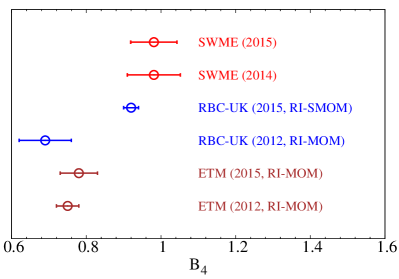
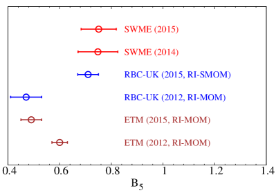
The pattern of results in the Table suggests that the ultimate source of these differences may well be the matching from lattice matrix elements to those in the continuum $\overline{\mathrm{MS}}$ scheme. In our calculation, this error is due to the truncation of matching factors at one-loop order. For $B_{4}$ and $B_{5}$ (the two $B$-parameters which differ from the results obtained using the RI-MOM scheme) our error estimate is taken as the difference between fits using $\tilde{F}_{1}$ and $\tilde{F}_{4}$ fit forms (see Figs. 10 and 11). While we consider this to be a conservative estimate, we cannot rule out that it is an underestimate due to unexpectedly large $\alpha^{2}$ terms in the matching factors. In the case of the calculations using the NPR method, the significant differences between results obtained using RI-MOM and RI-SMOM schemes indicate an underestimate of the associated systematic errors. This could be a problem specifically related to the RI-MOM scheme, where one must subtract unwanted contributions from pion poles, a source of systematic errors absent in the RI-SMOM schemes Lytle et al. (2013). Or it could be due to large truncation errors in the relation between one or both of these schemes and the $\overline{\mathrm{MS}}$ scheme.

Clearly these issues require further investigation. One possibility is for all the calculations to use the same intermediate scheme such as RI-SMOM and then to directly compare results in that scheme. This reduces the dependence on perturbation theory as one does not need to to match to the $\overline{\mathrm{MS}}$ scheme. One would still need to evolve between different scales in the RI-SMOM scheme, but this could also, ultimately, be done non-perturbatively Arthur and Boyle (2011). To these ends we are pursuing the implementation of NPR using staggered fermions Lytle and Sharpe (2013); Kim et al. (2014b); Jeong et al. (2015).