On the Gap and Time Interval between the First Two Maxima of Long Continuous Time Random Walks

Philippe Mounaix philippe.mounaix@cpht.polytechnique.fr Centre de Physique Théorique, UMR 7644 du CNRS, Ecole Polytechnique, 91128 Palaiseau Cedex, France.    Grégory Schehr gregory.schehr@lptms.u-psud.fr Laboratoire de Physique Théorique et Modèles Statistiques, Université Paris-Sud, Bât 100, 91405 Orsay Cedex, France.    Satya N. Majumdar majumdar@lptms.u-psud.fr Laboratoire de Physique Théorique et Modèles Statistiques, Université Paris-Sud, Bât 100, 91405 Orsay Cedex, France.
Abstract

We consider a one-dimensional continuous time random walk (CTRW) on a fixed time interval T𝑇T where at each time step the walker waits a random time τ𝜏\tau, before performing a jump drawn from a symmetric continuous probability distribution function (PDF) f(η)𝑓𝜂f(\eta), of Lévy index 0<μ20𝜇20<\mu\leq 2. Our study includes the case where the waiting time PDF Ψ(τ)Ψ𝜏\Psi(\tau) has a power law tail, Ψ(τ)τ1γproportional-toΨ𝜏superscript𝜏1𝛾\Psi(\tau)\propto\tau^{-1-\gamma}, with 0<γ<10𝛾10<\gamma<1, such that the average time between two consecutive jumps is infinite. The random motion is sub-diffusive if γ<μ/2𝛾𝜇2\gamma<\mu/2 (and super-diffusive if γ>μ/2𝛾𝜇2\gamma>\mu/2). We investigate the joint PDF of the gap g𝑔g between the first two highest positions of the CTRW and the time t𝑡t separating these two maxima. We show that this PDF reaches a stationary limiting joint distribution p(g,t)𝑝𝑔𝑡p(g,t) in the limit of long CTRW, T𝑇T\to\infty. Our exact analytical results show a very rich behavior of this joint PDF in the (γ,μ)𝛾𝜇(\gamma,\mu) plane, which we study in great detail. Our main results are verified by numerical simulations. This work provides a non trivial extension to CTRWs of the recent study in the discrete time setting by Majumdar et al. (J. Stat. Mech. P09013, 2014).

pacs:
05.40.Fb, 02.50.Cw

I Introduction and summary of main results

Recently, there has been a resurgence of interest in extreme value questions for random walks and its variants, particularly in the physics literature AS2005 ; DB09 ; DB11 ; MMS2013 ; MMS2014 ; SLD2010 . This is motivated to a large extent by the observation that extreme value statistics (EVS) plays a crucial role in the physics of complex and disordered systems BM97 ; DM01 . Although the EVS of independent and identically distributed (i.i.d.) random variables is very well understood, much less is known for strongly correlated variables, which is the case frequently encountered in physics. From that point of view, random walks offer a very useful framework where the effects of correlations on EVS can be characterized analytically.

The statistics of the maximal displacement of a random walk (RW) after a given number of steps n𝑛n is now quite well understood, thanks for instance to the Pollaczeck-Spitzer formula Poll ; Spitz , from which precise asymptotic estimates in the large n𝑛n limit can be obtained AS2005 . The full order statistics, i.e. the statistics of the kthsuperscript𝑘thk^{\rm th} maximum for any integer k𝑘k, was investigated in SM2012 in the case of ordinary RWs with a narrow jump distribution (characterized by a Lévy exponent μ=2𝜇2\mu=2). Of particular interest is the gap between two consecutive maxima, which makes it possible to characterize the “crowding” of the walker positions near their maximum. Along this line we recently obtained a complete description of the joint distribution of the gap and time interval between the first two maxima of RWs not only for narrow jump distributions (μ=2𝜇2\mu=2), but also for Lévy flights characterized by a Lévy exponent 0<μ<20𝜇20<\mu<2 MMS2013 ; MMS2014 . Since the characteristic displacement of the walker after n𝑛n time steps grows like n1/μsuperscript𝑛1𝜇n^{1/\mu}, the results of MMS2013 ; MMS2014 are of interest for diffusive (μ=2𝜇2\mu=2) and super-diffusive (0<μ<20𝜇20<\mu<2) processes only, leaving out the important case of sub-diffusive processes. Extending the analysis of MMS2013 ; MMS2014 to sub-diffusive RWs has been one of the motivations for this work.

A common model to describe sub-diffusive processes is the so called continuous time random walk (CTRW). In this model, the walker performs a usual random walk where two consecutive jumps are separated by a certain trapping time τ𝜏\tau. The trapping times are i.i.d. random variables drawn from a common distribution Ψ(τ)Ψ𝜏\Psi(\tau) which has a power law tail Ψ(τ)τ1γproportional-toΨ𝜏superscript𝜏1𝛾\Psi(\tau)\propto\tau^{-1-\gamma} with 0<γ<10𝛾10<\gamma<1. This model, initially suggested by Scher and Montroll in the setting of non-Gaussian transport in disordered electronic systems SM1975 , has been widely used to describe anomalous sub-diffusive dynamics in various complex systems phenomenologically BG90 ; MK2000 . Indeed, for 0<γ<10𝛾10<\gamma<1 the average trapping time between two successive jumps is infinite and, consequently, CTRWs are characterized by an anomalous growth of displacement tγ/μproportional-toabsentsuperscript𝑡𝛾𝜇\propto t^{\gamma/\mu} which is indeed sub-diffusive if γ<μ/2𝛾𝜇2\gamma<\mu/2 (and super-diffusive for γ>μ/2𝛾𝜇2\gamma>\mu/2). The case of a finite average trapping time between two successive jumps corresponds to standard, non sub-diffusive, RWs. The fluctuations of the maximal displacement of CTRWs for μ=2𝜇2\mu=2 and arbitrary γ<1𝛾1\gamma<1 was studied in Ref. SLD2010 using real space renormalization techniques (see also CTB2010 for a Feynman-Kac approach). A precise estimate of the expected value of the maximum of the CTRW was obtained in Ref. FM2012 by combining the results of Ref. AS2005 with the so called ’subordination property’. However, nothing is known about the order statistics, beyond the first maximum, for such CTRWs. In this paper, we provide a complete analytic description of the distribution of the gap and the time interval between the first two maxima of such CTRWs for any values of the parameters 0<μ20𝜇20<\mu\leq 2 and 0<γ<10𝛾10<\gamma<1, as well as for a finite average trapping time between two successive jumps.

We consider a CTRW starting at the origin, x(t=0)=x0=0𝑥𝑡0subscript𝑥00x(t=0)=x_{0}=0, and evolving according to

xi=xi1+ηi,subscript𝑥𝑖subscript𝑥𝑖1subscript𝜂𝑖x_{i}=x_{i-1}+\eta_{i}, (1)

where xisubscript𝑥𝑖x_{i} denotes the walker position between the i𝑖i-th and the (i+1)𝑖1(i+1)-th jumps. The jumps ηisubscript𝜂𝑖\eta_{i} are i.i.d. random variables distributed following a symmetric, bounded and piecewise continuous distribution f(η)𝑓𝜂f(\eta) the Fourier transform of which, f^(k)=+f(η)eikη𝑑η^𝑓𝑘superscriptsubscript𝑓𝜂superscripte𝑖𝑘𝜂differential-d𝜂\hat{f}(k)=\int_{-\infty}^{+\infty}f(\eta){\rm e}^{ik\eta}d\eta, has the small k𝑘k behavior

f^(k)=1|ak|μ+o(|k|μ),^𝑓𝑘1superscript𝑎𝑘𝜇𝑜superscript𝑘𝜇\hat{f}(k)=1-|ak|^{\mu}+o(|k|^{\mu}), (2)

where 0<μ20𝜇20<\mu\leq 2 is the Lévy index and a>0𝑎0a>0 is the characteristic length scale of the jumps. For μ=2𝜇2\mu=2, the variance of the jump distribution σ2=+η2f(η)𝑑ηsuperscript𝜎2superscriptsubscriptsuperscript𝜂2𝑓𝜂differential-d𝜂\sigma^{2}=\int_{-\infty}^{+\infty}\eta^{2}f(\eta)d\eta is well defined and a=σ/2𝑎𝜎2a=\sigma/\sqrt{2}. On the other hand, for 0<μ<20𝜇20<\mu<2, f(η)𝑓𝜂f(\eta) does not possess a well defined second moment because of its heavy tails, f(η)|η|1μproportional-to𝑓𝜂superscript𝜂1𝜇f(\eta)\propto|\eta|^{-1-\mu} (η𝜂\eta\to\infty), and the RW (1) is a Lévy flight of index μ𝜇\mu. The time intervals τisubscript𝜏𝑖\tau_{i} between the (i1)𝑖1(i-1)-th and the i𝑖i-th jumps (τi>0subscript𝜏𝑖0\tau_{i}>0) are i.i.d. random variables, independent of ηisubscript𝜂𝑖\eta_{i}, with PDF Ψ(τ)Ψ𝜏\Psi(\tau) the Laplace transform of which, Ψ^(q)=0+Ψ(τ)exp(qτ)𝑑τ^Ψ𝑞superscriptsubscript0Ψ𝜏𝑞𝜏differential-d𝜏\hat{\Psi}(q)=\int_{0}^{+\infty}\Psi(\tau)\,\exp(-q\tau)\,d\tau, has the small q𝑞q behavior

Ψ^(q)=1(τcq)γ+o(|q|γ),^Ψ𝑞1superscriptsubscript𝜏𝑐𝑞𝛾𝑜superscript𝑞𝛾\hat{\Psi}(q)=1-(\tau_{c}q)^{\gamma}+o(|q|^{\gamma}), (3)

where 0<γ10𝛾10<\gamma\leq 1 and τc>0subscript𝜏𝑐0\tau_{c}>0 is the characteristic time scale of the jumps. For γ=1𝛾1\gamma=1, the mean time between two successive jumps, τ0+τΨ(τ)𝑑τ<+delimited-⟨⟩𝜏superscriptsubscript0𝜏Ψ𝜏differential-d𝜏\langle\tau\rangle\equiv\int_{0}^{+\infty}\tau\Psi(\tau)\,d\tau<+\infty, exists and τc=τsubscript𝜏𝑐delimited-⟨⟩𝜏\tau_{c}=\langle\tau\rangle. For 0<γ<10𝛾10<\gamma<1, the mean time between two successive jumps does not exist. As a function of time, the walker position is thus given by

dx(t)dt=i=1nηiδ(tj=1iτj),𝑑𝑥𝑡𝑑𝑡superscriptsubscript𝑖1𝑛subscript𝜂𝑖𝛿𝑡superscriptsubscript𝑗1𝑖subscript𝜏𝑗\frac{dx(t)}{dt}=\sum_{i=1}^{n}\eta_{i}\,\delta\left(t-\sum_{j=1}^{i}\tau_{j}\right), (4)

with x(0)=0𝑥00x(0)=0 and n𝑛n the total number of jumps in the walk. The solution to (4) is readily found to be given by x(j=1iτj<t<j=1i+1τj)=xi𝑥superscriptsubscript𝑗1𝑖subscript𝜏𝑗𝑡superscriptsubscript𝑗1𝑖1subscript𝜏𝑗subscript𝑥𝑖x(\sum_{j=1}^{i}\tau_{j}<t<\sum_{j=1}^{i+1}\tau_{j})=x_{i} with xisubscript𝑥𝑖x_{i} given by (1).

The goal of the present paper is to provide an exhaustive discussion of the different behaviors of the joint PDF of the gap g𝑔g and time interval t𝑡t between the first two maxima of the walk that may arise in the large n𝑛n limit, depending on the large argument behavior of f(η)𝑓𝜂f(\eta) and Ψ(τ)Ψ𝜏\Psi(\tau). Before entering the details of the calculations, it is useful to summarize our main results. We first show that the joint PDF pn(g,t)subscript𝑝𝑛𝑔𝑡p_{n}(g,t) has a well defined limiting PDF as n𝑛n\to\infty:

limnpn(g,t)=p(g,t),subscript𝑛subscript𝑝𝑛𝑔𝑡𝑝𝑔𝑡\lim_{n\to\infty}p_{n}(g,t)=p(g,t), (5)

where the Laplace transform of p(g,l)𝑝𝑔𝑙p(g,l) with respect to (w.r.t.) t𝑡t is given in Eqs. (20) and (17). Then, we perform a detailed analysis of p(g,t)𝑝𝑔𝑡p(g,t) in the plane (g,t)𝑔𝑡(g,t) for μ𝜇\mu and γ𝛾\gamma in the whole ranges 0<μ20𝜇20<\mu\leq 2 and 0<γ10𝛾10<\gamma\leq 1, and for the three different main classes identified in MMS2014 : (i) slow, (ii) exponentially, and (iii) fast decreasing f(η)𝑓𝜂f(\eta) at large η𝜂\eta.

One of the most remarkable result of this study may be the existence of a scaling form for the joint PDF p(g,t)𝑝𝑔𝑡p(g,t) in the case of a fast decreasing jump distribution (μ=2𝜇2\mu=2), such that f(η+x)f(η)exp(cηδx)similar-to𝑓𝜂𝑥𝑓𝜂𝑐superscript𝜂𝛿𝑥f(\eta+x)\sim f(\eta)\exp(-c\,\eta^{\delta}\,x) for η𝜂\eta\to\infty [see Eq. (68) below for a more precise definition], with 0<γ<10𝛾10<\gamma<1. This class includes the case of a Gaussian jump distribution for which δ=1𝛿1\delta=1. This is a new result, characteristic of CTRWs, without any counterpart in the discrete time RW setting considered in MMS2014 . More specifically, we show that there is a scaling regime g,t1much-greater-than𝑔𝑡1g,\ t\gg 1 with fixed tγ/2gμsuperscript𝑡𝛾2superscript𝑔𝜇t^{\gamma/2}g^{-\mu}, in which p(g,t)𝑝𝑔𝑡p(g,t) takes the scaling form

p(g,t)af(g)2τc(acgδ)3+2/γK((t/τc)γ/2acgδ)(g+andt+),similar-to𝑝𝑔𝑡𝑎𝑓superscript𝑔2subscript𝜏𝑐superscript𝑎𝑐superscript𝑔𝛿32𝛾𝐾superscript𝑡subscript𝜏𝑐𝛾2𝑎𝑐superscript𝑔𝛿𝑔and𝑡p(g,t)\sim\frac{af(g)^{2}}{\tau_{c}(acg^{\delta})^{3+2/\gamma}}K\left(\frac{(t/\tau_{c})^{\gamma/2}}{acg^{\delta}}\right)\ \ \ \ (g\rightarrow+\infty\ {\rm and}\ t\rightarrow+\infty), (6)

with the asymptotic behaviors

K(y){𝒟Iy2(1+1/γ),(y0)𝒟IIy12/γ,(y+)similar-to𝐾𝑦casessubscript𝒟Isuperscript𝑦211𝛾𝑦0subscript𝒟IIsuperscript𝑦12𝛾𝑦K(y)\sim\left\{\begin{array}[]{ll}\mathcal{D}_{\rm I}\,y^{-2(1+1/\gamma)},&(y\rightarrow 0)\\ \mathcal{D}_{\rm II}\,y^{-1-2/\gamma},&(y\rightarrow+\infty)\end{array}\right. (7)

where the amplitudes 𝒟Isubscript𝒟I\mathcal{D}_{\rm I} and 𝒟IIsubscript𝒟II\mathcal{D}_{\rm II} are given in Eqs. (80) and (81), respectively. Physically, the switch from the first to the second behavior (7) around (t/τc)γ/2acgδsimilar-tosuperscript𝑡subscript𝜏𝑐𝛾2𝑎𝑐superscript𝑔𝛿(t/\tau_{c})^{\gamma/2}\sim acg^{\delta} corresponds to the cross-over from a ‘concentration’ – or ‘one-step’ – regime (for (t/τc)γ/2<acgδsuperscript𝑡subscript𝜏𝑐𝛾2𝑎𝑐superscript𝑔𝛿(t/\tau_{c})^{\gamma/2}<acg^{\delta}) where the walker get stuck for a long time t𝑡t at the second maximum and then jumps directly to the first maximum, to a ‘many-steps’ regime (for (t/τc)γ/2>acgδsuperscript𝑡subscript𝜏𝑐𝛾2𝑎𝑐superscript𝑔𝛿(t/\tau_{c})^{\gamma/2}>acg^{\delta}) where she/he travels a long walk of total duration t𝑡t (with many steps) between the second and the first maxima. For γ=1𝛾1\gamma=1, there is no scaling form and (6) is replaced with the uniform expression (84).

An other important result is how the scaling form derived in MMS2014 for a discrete time Lévy flight (see Sec. 4.1 and Appendix D in MMS2014 ) is affected when one switches to a CTRW. Lévy flights have type (i) jump distributions since, for 0<μ<20𝜇20<\mu<2, f(η)𝑓𝜂f(\eta) necessarily has an algebraic, slow decreasing, tail. In this case we show that in the scaling regime g,t1much-greater-than𝑔𝑡1g,\ t\gg 1 with fixed tγgμsuperscript𝑡𝛾superscript𝑔𝜇t^{\gamma}g^{-\mu}, the joint PDF p(g,t)𝑝𝑔𝑡p(g,t) takes the scaling form

p(g,t)1aτc(ag)1+μ(1+1/γ)Fμ,γ(aμtγgμτcγ)(g+andt+),similar-to𝑝𝑔𝑡1𝑎subscript𝜏𝑐superscript𝑎𝑔1𝜇11𝛾subscript𝐹𝜇𝛾superscript𝑎𝜇superscript𝑡𝛾superscript𝑔𝜇superscriptsubscript𝜏𝑐𝛾𝑔and𝑡p(g,t)\sim\frac{1}{a\tau_{c}}\,\left(\frac{a}{g}\right)^{1+\mu(1+1/\gamma)}F_{\mu,\,\gamma}\left(\frac{a^{\mu}t^{\gamma}}{g^{\mu}\tau_{c}^{\gamma}}\right)\ \ \ \ (g\rightarrow+\infty\ {\rm and}\ t\rightarrow+\infty), (8)

with the asymptotic behaviors

Fμ,γ(y){𝒞Iy1/μ1/γ,1Int(γ)<μ<2,𝒞IIy11/γlny,μ=1,𝒞IIIy11/γ,0<μ<1,(y+),similar-tosubscript𝐹𝜇𝛾𝑦casessubscript𝒞Isuperscript𝑦1𝜇1𝛾1Int𝛾𝜇2subscript𝒞IIsuperscript𝑦11𝛾𝑦𝜇1subscript𝒞IIIsuperscript𝑦11𝛾0𝜇1𝑦F_{\mu,\,\gamma}(y)\sim\left\{\begin{array}[]{ll}\mathcal{C}_{\rm I}\,y^{-1/\mu-1/\gamma},&1-{\rm Int}(\gamma)<\mu<2,\\ \mathcal{C}_{\rm II}\,y^{-1-1/\gamma}\ln y,&\mu=1,\\ \mathcal{C}_{\rm III}\,y^{-1-1/\gamma},&0<\mu<1,\end{array}\right.\ \ \ \ (y\rightarrow+\infty), (9)

and

Fμ,γ(y)𝒞IVy1/21/γ,(y0),similar-tosubscript𝐹𝜇𝛾𝑦subscript𝒞IVsuperscript𝑦121𝛾𝑦0F_{\mu,\,\gamma}(y)\sim\mathcal{C}_{\rm IV}\,y^{1/2-1/\gamma},\ \ \ \ (y\rightarrow 0), (10)

where Int(γ)Int𝛾{\rm Int}(\gamma) in the first line of (9) denotes the integer part of γ𝛾\gamma and the last two lines are for 0<γ<10𝛾10<\gamma<1 only. It can be checked that for γ=1𝛾1\gamma=1, Eqs. (8), (9), and (10) reduce to Eqs. (87), (88), and (90) of MMS2014 in which the number of jumps between the first two maxima, l𝑙l, is merely replaced with t/τc𝑡subscript𝜏𝑐t/\tau_{c}, as expected from simple law of large number arguments giving lt/τc𝑙𝑡subscript𝜏𝑐l\rightarrow t/\tau_{c} as t+𝑡t\rightarrow+\infty. Our results provide thus a non trivial extension of the ones in MMS2014 to the case 0<γ<10𝛾10<\gamma<1 in which the mean time between two successive jumps does not exist and law of large number arguments cannot be used.

Finally, by integration of the joint PDF p(g,t)𝑝𝑔𝑡p(g,t) over g𝑔g, one finds that the marginal distribution ptime(t)subscript𝑝time𝑡p_{\rm time}(t) displays a power law tail with logarithmic corrections and an exponent depending only on μ𝜇\mu and γ𝛾\gamma. Namely, for γ=1𝛾1\gamma=1 one finds

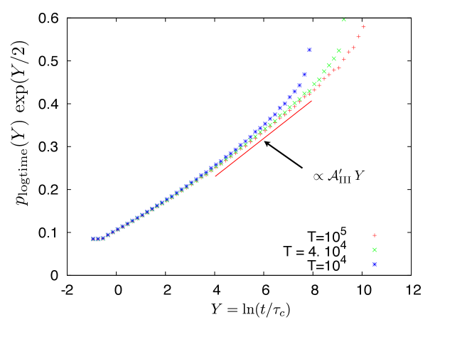
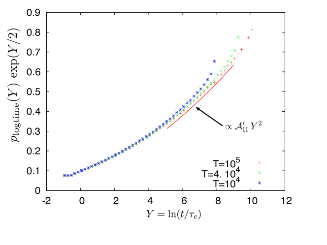
ptime(t)1τc×{𝒜I(t/τc)11/μ,1<μ2,𝒜IIln(t/τc)(t/τc)2,μ=1,𝒜III(t/τc)2,0<μ<1,(t+),similar-tosubscript𝑝time𝑡1subscript𝜏𝑐casessubscript𝒜Isuperscript𝑡subscript𝜏𝑐11𝜇1𝜇2subscript𝒜II𝑡subscript𝜏𝑐superscript𝑡subscript𝜏𝑐2𝜇1subscript𝒜IIIsuperscript𝑡subscript𝜏𝑐20𝜇1𝑡p_{\rm time}(t)\sim\frac{1}{\tau_{c}}\times\left\{\begin{array}[]{ll}\mathcal{A}_{\rm I}\,(t/\tau_{c})^{-1-1/\mu},&1<\mu\leq 2,\\ \mathcal{A}_{\rm II}\,\ln(t/\tau_{c})\,(t/\tau_{c})^{-2},&\mu=1,\\ \mathcal{A}_{\rm III}\,(t/\tau_{c})^{-2},&0<\mu<1,\end{array}\right.\ \ \ \ (t\rightarrow+\infty), (11)

where the amplitudes 𝒜Isubscript𝒜I{\cal A}_{\rm I}, 𝒜IIsubscript𝒜II{\cal A}_{\rm II} and 𝒜IIIsubscript𝒜III{\cal A}_{\rm III} are given in Eq. (91), and for 0<γ<10𝛾10<\gamma<1 one has

ptime(t)1τc×{𝒜I(t/τc)1γ/μ,1<μ2,𝒜IIln2(t/τc)(t/τc)1γ,μ=1,𝒜IIIln(t/τc)(t/τc)1γ,0<μ<1,(t+),similar-tosubscript𝑝time𝑡1subscript𝜏𝑐casessuperscriptsubscript𝒜Isuperscript𝑡subscript𝜏𝑐1𝛾𝜇1𝜇2superscriptsubscript𝒜IIsuperscript2𝑡subscript𝜏𝑐superscript𝑡subscript𝜏𝑐1𝛾𝜇1superscriptsubscript𝒜III𝑡subscript𝜏𝑐superscript𝑡subscript𝜏𝑐1𝛾0𝜇1𝑡p_{\rm time}(t)\sim\frac{1}{\tau_{c}}\times\left\{\begin{array}[]{ll}\mathcal{A}_{\rm I}^{\prime}\,(t/\tau_{c})^{-1-\gamma/\mu},&1<\mu\leq 2,\\ \mathcal{A}_{\rm II}^{\prime}\,\ln^{2}(t/\tau_{c})\,(t/\tau_{c})^{-1-\gamma},&\mu=1,\\ \mathcal{A}_{\rm III}^{\prime}\,\ln(t/\tau_{c})\,(t/\tau_{c})^{-1-\gamma},&0<\mu<1,\end{array}\right.\ \ \ \ (t\rightarrow+\infty), (12)

where the amplitudes 𝒜Isuperscriptsubscript𝒜I{\cal A}_{\rm I}^{\prime}, 𝒜IIsuperscriptsubscript𝒜II{\cal A}_{\rm II}^{\prime} and 𝒜IIIsuperscriptsubscript𝒜III{\cal A}_{\rm III}^{\prime} are given in Eq. (97). Again, it can be checked that Eq. (11) is nothing but Eq. (112) in MMS2014 with l=t/τc𝑙𝑡subscript𝜏𝑐l=t/\tau_{c}, as expected (cf. the end of the preceding paragraph). Note that for μ=2𝜇2\mu=2 and γ=1𝛾1\gamma=1, one has ptime(t)t3/2proportional-tosubscript𝑝time𝑡superscript𝑡32p_{\rm time}(t)\propto t^{-3/2} whatever the distributions f(η)𝑓𝜂f(\eta) and Ψ(τ)Ψ𝜏\Psi(\tau) possessing a second and a first moment, respectively. The third lines of (11) and (12) reveal an interesting freezing phenomenon, as a function of μ𝜇\mu, of the large t𝑡t behavior of ptime(t)subscript𝑝time𝑡p_{\rm time}(t) as μ𝜇\mu decreases past the value μc=1subscript𝜇𝑐1\mu_{c}=1. It follows in particular from (11) and (12) that the first moment of ptime(t)subscript𝑝time𝑡p_{\rm time}(t) is never defined. This means that, although the typical size of t𝑡t is 𝒪(1)𝒪1{\cal O}(1), its average diverges with the total duration, T𝑇T, of the random walk. For 0<γ10𝛾10<\gamma\leq 1 one can estimate from (11) and (12) that |t|T1γ/μsimilar-todelimited-⟨⟩𝑡superscript𝑇1𝛾𝜇\langle|t|\rangle\sim T^{1-\gamma/\mu} for 1<μ21𝜇21<\mu\leq 2, while |t|T1γlogTsimilar-todelimited-⟨⟩𝑡superscript𝑇1𝛾𝑇\langle|t|\rangle\sim T^{1-\gamma}\log{T} for 0<μ<10𝜇10<\mu<1 and |t|T1γ(lnT)2similar-todelimited-⟨⟩𝑡superscript𝑇1𝛾superscript𝑇2\langle|t|\rangle\sim T^{1-\gamma}(\ln{T})^{2} for μ=1𝜇1\mu=1. Table 1 summarizes the functional dependence of the different asymptotic behaviors of ptime(t)subscript𝑝time𝑡p_{\rm time}(t) at large t𝑡t in the (μ,γ)𝜇𝛾(\mu,\gamma) plane.

ptime(t)proportional-tosubscript𝑝time𝑡absentp_{\rm time}(t)\propto 1<μ21𝜇21<\mu\leq 2 μ=1𝜇1\mu=1 0<μ<10𝜇10<\mu<1
γ=1𝛾1\gamma=1 t11/μsuperscript𝑡11𝜇t^{-1-1/\mu} t2lntsuperscript𝑡2𝑡t^{-2}\ln t t2superscript𝑡2t^{-2}
0<γ<10𝛾10<\gamma<1 t1γ/μsuperscript𝑡1𝛾𝜇t^{-1-\gamma/\mu} t1γ(lnt)2superscript𝑡1𝛾superscript𝑡2t^{-1-\gamma}(\ln t)^{2} t1γlntsuperscript𝑡1𝛾𝑡t^{-1-\gamma}\ln t
Table 1: Functional dependence of the different asymptotic behaviors of ptime(t)subscript𝑝time𝑡p_{\rm time}(t) at large t𝑡t in the (μ,γ)𝜇𝛾(\mu,\gamma) plane.

Note that the marginal distribution of the gap between the first two maxima, pgap(g)subscript𝑝gap𝑔p_{\rm gap}(g), obtained by integration of the joint PDF p(g,t)𝑝𝑔𝑡p(g,t) over t𝑡t, does not depend on Ψ(τ)Ψ𝜏\Psi(\tau) (hence on γ𝛾\gamma) and is the same as the one already studied in Sec. 3 of Ref. MMS2014 in the discrete time RW setting.

The outline of the paper is as follows. In Section II we give the Laplace transform of p(g,t)𝑝𝑔𝑡p(g,t) with respect to t𝑡t for a free-end random walk and a random bridge in which the walker is conditioned to return to x=0𝑥0x=0 at the end of the walk. Section III deals with the asymptotic behavior of p(g,t)𝑝𝑔𝑡p(g,t) for large t𝑡t at fixed g𝑔g, from which we derive, in Section IV, the asymptotic behavior of p(g,t)𝑝𝑔𝑡p(g,t) for a Lévy flight at large t𝑡t then large g𝑔g. The asymptotic behavior of p(g,t)𝑝𝑔𝑡p(g,t) for large g𝑔g is investigated in Section V for three classes of jump distributions encompassing a wide range of jumps of practical interest. It is shown in Section V.3 that when the jump distribution has a fast decreasing tail, the behavior of p(g,l)𝑝𝑔𝑙p(g,l) when both g𝑔g and l𝑙l are large takes on a scaling form capturing the existence of two complementary regimes, one dominated by walks with only one step between the first two maxima, and the other dominated by walks with many steps between the first two maxima. In Section VI we give the scaling form of the asymptotic behavior of p(g,t)𝑝𝑔𝑡p(g,t) for a Lévy flight at large t𝑡t and g𝑔g. In Section VII we use the results obtained in Sections III and VI to determine the large t𝑡t behavior of ptime(t)subscript𝑝time𝑡p_{\rm time}(t) and show its freezing when the random walk is a Lévy flight with index 0<μ<10𝜇10<\mu<1. Finally, Section VIII is devoted to the comparison of our analytical results with numerical simulations.

II Laplace transform of 𝒑(𝒈,𝒕)𝒑𝒈𝒕\bm{p(g,t)} with respect to 𝒕𝒕\bm{t} for a free-end random walk and a random bridge

Let pn(g,t)subscript𝑝𝑛𝑔𝑡p_{n}(g,t) denote the joint PDF of the gap, g𝑔g, and the time interval, t𝑡t, between the first two maxima of a continuous time random walk after n𝑛n steps. Since pn(g,t)=pn(g,t)subscript𝑝𝑛𝑔𝑡subscript𝑝𝑛𝑔𝑡p_{n}(g,-t)=p_{n}(g,t) we will restrict ourselves to t>0𝑡0t>0 without loss of generality. Let l𝑙l denote the number of jumps between the first to maxima. For t>0𝑡0t>0 one has

pn(g,t)=0<lnpn(g,l,t)=0<lnp(t|g,l)pn(g,l)=0<lnp(t|l)pn(g,l),subscript𝑝𝑛𝑔𝑡subscript0𝑙𝑛subscript𝑝𝑛𝑔𝑙𝑡subscript0𝑙𝑛𝑝conditional𝑡𝑔𝑙subscript𝑝𝑛𝑔𝑙subscript0𝑙𝑛𝑝conditional𝑡𝑙subscript𝑝𝑛𝑔𝑙p_{n}(g,t)=\sum_{0<l\leq n}p_{n}(g,l,t)=\sum_{0<l\leq n}p(t|g,l)\,p_{n}(g,l)=\sum_{0<l\leq n}p(t|l)\,p_{n}(g,l), (13)

where p(t|l)𝑝conditional𝑡𝑙p(t|l) has the Laplace transform

p^(q|l)^𝑝conditional𝑞𝑙\displaystyle\hat{p}(q|l) =\displaystyle= 0+p(t|l)exp(qt)𝑑t=0+δ(ti=1lτi)exp(qt)𝑑tsuperscriptsubscript0𝑝conditional𝑡𝑙𝑞𝑡differential-d𝑡superscriptsubscript0delimited-⟨⟩𝛿𝑡superscriptsubscript𝑖1𝑙subscript𝜏𝑖𝑞𝑡differential-d𝑡\displaystyle\int_{0}^{+\infty}p(t|l)\,\exp(-qt)\,dt=\int_{0}^{+\infty}\left\langle\delta(t-\sum_{i=1}^{l}\tau_{i})\right\rangle\,\exp(-qt)\,dt (14)
=\displaystyle= i=1lexp(qτi)=Ψ^(q)l.superscriptsubscriptproduct𝑖1𝑙delimited-⟨⟩𝑞subscript𝜏𝑖^Ψsuperscript𝑞𝑙\displaystyle\prod_{i=1}^{l}\left\langle\exp(-q\tau_{i})\right\rangle=\hat{\Psi}(q)^{l}.

Taking the Laplace transform of (13) with respect to t𝑡t and using (14) one gets

p^n(g,q)=0+pn(g,t)exp(qt)𝑑t=0<lnΨ^(q)lpn(g,l)=p~n(g,Ψ^(q)),subscript^𝑝𝑛𝑔𝑞superscriptsubscript0subscript𝑝𝑛𝑔𝑡𝑞𝑡differential-d𝑡subscript0𝑙𝑛^Ψsuperscript𝑞𝑙subscript𝑝𝑛𝑔𝑙subscript~𝑝𝑛𝑔^Ψ𝑞\hat{p}_{n}(g,q)=\int_{0}^{+\infty}p_{n}(g,t)\,\exp(-qt)\,dt=\sum_{0<l\leq n}\hat{\Psi}(q)^{l}\,p_{n}(g,l)=\tilde{p}_{n}(g,\hat{\Psi}(q)), (15)

where p~n(g,s)=0<lnpn(g,l)slsubscript~𝑝𝑛𝑔𝑠subscript0𝑙𝑛subscript𝑝𝑛𝑔𝑙superscript𝑠𝑙\tilde{p}_{n}(g,s)=\sum_{0<l\leq n}p_{n}(g,l)\,s^{l} is the generating function of pn(g,l)subscript𝑝𝑛𝑔𝑙p_{n}(g,l) with respect to l>0𝑙0l>0. The large n𝑛n limit of (15) can then be readily obtained from the main result of MMS2014 according to which p~(g,s)=limn+p~n(g,s)~𝑝𝑔𝑠subscript𝑛subscript~𝑝𝑛𝑔𝑠\tilde{p}(g,s)=\lim_{n\rightarrow+\infty}\tilde{p}_{n}(g,s) exists and is given by

p~(g,s)=I1(g,s)I2(g),~𝑝𝑔𝑠subscript𝐼1𝑔𝑠subscript𝐼2𝑔\tilde{p}(g,s)=I_{1}(g,s)I_{2}(g), (16)

with

I1(g,s)=s0+u(y,s)f(g+y)𝑑y,I2(g)=0+h(x,1)f(g+x)𝑑x,subscript𝐼1𝑔𝑠𝑠superscriptsubscript0𝑢𝑦𝑠𝑓𝑔𝑦differential-d𝑦subscript𝐼2𝑔superscriptsubscript0𝑥1𝑓𝑔𝑥differential-d𝑥\begin{array}[]{l}I_{1}(g,s)=s\int_{0}^{+\infty}u(y,s)f(g+y)\,dy,\\ I_{2}(g)=\int_{0}^{+\infty}h(x,1)f(g+x)\,dx,\end{array} (17)

where the functions u(x,s)𝑢𝑥𝑠u(x,s) and h(x,s)𝑥𝑠h(x,s) are the inverse Laplace transforms of ϕ(λ,s)italic-ϕ𝜆𝑠\phi(\lambda,s) and ϕ(λ,s)/λitalic-ϕ𝜆𝑠𝜆\phi(\lambda,s)/\lambda, respectively:

0+u(x,s)eλx𝑑x=ϕ(λ,s),0+h(x,s)eλx𝑑x=ϕ(λ,s)/λ,superscriptsubscript0𝑢𝑥𝑠superscripte𝜆𝑥differential-d𝑥italic-ϕ𝜆𝑠superscriptsubscript0𝑥𝑠superscripte𝜆𝑥differential-d𝑥italic-ϕ𝜆𝑠𝜆\begin{array}[]{l}\int_{0}^{+\infty}u(x,s){\rm e}^{-\lambda x}dx=\phi(\lambda,s),\\ \int_{0}^{+\infty}h(x,s){\rm e}^{-\lambda x}dx=\phi(\lambda,s)/\lambda,\end{array} (18)

with

ϕ(λ,s)=exp(λπ0+ln[1sf^(k)]k2+λ2𝑑k).italic-ϕ𝜆𝑠𝜆𝜋superscriptsubscript01𝑠^𝑓𝑘superscript𝑘2superscript𝜆2differential-d𝑘\phi(\lambda,s)=\exp\left(-\frac{\lambda}{\pi}\int_{0}^{+\infty}\frac{\ln[1-s\hat{f}(k)]}{k^{2}+\lambda^{2}}\,dk\right). (19)

Injecting this result into the large n𝑛n limit of (15) yields

p^(g,q)=limn+p^n(g,q)=p~(g,Ψ^(q))=I1(g,Ψ^(q))I2(g).^𝑝𝑔𝑞subscript𝑛subscript^𝑝𝑛𝑔𝑞~𝑝𝑔^Ψ𝑞subscript𝐼1𝑔^Ψ𝑞subscript𝐼2𝑔\hat{p}(g,q)=\lim_{n\rightarrow+\infty}\hat{p}_{n}(g,q)=\tilde{p}(g,\hat{\Psi}(q))=I_{1}(g,\hat{\Psi}(q))I_{2}(g). (20)

Thus, pn(g,t)subscript𝑝𝑛𝑔𝑡p_{n}(g,t) converges to a limiting distribution p(g,t)𝑝𝑔𝑡p(g,t) as n+𝑛n\rightarrow+\infty whose Laplace transform with respect to t𝑡t, p^(g,q)=0+p(g,t)exp(qt)𝑑t^𝑝𝑔𝑞superscriptsubscript0𝑝𝑔𝑡𝑞𝑡differential-d𝑡\hat{p}(g,q)=\int_{0}^{+\infty}p(g,t)\,\exp(-qt)\,dt, is given by (20).

It was proved in MMS2014 that the expression (16) of p~(g,s)~𝑝𝑔𝑠\tilde{p}(g,s) actually holds for both free-end random walks and random bridges in which the walker is conditioned to return to x=0𝑥0x=0 at the end of the walk. Since, for a given Ψ(τ)Ψ𝜏\Psi(\tau), p^(g,q)^𝑝𝑔𝑞\hat{p}(g,q) is entirely determined by p~(g,s)~𝑝𝑔𝑠\tilde{p}(g,s) through (20), it follows immediately that the expression of p^(g,q)^𝑝𝑔𝑞\hat{p}(g,q), hence the one of the limiting joint PDF p(g,t)𝑝𝑔𝑡p(g,t), is exactly the same for free-end walks and bridges. Therefore, all the results obtained in the following apply to free-end random walks as well as to random bridges without any modification.

III Asymptotic behavior of 𝒑(𝒈,𝒕)𝒑𝒈𝒕\bm{p(g,t)} for large 𝒕𝒕\bm{t} at fixed 𝒈𝒈\bm{g}

Sections III to VI are devoted to the asymptotic behavior of the joint PDF p(g,t)𝑝𝑔𝑡p(g,t) when either g𝑔g or t𝑡t (or both) is large. From the results obtained for the large t𝑡t behavior of p(g,t)𝑝𝑔𝑡p(g,t) it will then be possible to derive the large t𝑡t behavior of the marginal distribution ptime(t)=0+p(g,t)𝑑gsubscript𝑝time𝑡superscriptsubscript0𝑝𝑔𝑡differential-d𝑔p_{\rm time}(t)=\int_{0}^{+\infty}p(g,t)\,dg, which will be the subject of Sec. VII.

First, we consider the limit t+𝑡t\rightarrow+\infty at fixed g𝑔g. As we will see, the behavior of p(g,t)𝑝𝑔𝑡p(g,t) in this limit depends on the value of γ𝛾\gamma, leading to new, non trivial, asymptotic expressions if 0<γ<10𝛾10<\gamma<1.

III.1 𝜸=𝟏𝜸1\bm{\gamma=1}

In this case the mean time between two successive jumps, τ=τcdelimited-⟨⟩𝜏subscript𝜏𝑐\langle\tau\rangle=\tau_{c}, exists and by a simple law of large number argument, the large t𝑡t behavior of p(g,t)𝑝𝑔𝑡p(g,t) can be expected to be given by τc1p(g,l=t/τc)superscriptsubscript𝜏𝑐1𝑝𝑔𝑙𝑡subscript𝜏𝑐\tau_{c}^{-1}p(g,l=t/\tau_{c}), where l=t/τc𝑙𝑡subscript𝜏𝑐l=t/\tau_{c} is large. Let us check this result explicitly by comparing the large t𝑡t behavior of p(g,t)𝑝𝑔𝑡p(g,t) and the large l𝑙l behavior of p(g,l)𝑝𝑔𝑙p(g,l).

The behavior of p(g,t)𝑝𝑔𝑡p(g,t) at large t𝑡t is determined by the one of p^(g,q)^𝑝𝑔𝑞\hat{p}(g,q) at small q𝑞q. Thus, from (20) and (3) with γ=1𝛾1\gamma=1, one has

p(g,t)𝑝𝑔𝑡\displaystyle p(g,t) =\displaystyle= 12iπp~(g,Ψ^(q))exp(qt)𝑑q12𝑖𝜋subscript~𝑝𝑔^Ψ𝑞𝑞𝑡differential-d𝑞\displaystyle\frac{1}{2i\pi}\int_{\mathcal{L}}\tilde{p}(g,\hat{\Psi}(q))\,\exp(qt)\,dq (21)
similar-to\displaystyle\sim 12iπp~(g,1τcq)exp(qt)𝑑q(t+)12𝑖𝜋subscript~𝑝𝑔1subscript𝜏𝑐𝑞𝑞𝑡differential-d𝑞𝑡\displaystyle\frac{1}{2i\pi}\int_{\mathcal{L}}\tilde{p}(g,1-\tau_{c}q)\,\exp(qt)\,dq\ \ \ \ (t\rightarrow+\infty)
=\displaystyle= 12iπτcp~(g,1q)exp(qtτc)𝑑q,12𝑖𝜋subscript𝜏𝑐subscript~𝑝𝑔1𝑞𝑞𝑡subscript𝜏𝑐differential-d𝑞\displaystyle\frac{1}{2i\pi\,\tau_{c}}\int_{\mathcal{L}}\tilde{p}(g,1-q)\,\exp\left(\frac{qt}{\tau_{c}}\right)\,dq,

where we have made the change of variable qq/τc𝑞𝑞subscript𝜏𝑐q\rightarrow q/\tau_{c}. Similarly, for large l𝑙l the behavior of p(g,l)𝑝𝑔𝑙p(g,l) is determined by the one of p~(g,s)~𝑝𝑔𝑠\tilde{p}(g,s) near s=1𝑠1s=1. Making the change of variable s=exp(q)𝑠𝑞s=\exp(-q) one gets

p(g,l)𝑝𝑔𝑙\displaystyle p(g,l) =\displaystyle= 12iπp~(g,s)sl+1𝑑s12𝑖𝜋contour-integral~𝑝𝑔𝑠superscript𝑠𝑙1differential-d𝑠\displaystyle\frac{1}{2i\pi}\oint\frac{\tilde{p}(g,s)}{s^{l+1}}ds (22)
=\displaystyle= 12iπiπ+0+iπ+0p~(g,exp(q))exp(ql)𝑑q12𝑖𝜋superscriptsubscript𝑖𝜋0𝑖𝜋0~𝑝𝑔𝑞𝑞𝑙differential-d𝑞\displaystyle\frac{1}{2i\pi}\int_{-i\pi+0}^{+i\pi+0}\tilde{p}(g,\exp(-q))\,\exp(ql)\,dq
similar-to\displaystyle\sim 12iπp~(g,1q)exp(ql)𝑑q(l+).12𝑖𝜋subscript~𝑝𝑔1𝑞𝑞𝑙differential-d𝑞𝑙\displaystyle\frac{1}{2i\pi}\int_{\mathcal{L}}\tilde{p}(g,1-q)\,\exp(ql)\,dq\ \ \ \ (l\rightarrow+\infty).

Comparing Eqs. (21) and (22), one obtains the expected expression

p(g,t)1τcp(g,l=tτc)(t+).similar-to𝑝𝑔𝑡1subscript𝜏𝑐𝑝𝑔𝑙𝑡subscript𝜏𝑐𝑡p(g,t)\sim\frac{1}{\tau_{c}}p\left(g,l=\frac{t}{\tau_{c}}\right)\ \ \ \ (t\rightarrow+\infty). (23)

Finally, Eq. (65) of MMS2014 together with Eq. (23) above yield, for all 0<μ20𝜇20<\mu\leq 2,

p(g,t)Γ(1+1/μ)πaτcI2(g)2(t/τc)1+1/μ(t+).similar-to𝑝𝑔𝑡Γ11𝜇𝜋𝑎subscript𝜏𝑐subscript𝐼2superscript𝑔2superscript𝑡subscript𝜏𝑐11𝜇𝑡p(g,t)\sim\frac{\Gamma(1+1/\mu)}{\pi a\tau_{c}}\,\frac{I_{2}(g)^{2}}{(t/\tau_{c})^{1+1/\mu}}\ \ \ \ (t\rightarrow+\infty). (24)

III.2 𝟎<𝜸<𝟏0𝜸1\bm{0<\gamma<1}

If 0<γ<10𝛾10<\gamma<1 the mean time between two successive jumps, τ=+delimited-⟨⟩𝜏\langle\tau\rangle=+\infty, does not exist and the large t𝑡t behavior of p(g,t)𝑝𝑔𝑡p(g,t) is no longer related to p(g,l)𝑝𝑔𝑙p(g,l) by the simple expression (23). Following the same line as for Eq. (21) with 0<γ<10𝛾10<\gamma<1, one now has

p(g,t)𝑝𝑔𝑡\displaystyle p(g,t) =\displaystyle= 12iπp~(g,Ψ^(q))exp(qt)𝑑q12𝑖𝜋subscript~𝑝𝑔^Ψ𝑞𝑞𝑡differential-d𝑞\displaystyle\frac{1}{2i\pi}\int_{\mathcal{L}}\tilde{p}(g,\hat{\Psi}(q))\,\exp(qt)\,dq (25)
similar-to\displaystyle\sim 12iπp~(g,1(τcq)γ)exp(qt)𝑑q(t+)12𝑖𝜋subscript~𝑝𝑔1superscriptsubscript𝜏𝑐𝑞𝛾𝑞𝑡differential-d𝑞𝑡\displaystyle\frac{1}{2i\pi}\int_{\mathcal{L}}\tilde{p}(g,1-(\tau_{c}q)^{\gamma})\,\exp(qt)\,dq\ \ \ \ (t\rightarrow+\infty)
=\displaystyle= 12iπτcp~(g,1qγ)exp(qtτc)𝑑q,12𝑖𝜋subscript𝜏𝑐subscript~𝑝𝑔1superscript𝑞𝛾𝑞𝑡subscript𝜏𝑐differential-d𝑞\displaystyle\frac{1}{2i\pi\,\tau_{c}}\int_{\mathcal{L}}\tilde{p}(g,1-q^{\gamma})\,\exp\left(\frac{qt}{\tau_{c}}\right)\,dq,

where we have made the change of variable qq/τc𝑞𝑞subscript𝜏𝑐q\rightarrow q/\tau_{c}. It remains to compute the inverse Laplace transform on the right-hand side of (25). One finds three different regimes depending on the value of μ𝜇\mu.

III.2.1 𝟏<𝝁𝟐1𝝁2\bm{1<\mu\leq 2}

For 1<μ21𝜇21<\mu\leq 2 the behavior of p~(g,s)~𝑝𝑔𝑠\tilde{p}(g,s) near s=1𝑠1s=1 is given by, (see Eq. (63) in MMS2014 ),

p~(g,s)p~(g,1)aμI2(g)2(1s)1/μ(s1),similar-to~𝑝𝑔𝑠~𝑝𝑔1subscript𝑎𝜇subscript𝐼2superscript𝑔2superscript1𝑠1𝜇𝑠1\tilde{p}(g,s)-\tilde{p}(g,1)\sim-a_{\mu}I_{2}(g)^{2}(1-s)^{1/\mu}\ \ \ \ (s\rightarrow 1), (26)

with aμ=1/[asin(π/μ)]subscript𝑎𝜇1delimited-[]𝑎𝜋𝜇a_{\mu}=1/[a\sin(\pi/\mu)]. Injecting (26) into (25) yields

p(g,t)aμI2(g)22iπτcqγ/μexp(qtτc)𝑑q(t+).similar-to𝑝𝑔𝑡subscript𝑎𝜇subscript𝐼2superscript𝑔22𝑖𝜋subscript𝜏𝑐subscriptsuperscript𝑞𝛾𝜇𝑞𝑡subscript𝜏𝑐differential-d𝑞𝑡p(g,t)\sim-\frac{a_{\mu}I_{2}(g)^{2}}{2i\pi\,\tau_{c}}\int_{\mathcal{L}}q^{\gamma/\mu}\,\exp\left(\frac{qt}{\tau_{c}}\right)\,dq\ \ \ \ (t\rightarrow+\infty). (27)

Performing then the inverse Laplace transform in (27) and using the reflection formula Γ(z)Γ(z+1)=π/sin(πz)Γ𝑧Γ𝑧1𝜋𝜋𝑧\Gamma(-z)\Gamma(z+1)=-\pi/\sin(\pi z) one obtains, for all 1<μ21𝜇21<\mu\leq 2,

p(g,t)sin(πγ/μ)sin(π/μ)Γ(1+γ/μ)πaτcI2(g)2(t/τc)1+γ/μ(t+).similar-to𝑝𝑔𝑡𝜋𝛾𝜇𝜋𝜇Γ1𝛾𝜇𝜋𝑎subscript𝜏𝑐subscript𝐼2superscript𝑔2superscript𝑡subscript𝜏𝑐1𝛾𝜇𝑡p(g,t)\sim\frac{\sin(\pi\gamma/\mu)}{\sin(\pi/\mu)}\,\frac{\Gamma(1+\gamma/\mu)}{\pi a\tau_{c}}\,\frac{I_{2}(g)^{2}}{(t/\tau_{c})^{1+\gamma/\mu}}\ \ \ \ (t\rightarrow+\infty). (28)

Note that the exponent of t𝑡t in (28) depends on μ𝜇\mu and (28) tends to (24) as γ1𝛾1\gamma\rightarrow 1.

III.2.2 𝟎<𝝁<𝟏0𝝁1\bm{0<\mu<1}

For 0<μ<10𝜇10<\mu<1 the behavior of p~(g,s)~𝑝𝑔𝑠\tilde{p}(g,s) near s=1𝑠1s=1 reads, (see Eqs. (63) and (C9) in MMS2014 ),

p~(g,s)p~(g,1)I2(g)J1(g)(1s)(s1),similar-to~𝑝𝑔𝑠~𝑝𝑔1subscript𝐼2𝑔subscript𝐽1𝑔1𝑠𝑠1\tilde{p}(g,s)-\tilde{p}(g,1)\sim-I_{2}(g)J_{1}(g)(1-s)\ \ \ \ (s\rightarrow 1), (29)

with

J1(g)=0+w1(x)f(g+x)𝑑x,subscript𝐽1𝑔superscriptsubscript0subscript𝑤1𝑥𝑓𝑔𝑥differential-d𝑥J_{1}(g)=\int_{0}^{+\infty}w_{1}(x)\,f(g+x)\,dx, (30)

where w1(x)subscript𝑤1𝑥w_{1}(x) is defined by its Laplace transform

0+w1(x)eλx𝑑x=λϕ(λ,1)π0+F^(k)k2+λ2𝑑k,superscriptsubscript0subscript𝑤1𝑥superscripte𝜆𝑥differential-d𝑥𝜆italic-ϕ𝜆1𝜋superscriptsubscript0^𝐹𝑘superscript𝑘2superscript𝜆2differential-d𝑘\int_{0}^{+\infty}w_{1}(x){\rm e}^{-\lambda x}dx=\frac{\lambda\phi(\lambda,1)}{\pi}\int_{0}^{+\infty}\frac{\hat{F}(k)}{k^{2}+\lambda^{2}}\,dk, (31)

with F^(k)=f^(k)/(1f^(k))^𝐹𝑘^𝑓𝑘1^𝑓𝑘\hat{F}(k)=\hat{f}(k)/(1-\hat{f}(k)). Equations (25) and (29) now yield

p(g,t)I2(g)J1(g)2iπτcqγexp(qtτc)𝑑q(t+),similar-to𝑝𝑔𝑡subscript𝐼2𝑔subscript𝐽1𝑔2𝑖𝜋subscript𝜏𝑐subscriptsuperscript𝑞𝛾𝑞𝑡subscript𝜏𝑐differential-d𝑞𝑡p(g,t)\sim-\frac{I_{2}(g)J_{1}(g)}{2i\pi\,\tau_{c}}\int_{\mathcal{L}}q^{\gamma}\,\exp\left(\frac{qt}{\tau_{c}}\right)\,dq\ \ \ \ (t\rightarrow+\infty), (32)

which replaces Eq. (28). Performing the inverse Laplace transform in (32) and using the reflection formula Γ(z)Γ(z+1)=π/sin(πz)Γ𝑧Γ𝑧1𝜋𝜋𝑧\Gamma(-z)\Gamma(z+1)=-\pi/\sin(\pi z) one obtains, for all 0<μ<10𝜇10<\mu<1,

p(g,t)sin(πγ)Γ(1+γ)πτcI2(g)J1(g)(t/τc)1+γ(t+).similar-to𝑝𝑔𝑡𝜋𝛾Γ1𝛾𝜋subscript𝜏𝑐subscript𝐼2𝑔subscript𝐽1𝑔superscript𝑡subscript𝜏𝑐1𝛾𝑡p(g,t)\sim\frac{\sin(\pi\gamma)\,\Gamma(1+\gamma)}{\pi\tau_{c}}\,\frac{I_{2}(g)J_{1}(g)}{(t/\tau_{c})^{1+\gamma}}\ \ \ \ (t\rightarrow+\infty). (33)

Note that the exponent of t𝑡t in (33) does not depend on μ𝜇\mu, unlike its counterpart in Eq. (28). It follows in particular that (33) does not tend to (24) as γ1𝛾1\gamma\rightarrow 1. This exponent ‘freezing’ from 1+γ/μ1𝛾𝜇1+\gamma/\mu to 1+γ1𝛾1+\gamma as μ𝜇\mu decreases past the critical value μc=1subscript𝜇𝑐1\mu_{c}=1 (at fixed 0<γ<10𝛾10<\gamma<1) is due to a switch of leading terms in the asymptotic expansion of p~(g,s)p~(g,1)~𝑝𝑔𝑠~𝑝𝑔1\tilde{p}(g,s)-\tilde{p}(g,1) near s=1𝑠1s=1 from (1s)1/μproportional-toabsentsuperscript1𝑠1𝜇\propto(1-s)^{1/\mu} for 1<μ21𝜇21<\mu\leq 2, to (1s)proportional-toabsent1𝑠\propto(1-s) for 0<μ<10𝜇10<\mu<1. (See Eqs. (63) and (C9) in MMS2014 ). Although a term (1s)proportional-toabsent1𝑠\propto(1-s), as regular, does not contribute to the large l𝑙l behavior of p(g,l)𝑝𝑔𝑙p(g,l), it gives a term qγproportional-toabsentsuperscript𝑞𝛾\propto q^{\gamma} in the asymptotic expansion of p~(g,1qγ)~𝑝𝑔1superscript𝑞𝛾\tilde{p}(g,1-q^{\gamma}) near q=0𝑞0q=0 in (25) which is singular if 0<γ<10𝛾10<\gamma<1 and thus contributes to (and dominates) the large t𝑡t behavior of p(g,t)𝑝𝑔𝑡p(g,t) for 0<μ<10𝜇10<\mu<1.

III.2.3 𝝁=𝟏𝝁1\bm{\mu=1} and summary

Finally, at the critical value μ=μc=1𝜇subscript𝜇𝑐1\mu=\mu_{c}=1, the equation (C9) in MMS2014 gives

p~(g,s)p~(g,1)I2(g)2πa(1s)ln(11s)(s1),similar-to~𝑝𝑔𝑠~𝑝𝑔1subscript𝐼2superscript𝑔2𝜋𝑎1𝑠11𝑠𝑠1\tilde{p}(g,s)-\tilde{p}(g,1)\sim-\frac{I_{2}(g)^{2}}{\pi a}\,(1-s)\ln\left(\frac{1}{1-s}\right)\ \ \ \ (s\rightarrow 1), (34)

which, together with Eq. (25), yields

p(g,t)γI2(g)22iπ2aτcqγln(q)exp(qtτc)𝑑q(t+).similar-to𝑝𝑔𝑡𝛾subscript𝐼2superscript𝑔22𝑖superscript𝜋2𝑎subscript𝜏𝑐subscriptsuperscript𝑞𝛾𝑞𝑞𝑡subscript𝜏𝑐differential-d𝑞𝑡p(g,t)\sim\frac{\gamma I_{2}(g)^{2}}{2i\pi^{2}a\tau_{c}}\int_{\mathcal{L}}q^{\gamma}\ln(q)\,\exp\left(\frac{qt}{\tau_{c}}\right)\,dq\ \ \ \ (t\rightarrow+\infty). (35)

Using then

12iπqγln(q)exp(qt)𝑑q=1Γ(γ)ln(t)t1+γ+Γ(γ)Γ(γ)21t1+γ,12𝑖𝜋subscriptsuperscript𝑞𝛾𝑞𝑞𝑡differential-d𝑞1Γ𝛾𝑡superscript𝑡1𝛾superscriptΓ𝛾Γsuperscript𝛾21superscript𝑡1𝛾\frac{1}{2i\pi}\int_{\mathcal{L}}q^{\gamma}\ln(q)\,\exp(qt)\,dq=-\frac{1}{\Gamma(-\gamma)}\,\frac{\ln(t)}{t^{1+\gamma}}+\frac{\Gamma^{\prime}(-\gamma)}{\Gamma(-\gamma)^{2}}\,\frac{1}{t^{1+\gamma}},

and the reflection formula Γ(z)Γ(z+1)=π/sin(πz)Γ𝑧Γ𝑧1𝜋𝜋𝑧\Gamma(-z)\Gamma(z+1)=-\pi/\sin(\pi z), one obtains

p(g,t)γsin(πγ)Γ(1+γ)π2aτcI2(g)2ln(t/τc)(t/τc)1+γ(t+).similar-to𝑝𝑔𝑡𝛾𝜋𝛾Γ1𝛾superscript𝜋2𝑎subscript𝜏𝑐subscript𝐼2superscript𝑔2𝑡subscript𝜏𝑐superscript𝑡subscript𝜏𝑐1𝛾𝑡p(g,t)\sim\frac{\gamma\sin(\pi\gamma)\,\Gamma(1+\gamma)}{\pi^{2}a\tau_{c}}\,\frac{I_{2}(g)^{2}\ln(t/\tau_{c})}{(t/\tau_{c})^{1+\gamma}}\ \ \ \ (t\rightarrow+\infty). (36)

Defining

I=sin(πγ/μ)πsin(π/μ)Γ(1+γ/μ),subscriptI𝜋𝛾𝜇𝜋𝜋𝜇Γ1𝛾𝜇\mathcal{B}_{\rm I}=\frac{\sin(\pi\gamma/\mu)}{\pi\sin(\pi/\mu)}\,\Gamma(1+\gamma/\mu), (37)

and

II=sin(πγ)π2Γ(1+γ),subscriptII𝜋𝛾superscript𝜋2Γ1𝛾\mathcal{B}_{\rm II}=\frac{\sin(\pi\gamma)}{\pi^{2}}\,\Gamma(1+\gamma), (38)

we can gather the equations (24), (28), (33), and (36) in a more concise form

p(g,t)1aτc×{II2(g)2(τc/t)1+γ/μ,1Int(γ)<μ2,γIII2(g)2(τc/t)1+γln(t/τc),μ=1,πaIII2(g)J1(g)(τc/t)1+γ,0<μ<1,(t+atfixedg)p(g,t)\sim\frac{1}{a\tau_{c}}\times\left\{\begin{array}[]{ll}\mathcal{B}_{\rm I}\,I_{2}(g)^{2}(\tau_{c}/t)^{1+\gamma/\mu},&1-{\rm Int}(\gamma)<\mu\leq 2,\\ \gamma\mathcal{B}_{\rm II}\,I_{2}(g)^{2}(\tau_{c}/t)^{1+\gamma}\ln(t/\tau_{c}),&\mu=1,\\ \pi a\mathcal{B}_{\rm II}\,I_{2}(g)J_{1}(g)(\tau_{c}/t)^{1+\gamma},&0<\mu<1,\end{array}\right.\ \ \ \ \begin{array}[]{r}(t\rightarrow+\infty\\ {\rm at\ fixed\ }g)\end{array} (39)

which summarizes the large t𝑡t behavior of p(g,t)𝑝𝑔𝑡p(g,t) at fixed g𝑔g and 0<γ10𝛾10<\gamma\leq 1. The term Int(γ)Int𝛾{\rm Int}(\gamma) in the first line of (39) denotes the integer part of γ𝛾\gamma and the last two lines are for 0<γ<10𝛾10<\gamma<1 only.

IV Asymptotic behavior of 𝒑(𝒈,𝒕)𝒑𝒈𝒕\bm{p(g,t)} for a Lévy flight at large 𝒕𝒕\bm{t} then large 𝒈𝒈\bm{g}

The random walk is a Lévy flight if 0<μ<20𝜇20<\mu<2, in which case the variance of f(η)𝑓𝜂f(\eta) does not exist and f(η)η1μsimilar-to𝑓𝜂superscript𝜂1𝜇f(\eta)\sim\eta^{-1-\mu} at large η𝜂\eta. In this section we investigate the asymptotic behavior of p(g,t)𝑝𝑔𝑡p(g,t) for a Lévy flight in the limit t+𝑡t\rightarrow+\infty then g+𝑔g\rightarrow+\infty.

In the cases γ=1𝛾1\gamma=1 with 0<μ<20𝜇20<\mu<2 and 0<γ<10𝛾10<\gamma<1 with 1μ<21𝜇21\leq\mu<2, this asymptotic behavior follows readily from Eqs. (24), (28), (36), and the large g𝑔g behavior of I2(g)subscript𝐼2𝑔I_{2}(g):

I2(g)aμ/2Γ(1μ/2)1gμ/2(g+),similar-tosubscript𝐼2𝑔superscript𝑎𝜇2Γ1𝜇21superscript𝑔𝜇2𝑔I_{2}(g)\sim\frac{a^{\mu/2}}{\Gamma(1-\mu/2)}\,\frac{1}{g^{\mu/2}}\ \ \ \ (g\rightarrow+\infty), (40)

(see Eq. (48) in MMS2014 ). One finds,

p(g,t)1aτcIΓ(1μ/2)2(ag)μ(τct)1+γ/μ(t+theng+),similar-to𝑝𝑔𝑡1𝑎subscript𝜏𝑐subscriptIΓsuperscript1𝜇22superscript𝑎𝑔𝜇superscriptsubscript𝜏𝑐𝑡1𝛾𝜇𝑡then𝑔p(g,t)\sim\frac{1}{a\tau_{c}}\,\frac{\mathcal{B}_{\rm I}}{\Gamma(1-\mu/2)^{2}}\,\left(\frac{a}{g}\right)^{\mu}\left(\frac{\tau_{c}}{t}\right)^{1+\gamma/\mu}\ \ \ \ (t\rightarrow+\infty\ {\rm then}\ g\rightarrow+\infty), (41)

for γ=1𝛾1\gamma=1 with 0<μ<20𝜇20<\mu<2 and 0<γ<10𝛾10<\gamma<1 with 1<μ<21𝜇21<\mu<2, and

p(g,t)1aτcγIIπ(ag)(τct)1+γln(tτc)(t+theng+),similar-to𝑝𝑔𝑡1𝑎subscript𝜏𝑐𝛾subscriptII𝜋𝑎𝑔superscriptsubscript𝜏𝑐𝑡1𝛾𝑡subscript𝜏𝑐𝑡then𝑔p(g,t)\sim\frac{1}{a\tau_{c}}\,\frac{\gamma\mathcal{B}_{\rm II}}{\pi}\,\left(\frac{a}{g}\right)\left(\frac{\tau_{c}}{t}\right)^{1+\gamma}\ln\left(\frac{t}{\tau_{c}}\right)\ \ \ \ (t\rightarrow+\infty\ {\rm then}\ g\rightarrow+\infty), (42)

for 0<γ<10𝛾10<\gamma<1 with μ=1𝜇1\mu=1.

It remains the case 0<γ<10𝛾10<\gamma<1 with 0<μ<10𝜇10<\mu<1. Injecting the asymptotics

ϕ(λ,1)1(aλ)μ/2(λ0),similar-toitalic-ϕ𝜆11superscript𝑎𝜆𝜇2𝜆0\phi(\lambda,1)\sim\frac{1}{(a\lambda)^{\mu/2}}\ \ \ \ (\lambda\rightarrow 0), (43)

(see Eq. (41) in MMS2014 ), and

0+λF^(k)k2+λ2𝑑ksuperscriptsubscript0𝜆^𝐹𝑘superscript𝑘2superscript𝜆2differential-d𝑘\displaystyle\int_{0}^{+\infty}\frac{\lambda\,\hat{F}(k)}{k^{2}+\lambda^{2}}\,dk similar-to\displaystyle\sim 1(aλ)μ0+dqqμ(1+q2)(λ0)1superscript𝑎𝜆𝜇superscriptsubscript0𝑑𝑞superscript𝑞𝜇1superscript𝑞2𝜆0\displaystyle\frac{1}{(a\lambda)^{\mu}}\int_{0}^{+\infty}\frac{dq}{q^{\mu}(1+q^{2})}\ \ \ \ (\lambda\rightarrow 0) (44)
=\displaystyle= π2cos(μπ/2)1(aλ)μ,𝜋2𝜇𝜋21superscript𝑎𝜆𝜇\displaystyle\frac{\pi}{2\cos(\mu\pi/2)}\,\frac{1}{(a\lambda)^{\mu}},

into the right-hand side of (31), one gets

0+w1(x)eλx𝑑x12cos(μπ/2)1(aλ)3μ/2(λ0),similar-tosuperscriptsubscript0subscript𝑤1𝑥superscripte𝜆𝑥differential-d𝑥12𝜇𝜋21superscript𝑎𝜆3𝜇2𝜆0\int_{0}^{+\infty}w_{1}(x){\rm e}^{-\lambda x}dx\sim\frac{1}{2\cos(\mu\pi/2)}\,\frac{1}{(a\lambda)^{3\mu/2}}\ \ \ \ (\lambda\rightarrow 0), (45)

the inverse Laplace transform of which gives

w1(x)x3μ/212a3μ/2cos(μπ/2)Γ(3μ/2)(x+).similar-tosubscript𝑤1𝑥superscript𝑥3𝜇212superscript𝑎3𝜇2𝜇𝜋2Γ3𝜇2𝑥w_{1}(x)\sim\frac{x^{3\mu/2-1}}{2a^{3\mu/2}\cos(\mu\pi/2)\Gamma(3\mu/2)}\ \ \ \ (x\rightarrow+\infty). (46)

To determine the large g𝑔g behavior of J1(g)subscript𝐽1𝑔J_{1}(g) we make the change of variable x=gx¯𝑥𝑔¯𝑥x=g\overline{x} in Eq. (30), let g+𝑔g\rightarrow+\infty, and use (46) and the large x𝑥x behavior of f(x)𝑓𝑥f(x):

f(x)sin(μπ2)Γ(μ+1)aμπxμ+1(x+),similar-to𝑓𝑥𝜇𝜋2Γ𝜇1superscript𝑎𝜇𝜋superscript𝑥𝜇1𝑥f(x)\sim\sin\left(\frac{\mu\pi}{2}\right)\,\Gamma(\mu+1)\frac{a^{\mu}}{\pi x^{\mu+1}}\ \ \ \ (x\rightarrow+\infty), (47)

(see Eq. (46) in MMS2014 ). One finds

J1(g)subscript𝐽1𝑔\displaystyle J_{1}(g) =\displaystyle= g0+w1(gx¯)f[g(1+x¯)]𝑑x¯𝑔superscriptsubscript0subscript𝑤1𝑔¯𝑥𝑓delimited-[]𝑔1¯𝑥differential-d¯𝑥\displaystyle g\int_{0}^{+\infty}w_{1}(g\overline{x})f[g(1+\overline{x})]\,d\overline{x} (48)
similar-to\displaystyle\sim tan(μπ/2)2πaμ/2Γ(μ+1)Γ(3μ/2)1g1μ/20+x¯3μ/21(1+x¯)μ+1𝑑x¯(g+)𝜇𝜋22𝜋superscript𝑎𝜇2Γ𝜇1Γ3𝜇21superscript𝑔1𝜇2superscriptsubscript0superscript¯𝑥3𝜇21superscript1¯𝑥𝜇1differential-d¯𝑥𝑔\displaystyle\frac{\tan(\mu\pi/2)}{2\pi\,a^{\mu/2}}\,\frac{\Gamma(\mu+1)}{\Gamma(3\mu/2)}\,\frac{1}{g^{1-\mu/2}}\int_{0}^{+\infty}\frac{\overline{x}^{3\mu/2-1}}{(1+\overline{x})^{\mu+1}}\,d\overline{x}\ \ \ \ (g\rightarrow+\infty)
=\displaystyle= tan(μπ/2)Γ(1μ/2)2πaμ/21g1μ/2,𝜇𝜋2Γ1𝜇22𝜋superscript𝑎𝜇21superscript𝑔1𝜇2\displaystyle\frac{\tan(\mu\pi/2)\Gamma(1-\mu/2)}{2\pi\,a^{\mu/2}}\,\frac{1}{g^{1-\mu/2}},

where the integral over x¯¯𝑥\overline{x} in the second line is equal to Γ(1μ/2)Γ(3μ/2)/Γ(μ+1)Γ1𝜇2Γ3𝜇2Γ𝜇1\Gamma(1-\mu/2)\Gamma(3\mu/2)/\Gamma(\mu+1). Thus, from (33), (40), and (48) one obtains

p(g,t)1aτcIItan(μπ/2)2(ag)(τct)1+γ(t+theng+).similar-to𝑝𝑔𝑡1𝑎subscript𝜏𝑐subscriptII𝜇𝜋22𝑎𝑔superscriptsubscript𝜏𝑐𝑡1𝛾𝑡then𝑔p(g,t)\sim\frac{1}{a\tau_{c}}\,\frac{\mathcal{B}_{\rm II}\tan(\mu\pi/2)}{2}\,\left(\frac{a}{g}\right)\left(\frac{\tau_{c}}{t}\right)^{1+\gamma}\ \ \ \ (t\rightarrow+\infty\ {\rm then}\ g\rightarrow+\infty). (49)

Finally, writing 𝒞I=IΓ(1μ/2)2subscript𝒞IsubscriptIΓsuperscript1𝜇22\mathcal{C}_{\rm I}=\mathcal{B}_{\rm I}\Gamma(1-\mu/2)^{-2}, 𝒞II=IIπ1subscript𝒞IIsubscriptIIsuperscript𝜋1\mathcal{C}_{\rm II}=\mathcal{B}_{\rm II}\pi^{-1}, and 𝒞III=IItan(μπ/2)/2subscript𝒞IIIsubscriptII𝜇𝜋22\mathcal{C}_{\rm III}=\mathcal{B}_{\rm II}\tan(\mu\pi/2)/2, one has

p(g,t)1aτc×{𝒞I(a/g)μ(τc/t)1+γ/μ,1Int(γ)<μ<2,γ𝒞II(a/g)(τc/t)1+γln(t/τc),μ=1,𝒞III(a/g)(τc/t)1+γ,0<μ<1,(t+theng+)p(g,t)\sim\frac{1}{a\tau_{c}}\times\left\{\begin{array}[]{ll}\mathcal{C}_{\rm I}\,(a/g)^{\mu}(\tau_{c}/t)^{1+\gamma/\mu},&1-{\rm Int}(\gamma)<\mu<2,\\ \gamma\mathcal{C}_{\rm II}\,(a/g)\,(\tau_{c}/t)^{1+\gamma}\ln(t/\tau_{c}),&\mu=1,\\ \mathcal{C}_{\rm III}\,(a/g)\,(\tau_{c}/t)^{1+\gamma},&0<\mu<1,\end{array}\right.\ \ \ \ \begin{array}[]{r}(t\rightarrow+\infty\ {\rm then}\\ g\rightarrow+\infty)\end{array} (50)

where Int(γ)Int𝛾{\rm Int}(\gamma) in the first line denotes the integer part of γ𝛾\gamma and the last two lines are for 0<γ<10𝛾10<\gamma<1 only.

V Asymptotic behavior of 𝒑(𝒈,𝒕)𝒑𝒈𝒕\bm{p(g,t)} for large 𝒈𝒈\bm{g}

Now, we consider the asymptotic behavior of p(g,t)𝑝𝑔𝑡p(g,t) in the large g𝑔g limit. If the support of the jump distribution f(η)𝑓𝜂f(\eta) is bounded, the first gap cannot be larger than the (finite) diameter of this support and one trivially has p(g,t)=0𝑝𝑔𝑡0p(g,t)=0 for every t𝑡t and g>g0𝑔subscript𝑔0g>g_{0} with g0<+subscript𝑔0g_{0}<+\infty large enough. If the support of f(η)𝑓𝜂f(\eta) is not bounded the result depends on the tail of f(η)𝑓𝜂f(\eta). We have singled out three classes of tails which encompass a wide range of jumps of practical interest.

V.1 Slow decreasing 𝒇(𝜼)𝒇𝜼\bm{f(\eta)}

Slow decreasing jump distributions are defined by

f(g+x)f(g)(g+),similar-to𝑓𝑔𝑥𝑓𝑔𝑔f(g+x)\sim f(g)\ \ \ \ (g\rightarrow+\infty), (51)

for any fixed x𝑥x. Jump distributions with an algebraic tail are slow decreasing. The large g𝑔g behavior of I1(g,s)subscript𝐼1𝑔𝑠I_{1}(g,s) is then readily obtained from (17), (18), and (51). One gets

I1(g,s)sf(g)0+u(y,s)𝑑y=sf(g)ϕ(0,s)=sf(g)1s(g+),formulae-sequencesimilar-tosubscript𝐼1𝑔𝑠𝑠𝑓𝑔superscriptsubscript0𝑢𝑦𝑠differential-d𝑦𝑠𝑓𝑔italic-ϕ0𝑠𝑠𝑓𝑔1𝑠𝑔I_{1}(g,s)\sim sf(g)\int_{0}^{+\infty}u(y,s)\,dy=sf(g)\phi(0,s)=\frac{sf(g)}{\sqrt{1-s}}\ \ \ \ (g\rightarrow+\infty), (52)

where we have used ϕ(0,s)=1/1sitalic-ϕ0𝑠11𝑠\phi(0,s)=1/\sqrt{1-s} as given by Eq. (19) in the limit λ0𝜆0\lambda\rightarrow 0, (see also e.g. AS2005 ). The large g𝑔g behavior of I2(g)subscript𝐼2𝑔I_{2}(g) depends on f(η)𝑓𝜂f(\eta) and cannot be specified further on at this point. Thus, Eqs (16) and (52) yield

p~(g,s)sf(g)I2(g)1s(g+),similar-to~𝑝𝑔𝑠𝑠𝑓𝑔subscript𝐼2𝑔1𝑠𝑔\tilde{p}(g,s)\sim\frac{sf(g)I_{2}(g)}{\sqrt{1-s}}\ \ \ \ (g\rightarrow+\infty), (53)

and from Eqs. (20) and (53) one finds

p(g,t)𝑝𝑔𝑡\displaystyle p(g,t) =\displaystyle= 12iπp~(g,Ψ^(q))exp(qt)𝑑q12𝑖𝜋subscript~𝑝𝑔^Ψ𝑞𝑞𝑡differential-d𝑞\displaystyle\frac{1}{2i\pi}\int_{\mathcal{L}}\tilde{p}(g,\hat{\Psi}(q))\,\exp(qt)\,dq (54)
similar-to\displaystyle\sim f(g)I2(g)2iπΨ^(q)1Ψ^(q)exp(qt)𝑑q(g+).𝑓𝑔subscript𝐼2𝑔2𝑖𝜋subscript^Ψ𝑞1^Ψ𝑞𝑞𝑡differential-d𝑞𝑔\displaystyle\frac{f(g)I_{2}(g)}{2i\pi}\int_{\mathcal{L}}\frac{\hat{\Psi}(q)}{\sqrt{1-\hat{\Psi}(q)}}\,\exp(qt)\,dq\ \ \ \ (g\rightarrow+\infty).

The large t𝑡t behavior of (54) is then obtained from the small q𝑞q behavior of Ψ^(q)^Ψ𝑞\hat{\Psi}(q), Eq. (3). One has

12iπΨ^(q)1Ψ^(q)exp(qt)𝑑q12𝑖𝜋subscript^Ψ𝑞1^Ψ𝑞𝑞𝑡differential-d𝑞\displaystyle\frac{1}{2i\pi}\int_{\mathcal{L}}\frac{\hat{\Psi}(q)}{\sqrt{1-\hat{\Psi}(q)}}\,\exp(qt)\,dq similar-to\displaystyle\sim 12iπτcγ/2exp(qt)qγ/2𝑑q(t+)12𝑖𝜋superscriptsubscript𝜏𝑐𝛾2subscript𝑞𝑡superscript𝑞𝛾2differential-d𝑞𝑡\displaystyle\frac{1}{2i\pi\,\tau_{c}^{\gamma/2}}\int_{\mathcal{L}}\frac{\exp(qt)}{q^{\gamma/2}}\,dq\ \ \ \ (t\rightarrow+\infty) (55)
=\displaystyle= 1Γ(γ/2)τc1(t/τc)1γ/2,1Γ𝛾2subscript𝜏𝑐1superscript𝑡subscript𝜏𝑐1𝛾2\displaystyle\frac{1}{\Gamma(\gamma/2)\tau_{c}}\,\frac{1}{(t/\tau_{c})^{1-\gamma/2}},

which together with Eq. (54) gives

p(g,t)1Γ(γ/2)τcf(g)I2(g)(t/τc)1γ/2(g+thent+).similar-to𝑝𝑔𝑡1Γ𝛾2subscript𝜏𝑐𝑓𝑔subscript𝐼2𝑔superscript𝑡subscript𝜏𝑐1𝛾2𝑔then𝑡p(g,t)\sim\frac{1}{\Gamma(\gamma/2)\tau_{c}}\,\frac{f(g)I_{2}(g)}{(t/\tau_{c})^{1-\gamma/2}}\ \ \ \ (g\rightarrow+\infty\ {\rm then}\ t\rightarrow+\infty). (56)

For a Lévy flight of index 0<μ<20𝜇20<\mu<2, the large g𝑔g behaviors of f(g)𝑓𝑔f(g) and I2(g)subscript𝐼2𝑔I_{2}(g) are respectively given by (47) and (40), and Eqs. (54) and (56) read

p(g,t)𝒞IVΓ(γ/2)a(ag)1+3μ/2Ξ(t)(g+),similar-to𝑝𝑔𝑡subscript𝒞IVΓ𝛾2𝑎superscript𝑎𝑔13𝜇2Ξ𝑡𝑔p(g,t)\sim\frac{\mathcal{C}_{\rm IV}\Gamma(\gamma/2)}{a}\,\left(\frac{a}{g}\right)^{1+3\mu/2}\Xi(t)\ \ \ \ (g\rightarrow+\infty), (57)

and

p(g,t)𝒞IVaτc(ag)1+3μ/2(τct)1γ/2(g+thent+),similar-to𝑝𝑔𝑡subscript𝒞IV𝑎subscript𝜏𝑐superscript𝑎𝑔13𝜇2superscriptsubscript𝜏𝑐𝑡1𝛾2𝑔then𝑡p(g,t)\sim\frac{\mathcal{C}_{\rm IV}}{a\tau_{c}}\,\left(\frac{a}{g}\right)^{1+3\mu/2}\left(\frac{\tau_{c}}{t}\right)^{1-\gamma/2}\ \ \ \ (g\rightarrow+\infty\ {\rm then}\ t\rightarrow+\infty), (58)

respectively, with

𝒞IV=sin(μπ/2)Γ(μ+1)πΓ(γ/2)Γ(1μ/2),subscript𝒞IV𝜇𝜋2Γ𝜇1𝜋Γ𝛾2Γ1𝜇2\mathcal{C}_{\rm IV}=\sin(\mu\pi/2)\,\frac{\Gamma(\mu+1)}{\pi\Gamma(\gamma/2)\Gamma(1-\mu/2)}, (59)

and

Ξ(t)=12iπΨ^(q)1Ψ^(q)exp(qt)𝑑q.Ξ𝑡12𝑖𝜋subscript^Ψ𝑞1^Ψ𝑞𝑞𝑡differential-d𝑞\Xi(t)=\frac{1}{2i\pi}\int_{\mathcal{L}}\frac{\hat{\Psi}(q)}{\sqrt{1-\hat{\Psi}(q)}}\,\exp(qt)\,dq. (60)

V.2 Exponentially decreasing 𝒇(𝜼)𝒇𝜼\bm{f(\eta)}

Exponentially decreasing jump distributions are defined by

f(g+x)f(g)exp(cx)(g+),similar-to𝑓𝑔𝑥𝑓𝑔𝑐𝑥𝑔f(g+x)\sim f(g)\exp(-cx)\ \ \ \ (g\rightarrow+\infty), (61)

for some c>0𝑐0c>0 and any fixed x𝑥x. Substituting (61) for f(g+x)𝑓𝑔𝑥f(g+x) on the right-hand side of (17) and using (18), one gets

I1(g,s)f(g)sϕ(c,s)(g+),similar-tosubscript𝐼1𝑔𝑠𝑓𝑔𝑠italic-ϕ𝑐𝑠𝑔I_{1}(g,s)\sim f(g)\,s\phi(c,s)\ \ \ \ (g\rightarrow+\infty), (62)

and

I2(g)f(g)ϕ(c,1)c(g+),similar-tosubscript𝐼2𝑔𝑓𝑔italic-ϕ𝑐1𝑐𝑔I_{2}(g)\sim f(g)\,\frac{\phi(c,1)}{c}\ \ \ \ (g\rightarrow+\infty), (63)

which, together with Eq. (16), yield

p~(g,s)ϕ(c,1)cf(g)2sϕ(c,s)(g+),similar-to~𝑝𝑔𝑠italic-ϕ𝑐1𝑐𝑓superscript𝑔2𝑠italic-ϕ𝑐𝑠𝑔\tilde{p}(g,s)\sim\frac{\phi(c,1)}{c}\,f(g)^{2}\,s\phi(c,s)\ \ \ \ (g\rightarrow+\infty), (64)

and from Eqs. (20) and (64) one finds

p(g,t)𝑝𝑔𝑡\displaystyle p(g,t) =\displaystyle= 12iπp~(g,Ψ^(q))exp(qt)𝑑q12𝑖𝜋subscript~𝑝𝑔^Ψ𝑞𝑞𝑡differential-d𝑞\displaystyle\frac{1}{2i\pi}\int_{\mathcal{L}}\tilde{p}(g,\hat{\Psi}(q))\,\exp(qt)\,dq (65)
similar-to\displaystyle\sim ϕ(c,1)f(g)22iπcΨ^(q)ϕ(c,Ψ^(q))exp(qt)𝑑q(g+).italic-ϕ𝑐1𝑓superscript𝑔22𝑖𝜋𝑐subscript^Ψ𝑞italic-ϕ𝑐^Ψ𝑞𝑞𝑡differential-d𝑞𝑔\displaystyle\frac{\phi(c,1)\,f(g)^{2}}{2i\pi c}\int_{\mathcal{L}}\hat{\Psi}(q)\phi(c,\hat{\Psi}(q))\,\exp(qt)\,dq\ \ \ \ (g\rightarrow+\infty).

The large t𝑡t behavior of (65) is obtained from the behavior of (64) near its dominant singularity at s=1𝑠1s=1 and the small q𝑞q behavior of Ψ^(q)^Ψ𝑞\hat{\Psi}(q), Eq. (3). The former is given by, (see Eq. (60) in MMS2014 with μ=2𝜇2\mu=2 and λ=c𝜆𝑐\lambda=c),

p~(g,s)p~(g,1)1a[ϕ(c,1)c]2f(g)2s1s(g+thens1).similar-to~𝑝𝑔𝑠~𝑝𝑔11𝑎superscriptdelimited-[]italic-ϕ𝑐1𝑐2𝑓superscript𝑔2𝑠1𝑠𝑔then𝑠1\tilde{p}(g,s)-\tilde{p}(g,1)\sim-\frac{1}{a}\left[\frac{\phi(c,1)}{c}\right]^{2}f(g)^{2}s\sqrt{1-s}\ \ \ \ (g\rightarrow+\infty\ {\rm then}\ s\rightarrow 1). (66)

Injecting then (66) into the right-hand side of (65) and performing the inverse Laplace transform with Ψ^(q)^Ψ𝑞\hat{\Psi}(q) given by (3), one finds

p(g,t)𝑝𝑔𝑡\displaystyle p(g,t) similar-to\displaystyle\sim 1a[ϕ(c,1)c]2f(g)22iπ(τcq)γ/2exp(qt)𝑑q(g+thent+)1𝑎superscriptdelimited-[]italic-ϕ𝑐1𝑐2𝑓superscript𝑔22𝑖𝜋subscriptsuperscriptsubscript𝜏𝑐𝑞𝛾2𝑞𝑡differential-d𝑞𝑔then𝑡\displaystyle-\frac{1}{a}\left[\frac{\phi(c,1)}{c}\right]^{2}\frac{f(g)^{2}}{2i\pi}\int_{\mathcal{L}}(\tau_{c}q)^{\gamma/2}\,\exp(qt)\,dq\ \ \ \ (g\rightarrow+\infty\ {\rm then}\ t\rightarrow+\infty) (67)
=\displaystyle= sin(πγ/2)Γ(1+γ/2)πaτc[ϕ(c,1)c]2f(g)2(t/τc)1+γ/2,𝜋𝛾2Γ1𝛾2𝜋𝑎subscript𝜏𝑐superscriptdelimited-[]italic-ϕ𝑐1𝑐2𝑓superscript𝑔2superscript𝑡subscript𝜏𝑐1𝛾2\displaystyle\frac{\sin(\pi\gamma/2)\Gamma(1+\gamma/2)}{\pi a\tau_{c}}\left[\frac{\phi(c,1)}{c}\right]^{2}\frac{f(g)^{2}}{(t/\tau_{c})^{1+\gamma/2}},

where we have used the reflection formula Γ(z)Γ(z+1)=π/sin(πz)Γ𝑧Γ𝑧1𝜋𝜋𝑧\Gamma(-z)\Gamma(z+1)=-\pi/\sin(\pi z).

V.3 Fast decreasing 𝒇(𝜼)𝒇𝜼\bm{f(\eta)}

Fast decreasing jump distributions are defined by

f(g+x)f(g)exp(cgδx+θ(x,g))(g+),similar-to𝑓𝑔𝑥𝑓𝑔𝑐superscript𝑔𝛿𝑥𝜃𝑥𝑔𝑔f(g+x)\sim f(g)\exp(-cg^{\delta}x+\theta(x,g))\ \ \ \ (g\rightarrow+\infty), (68)

for some c,δ>0𝑐𝛿0c,\delta>0, any fixed x𝑥x, and where θ(x,g)𝜃𝑥𝑔\theta(x,g) is such that limg+θ(xgδ,g)=0subscript𝑔𝜃less-than-or-similar-to𝑥superscript𝑔𝛿𝑔0\lim_{g\rightarrow+\infty}\theta(x\lesssim g^{-\delta},g)=0. Super-exponentially distributed jumps are fast decreasing. Substituting (68) for f(g+x)𝑓𝑔𝑥f(g+x) on the right-hand side of (17) and using (18), one gets, (see Sec. 4.3 in MMS2014 for details),

I1(g,s)subscript𝐼1𝑔𝑠\displaystyle I_{1}(g,s) similar-to\displaystyle\sim f(g)sϕ(cgδ,s)𝑓𝑔𝑠italic-ϕ𝑐superscript𝑔𝛿𝑠\displaystyle f(g)s\phi(cg^{\delta},s) (69)
similar-to\displaystyle\sim f(g)(ssπcgδ0+ln[1sf^(k)]𝑑k)(g+),𝑓𝑔𝑠𝑠𝜋𝑐superscript𝑔𝛿superscriptsubscript01𝑠^𝑓𝑘differential-d𝑘𝑔\displaystyle f(g)\,\left(s-\frac{s}{\pi cg^{\delta}}\int_{0}^{+\infty}\ln[1-s\hat{f}(k)]\,dk\right)\ \ \ \ (g\rightarrow+\infty),

and

I2(g)f(g)ϕ(cgδ,1)cgδf(g)cgδ(g+).formulae-sequencesimilar-tosubscript𝐼2𝑔𝑓𝑔italic-ϕ𝑐superscript𝑔𝛿1𝑐superscript𝑔𝛿similar-to𝑓𝑔𝑐superscript𝑔𝛿𝑔I_{2}(g)\sim f(g)\frac{\phi(cg^{\delta},1)}{cg^{\delta}}\sim\frac{f(g)}{cg^{\delta}}\ \ \ \ (g\rightarrow+\infty). (70)

Eqs. (69) and (70), together with Eq. (16), yield

p~(g,s)f(g)2cgδ(ssπcgδ0+ln[1sf^(k)]𝑑k)(g+),similar-to~𝑝𝑔𝑠𝑓superscript𝑔2𝑐superscript𝑔𝛿𝑠𝑠𝜋𝑐superscript𝑔𝛿superscriptsubscript01𝑠^𝑓𝑘differential-d𝑘𝑔\tilde{p}(g,s)\sim\frac{f(g)^{2}}{cg^{\delta}}\,\left(s-\frac{s}{\pi cg^{\delta}}\int_{0}^{+\infty}\ln[1-s\hat{f}(k)]\,dk\right)\ \ \ \ (g\rightarrow+\infty), (71)

from which one readily obtains p(g,l)𝑝𝑔𝑙p(g,l) for large g𝑔g, by expanding the logarithm in power series of s𝑠s, (see Eq. (103) in MMS2014 ). One finds in particular,

p(g,l=1)f(g)2cgδ(g+),similar-to𝑝𝑔𝑙1𝑓superscript𝑔2𝑐superscript𝑔𝛿𝑔p(g,l=1)\sim\frac{f(g)^{2}}{cg^{\delta}}\ \ \ \ (g\rightarrow+\infty), (72)

and

p(g,l)p(g,1)αlgδg0,similar-to𝑝𝑔𝑙𝑝𝑔1subscript𝛼𝑙superscript𝑔𝛿𝑔0\frac{p(g,l)}{p(g,1)}\sim\frac{\alpha_{l}}{g^{\delta}}\underset{g\rightarrow\infty}{\rightarrow}0, (73)

for all l>1𝑙1l>1, where αlsubscript𝛼𝑙\alpha_{l} depends on l𝑙l only. These results reveal a concentration of p(g,l)𝑝𝑔𝑙p(g,l) onto l=±1𝑙plus-or-minus1l=\pm 1 for fast decreasing jump distributions as g+𝑔g\rightarrow+\infty. From this concentration and the n+𝑛n\rightarrow+\infty limit of (13), p(g,t)=0<lnp(t|l)p(g,l)𝑝𝑔𝑡subscript0𝑙𝑛𝑝conditional𝑡𝑙𝑝𝑔𝑙p(g,t)=\sum_{0<l\leq n}p(t|l)\,p(g,l), one has

p(g,t)p(g,l=1)p(t|l=1)(g+),similar-to𝑝𝑔𝑡𝑝𝑔𝑙1𝑝conditional𝑡𝑙1𝑔p(g,t)\sim p(g,l=1)p(t|l=1)\ \ \ \ (g\rightarrow+\infty), (74)

which reads, using p(t|l=1)=Ψ(t)𝑝conditional𝑡𝑙1Ψ𝑡p(t|l=1)=\Psi(t) and Eq. (72),

p(g,t)f(g)2Ψ(t)cgδ(g+).similar-to𝑝𝑔𝑡𝑓superscript𝑔2Ψ𝑡𝑐superscript𝑔𝛿𝑔p(g,t)\sim\frac{f(g)^{2}\Psi(t)}{cg^{\delta}}\ \ \ \ (g\rightarrow+\infty). (75)

For γ<1𝛾1\gamma<1, Ψ(t)Ψ𝑡\Psi(t) has an algebraic tail at large t𝑡t, Ψ(t)Γ(γ)τcγt1γsimilar-toΨ𝑡Γ𝛾superscriptsubscript𝜏𝑐𝛾superscript𝑡1𝛾\Psi(t)\sim-\Gamma(-\gamma)\tau_{c}^{\gamma}t^{-1-\gamma}, which follows from the small q𝑞q behavior (3) of Ψ^(q)^Ψ𝑞\hat{\Psi}(q), and one gets the large t𝑡t behavior of (75) as

p(g,t)sin(πγ)Γ(1+γ)πcτcf(g)2gδ(t/τc)1+γ(g+thent+),similar-to𝑝𝑔𝑡𝜋𝛾Γ1𝛾𝜋𝑐subscript𝜏𝑐𝑓superscript𝑔2superscript𝑔𝛿superscript𝑡subscript𝜏𝑐1𝛾𝑔then𝑡p(g,t)\sim\frac{\sin(\pi\gamma)\Gamma(1+\gamma)}{\pi c\tau_{c}}\frac{f(g)^{2}}{g^{\delta}(t/\tau_{c})^{1+\gamma}}\ \ \ \ (g\rightarrow+\infty\ {\rm then}\ t\rightarrow+\infty), (76)

where we have used the reflection formula Γ(z)Γ(z+1)=π/sin(πz)Γ𝑧Γ𝑧1𝜋𝜋𝑧\Gamma(-z)\Gamma(z+1)=-\pi/\sin(\pi z).

On the other hand, Eq. (28) with μ=2𝜇2\mu=2 and I2(g)subscript𝐼2𝑔I_{2}(g) given by Eq. (70) lead to

p(g,t)sin(πγ/2)Γ(1+γ/2)πac2τcf(g)2g2δ(t/τc)1+γ/2(t+theng+).similar-to𝑝𝑔𝑡𝜋𝛾2Γ1𝛾2𝜋𝑎superscript𝑐2subscript𝜏𝑐𝑓superscript𝑔2superscript𝑔2𝛿superscript𝑡subscript𝜏𝑐1𝛾2𝑡then𝑔p(g,t)\sim\frac{\sin(\pi\gamma/2)\Gamma(1+\gamma/2)}{\pi ac^{2}\tau_{c}}\frac{f(g)^{2}}{g^{2\delta}(t/\tau_{c})^{1+\gamma/2}}\ \ \ \ (t\rightarrow+\infty\ {\rm then}\ g\rightarrow+\infty). (77)

Equations (76) and (77) suggest the scaling form

p(g,t)af(g)2τc(acgδ)3+2/γK((t/τc)γ/2acgδ)(g+andt+),similar-to𝑝𝑔𝑡𝑎𝑓superscript𝑔2subscript𝜏𝑐superscript𝑎𝑐superscript𝑔𝛿32𝛾𝐾superscript𝑡subscript𝜏𝑐𝛾2𝑎𝑐superscript𝑔𝛿𝑔and𝑡p(g,t)\sim\frac{af(g)^{2}}{\tau_{c}(acg^{\delta})^{3+2/\gamma}}K\left(\frac{(t/\tau_{c})^{\gamma/2}}{acg^{\delta}}\right)\ \ \ \ (g\rightarrow+\infty\ {\rm and}\ t\rightarrow+\infty), (78)

with

K(y){𝒟Iy2(1+1/γ),(y0)𝒟IIy12/γ,(y+)similar-to𝐾𝑦casessubscript𝒟Isuperscript𝑦211𝛾𝑦0subscript𝒟IIsuperscript𝑦12𝛾𝑦K(y)\sim\left\{\begin{array}[]{ll}\mathcal{D}_{\rm I}y^{-2(1+1/\gamma)},&(y\rightarrow 0)\\ \mathcal{D}_{\rm II}y^{-1-2/\gamma},&(y\rightarrow+\infty)\end{array}\right. (79)

where

𝒟I=sin(πγ)Γ(1+γ)π,subscript𝒟I𝜋𝛾Γ1𝛾𝜋\mathcal{D}_{\rm I}=\sin(\pi\gamma)\frac{\Gamma(1+\gamma)}{\pi}, (80)

and

𝒟II=sin(πγ/2)Γ(1+γ/2)π.subscript𝒟II𝜋𝛾2Γ1𝛾2𝜋\mathcal{D}_{\rm II}=\sin(\pi\gamma/2)\frac{\Gamma(1+\gamma/2)}{\pi}. (81)

Note that (t/τc)γ/2acgδsimilar-tosuperscript𝑡subscript𝜏𝑐𝛾2𝑎𝑐superscript𝑔𝛿(t/\tau_{c})^{\gamma/2}\sim acg^{\delta} corresponds to the cross-over from a ‘concentration’ – or ‘one-step’ – regime (for (t/τc)γ/2<acgδsuperscript𝑡subscript𝜏𝑐𝛾2𝑎𝑐superscript𝑔𝛿(t/\tau_{c})^{\gamma/2}<acg^{\delta}) where the walker get stuck for a long time t𝑡t at the second maximum and then jumps directly to the first maximum, to a ‘many-steps’ regime (for (t/τc)γ/2>acgδsuperscript𝑡subscript𝜏𝑐𝛾2𝑎𝑐superscript𝑔𝛿(t/\tau_{c})^{\gamma/2}>acg^{\delta}) where she/he travels a long walk of total duration t𝑡t (with many steps) between the second and the first maxima. It remains to check whether or not the scaling form (78) really exists.

V.3.1 Uniform expression of p(g,t)𝑝𝑔𝑡p(g,t) for large g𝑔g and t𝑡t

Rewriting (19) as

ϕ(λ,s)=ϕ(λ,1)exp(λπ0+ln[1+(1s)F^(k)]k2+λ2𝑑k),italic-ϕ𝜆𝑠italic-ϕ𝜆1𝜆𝜋superscriptsubscript011𝑠^𝐹𝑘superscript𝑘2superscript𝜆2differential-d𝑘\phi(\lambda,s)=\phi(\lambda,1)\exp\left(-\frac{\lambda}{\pi}\int_{0}^{+\infty}\frac{\ln[1+(1-s)\hat{F}(k)]}{k^{2}+\lambda^{2}}\,dk\right), (82)

in the first line of (69), with F^(k)=f^(k)/(1f^(k))^𝐹𝑘^𝑓𝑘1^𝑓𝑘\hat{F}(k)=\hat{f}(k)/(1-\hat{f}(k)), one finds after some straightforward algebra,

p~(g,Ψ^(q))~𝑝𝑔^Ψ𝑞\displaystyle\tilde{p}(g,\hat{\Psi}(q)) similar-to\displaystyle\sim f(g)2cgδ[Ψ^(q)(τcq)γ/2πacgδ0+ln(1+1k¯2)𝑑k¯]𝑓superscript𝑔2𝑐superscript𝑔𝛿delimited-[]^Ψ𝑞superscriptsubscript𝜏𝑐𝑞𝛾2𝜋𝑎𝑐superscript𝑔𝛿superscriptsubscript011superscript¯𝑘2differential-d¯𝑘\displaystyle\frac{f(g)^{2}}{cg^{\delta}}\,\left[\hat{\Psi}(q)-\frac{(\tau_{c}q)^{\gamma/2}}{\pi acg^{\delta}}\int_{0}^{+\infty}\ln\left(1+\frac{1}{\overline{k}^{2}}\right)\,d\overline{k}\right] (83)
=\displaystyle= f(g)2cgδ(Ψ^(q)(τcq)γ/2acgδ)(g+andq0),𝑓superscript𝑔2𝑐superscript𝑔𝛿^Ψ𝑞superscriptsubscript𝜏𝑐𝑞𝛾2𝑎𝑐superscript𝑔𝛿𝑔and𝑞0\displaystyle\frac{f(g)^{2}}{cg^{\delta}}\,\left(\hat{\Psi}(q)-\frac{(\tau_{c}q)^{\gamma/2}}{acg^{\delta}}\right)\ \ \ \ (g\rightarrow+\infty\ {\rm and}\ q\rightarrow 0),

where we have made the change of variable k=(τcq)γ/2k¯/a𝑘superscriptsubscript𝜏𝑐𝑞𝛾2¯𝑘𝑎k=(\tau_{c}q)^{\gamma/2}\overline{k}/a in the integral over k𝑘k in Eq. (82) and use the fact that the integral over k¯¯𝑘\overline{k} is equal to π𝜋\pi. Inverse Laplace transforming (83) w.r.t. q𝑞q and using (81) yields

p(g,t)f(g)2cgδ(Ψ(t)+𝒟IIτc(acgδ)(t/τc)1+γ/2)(g+andt+).similar-to𝑝𝑔𝑡𝑓superscript𝑔2𝑐superscript𝑔𝛿Ψ𝑡subscript𝒟IIsubscript𝜏𝑐𝑎𝑐superscript𝑔𝛿superscript𝑡subscript𝜏𝑐1𝛾2𝑔and𝑡p(g,t)\sim\frac{f(g)^{2}}{cg^{\delta}}\,\left(\Psi(t)+\frac{\mathcal{D}_{\rm II}}{\tau_{c}(acg^{\delta})(t/\tau_{c})^{1+\gamma/2}}\right)\ \ \ \ (g\rightarrow+\infty\ {\rm and}\ t\rightarrow+\infty). (84)

Equation (84) gives a uniform expression of p(g,t)𝑝𝑔𝑡p(g,t) for a fast decreasing f(η)𝑓𝜂f(\eta) when both g𝑔g and t𝑡t are large.

For γ<1𝛾1\gamma<1, one has the large t𝑡t behavior Ψ(t)𝒟Iτc1(t/τc)1γsimilar-toΨ𝑡subscript𝒟Isuperscriptsubscript𝜏𝑐1superscript𝑡subscript𝜏𝑐1𝛾\Psi(t)\sim\mathcal{D}_{\rm I}\tau_{c}^{-1}(t/\tau_{c})^{-1-\gamma} from which it is readily seen that (84) reduces to the scaling form (78) with the scaling function

K(y)=1y1+2/γ(𝒟Iy+𝒟II),𝐾𝑦1superscript𝑦12𝛾subscript𝒟I𝑦subscript𝒟IIK(y)=\frac{1}{y^{1+2/\gamma}}\,\left(\frac{\mathcal{D}_{\rm I}}{y}+\mathcal{D}_{\rm II}\right), (85)

which fulfills the large and small argument behaviors (79), as it should be.

For γ=1𝛾1\gamma=1, there is no scaling form such as (78) but the uniform expression (84) makes it possible to determine the domains in the (t,g)𝑡𝑔(t,g) plane corresponding to the ‘concentration’ – or ‘one-step’ – regime and to the ‘many-steps’ regime, respectively. Taking for instance Ψ(t)=τc1exp(t/τc)Ψ𝑡superscriptsubscript𝜏𝑐1𝑡subscript𝜏𝑐\Psi(t)=\tau_{c}^{-1}\exp(-t/\tau_{c}) and comparing the two terms on the right-hand side of (84), one finds that the ‘one-step’ regime corresponds to the domain

acgδ>exp(t/τc)2π(t/τc)3/2,𝑎𝑐superscript𝑔𝛿𝑡subscript𝜏𝑐2𝜋superscript𝑡subscript𝜏𝑐32acg^{\delta}>\frac{\exp(t/\tau_{c})}{2\sqrt{\pi}\,(t/\tau_{c})^{3/2}}, (86)

and the ‘many-steps’ regime to the complementary domain (i.e. with >> replaced with <<).

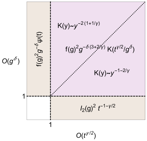
Figure 1 summarizes the different behaviors of p(g,t)𝑝𝑔𝑡p(g,t) in the plane (tγ/2,gδ)superscript𝑡𝛾2superscript𝑔𝛿(t^{\gamma/2},g^{\delta}) for a fast decreasing jump distribution and 0<γ<10𝛾10<\gamma<1. The ‘one-step’ (resp. ‘many-steps’) regime is on the left (resp. right) of the diagonal.
Refer to caption
Figure 1: Schematic representation of the asymptotic behaviors of p(g,t)𝑝𝑔𝑡p(g,t) for fast decreasing jump distributions and 0<γ<10𝛾10<\gamma<1 (amplitudes are given in the text). For t1much-greater-than𝑡1t\gg 1 and gO(1)less-than-or-similar-to𝑔𝑂1g\lesssim O(1), p(g,t)𝑝𝑔𝑡p(g,t) is given by Eq. (28) with μ=2𝜇2\mu=2. For both t1much-greater-than𝑡1t\gg 1 and g1much-greater-than𝑔1g\gg 1, one has the scaling form (78) with K(y)𝐾𝑦K(y) respectively given by the first line of (79) if tγ/2gδmuch-less-thansuperscript𝑡𝛾2superscript𝑔𝛿t^{\gamma/2}\ll g^{\delta} and by the second line of (79) if tγ/2gδmuch-greater-thansuperscript𝑡𝛾2superscript𝑔𝛿t^{\gamma/2}\gg g^{\delta}. For tO(1)less-than-or-similar-to𝑡𝑂1t\lesssim O(1) and g1much-greater-than𝑔1g\gg 1, p(g,t)𝑝𝑔𝑡p(g,t) is given by Eq. (75).

VI Scaling form of the asymptotic behavior of 𝒑(𝒈,𝒕)𝒑𝒈𝒕\bm{p(g,t)} for a Lévy flight at large 𝒕𝒕\bm{t} and 𝒈𝒈\bm{g}

In the preceding section we have found that for a fast decreasing jump distribution and 0<γ<10𝛾10<\gamma<1, the asymptotic behavior of p(g,t)𝑝𝑔𝑡p(g,t) at large t𝑡t and g𝑔g takes the scaling form (78). Here we consider a Lévy flight of index 0<μ<20𝜇20<\mu<2 corresponding to a slow decreasing jump distribution. We will see that, in this case too, p(g,t)𝑝𝑔𝑡p(g,t) at large t𝑡t and g𝑔g can be put into a scaling form for all 0<γ10𝛾10<\gamma\leq 1.

Consider first the case γ=1𝛾1\gamma=1. By Eq. (23) and the scaling form (87) in MMS2014 , p(g,t)𝑝𝑔𝑡p(g,t) depends on t𝑡t through the combination tgμ𝑡superscript𝑔𝜇tg^{-\mu} only as both t𝑡t and g𝑔g are large. Now, for 0<γ<10𝛾10<\gamma<1, the comparison of Eqs. (22) and (25) indicates that t𝑡t should be replaced with tγsuperscript𝑡𝛾t^{\gamma}. Thus, for 0<γ10𝛾10<\gamma\leq 1, p(g,t)𝑝𝑔𝑡p(g,t) is expected to depend on t𝑡t through the combination tγgμsuperscript𝑡𝛾superscript𝑔𝜇t^{\gamma}g^{-\mu} only as both t𝑡t and g𝑔g are large. The simplest scaling ansatz for p(g,t)𝑝𝑔𝑡p(g,t) consistent with this argument and the asymptotic behaviors (50) and (58) reads

p(g,t)1aτc(ag)1+μ(1+1/γ)Fμ,γ(aμtγgμτcγ)(g+andt+),similar-to𝑝𝑔𝑡1𝑎subscript𝜏𝑐superscript𝑎𝑔1𝜇11𝛾subscript𝐹𝜇𝛾superscript𝑎𝜇superscript𝑡𝛾superscript𝑔𝜇superscriptsubscript𝜏𝑐𝛾𝑔and𝑡p(g,t)\sim\frac{1}{a\tau_{c}}\,\left(\frac{a}{g}\right)^{1+\mu(1+1/\gamma)}F_{\mu,\,\gamma}\left(\frac{a^{\mu}t^{\gamma}}{g^{\mu}\tau_{c}^{\gamma}}\right)\ \ \ \ (g\rightarrow+\infty\ {\rm and}\ t\rightarrow+\infty), (87)

with the following large and small argument behaviors for the scaling function:

Fμ,γ(y){𝒞Iy1/μ1/γ,1Int(γ)<μ<2,𝒞IIy11/γlny,μ=1,𝒞IIIy11/γ,0<μ<1,(y+),similar-tosubscript𝐹𝜇𝛾𝑦casessubscript𝒞Isuperscript𝑦1𝜇1𝛾1Int𝛾𝜇2subscript𝒞IIsuperscript𝑦11𝛾𝑦𝜇1subscript𝒞IIIsuperscript𝑦11𝛾0𝜇1𝑦F_{\mu,\,\gamma}(y)\sim\left\{\begin{array}[]{ll}\mathcal{C}_{\rm I}\,y^{-1/\mu-1/\gamma},&1-{\rm Int}(\gamma)<\mu<2,\\ \mathcal{C}_{\rm II}\,y^{-1-1/\gamma}\ln y,&\mu=1,\\ \mathcal{C}_{\rm III}\,y^{-1-1/\gamma},&0<\mu<1,\end{array}\right.\ \ \ \ (y\rightarrow+\infty), (88)

and

Fμ,γ(y)𝒞IVy1/21/γ,(y0).similar-tosubscript𝐹𝜇𝛾𝑦subscript𝒞IVsuperscript𝑦121𝛾𝑦0F_{\mu,\,\gamma}(y)\sim\mathcal{C}_{\rm IV}\,y^{1/2-1/\gamma},\ \ \ \ (y\rightarrow 0). (89)

The term Int(γ)Int𝛾{\rm Int}(\gamma) in the first line of (88) denotes the integer part of γ𝛾\gamma and the last two lines are for 0<γ<10𝛾10<\gamma<1 only. The scaling form (87) holds in the regime where both g𝑔g and t𝑡t are large, with tγgμsuperscript𝑡𝛾superscript𝑔𝜇t^{\gamma}g^{-\mu} fixed.

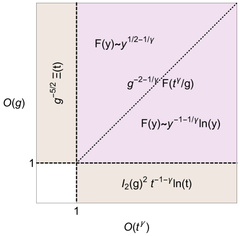
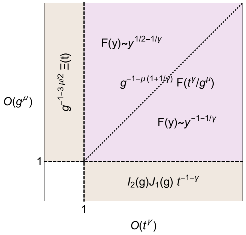
Figures 23, and 4 summarize the different behaviors of p(g,t)𝑝𝑔𝑡p(g,t) in the plane (tγ,gμ)superscript𝑡𝛾superscript𝑔𝜇(t^{\gamma},g^{\mu}) for a a Lévy flight of index 0<μ<20𝜇20<\mu<2. They correspond respectively to the cases 1Int(γ)<μ<21Int𝛾𝜇21-{\rm Int}(\gamma)<\mu<2 with 0<γ10𝛾10<\gamma\leq 1, μ=1𝜇1\mu=1 with 0<γ<10𝛾10<\gamma<1 and 0<μ<10𝜇10<\mu<1 with 0<γ<10𝛾10<\gamma<1.

Refer to caption
Figure 2: Schematic representation of the asymptotic behaviors of p(g,t)𝑝𝑔𝑡p(g,t) for a Lévy flight of index 1Int(γ)<μ<21Int𝛾𝜇21-{\rm Int}(\gamma)<\mu<2 and 0<γ10𝛾10<\gamma\leq 1 (amplitudes are given in the text). For t1much-greater-than𝑡1t\gg 1 and gO(1)less-than-or-similar-to𝑔𝑂1g\lesssim O(1), p(g,t)𝑝𝑔𝑡p(g,t) is given by the first line of Eq. (39). For both t1much-greater-than𝑡1t\gg 1 and g1much-greater-than𝑔1g\gg 1, one has the scaling form (87) with F(y)𝐹𝑦F(y) given by the first line of (88) if tγgμmuch-greater-thansuperscript𝑡𝛾superscript𝑔𝜇t^{\gamma}\gg g^{\mu} and by (89) if tγgμmuch-less-thansuperscript𝑡𝛾superscript𝑔𝜇t^{\gamma}\ll g^{\mu}. For tO(1)less-than-or-similar-to𝑡𝑂1t\lesssim O(1) and g1much-greater-than𝑔1g\gg 1, p(g,t)𝑝𝑔𝑡p(g,t) is given by Eq. (57).

Refer to caption
Figure 3: Schematic representation of the asymptotic behaviors of p(g,t)𝑝𝑔𝑡p(g,t) for a Lévy flight of index μ=1𝜇1\mu=1 and 0<γ<10𝛾10<\gamma<1 (amplitudes are given in the text). For t1much-greater-than𝑡1t\gg 1 and gO(1)less-than-or-similar-to𝑔𝑂1g\lesssim O(1), p(g,t)𝑝𝑔𝑡p(g,t) is given by the second line of Eq. (39). For both t1much-greater-than𝑡1t\gg 1 and g1much-greater-than𝑔1g\gg 1, one has the scaling form (87) with F(y)𝐹𝑦F(y) given by the second line of (88) if tγgmuch-greater-thansuperscript𝑡𝛾𝑔t^{\gamma}\gg g and by (89) if tγgmuch-less-thansuperscript𝑡𝛾𝑔t^{\gamma}\ll g. For tO(1)less-than-or-similar-to𝑡𝑂1t\lesssim O(1) and g1much-greater-than𝑔1g\gg 1, p(g,t)𝑝𝑔𝑡p(g,t) is given by Eq. (57) with μ=1𝜇1\mu=1.

Refer to caption
Figure 4: Schematic representation of the asymptotic behaviors of p(g,t)𝑝𝑔𝑡p(g,t) for a Lévy flight of index 0<μ<10𝜇10<\mu<1 and 0<γ<10𝛾10<\gamma<1 (amplitudes are given in the text). For t1much-greater-than𝑡1t\gg 1 and gO(1)less-than-or-similar-to𝑔𝑂1g\lesssim O(1), p(g,t)𝑝𝑔𝑡p(g,t) is given by the third line of Eq. (39). For both t1much-greater-than𝑡1t\gg 1 and g1much-greater-than𝑔1g\gg 1, one has the scaling form (87) with F(y)𝐹𝑦F(y) given by the third line of (88) if tγgμmuch-greater-thansuperscript𝑡𝛾superscript𝑔𝜇t^{\gamma}\gg g^{\mu} and by (89) if tγgμmuch-less-thansuperscript𝑡𝛾superscript𝑔𝜇t^{\gamma}\ll g^{\mu}. For tO(1)less-than-or-similar-to𝑡𝑂1t\lesssim O(1) and g1much-greater-than𝑔1g\gg 1, p(g,t)𝑝𝑔𝑡p(g,t) is given by Eq. (57).

VII Large 𝒕𝒕\bm{t} behavior of the marginal distribution 𝒑𝐭𝐢𝐦𝐞(𝒕)subscript𝒑𝐭𝐢𝐦𝐞𝒕\bm{p_{\rm time}(t)}

We can now determine the large t𝑡t behavior of the marginal distribution ptime(t)subscript𝑝time𝑡p_{\rm time}(t) of the time between the first two maxima. The marginal distribution pgap(g)subscript𝑝gap𝑔p_{\rm gap}(g) of the gap between the first two maxima does not depend on γ𝛾\gamma and is the same as the one already studied in Sec. 3 of Ref. MMS2014 in the discrete time RW setting.

VII.1 𝜸=𝟏𝜸1\bm{\gamma=1}

For γ=1𝛾1\gamma=1, the large t𝑡t behavior of ptime(t)subscript𝑝time𝑡p_{\rm time}(t) is readily obtained by integrating (23) over g𝑔g and by using the large l𝑙l asymptotics (112) in MMS2014 . One finds

ptime(t)1τc×{𝒜I(t/τc)11/μ,1<μ2,𝒜IIln(t/τc)(t/τc)2,μ=1,𝒜III(t/τc)2,0<μ<1,(t+),similar-tosubscript𝑝time𝑡1subscript𝜏𝑐casessubscript𝒜Isuperscript𝑡subscript𝜏𝑐11𝜇1𝜇2subscript𝒜II𝑡subscript𝜏𝑐superscript𝑡subscript𝜏𝑐2𝜇1subscript𝒜IIIsuperscript𝑡subscript𝜏𝑐20𝜇1𝑡p_{\rm time}(t)\sim\frac{1}{\tau_{c}}\times\left\{\begin{array}[]{ll}\mathcal{A}_{\rm I}\,(t/\tau_{c})^{-1-1/\mu},&1<\mu\leq 2,\\ \mathcal{A}_{\rm II}\,\ln(t/\tau_{c})\,(t/\tau_{c})^{-2},&\mu=1,\\ \mathcal{A}_{\rm III}\,(t/\tau_{c})^{-2},&0<\mu<1,\end{array}\right.\ \ \ \ (t\rightarrow+\infty), (90)

with

𝒜I=(πa)1Γ(1+1/μ)0+I2(g)2𝑑g,𝒜II=π2,𝒜III=μ10+yFμ, 1(y)𝑑y.subscript𝒜Isuperscript𝜋𝑎1Γ11𝜇superscriptsubscript0subscript𝐼2superscript𝑔2differential-d𝑔subscript𝒜IIsuperscript𝜋2subscript𝒜IIIsuperscript𝜇1superscriptsubscript0𝑦subscript𝐹𝜇1𝑦differential-d𝑦\begin{array}[]{l}\mathcal{A}_{\rm I}=(\pi a)^{-1}\Gamma(1+1/\mu)\,\int_{0}^{+\infty}I_{2}(g)^{2}dg,\\ \mathcal{A}_{\rm II}=\pi^{-2},\\ \mathcal{A}_{\rm III}=\mu^{-1}\int_{0}^{+\infty}yF_{\mu,\,1}(y)\,dy.\end{array} (91)

VII.2 𝟎<𝜸<𝟏0𝜸1\bm{0<\gamma<1}

To determine the large t𝑡t behavior of ptime(t)subscript𝑝time𝑡p_{\rm time}(t) for 0<γ<10𝛾10<\gamma<1, fix Λ11much-greater-thansubscriptΛ11\Lambda_{1}\gg 1, Λ2=O(1)subscriptΛ2𝑂1\Lambda_{2}=O(1), and for t>(Λ1/Λ2)μ/γ𝑡superscriptsubscriptΛ1subscriptΛ2𝜇𝛾t>(\Lambda_{1}/\Lambda_{2})^{\mu/\gamma} write

ptime(t)=0+p(g,t)𝑑g=0Λ1p(g,t)𝑑g+Λ1Λ2tγ/μp(g,t)𝑑g+Λ2tγ/μ+p(g,t)𝑑g.subscript𝑝time𝑡superscriptsubscript0𝑝𝑔𝑡differential-d𝑔superscriptsubscript0subscriptΛ1𝑝𝑔𝑡differential-d𝑔superscriptsubscriptsubscriptΛ1subscriptΛ2superscript𝑡𝛾𝜇𝑝𝑔𝑡differential-d𝑔superscriptsubscriptsubscriptΛ2superscript𝑡𝛾𝜇𝑝𝑔𝑡differential-d𝑔p_{\rm time}(t)=\int_{0}^{+\infty}p(g,t)\,dg=\int_{0}^{\Lambda_{1}}p(g,t)\,dg+\int_{\Lambda_{1}}^{\Lambda_{2}t^{\gamma/\mu}}p(g,t)\,dg+\int_{\Lambda_{2}t^{\gamma/\mu}}^{+\infty}p(g,t)\,dg. (92)

For 1<μ21𝜇21<\mu\leq 2 and t+𝑡t\rightarrow+\infty, (92) is dominated by the first two integrals in which one can use the large t𝑡t expression (28) of p(g,t)𝑝𝑔𝑡p(g,t). One finds

ptime(t)subscript𝑝time𝑡\displaystyle p_{\rm time}(t) similar-to\displaystyle\sim sin(πγ/μ)sin(π/μ)Γ(1+γ/μ)πaτc(t/τc)1+γ/μ0Λ2tγ/μI2(g)2𝑑g𝜋𝛾𝜇𝜋𝜇Γ1𝛾𝜇𝜋𝑎subscript𝜏𝑐superscript𝑡subscript𝜏𝑐1𝛾𝜇superscriptsubscript0subscriptΛ2superscript𝑡𝛾𝜇subscript𝐼2superscript𝑔2differential-d𝑔\displaystyle\frac{\sin(\pi\gamma/\mu)}{\sin(\pi/\mu)}\,\frac{\Gamma(1+\gamma/\mu)}{\pi a\tau_{c}\,(t/\tau_{c})^{1+\gamma/\mu}}\,\int_{0}^{\Lambda_{2}t^{\gamma/\mu}}I_{2}(g)^{2}dg (93)
similar-to\displaystyle\sim sin(πγ/μ)sin(π/μ)Γ(1+γ/μ)πaτc(t/τc)1+γ/μ0+I2(g)2𝑑g(t+).𝜋𝛾𝜇𝜋𝜇Γ1𝛾𝜇𝜋𝑎subscript𝜏𝑐superscript𝑡subscript𝜏𝑐1𝛾𝜇superscriptsubscript0subscript𝐼2superscript𝑔2differential-d𝑔𝑡\displaystyle\frac{\sin(\pi\gamma/\mu)}{\sin(\pi/\mu)}\,\frac{\Gamma(1+\gamma/\mu)}{\pi a\tau_{c}\,(t/\tau_{c})^{1+\gamma/\mu}}\,\int_{0}^{+\infty}I_{2}(g)^{2}dg\ \ \ \ (t\rightarrow+\infty).

For 0<μ<10𝜇10<\mu<1 and t+𝑡t\rightarrow+\infty, (92) is dominated by the contribution of large, O(tγ/μ)𝑂superscript𝑡𝛾𝜇O(t^{\gamma/\mu}), values of g𝑔g, i.e. by the last two integrals in which one can use the large t𝑡t and g𝑔g scaling form (87) of p(g,t)𝑝𝑔𝑡p(g,t). One gets

ptime(t)subscript𝑝time𝑡\displaystyle p_{\rm time}(t) similar-to\displaystyle\sim 1aτcΛ1+(ag)1+μ(1+1/γ)Fμ,γ(aμtγgμτcγ)𝑑g1𝑎subscript𝜏𝑐superscriptsubscriptsubscriptΛ1superscript𝑎𝑔1𝜇11𝛾subscript𝐹𝜇𝛾superscript𝑎𝜇superscript𝑡𝛾superscript𝑔𝜇superscriptsubscript𝜏𝑐𝛾differential-d𝑔\displaystyle\frac{1}{a\tau_{c}}\,\int_{\Lambda_{1}}^{+\infty}\left(\frac{a}{g}\right)^{1+\mu(1+1/\gamma)}F_{\mu,\,\gamma}\left(\frac{a^{\mu}t^{\gamma}}{g^{\mu}\tau_{c}^{\gamma}}\right)\,dg (94)
=\displaystyle= 1μτc1(t/τc)1+γ0aμtγ/Λ1μτcγy1/γFμ,γ(y)𝑑g1𝜇subscript𝜏𝑐1superscript𝑡subscript𝜏𝑐1𝛾superscriptsubscript0superscript𝑎𝜇superscript𝑡𝛾superscriptsubscriptΛ1𝜇superscriptsubscript𝜏𝑐𝛾superscript𝑦1𝛾subscript𝐹𝜇𝛾𝑦differential-d𝑔\displaystyle\frac{1}{\mu\tau_{c}}\,\frac{1}{(t/\tau_{c})^{1+\gamma}}\,\int_{0}^{a^{\mu}t^{\gamma}/\Lambda_{1}^{\mu}\tau_{c}^{\gamma}}y^{1/\gamma}F_{\mu,\,\gamma}(y)\,dg
similar-to\displaystyle\sim γ𝒞IIIμτcln(t/τc)(t/τc)1+γ(t+).𝛾subscript𝒞III𝜇subscript𝜏𝑐𝑡subscript𝜏𝑐superscript𝑡subscript𝜏𝑐1𝛾𝑡\displaystyle\frac{\gamma\mathcal{C}_{\rm III}}{\mu\tau_{c}}\,\frac{\ln(t/\tau_{c})}{(t/\tau_{c})^{1+\gamma}}\ \ \ \ (t\rightarrow+\infty).

where we have made the change of variable y=aμtγ/gμτcγ𝑦superscript𝑎𝜇superscript𝑡𝛾superscript𝑔𝜇superscriptsubscript𝜏𝑐𝛾y=a^{\mu}t^{\gamma}/g^{\mu}\tau_{c}^{\gamma} and used the third line of (88).

Finally, for μ=1𝜇1\mu=1 and t+𝑡t\rightarrow+\infty we use the second line of (88) in the second line of (94) with μ=1𝜇1\mu=1, which gives

ptime(t)γ2𝒞II2τcln2(t/τc)(t/τc)1+γ(t+).similar-tosubscript𝑝time𝑡superscript𝛾2subscript𝒞II2subscript𝜏𝑐superscript2𝑡subscript𝜏𝑐superscript𝑡subscript𝜏𝑐1𝛾𝑡p_{\rm time}(t)\sim\frac{\gamma^{2}\mathcal{C}_{\rm II}}{2\tau_{c}}\,\frac{\ln^{2}(t/\tau_{c})}{(t/\tau_{c})^{1+\gamma}}\ \ \ \ (t\rightarrow+\infty). (95)

To summarize, for 0<γ<10𝛾10<\gamma<1 the large t𝑡t behavior of the marginal distribution ptime(t)subscript𝑝time𝑡p_{\rm time}(t) is given by

ptime(t)1τc×{𝒜I(t/τc)1γ/μ,1<μ2,𝒜IIln2(t/τc)(t/τc)1γ,μ=1,𝒜IIIln(t/τc)(t/τc)1γ,0<μ<1,(t+),similar-tosubscript𝑝time𝑡1subscript𝜏𝑐casessuperscriptsubscript𝒜Isuperscript𝑡subscript𝜏𝑐1𝛾𝜇1𝜇2superscriptsubscript𝒜IIsuperscript2𝑡subscript𝜏𝑐superscript𝑡subscript𝜏𝑐1𝛾𝜇1superscriptsubscript𝒜III𝑡subscript𝜏𝑐superscript𝑡subscript𝜏𝑐1𝛾0𝜇1𝑡p_{\rm time}(t)\sim\frac{1}{\tau_{c}}\times\left\{\begin{array}[]{ll}\mathcal{A}_{\rm I}^{\prime}\,(t/\tau_{c})^{-1-\gamma/\mu},&1<\mu\leq 2,\\ \mathcal{A}_{\rm II}^{\prime}\,\ln^{2}(t/\tau_{c})\,(t/\tau_{c})^{-1-\gamma},&\mu=1,\\ \mathcal{A}_{\rm III}^{\prime}\,\ln(t/\tau_{c})\,(t/\tau_{c})^{-1-\gamma},&0<\mu<1,\end{array}\right.\ \ \ \ (t\rightarrow+\infty), (96)

with

𝒜I=a1𝒞IΓ(1μ/2)20+I2(g)2𝑑g,𝒜II=γ2𝒞II/2,𝒜III=γ𝒞III/μ,superscriptsubscript𝒜Isuperscript𝑎1subscript𝒞IΓsuperscript1𝜇22superscriptsubscript0subscript𝐼2superscript𝑔2differential-d𝑔superscriptsubscript𝒜IIsuperscript𝛾2subscript𝒞II2superscriptsubscript𝒜III𝛾subscript𝒞III𝜇\begin{array}[]{l}\mathcal{A}_{\rm I}^{\prime}=a^{-1}\mathcal{C}_{\rm I}\Gamma(1-\mu/2)^{2}\int_{0}^{+\infty}I_{2}(g)^{2}dg,\\ \mathcal{A}_{\rm II}^{\prime}=\gamma^{2}\mathcal{C}_{\rm II}/2,\\ \mathcal{A}_{\rm III}^{\prime}=\gamma\mathcal{C}_{\rm III}/\mu,\end{array} (97)

where 𝒞I=IΓ(1μ/2)2subscript𝒞IsubscriptIΓsuperscript1𝜇22\mathcal{C}_{\rm I}=\mathcal{B}_{\rm I}\Gamma(1-\mu/2)^{-2}, 𝒞II=IIπ1subscript𝒞IIsubscriptIIsuperscript𝜋1\mathcal{C}_{\rm II}=\mathcal{B}_{\rm II}\pi^{-1}, and 𝒞III=IItan(μπ/2)/2subscript𝒞IIIsubscriptII𝜇𝜋22\mathcal{C}_{\rm III}=\mathcal{B}_{\rm II}\tan(\mu\pi/2)/2, the amplitudes IsubscriptI\mathcal{B}_{\rm I} and IIsubscriptII\mathcal{B}_{\rm II} being respectively given by (37) and (38).

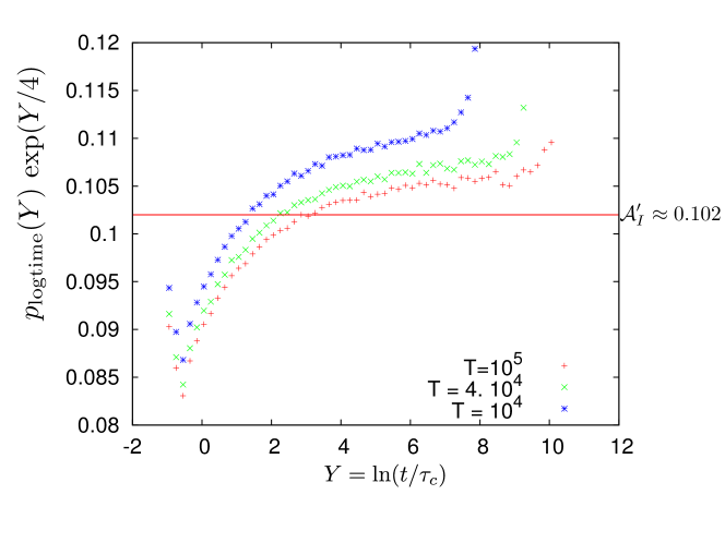
It can be seen that the smaller γ𝛾\gamma is, the slower ptime(t)subscript𝑝time𝑡p_{\rm time}(t) decreases as t𝑡t increases. The third lines of Eqs. (90) and (96) reveal an interesting freezing, as a function of μ𝜇\mu, of the large t𝑡t behavior of ptime(t)subscript𝑝time𝑡p_{\rm time}(t) as μ𝜇\mu decreases past the critical value μc=1subscript𝜇𝑐1\mu_{c}=1. It is the continuous time counterpart of the freezing phenomenon pointed out in Sec. 5 of MMS2014 for discrete time random walks. In particular, it follows immediately from (90) and (96) that the first moment of ptime(t)subscript𝑝time𝑡p_{\rm time}(t) is never defined. This means that although the typical size of t𝑡t is O(1)𝑂1O(1), its average always diverges with the total duration of the walk. Writing T𝑇T the total duration of the walk, Eqs. (90) and (96) yield the estimate

|t|{T1γ/μ1<μ2T1γ(lnT)2μ=1T1γlnT0<μ<1(T+),similar-todelimited-⟨⟩𝑡casessuperscript𝑇1𝛾𝜇1𝜇2superscript𝑇1𝛾superscript𝑇2𝜇1superscript𝑇1𝛾𝑇0𝜇1𝑇\langle|t|\rangle\sim\left\{\begin{array}[]{ll}T^{1-\gamma/\mu}&1<\mu\leq 2\\ T^{1-\gamma}(\ln T)^{2}&\mu=1\\ T^{1-\gamma}\ln T&0<\mu<1\end{array}\right.\ \ \ \ (T\rightarrow+\infty), (98)

for 0<γ10𝛾10<\gamma\leq 1.

VIII Numerical simulations

In this section, we check our main analytical results by comparing them with the ones of numerical simulations of the corresponding CTRW. In the simulations, the random jump variables ηisubscript𝜂𝑖\eta_{i}’s and the random time intervals between two successive jumps τisubscript𝜏𝑖\tau_{i}’s were drawn from the following distributions.

Jump variables. For μ=2𝜇2\mu=2, the jumps were drawn either from a Gaussian distribution f(η)=exp(η2/2)/2π𝑓𝜂superscript𝜂222𝜋f(\eta)=\exp(-\eta^{2}/2)/\sqrt{2\pi} – when we investigate the joint PDF of g𝑔g and t𝑡t for fast decreasing jump distribution – or from a symmetric exponential distribution f(η)=(b/2)exp(b|η|)𝑓𝜂𝑏2𝑏𝜂f(\eta)=(b/2)\exp{(-b|\eta|)} – when we study the marginal distribution ptime(t)subscript𝑝time𝑡p_{\rm time}(t) – in which case the amplitudes 𝒜Isubscript𝒜I{\cal A}_{\rm I} and 𝒜Isubscriptsuperscript𝒜I{\cal A^{\prime}}_{\rm I} in (11) and (12) can be evaluated exactly. On the other hand, for 0<μ<20𝜇20<\mu<2, we chose for f(η)𝑓𝜂f(\eta) a symmetric Pareto distribution of index μ𝜇\mu of the form

f(η)={0,for|η|<1μ2|η|1μ,for|η|1,𝑓𝜂casesotherwise0for𝜂1otherwise𝜇2superscript𝜂1𝜇for𝜂1\displaystyle f(\eta)=\begin{cases}&0\;,\;{\rm for}\;|\eta|<1\\ &\dfrac{\mu}{2}\,|\eta|^{-1-\mu}\;,\;{\rm for}\;|\eta|\geq 1\;,\end{cases} (99)

for which it is straightforward to compute the parameter a𝑎a in Eq. (2). One finds,

a=[Γ(1μ)cos(μπ2)]1/μ.𝑎superscriptdelimited-[]Γ1𝜇𝜇𝜋21𝜇\displaystyle a=\left[\Gamma(1-\mu)\cos{\left(\frac{\mu\pi}{2}\right)}\right]^{1/\mu}\;. (100)

The reason for such a choice is twofold: (i) random numbers drawn from (99) are easy and fast to generate numerically (see for instance Ref. MRS2013 ) and (ii) f(η)𝑓𝜂f(\eta) is a power law for all |η|1𝜂1|\eta|\geq 1 (instead of |η|1much-greater-than𝜂1|\eta|\gg 1 ) which allows us to access the asymptotic regime characterizing Lévy flights rather quickly in numerical simulations.

Time intervals. Similarly, to generate a CTRW numerically, it is also convenient to draw the time variables τisubscript𝜏𝑖\tau_{i}’s from a distribution Ψ(τ)Ψ𝜏\Psi(\tau) which is a (one-sided) Pareto distribution of index γ<1𝛾1\gamma<1 of the form

Ψ(τ)={0,forτ<1γτ1γ,forτ1.Ψ𝜏casesotherwise0for𝜏1otherwise𝛾superscript𝜏1𝛾for𝜏1\displaystyle\Psi(\tau)=\begin{cases}&0\;,\;{\rm for}\;\tau<1\\ &\gamma\,\tau^{-1-\gamma}\;,\;{\rm for}\;\tau\geq 1\;.\end{cases} (101)

For such a distribution the characteristic time τcsubscript𝜏𝑐\tau_{c} is given by

τc=[Γ(1γ)]1/γ.subscript𝜏𝑐superscriptdelimited-[]Γ1𝛾1𝛾\displaystyle\tau_{c}=[\Gamma(1-\gamma)]^{1/\gamma}\;. (102)

VIII.1 Scaling form of the asymptotic behavior of 𝒑(𝒈,𝒕)𝒑𝒈𝒕\bm{p(g,t)} at large 𝒕𝒕\bm{t} and 𝒈𝒈\bm{g}

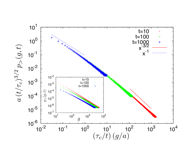
Computing a joint PDF numerically is notoriously a quite hard task. So, instead of p(g,t)𝑝𝑔𝑡p(g,t) we consider the cumulative distribution

p>(g,t)=tp(g,t)𝑑t,subscript𝑝𝑔𝑡superscriptsubscript𝑡𝑝𝑔superscript𝑡differential-dsuperscript𝑡\displaystyle p_{>}(g,t)=\int_{t}^{\infty}p(g,t^{\prime})dt^{\prime}\;, (103)

which yields better statistics at a lesser cost.

We first present the result for a fast decreasing jump distribution f(η)𝑓𝜂f(\eta) in the sense of Sec. V.3, i.e. f(η+x)f(η)exp(cηδx)similar-to𝑓𝜂𝑥𝑓𝜂𝑐superscript𝜂𝛿𝑥f(\eta+x)\sim f(\eta)\exp(-c\,\eta^{\delta}\,x) when η𝜂\eta\to\infty [see Eq. (68)]. In this case, one expects from Eq. (6) that in the limit t𝑡t\to\infty and g𝑔g\to\infty keeping gtγ/(2δ)𝑔superscript𝑡𝛾2𝛿g\,t^{-\gamma/(2\delta)} fixed, p>(g,t)subscript𝑝𝑔𝑡p_{>}(g,t) takes the following scaling form:

p>(g,t)af(g)2(tτc)3γ/2H((ac)1/δg(t/τc)γ/(2δ)),similar-tosubscript𝑝𝑔𝑡𝑎𝑓superscript𝑔2superscript𝑡subscript𝜏𝑐3𝛾2𝐻superscript𝑎𝑐1𝛿𝑔superscript𝑡subscript𝜏𝑐𝛾2𝛿\displaystyle p_{>}(g,t)\sim a\,f(g)^{2}\left(\frac{t}{\tau_{c}}\right)^{-3\gamma/2}H\left(\frac{(a\,c)^{1/\delta}g}{(t/\tau_{c})^{\gamma/(2\delta)}}\right)\;,\; (104)

where the scaling function H(z)𝐻𝑧H(z) is related to the scaling function K(z)𝐾𝑧K(z) through the relation

H(z)=1z3δ1/z2δ/γK(yγ/2)𝑑y.𝐻𝑧1superscript𝑧3𝛿subscript1superscript𝑧2𝛿𝛾𝐾superscript𝑦𝛾2differential-d𝑦\displaystyle H(z)=\frac{1}{z^{3\delta}}\int_{1/z^{2\delta/\gamma}}K(y^{\gamma/2})\,dy\;. (105)

From the asymptotic behaviors of K(z)𝐾𝑧K(z) in Eq. (7), one deduces the asymptotic behaviors of H(z)𝐻𝑧H(z) as follows

H(z){2DIIγz2δ,(z0)DIγzδ(z).similar-to𝐻𝑧casesotherwise2subscript𝐷II𝛾superscript𝑧2𝛿𝑧0otherwisesubscript𝐷I𝛾superscript𝑧𝛿𝑧\displaystyle H(z)\sim\begin{cases}&\dfrac{2\,D_{\rm II}}{\gamma}\;z^{-2\delta}\;,\;(z\to 0)\\ &\dfrac{D_{\rm I}}{\gamma}\;z^{-\delta}\;\;(z\to\infty)\;.\end{cases} (106)

As discussed above, the limit z𝑧z\to\infty corresponds to the ‘single-step’ regime while the limit z0𝑧0z\to 0 corresponds to the ‘many-steps’ regime.

In Fig. 5 we show a plot of (t/τc)3γ/2p>(g)[f(g)]2superscript𝑡subscript𝜏𝑐3𝛾2subscript𝑝𝑔superscriptdelimited-[]𝑓𝑔2(t/\tau_{c})^{3\gamma/2}p_{>}(g)[f(g)]^{2} as a function of (ac)1/δ(t/τc)γ/(2δ)gsuperscript𝑎𝑐1𝛿superscript𝑡subscript𝜏𝑐𝛾2𝛿𝑔(a\,c)^{1/\delta}(t/\tau_{c})^{-\gamma/(2\delta)}g for a fast decreasing jump distribution, namely a Gaussian jump distribution, corresponding to δ=1𝛿1\delta=1, and with γ=0.9𝛾0.9\gamma=0.9, for different values of t=5000,10000,20000𝑡50001000020000t=5000,10000,20000 and 400004000040000, while the total duration of the CTRW is T=105𝑇superscript105T=10^{5}. The data have been obtained by averaging over 106superscript10610^{6} independent realizations of the CTRW. We see on this plot that, for sufficiently large values of g𝑔g, the curves for different times t𝑡t tend to collapse on a master curve, as predicted by Eq. (104), which indeed holds only in the limit g𝑔g\to\infty, t𝑡t\to\infty with gtγ/(2δ)𝑔superscript𝑡𝛾2𝛿g\,t^{-\gamma/(2\delta)} fixed. For smaller values of g𝑔g we see a clear deviation from this scaling form. We emphasize on the fact that, in our simulations, we have been able to access the regime where the scaling variable gtγ/(2δ)proportional-toabsent𝑔superscript𝑡𝛾2𝛿\propto g\,t^{-\gamma/(2\delta)} is small (corresponding to the ‘many-steps’ regime), where H(z)𝐻𝑧H(z) is expected to behave as H(z)z2proportional-to𝐻𝑧superscript𝑧2H(z)\propto z^{-2}. It is extremely difficult to reach the complementary ‘single-step’ regime corresponding to gtγ/(2δ)1much-greater-than𝑔superscript𝑡𝛾2𝛿1g\,t^{-\gamma/(2\delta)}\gg 1. Indeed, for such high values of t5000𝑡5000t\geq 5000 the condition gtγ/(2δ)1much-greater-than𝑔superscript𝑡𝛾2𝛿1g\,t^{-\gamma/(2\delta)}\gg 1 with δ=1𝛿1\delta=1 and γ=0.9𝛾0.9\gamma=0.9 yields g46much-greater-than𝑔46g\gg 46, which is already large enough to prevent any access to reliable statistics (to understand the difficulty, just realize that for the Gaussian jump distribution we consider in the ‘single-step’ regime, the typical gaps are greater than 101010 less often than one time out of the Avogadro’s number). Consequently, the clear numerical observation of the crossover behavior between the ‘many-steps’ and the ‘single-step’ regimes described by the scaling function in Eq. (104) goes beyond the scope of the present paper. Notice that, for γ=1𝛾1\gamma=1 and tτcsimilar-to𝑡subscript𝜏𝑐t\sim\tau_{c}, the ‘single-step regime’ was clearly demonstrated in Ref. MMS2014 .
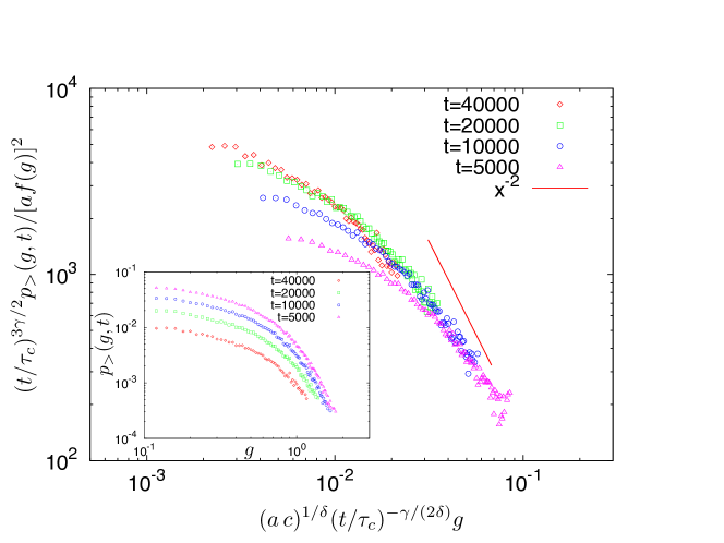
Refer to caption
Figure 5: Plot of (t/τc)3γ/2p>(g)[f(g)]2superscript𝑡subscript𝜏𝑐3𝛾2subscript𝑝𝑔superscriptdelimited-[]𝑓𝑔2(t/\tau_{c})^{3\gamma/2}p_{>}(g)[f(g)]^{2} as a function of (ac)1/δ(t/τc)γ/(2δ)gsuperscript𝑎𝑐1𝛿superscript𝑡subscript𝜏𝑐𝛾2𝛿𝑔(a\,c)^{1/\delta}(t/\tau_{c})^{-\gamma/(2\delta)}g for a fast decreasing jump distribution, namely a Gaussian jump distribution, corresponding to δ=1𝛿1\delta=1, and with γ=0.9𝛾0.9\gamma=0.9. The different curves correspond to different values of t=5000,10000,20000𝑡50001000020000t=5000,10000,20000 and 400004000040000 for a CTRW of duration T=105𝑇superscript105T=10^{5}. The (relatively) good collapse of the different curves for large values of g𝑔g corroborate the scaling form predicted in Eq. (104). The solid line is a guide to eyes, corresponding to the small argument behavior of the scaling function H(z)𝐻𝑧H(z) in Eq. (106) with δ=1𝛿1\delta=1. Inset: same data as in the main panel but without the rescaling.

We now present numerical results for Lévy flights (0<μ<20𝜇20<\mu<2), for which f(η)𝑓𝜂f(\eta) is slow decreasing in the sense of Sec. V.1. In this case, one expects from Eq. (8) that in the limit t𝑡t\to\infty and g𝑔g\to\infty at fixed gtγ/μ𝑔superscript𝑡𝛾𝜇gt^{-\gamma/\mu}, p>(g,t)subscript𝑝𝑔𝑡p_{>}(g,t) takes the following scaling form:

p>(g,t)1a(tτc)γ(1+1/μ)Gμ,γ(ga(τct)γ/μ),similar-tosubscript𝑝𝑔𝑡1𝑎superscript𝑡subscript𝜏𝑐𝛾11𝜇subscript𝐺𝜇𝛾𝑔𝑎superscriptsubscript𝜏𝑐𝑡𝛾𝜇\displaystyle p_{>}(g,t)\sim\frac{1}{a}\left(\frac{t}{\tau_{c}}\right)^{-\gamma(1+1/\mu)}G_{\mu,\gamma}\left(\frac{g}{a}\left(\frac{\tau_{c}}{t}\right)^{\gamma/\mu}\right)\;, (107)

where the function Gμ,γ(z)subscript𝐺𝜇𝛾𝑧G_{\mu,\gamma}(z) is related to the scaling function Fμ,γ(z)subscript𝐹𝜇𝛾𝑧F_{\mu,\gamma}(z) through the relation

Gμ,γ(z)=1z1+μ1/zμ/γFμ,γ(yγ)𝑑y.subscript𝐺𝜇𝛾𝑧1superscript𝑧1𝜇superscriptsubscript1superscript𝑧𝜇𝛾subscript𝐹𝜇𝛾superscript𝑦𝛾differential-d𝑦\displaystyle G_{\mu,\gamma}(z)=\frac{1}{z^{1+\mu}}\int_{1/z^{\mu/\gamma}}^{\infty}F_{\mu,\gamma}(y^{\gamma})\,dy\;. (108)

The small and large z𝑧z behaviors of Gγ,μ(z)subscript𝐺𝛾𝜇𝑧G_{\gamma,\mu}(z) are readily obtained from the asymptotic behaviors of Fμ,γ(z)subscript𝐹𝜇𝛾𝑧F_{\mu,\gamma}(z) given in Eqs. (9) and (10). One gets

Gμ,γ(z)𝒞IIIz1+μ(z),similar-tosubscript𝐺𝜇𝛾𝑧subscriptsuperscript𝒞IIIsuperscript𝑧1𝜇𝑧\displaystyle G_{\mu,\gamma}(z)\sim\frac{{\cal C}^{\prime}_{\rm III}}{z^{1+\mu}}\;\;(z\to\infty)\;, (109)

for large z𝑧z, where 𝒞III=0Fμ,γ(yγ)𝑑ysubscriptsuperscript𝒞IIIsuperscriptsubscript0subscript𝐹𝜇𝛾superscript𝑦𝛾differential-d𝑦{\cal C}^{\prime}_{\rm III}=\int_{0}^{\infty}F_{\mu,\gamma}(y^{\gamma})\,dy, and

Gμ,γ(z){𝒞Izμ, 1Int(γ)<μ<2𝒞IIγz1ln(1/z),μ=1𝒞IIIz1, 0<μ<1.(z0),similar-tosubscript𝐺𝜇𝛾𝑧casesotherwisesubscript𝒞Isuperscript𝑧𝜇1Int𝛾𝜇2otherwisesubscript𝒞II𝛾superscript𝑧11𝑧𝜇1otherwisesubscript𝒞IIIsuperscript𝑧1 0𝜇1𝑧0\displaystyle G_{\mu,\gamma}(z)\sim\begin{cases}&{{\cal C}_{\rm I}}\,{z^{-\mu}}\;,\;1-{\rm Int}(\gamma)<\mu<2\\ &\dfrac{{\cal C}_{\rm II}}{\gamma}z^{-1}\ln(1/z)\;,\;\mu=1\\ &{{\cal C}_{\rm III}}\,{z^{-1}}\;,\;0<\mu<1\;.\end{cases}\hfill\;(z\to 0)\;, (110)

for small z𝑧z, where the last two lines are for 0<γ<10𝛾10<\gamma<1 only.

Refer to caption
Figure 6: Plot of a(t/τc)γ(1+1/μ)p>(g,t)𝑎superscript𝑡subscript𝜏𝑐𝛾11𝜇subscript𝑝𝑔𝑡a\,(t/\tau_{c})^{\gamma(1+1/\mu)}\,p_{>}(g,t) as a function of (g/a)(τc/t)γ/μ𝑔𝑎superscriptsubscript𝜏𝑐𝑡𝛾𝜇(g/a)({\tau_{c}}/{t})^{\gamma/\mu} with γ=μ=1/2𝛾𝜇12\gamma=\mu=1/2 for different values of t=10,100𝑡10100t=10,100 and t=1000𝑡1000t=1000, for a CTRW of total duration T=104𝑇superscript104T=10^{4}. The good collapse of the curves for different values of t𝑡t confirm the scaling form predicted in Eq. (107). The dashed and solid lines are guides to the eyes, indicating the algebraic behaviors predicted in Eqs. (109) and (110). Inset: same data as in the main panel but without the rescaling.

In Fig. 6 we show a scaled plot of a(t/τc)γ(1+1/μ)p>(g,t)𝑎superscript𝑡subscript𝜏𝑐𝛾11𝜇subscript𝑝𝑔𝑡a\,(t/\tau_{c})^{\gamma(1+1/\mu)}\,p_{>}(g,t) as a function of (g/a)(τc/t)γ/μ𝑔𝑎superscriptsubscript𝜏𝑐𝑡𝛾𝜇(g/a)({\tau_{c}}/{t})^{\gamma/\mu} with γ=μ=1/2𝛾𝜇12\gamma=\mu=1/2 for different values of t=10,100𝑡10100t=10,100 and t=1000𝑡1000t=1000, for CTRWs of total duration T=104𝑇superscript104T=10^{4}. The data have been obtained by averaging over 106superscript10610^{6} independent realizations of the CTRW. This plot demonstrates a good agreement with our predictions for the scaling form of the joint PDF in Eq. (107) as well as with the asymptotic behaviors predicted in Eqs. (109) and (110).

VIII.2 Asymptotic behavior of 𝒑𝐭𝐢𝐦𝐞(𝒕)subscript𝒑𝐭𝐢𝐦𝐞𝒕\bm{p_{\rm time}(t)} at large 𝒕𝒕\bm{t}

An interesting feature of our results for the distribution ptime(t)subscript𝑝time𝑡p_{\rm time}(t) of the time t𝑡t between the first two maxima is the presence of logarithmic corrections for 0<μ10𝜇10<\mu\leq 1 and 0<γ<10𝛾10<\gamma<1 [see Eq. (12)]. To demonstrate these logarithmic corrections numerically, it is convenient to study the distribution plogtime(Y)subscript𝑝logtime𝑌p_{\rm logtime}(Y) of the logarithm of the time, Y=ln(t/τc)𝑌𝑡subscript𝜏𝑐Y=\ln(t/\tau_{c}) instead of the time distribution itself. From plogtime(Y)=τceYptime(τceY)subscript𝑝logtime𝑌subscript𝜏𝑐superscripte𝑌subscript𝑝timesubscript𝜏𝑐superscripte𝑌p_{\rm logtime}(Y)=\tau_{c}{\rm e}^{Y}p_{\rm time}(\tau_{c}{\rm e}^{Y}) and Eq. (12) it follows that the asymptotic behavior of plogtime(Y)subscript𝑝logtime𝑌p_{\rm logtime}(Y) at large Y𝑌Y and for 0<γ<10𝛾10<\gamma<1 is given by

plogtime(Y){𝒜Iexp(γμY), 1<μ2𝒜IIY2exp(γY),μ=1𝒜IIIYexp(γY),0<μ<1,similar-tosubscript𝑝logtime𝑌casesotherwisesubscriptsuperscript𝒜I𝛾𝜇𝑌1𝜇2otherwisesubscriptsuperscript𝒜IIsuperscript𝑌2𝛾𝑌𝜇1otherwisesubscriptsuperscript𝒜III𝑌𝛾𝑌0𝜇1\displaystyle p_{\rm logtime}(Y)\sim\begin{cases}&{\cal A}^{\prime}_{\rm I}\,\exp{\left(-\dfrac{\gamma}{\mu}\,Y\right)}\;,\;1<\mu\leq 2\\ &{\cal A}^{\prime}_{\rm II}\,Y^{2}\,\exp{\left(-\gamma\,Y\right)}\;,\,\mu=1\\ &{\cal A}^{\prime}_{\rm III}\,Y\exp{\left(-\gamma\,Y\right)}\;,0<\mu<1\;,\end{cases} (111)

with the amplitudes

𝒜I=12πsin(γπ/2)Γ(1+γ/2)subscriptsuperscript𝒜I12𝜋𝛾𝜋2Γ1𝛾2\displaystyle{\cal A}^{\prime}_{\rm I}=\frac{1}{2\pi}{\sin{\left({\gamma\pi}/{2}\right)}\Gamma(1+{\gamma}/{2})} (112)
𝒜II=γ22π3Γ(1+γ)sin(γπ),subscriptsuperscript𝒜IIsuperscript𝛾22superscript𝜋3Γ1𝛾𝛾𝜋\displaystyle{\cal A}^{\prime}_{\rm II}=\frac{\gamma^{2}}{2\pi^{3}}\Gamma(1+\gamma)\sin{(\gamma\pi)}\;, (113)
𝒜III=γ2μπ2tan(μπ2)sin(γπ)Γ(1+γ),subscriptsuperscript𝒜III𝛾2𝜇superscript𝜋2𝜇𝜋2𝛾𝜋Γ1𝛾\displaystyle{\cal A}^{\prime}_{\rm III}=\frac{\gamma}{2\mu\pi^{2}}\tan{\left(\frac{\mu\pi}{2}\right)}\sin{(\gamma\pi)}\Gamma(1+\gamma)\;, (114)

where the value of 𝒜Isubscriptsuperscript𝒜I{\cal A}^{\prime}_{\rm I} corresponds to a symmetric exponential jump distribution (see the beginning of this section).
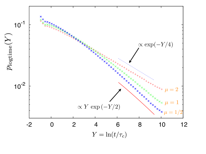
Refer to caption
Figure 7: Plot of plogtime(Y)subscript𝑝logtime𝑌p_{\rm logtime}(Y) as a function of Y=ln(t/τc)𝑌𝑡subscript𝜏𝑐Y=\ln(t/\tau_{c}) on a log-linear plot for γ=1/2𝛾12\gamma=1/2 and for different values of μ=2,1𝜇21\mu=2,1 and 1/2121/2, corresponding to the three different regimes in Eq. (111). The solid lines are guides to the eyes corresponding to the asymptotic behaviors for μ=2𝜇2\mu=2 and μ=1/2𝜇12\mu=1/2 given in Eq. (111). These data have been obtained for CTRWs of length T=105𝑇superscript105T=10^{5}.
Refer to caption
Figure 8: Plot of plogtime(Y)exp(γY/μ)subscript𝑝logtime𝑌𝛾𝑌𝜇p_{\rm logtime}(Y)\,\exp(\gamma Y/\mu) for γ=1/2𝛾12\gamma=1/2 and μ=2𝜇2\mu=2 (namely exponentially distributed jumps) as a function of Y=log(t/τc)𝑌𝑡subscript𝜏𝑐Y=\log(t/\tau_{c}) for CTRWs of increasing length, namely T=104𝑇superscript104T=10^{4}, T=4104𝑇4superscript104T=4\,\cdot 10^{4} and T=105𝑇superscript105T=10^{5}. Note that the upward bending is a finite size effect, as our predictions actually hold for 1tTmuch-less-than1𝑡much-less-than𝑇1\ll t\ll T which is confirmed by the fact that this bending happens for larger and larger values of t𝑡t as the total duration T𝑇T of the CTRW increases. In the appropriate regime such that 1tTmuch-less-than1𝑡much-less-than𝑇1\ll t\ll T plogtime(Y)exp(γY/μ)subscript𝑝logtime𝑌𝛾𝑌𝜇p_{\rm logtime}(Y)\,\exp(\gamma Y/\mu) converges to a constant which is indeed close (with an accuracy of less than 5%percent\% for T=105𝑇superscript105T=10^{5}) to our analytical predictions 𝒜Isubscriptsuperscript𝒜I{\cal A}^{\prime}_{\rm I} in Eq. (111).

In Fig. 7, we show a plot of plogtime(Y)subscript𝑝logtime𝑌p_{\rm logtime}(Y) as a function of Y𝑌Y for three different values of μ𝜇\mu: μ=2𝜇2\mu=2 (with exponentially distributed jumps), μ=1𝜇1\mu=1, and μ=1/2𝜇12\mu=1/2, that are representative of the three different regimes in Eq. (111), for a fixed value of γ=1/2𝛾12\gamma=1/2. This plot shows that the large Y𝑌Y behavior of plogtime(Y)subscript𝑝logtime𝑌p_{\rm logtime}(Y) does depend on μ𝜇\mu as predicted in Eq. (111). To make a precise comparison between our numerical results and our analytical predictions (and in particular to demonstrate the expected logarithmic corrections), we now analyze these data, for different values of μ𝜇\mu, more carefully.

Fig. 8 corresponds to the case of a sub-diffusive walk with μ=2𝜇2\mu=2 (with exponentially distributed jumps) and γ=1/2𝛾12\gamma=1/2. We show a plot of plogtime(Y)exp(γY/μ)subscript𝑝logtime𝑌𝛾𝑌𝜇p_{\rm logtime}(Y)\,\exp(\gamma Y/\mu) for γ=1/2𝛾12\gamma=1/2 as a function of Y=log(t/τc)𝑌𝑡subscript𝜏𝑐Y=\log(t/\tau_{c}) for CTRWs of increasing length, namely T=104𝑇superscript104T=10^{4}, T=4 104𝑇superscript4104T=4\,10^{4} and T=105𝑇superscript105T=10^{5}. Here, the data have again been obtained by averaging over 106superscript10610^{6} independent CTRWs. It can be seen that in the time interval 1tTmuch-less-than1𝑡much-less-than𝑇1\ll t\ll T where our prediction actually holds, plogtime(Y)exp(γY/μ)subscript𝑝logtime𝑌𝛾𝑌𝜇p_{\rm logtime}(Y)\,\exp(\gamma Y/\mu) approaches a constant which gets closer to the expected value 𝒜Isubscriptsuperscript𝒜I{\cal A}^{\prime}_{\rm I} as the total duration T𝑇T of the walk increases. The observed small upward discrepancy, as well as the steep upward bending for larger Y𝑌Y, are finite size effects. Note the very stretched vertical scale. For the longest walks with T=105𝑇superscript105T=10^{5}, numerical and analytical results are in agreement to within an accuracy of less than 5%percent\%.

Refer to caption
Figure 9: Plot of plogtime(Y)exp(γY)subscript𝑝logtime𝑌𝛾𝑌p_{\rm logtime}(Y)\exp{(\gamma Y)} as a function of Y𝑌Y for μ=1/2𝜇12\mu=1/2 and γ=1/2𝛾12\gamma=1/2 and for different durations of the CTRW: T=104𝑇superscript104T=10^{4}, T=4104𝑇4superscript104T=4\,\cdot 10^{4}, and T=105𝑇superscript105T=10^{5}. The solid line, which corresponds to our analytical result in Eq. (111) with 𝒜III=0.0448968subscriptsuperscript𝒜III0.0448968{\cal A}^{\prime}_{\rm III}=0.0448968\ldots is a guide to eye, indicating a good agreement between our analytical results and numerics. This linear behavior is a clear signature of the logarithmic corrections in ptime(t)subscript𝑝time𝑡p_{\rm time}(t), which is a peculiarity of the CTRW model. Upward bending at large Y𝑌Y is a finite size effect which decreases as T𝑇T increases.
Refer to caption
Figure 10: Plot of plogtime(Y)exp(γY)subscript𝑝logtime𝑌𝛾𝑌p_{\rm logtime}(Y)\exp{(\gamma Y)} as a function of Y𝑌Y for μ=1𝜇1\mu=1 and γ=1/2𝛾12\gamma=1/2 and for different durations of the CTRW, T=104𝑇superscript104T=10^{4}, T=4104𝑇4superscript104T=4\,\cdot 10^{4}, and T=105𝑇superscript105T=10^{5}. The solid line, which corresponds to our analytical result in Eq. (111) with 𝒜II=0.000357277subscriptsuperscript𝒜II0.000357277{\cal A}^{\prime}_{\rm II}=0.000357277\ldots is a guide to eye, indicating a good agreement between our analytical results and numerics. Upward bending at large Y𝑌Y is a finite size effect which decreases as T𝑇T increases.

Next we consider the case μ=1/2𝜇12\mu=1/2, which corresponds to the third regime in Eq. (111). In Fig. 9 we show a plot of plogtime(Y)exp(γY)subscript𝑝logtime𝑌𝛾𝑌p_{\rm logtime}(Y)\,\exp{(\gamma\,Y)}, for μ=1/2𝜇12\mu=1/2 and γ=1/2𝛾12\gamma=1/2 as a function of Y𝑌Y and for different durations of the CTRW, T=104𝑇superscript104T=10^{4}, T=4104𝑇4superscript104T=4\,\cdot 10^{4}, and T=105𝑇superscript105T=10^{5}. As before, the data have been obtained by averaging over 106superscript10610^{6} independent CTRWs. The linear behavior, in a good agreement with our analytical prediction 𝒜IIIYproportional-toabsentsubscriptsuperscript𝒜III𝑌\propto{\cal A}^{\prime}_{\rm III}\,Y, is a clear signature of the logarithmic correction of ptime(t)subscript𝑝time𝑡p_{\rm time}(t) as expected from our analytical result in Eq. (12).

Finally, Fig. 10 shows a plot of plogtime(Y)exp(γY)subscript𝑝logtime𝑌𝛾𝑌p_{\rm logtime}(Y)\exp{(\gamma Y)} as a function of Y𝑌Y, for μ=1𝜇1\mu=1, γ=1/2𝛾12\gamma=1/2, and the same walk durations as before (averaging procedure is also the same). It can be seen that our numerical data are compatible with the expected quadratic behavior (111), plogtime(Y)exp(γY)𝒜IIY2similar-tosubscript𝑝logtime𝑌𝛾𝑌subscriptsuperscript𝒜IIsuperscript𝑌2p_{\rm logtime}(Y)\exp{(\gamma Y)}\sim{\cal A}^{\prime}_{\rm II}\,Y^{2}. Recalling that Y=log(t/τc)𝑌𝑡subscript𝜏𝑐Y=\log(t/\tau_{c}), this quadratic behavior confirms our analytical predictions for ptime(t)subscript𝑝time𝑡p_{\rm time}(t) in Eq. (12).

IX Summary and perspectives

In this paper, we have performed a detailed analytical study of the statistics of the gap g𝑔g and the time interval t𝑡t between the first two maxima of a CTRW in the limit where the number of steps in the walk goes to infinity. The results we have obtained are quite general as we have addressed the question for the wide class of a symmetric, bounded, and (piecewise) continuous jump distribution, including the case of Lévy flights of index μ𝜇\mu, with 0<μ<20𝜇20<\mu<2. The average trapping time τdelimited-⟨⟩𝜏\langle\tau\rangle between two successive jumps can be either finite, τ=τc<+delimited-⟨⟩𝜏subscript𝜏𝑐\langle\tau\rangle=\tau_{c}<+\infty, or infinite. In the latter case, the trapping time distribution Ψ(τ)Ψ𝜏\Psi(\tau) is assumed to have a power law tail Ψ(τ)τ1γproportional-toΨ𝜏superscript𝜏1𝛾\Psi(\tau)\propto\tau^{-1-\gamma}, with 0<γ<10𝛾10<\gamma<1.

For a finite average trapping time between two successive jumps, our results coincide with the ones in MMS2014 , devoted to discrete time RWs, in which the number of jumps between the first two maxima, l𝑙l, is merely replaced with t/τc𝑡subscript𝜏𝑐t/\tau_{c}, as expected from simple law of large number arguments. On the other hand, our study provides a non trivial extension of the one in MMS2014 to the case where the average time between two successive jumps does not exist and law of large number arguments cannot be used. In particular, by taking γ<μ/2𝛾𝜇2\gamma<\mu/2 it makes it possible to address the question for sub-diffusive RWs, out of reach of the discrete time analysis of MMS2014 .

We have first shown that the joint PDF pn(g,t)subscript𝑝𝑛𝑔𝑡p_{n}(g,t) converges to a stationary PDF, pn(g,t)p(g,t)subscript𝑝𝑛𝑔𝑡𝑝𝑔𝑡p_{n}(g,t)\rightarrow p(g,t), as n𝑛n\to\infty, where n𝑛n is the total number of steps in the walk. We have then obtained an explicit expression of the Laplace transform of p(g,t)𝑝𝑔𝑡p(g,t) w.r.t. t𝑡t, given in equations (20) and (17), from which we have performed a detailed analysis of p(g,t)𝑝𝑔𝑡p(g,t) in the plane (g,t)𝑔𝑡(g,t) for μ𝜇\mu and γ𝛾\gamma in the whole ranges 0<μ20𝜇20<\mu\leq 2 and 0<γ10𝛾10<\gamma\leq 1, and for the three different main classes identified in MMS2014 : (i) slow, (ii) exponentially, and (iii) fast decreasing f(η)𝑓𝜂f(\eta) at large η𝜂\eta.

In the case (iii) of a fast decreasing jump distribution (μ=2𝜇2\mu=2) with 0<γ<10𝛾10<\gamma<1 and in the scaling regime g,t1much-greater-than𝑔𝑡1g,\ t\gg 1 with fixed tγ/2gμsuperscript𝑡𝛾2superscript𝑔𝜇t^{\gamma/2}g^{-\mu}, we have shown that p(g,t)𝑝𝑔𝑡p(g,t) takes a scaling form, Eqs. (6) and (7). The switch from the first to the second behavior (7) corresponds to the cross-over from a ‘concentration’ – or ‘one-step’ – regime where the walker get stuck for a long time t𝑡t at the second maximum and then jumps directly to the first maximum, to a ‘many-steps’ regime where she/he travels a long walk of total duration t𝑡t (with many steps) between the second and the first maxima. We have summarized these results in Figure 1. The numerical observation of the cross-over and ‘one-step’ regime is still out of reach as it requires a prohibitively large value of g𝑔g. Note, however, that we expect a similar scaling form for p(g,t)𝑝𝑔𝑡p(g,t) if f(η)𝑓𝜂f(\eta) has a bounded support ηmaxηηmaxsubscript𝜂max𝜂subscript𝜂max-\eta_{\rm max}\leq\eta\leq\eta_{\rm max} and g+𝑔g\rightarrow+\infty is replaced with gηmax𝑔subscript𝜂maxg\rightarrow\eta_{\rm max}, the largest possible (bounded) value of the gap. This should make a numerical observation of the cross-over and ‘one-step’ regime easier in this case. The study of p(g,t)𝑝𝑔𝑡p(g,t) for jump distributions with a bounded support (in both discrete and continuous time settings) will be the subject of a future work.

For type (i) Lévy flights of index μ𝜇\mu, with 0<μ<20𝜇20<\mu<2, and in the scaling regime g,t1much-greater-than𝑔𝑡1g,\ t\gg 1 with fixed tγgμsuperscript𝑡𝛾superscript𝑔𝜇t^{\gamma}g^{-\mu}, we have shown that p(g,t)𝑝𝑔𝑡p(g,t) takes the scaling form (8) with the asymptotic behaviors (9) and (10). These results, summarized in Figures 2 to 4, provide a non trivial extension of the ones in MMS2014 to the case 0<γ<10𝛾10<\gamma<1.

Finally, from the stationary joint PDF p(g,t)𝑝𝑔𝑡p(g,t) we have computed the stationary marginal distribution, ptime(t)subscript𝑝time𝑡p_{\rm time}(t), of the time between the first to maxima of the walk. Its asymptotic behavior, which depends on γ𝛾\gamma and the Lévy index μ𝜇\mu, is summarized in equations (11), (12), and in Table 1. The third lines of (11) and (12) reveal that the freezing phenomenon of the large t𝑡t behavior of ptime(t)subscript𝑝time𝑡p_{\rm time}(t), as a function of μ𝜇\mu, as μ𝜇\mu decreases past the value μc=1subscript𝜇𝑐1\mu_{c}=1, which was first put in evidence for discrete time RWs in MMS2013 ; MMS2014 , also exists for CTRWs. As a consequence, the first moment of ptime(t)subscript𝑝time𝑡p_{\rm time}(t) is never defined.

Our study raises interesting open questions. For instance, this work focuses on the first gap and it would be interesting to study higher order gaps. In Ref. SM2012 , the study of the k𝑘k-th gap of long random walks, for μ=2𝜇2\mu=2 revealed a rich and universal behavior (i.e., independent of the jump distribution) of the stationary PDF of the k𝑘k-th gap in the large k𝑘k limit. The extension of these results, which also hold for CTRW with μ=2𝜇2\mu=2 and any value of 0<γ10𝛾10<\gamma\leq 1, to Lévy flights, i.e. 0<μ<20𝜇20<\mu<2, remains a challenging open question. Similarly, it would very interesting to study the time between the k𝑘k-th and (k+1)𝑘1(k+1)-th maximum for CTRW (both for γ=1𝛾1\gamma=1 and γ<1𝛾1\gamma<1), for which one also expects universality for k1much-greater-than𝑘1k\gg 1. Finally, the generalization of our results to higher dimensions would also be very interesting.

References

  • (1) Comtet, A., Majumdar, S. N.: Precise asymptotics for a random walker’s maximum. J. Stat. Mech. P06013 (2005).
  • (2) Derrida, B., Brunet E.: Statistics at the tip of a branching random walk and the delay of traveling waves, EPL 87 60010 (2009).
  • (3) Derrida, B., Brunet E.: A branching random walk seen from the tip, J. Stat. Phys. 143, 420 (2011).
  • (4) Majumdar, S. N., Mounaix, Ph., Schehr, G.: Exact Statistics of the Gap and Time Interval Between the First Two Maxima of Random Walks, Phys. Rev. Lett. 111, 070601 (2013).
  • (5) Majumdar, S. N., Mounaix, Ph., Schehr, G.: On the gap and time interval between the first two maxima of long random walks. J. Stat. Mech. P09013 (2014).
  • (6) Schehr, G., Le Doussal, P.: Extreme value statistics from the Real Space Renormalization Group: Brownian Motion, Bessel Processes and Continuous Time Random Walks, J. Stat. Mech. P01009 (2010).
  • (7) Bouchaud, J.-P., Mézard M.: Universality classes for extreme-value statistics, J. Phys. A 30, 7997 (1997).
  • (8) Dean D. S. , Majumdar S. N.: Extreme Value Statistics of Hierarchically Correlated Variables: Deviation from Gumbel Statistics and Anomalous Persistence, Phys. Rev. E 64, 046121 (2001).
  • (9) Pollaczek F.: Fonctions caractéristiques de certaines répartitions définies au moyen de la notion d’ordre, C. R. Acad. Sci. Paris 234, 2334 (1952).
  • (10) Spitzer F.: A combinatorial lemma and its application to probability theory, Trans. Am. Math. Soc. 82, 323 (1956).
  • (11) Schehr, G., Majumdar, S. N., Universal Order Statistics of Random Walks, Phys. Rev. Lett. 108, 040601 (2012).
  • (12) Scher, H., Montroll, E. W., Anomalous transit-time dispersion in amorphous solids, Phys. Rev. B 12, 2455 (1975).
  • (13) Bouchaud J. P., Georges A., Anomalous diffusion in disordered media: Statistical mechanisms, models and physical applications, Phys. Rep. 195, 127 (1990).
  • (14) Metzler, K., Klafter, I., The random walk’s guide to anomalous diffusion: a fractional dynamics approach, Phys. Rep. 339, 1 (2000).
  • (15) Carmi, S., Turgeman, L., Barkai, E., On distributions of functionals of anomalous diffusion paths, J. Stat. Phys. 141, 1071 (2010).
  • (16) Franke, J., Majumdar, S. N., Survival probability of an immobile target surrounded by mobile traps, J. Stat. Mech. P05024 (2012).
  • (17) De Mulatier C., Rosso A., Schehr G., Asymmetric Lévy flights in the presence of absorbing boundaries J. Stat. Mech. P10006 (2013).