Nonlocal effects and counter measures in cascading failures

Abstract

We study the propagation of cascading failures in complex supply networks with a focus on nonlocal effects occurring far away from the initial failure. It is shown that a high clustering and a small average path length of a network generally suppress nonlocal overloads. These properties are typical for many real-world networks, often called small-world networks, such that cascades propagate mostly locally in these networks. Furthermore, we analyze the spatial aspects of countermeasures based on the intentional removal of additional edges. Nonlocal actions are generally required in networks which have a low redundancy and are thus especially vulnerable to cascades.

I Introduction

A reliable supply of electric power fundamentally underlies the function of most of our technical infrastructure and affects all aspects of daily life. Large-scale power outages can thus have potentially catastrophic consequences and cause huge economic losses Fair04 ; Amin05a . Therefore it is an important goal to understand the vulnerability of a grid on all scales in order to secure our energy supply. A promising direction is to combine methods and models of power engineering with the recent progress in the theory of complex networks Hill06 ; Newm11 ; Bara12 ; Brum13 .

Notably, most large-scale outages can be traced back to the failure of a single transmission element of our power supply system Pour06 . The initial failure then causes secondary failures in other elements of the grid and eventually a global cascade. Cascading failures have been analyzed in a variety of studies from the viewpoint of mathematics and theoretical physics in the last decade Watt02 ; Mott02 ; Buld10 ; Albe04 ; Zhao04 ; Cruc04b ; Heid08 ; Simo08 ; Schn11 ; Mott04 ; Scha06 ; Huan08 . It has been analyzed which structural properties of networks promote or prevent global cascades Mott02 ; Watt02 ; Albe04 ; Zhao04 ; Cruc04b ; Buld10 and how fluctuations and transient dynamics affect the vulnerability of the grid Heid08 ; Simo08 . Different countermeasures were discussed in order to make a grid more robust beforehand Schn11 or to stop a cascade before it affects major parts of the grid Mott04 ; Scha06 ; Huan08 .

Most of these studies adopt a global perspective on cascading failures and focus on the statistical properties of the cascade and potential countermeasures. In this article we study cascades from a more microscopic perspective and analyze the location and propagation of failures. In particular, we characterize the nonlocality of secondary failures and show which structural features determine the nonlocality during the propagation of a cascade. It is shown that overloads occur mostly locally, i.e. in the immediate neighborhood of the failing element, when the network is strongly clustered and ‘small’. Remarkably, these two features are found for many real-world networks in technology as well as in biology and sociology Watt98 . We then extend these ideas to analyze the mechanism and the spatial aspects of countermeasures based on the intentional shutdown of transmission elements Mott04 ; Huan08 .

II Models for cascading failures

To analyze the spatial aspects of cascading failures in complex networks we use a model introduced by Motter and Lai in Mott02 ; Mott04 . Related models were introduced and discussed in Holm02a ; Holm02b ; Cruc04 . The Motter-Lai model assumes that at each time step, one unit of energy or information is sent from each vertex to each other vertex in the connected component along the shortest path. The load of each edge $F_{ij}$ is then given by the number of shortest paths running over this edge $i\leftrightarrow j$, which is nothing than the edge betweenness centrality Newm10 . Furthermore, it is assumed that the capacity of each edge is proportional to the load of the edge in the initial intact network,

$$K_{ij}=(1+\alpha)F^{(0)}_{ij}\,,$$ (1)

where the superscript $(0)$ denotes the initial intact network. The tolerance parameter $\alpha\geq 0$ quantifies the global redundancy of the network: Each edge can transmit $(1+\alpha)$ of its initial load before it becomes overloaded.

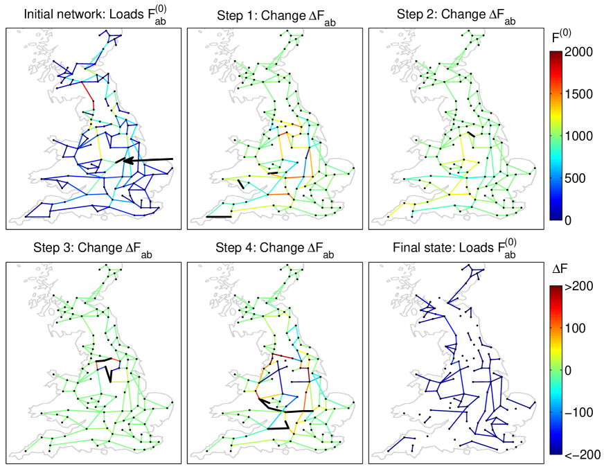
Figure 1: (Color online) Propagation of a cascade of failures in the British high-voltage power transmission grid. The cascade is triggered by a single edge which drops out of operation (marked by an arrow). As a consequence, the network flow is rerouted which causes overloads of further edges which also break down (thick black lines). Most interestingly, the overloads do not occur in the immediate neighborhood of the removed edge. The network structure was taken from Simo08 ; 12powergrid and the tolerance parameter is $\alpha=0.5$.

Then it is analyzed what happens if one edge is damaged, such that it is effectively removed from the network. Obviously, the other edges have to take over the load such that $F_{ij}$ will generally increase. If the load exceeds the capacity of an edge $(i,j)$, $F_{ij}>K_{ij}$, then this edge becomes overloaded and also drops out of service, which causes a further redistribution of the flows and further overloads. This can trigger a large cascade of failures disconnecting the entire grid. We note that the original articles Mott02 ; Mott04 analyze potential overloads of vertices instead of edges. However, in cascading failures of power grids, usually the transmission lines (i.e. the edges) become overloaded and drop out of service. Therefore we concentrate on edges instead of vertices in the present paper.

An example of a cascading failure in the Motter-Lai model is shown in Fig. 1 for the topology of the British high-voltage transmission grid Simo08 ; 12powergrid . The cascade is triggered by the breakdown of one edge marked by an arrow in the upper left panel of the figure. The cascade then propagates through the network and finally leads to a state where the network is decomposed into several components.

A remarkable aspect of this example is that the cascade is strongly nonlocal. The distance of the defective edge causing the flow redistribution and the overloaded edges is rather large. Therefore a local perspective is not sufficient to evaluate the effects of the breakdown of single edges in a complex network. In the following we will analyze the spatial aspects of cascading failures in detail and show which topologies are especially prone to nonlocal failures.

On a global scale, the damage caused by a cascading failure is generally quantified by the number of vertices which are still connected when the cascade comes to a halt. To be precise, we measure the number of vertices in the largest connected component in the final state (called $G$) as well as in the initial network (called $G_{0}$). A high value of the ratio $G/G_{0}$ indicates that the network is still mostly intact, while a low value value of $G/G_{0}$ indicates a fatal global cascade. Numerical results for the average effect of cascading failures are shown in Fig. 2 (a,b) as a function of the tolerance parameter $\alpha$. Obviously the size of the final cluster $G/G_{0}$ increases with $\alpha$ – in general, catastrophic global cascades are more likely in networks that lack redundancy, i.e. for low values of $\alpha$. This plot also shows which amount of redundancy is needed in order to contain the possible effects to a maximum acceptable value. How the network topology determines these curves and thus the global robustness of a network has been discussed intensively in the literature (see, e.g., Mott02 ; Watt02 ; Albe04 ; Zhao04 ; Cruc04b ; Buld10 ). However, such an analysis does not reveal which parts of the network are prone to outage and how a cascade propagates on a microscopic level.

III Nonlocality of cascading failures

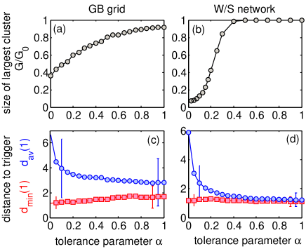
Figure 2: (Color online) Resilience and nonlocality in cascading failures as a function of the tolerance parameter $\alpha$. (a,b) Relative size of the largest connected cluster after the cascade $G/G_{0}$, averaging over all possible trigger edges. (c,d) Average of the distance to the trigger edge for all overloaded edges ($d_{\rm av}(1)$, $\circ$) and for the edge which is nearest to the trigger ($d_{\rm min}(1)$, $\square$) for the first step of the cascade. The vertical bars show typical values for the respective standard deviation. Results are collected for all possible trigger edges in the respective network: (a,c) the British power grid Simo08 ; 12powergrid and (b,d) a W/S network with $N=500$ vertices, $k=4$ and $q=0.2$ Watt98 .

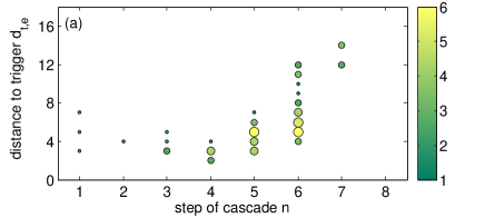
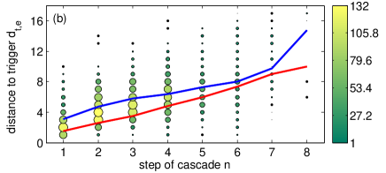
Figure 3: (Color online) Propagation of a cascade of failures in the British high-voltage power transmission grid. The color color and the area of the symbols indicates the number of edges that are overloaded at step $n$ and located at a distance $d_{t,e}$ from the trigger edge. (a) Data for a single cascade as shown in Fig. 1. (b) Data collected for all possible trigger edges in the same network. The blue line is the average distance to the trigger $d_{\rm av}(n)$ and the red line is distance of the nearest overloaded edge $d_{\rm min}(n)$.

To analyze the nonlocality of failures in complex networks we must first specify the meaning of ‘distance’ in a network. The distance $d_{a,b}$ of two vertices $a$ and $b$ is defined as as the number of edges in a shortest path connecting them Jung12 . Furthermore we need the distance of two edges $(a,b)$ and $(c,d)$, which is defined as the number of vertices on a shortest path between the edges such that

$$d_{(a,b),(c,d)}=\min_{x\in\{a,b\},y\in\{c,d\}}d_{x,y}+1.$$ (2)

In the following we denote by $t$ the edge whose initial break- down triggers the cascade and by $\text{ov}(n)$ the set of all edges overloaded at the nth step of the cascade. We then analyze the distribution of the distances $d_{t,e}$ for all overloaded edges $e\in\text{ov}(n)$ as well as its average

$$d_{\rm av}(n)=\Big{\langle}\big{\langle}d_{t,e}\big{\rangle}_{e\in\text{ov}(n)}\Big{\rangle}_{t}\,.$$ (3)

Furthermore, we analyze where the nearest overload occurs during the $n$th step, i.e the minimum of the distance between the trigger $t$ and all edges $e\in\text{ov}(n)$. This quantity is calculated separately for each cascade and we take the average over all potential trigger edges,

$$d_{\rm min}(n)=\Big{\langle}\min_{e\in\text{ov}(n)}d_{t,e}\Big{\rangle}_{t}\,.$$ (4)

The distance between overloaded edges and the initial trigger edge is shown in Fig. 3 (a) for the example shown in Fig. 1. Already in the first step $n=1$ we observe three overloaded edges at distances $d=3,5,7$, i.e. at rather remote locations. In the following we will concentrate on this first step of the cascade which facilitates the understanding of nonlocal effects. In later steps $n>1$ of the cascade there are generally multiple failures occurring at once. Further outages then occur due to the collective redistribution of network flows and cannot be attributed to a single cause alone. Quantifying the direct nonlocality of flow rerouting, i.e the nonlocality from one step of a cascade to the next step, thus faces conceptual difficulties except for step $n=1$. The distance of overloaded edges to the initial trigger edge shown in Fig. 3 accounts for the indirect nonlocality of a cascade for $n>1$, as it includes the propagation over several intermediate steps.

The influence of the global redundancy of a network on the nonlocality of flow rerouting is analyzed in Figure 2 (c,d). We plot the distance between the overloaded edges and the trigger edge $d_{\rm av}(n)$ and $d_{\rm min}(n)$ for $n=1$ (the direct nonlocality) as a function of the tolerance parameter $\alpha$. The first quantity shows where typical overloads occurs, while the latter quantity shows where the nearest overload occurs. It is observed that the average distance between overload and trigger $d_{\rm av}(1)$ decreases strongly as a function of the tolerance parameter $\alpha$. In highly redundant networks, i.e. for large values of $\alpha$, a large change of the flow $F_{i,j}$ is needed to induce an overload. Such changes are rare and occur almost exclusively in the neighborhood of the trigger. The average distance between trigger and overload $d_{\rm av}(1)$ is small and the rare cascades propagate ’locally’. In weakly redundant networks, i.e. for small value of $\alpha$, already medium scale changes of the flow $F_{i,j}$ induce overloads. Such changes occur frequently also in remote areas of the network. The average distance to the trigger $d_{\rm av}(1)$ is large and cascades can be strongly nonlocal. Such events are hard to predict and to contain.

IV The role of network topology

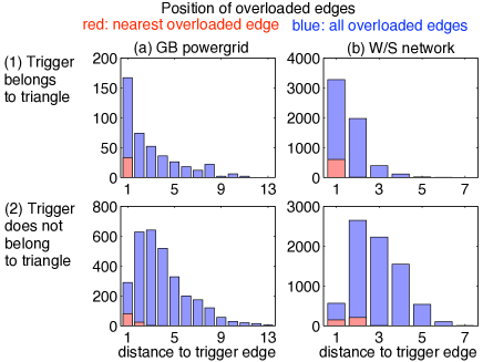
Figure 4: (Color online) The position of overloaded edges after the failure of a single trigger edge strongly depends on whether the trigger belongs to a triangle (upper panels) or not (lower panels). We plot a histogram of the distances to the trigger edge for all overloaded edges ($d_{t,e}$ for all $e\in\text{ov}(1)$, blue) and for the edge which is nearest to the trigger ($\min_{e\in\text{ov}(1)}d_{t,e}$, red). Results are collected for all possible trigger edges in the respective network: (a) the British power grid with $\alpha=0.1$ Simo08 ; 12powergrid , (c) a W/S network with $N=500$ vertices, $k=4$, $q=0.2$ and $\alpha=0.1$ Watt98 .

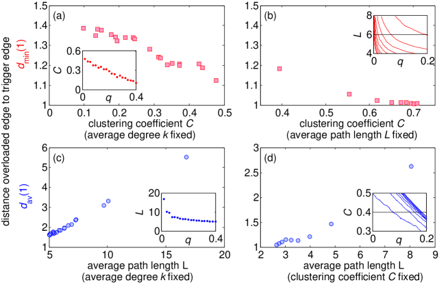
Figure 5: (Color online) Nonlocality as a function of the network topology. (a,b) The average distance of the nearest overloaded edge to the trigger $d_{\rm min}(1)$ decreases with the clustering coefficient $C$ of the network. (c,d) The average distance of all overloaded edges $d_{\rm av}(1)$ increases with the average path length $L$. In panels (a,c) results are shown for W/S networks with fixed average degree $k=4$ and different values of the topological randomness $q$. The insets show how $C$ and $L$ scale with $q$. In panels (b,d) results are shown for W/S networks with different degrees $k=4,6,\ldots,20$. The topological randomness $q$ has been chosen such that either the path length is fixed as $L\approx 6$ in (b) or the clustering coefficient is fixed as $C\approx 0.4$ in (d), cf. the insets. The network has $N=500$ nodes and $\alpha=0.2$.

The network topology has a decisive influence on the collective dynamics of complex networks, in particular the spread of information or perturbations (see Stro01 ; Bocc06 ; Newm10 and references therein). The nonlocality of cascades of failures is essentially determined by two topological features of the grid: (1) the size of the network which is measured by the average shortest path length

$$L:=\langle d_{x,y}\rangle_{x,y}$$ (5)

where the average is taken over all pairs of nodes $x,y$ and (2) the availability of short redundant pathways in the network. Such short paths are especially available if the trigger edge belongs to a triangle footnote . On a global scale the presence of triangles in the network is quantified by the clustering coefficient Watt98

$$C:=\frac{3\times\mbox{number of triangles}}{\mbox{number of connected triplets of vertices}}\,.$$ (6)

These conclusions hold for individual cascades in a given network (cf. Fig. 4) and for average cascades in networks with variable topology (cf. Fig. 5).

We first consider individual cascades for a given network topology in more detail. When a single trigger edge $(a,b)$ breaks down, the flow $F_{a,b}$ has to be rerouted via an alternative path in the network. This may cause an overload and thus a secondary failure at another edge $(i,j)$. Such an overload can happen locally, i.e. in the direct neighborhood of the trigger edge defined by $d_{(a,b),(i,j)}=1$ but also at a remote location in the network. The location of potential overloads is determined by the location of the alternative paths which take over the load. In particular, a short alternative path is available when the vertices $a$ and $b$ belong to a closed triangle $(a,b,c)$ footnote . Then there is an alternative path of length $2$ given by $a-c-b$, which will take over most of the flow $F_{a,b}$ when the edge $(a,b)$ fails. In this case it is very likely that an overload occurs locally at the two edges $(a,c)$ and $(c,b)$.

A statistical analysis of individual cascades confirms this claim. Figure 4 shows histogram of the distance between the overloaded edges and the trigger edge, where we distinguish if the trigger belongs to a triangle or not. Results are shown for all overloads as well as for the nearest overload. If the trigger edge belongs to a triangle (upper panels), the nearest overload occurs almost always within the triangle, i.e. at a distance of one. Further overloads can occur at different positions, but the probability decreases strongly with the distance. On the contrary, nonlocal overloads are much more frequent if the trigger edge does not belong to a triangle (lower panels). The highest number of overloads is found not in the immediate neighborhood of the trigger edge but at distance of $d=2$ or $d=3$. In this case the redistribution of the flow $F_{ab}$ cannot be predicted within a simple local picture.

To analyze how global structural properties of a network determine the nonlocality of cascading failures we simulate cascades for an ensemble of networks that interpolate between regular and random structures introduced by Watts and Strogatz Watt98 , which are referred to as W/S networks in the following. To generate such a network one starts with a ring, where each of the $N$ vertices is connected to its $k$ neighbors, $k$ being the average degree of the network. The total number of edges in the network is thus given by $Nk/2$. Then a fraction $q$ of all edges is randomly selected, deleted and re-inserted at a random position in the network. To reveal the influence of the size $L$ and the clustering coefficient $C$ , we study two cases in detail: (1) W/S networks with a fixed value of $k$ and different topological randomness $q$, which affects both $C$ and $L$ simultaneously (Fig. 5 a, c) and (2) W/S networks where where either $C$ or $L$ is kept constant by varying $k$ and $q$ simultaneously (Fig. 5 b, d).

The position of the nearest overload is essentially determined by the clustering coefficient $C$ which measures the probability that the trigger edge belongs to a triangle. Indeed, we observe a strong decrease of the distance $d_{\rm min}(1)$ with increasing clustering coefficient $C$ (cf. figure 5 (a,b)). This holds regardless of the fact whether we keep the degree $k$ or the average path length $L$ fixed.

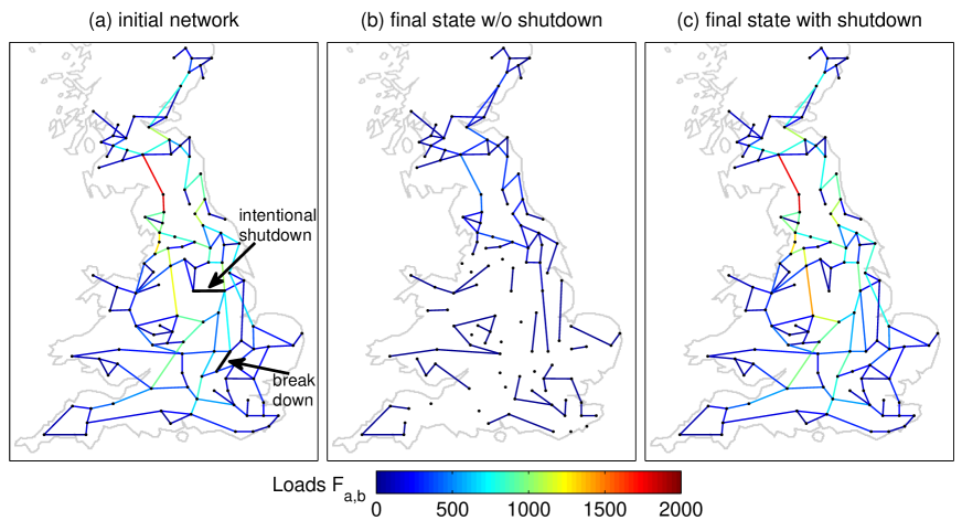
Figure 6: (Color online) Preventing a cascading failure by the intentional removal of a second edge within the Motter-Lai model. (a) We consider a scenario where one edge breaks down. As a counter measure a second carefully selected edge is shut down. The two edges are marked by arrows. (b) Without any counter measure the initial breakdown triggers a cascade of failures fragmenting the network. (c) The cascade can be completely prevented if a second, carefully chosen edge is also shut down (intentional removal, IR). When the two marked edges are removed simultaneously, no cascade takes place and the network remains fully connected. The network structure was taken from Simo08 ; 12powergrid and the tolerance parameter is $\alpha=0.5$.

The size of a network $L$ obviously limits the distances of vertices and edges. The numerical results plotted in figure 5 (c,d) reveal a much stronger influence. The average distance of the overloaded edges to the trigger $d_{\rm av}(1)$ increases almost linearly with the average path length $L$. Only for very small values of $L$ does the distance saturate slightly below the lower limit $1$. This result holds regardless of the fact whether we keep the degree $k$ or the clustering coefficient $C$ fixed.

We conclude that nonlocal overloads are particularly likely if the network is weakly clustered and has a large average path length. Remarkably, many real-world networks from power grids to biological and social network are so-called small worlds in the sense that both the clustering is high and the average path length is low. This small-world regime is recovered in the W/S network ensemble for intermediate values of the topological randomness $q$ Watt98 . Our results suggest the conclusion that such small-world networks are particularly local in the sense that the probability for nonlocal failures is smallest. This result may provide an additional reason why many real-world network have small-world properties (cf. the discussion in Menc13 ).

V Preventing cascades by intentional removal

An effective counterstrategy for preventing global cascades of failures is the intentional removal (IR) of parts of the network Mott04 ; Huan08 . Similar actions are taken in real-world power grids in case of an emergency. If the power is no longer balanced in one part of the grid, for example after a cascade of transmission line failures, several consumers are actively disconnected (see, e.g., UCTE07 ). An example for a successful application of this strategy is shown in figure 6 where the removal of one additional edge prevents the cascade completely. A statistical analysis of the effectiveness of IR in the Motter/Lai-model is shown in Fig. 7 for a W/S network. We compare the effect of an optimized IR to cascades triggered by the breakdown of a single edge (called $N-1$ errors) and the uncorrelated simultaneous breakdown of two edges (called $N-2$ errors). Remarkably, IR can reduce the number of disconnected vertices by more than $50\%$ for intermediate values of the tolerance parameter $\alpha$.

Two basic mechanisms contribute to the effectiveness of intentional removal. First, a small part of the network can be intentionally disconnected by removing a single edge. This is possible if this part of the network is connected to the rest through a single edge only, which is then called a bridge Jung12 . In the Motter-Lai model each vertex transmits one unit of information or energy to all other vertices in the connected component. If several vertices are disconnected they do no longer send or receive information or energy from the rest such that the overall network flow decreases. This method can be used to limit the consequences to a small local outage instead of a global cascade. This can be very effective in practice, but in any case parts of the network become disconnected.

However, in many cases there are much more sophisticated methods to prevent or stop a cascade of failures. An example is shown in Fig. 6, where the breakdown of a single edge causes a cascade of failures leading to a strong fragmentation of the network. On the contrary, the intentional removal of another edge at a distance of $2$ prevents the cascade completely. In these cases the intentional removal of an edge leads to a collective redistribution of the network flows which is beneficial and improves network stability. We conclude that the removed edge is actually counterproductive as it degrades network stability. This is analog to Braess’ paradox, where the addition of new edges in a supply or traffic network worsens its operation or makes a network unstable Brae68 ; Nish10 ; 12braess ; 13nonlocal . Preventing cascades by intentional removal can thus be seen as an application of Braess’ paradox.

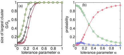
Figure 7: (Color online) Effectivity of intentional removal (IR) for preventing cascading failures as a function of the tolerance parameter $\alpha$. (a) Relative size of the largest connected cluster after the cascade $G/G_{0}$ averaging over all possible trigger edges. We compare cascades triggered by $N-1$ errors ($\circ$) and uncorrelated $N-2$ errors ($\diamond$) to the effect of an optimized intentional removal ($\square$). (b) Probability that IR leads to an increase of the final cluster size without disconnecting the network (green squares) in comparison to the probability that IR has no effect (red diamonds) and that IR disconnects the grid (blue circles). Results are collected for all possible trigger edges in a W/S network with $N=500$ vertices, $k=4$ and $q=0.2$ Watt98 .

The effectiveness of optimal IR is further analyzed in Fig. 7 (b) as a function of the tolerance parameter $\alpha$ for a W/S network. For a low value of the $\alpha$, IR is very effective in most cases and does not rely on the intentional disconnection of parts of the grid. For the given network topology, this holds for more than $90\%$ of all possible trigger edges. For high values of $\alpha$, most initial failures do not lead to a cascade at all. Consequently, IR has no effect with a very high probability – simply because it is not needed.

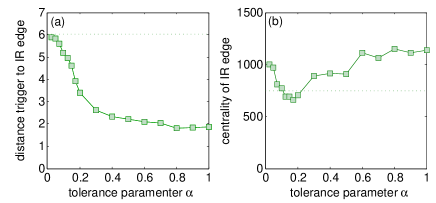
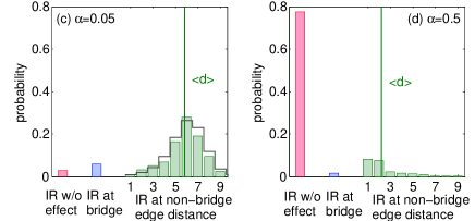
Figure 8: (Color online) Nonlocality of intentional removal for preventing cascading failures. (a) Average distance of the intentionally removed edge and the trigger edge as a function of the tolerance parameter $\alpha$. (b) Average betweenness centrality of the intentionally removed edge as a function of the tolerance parameter $\alpha$. In (a,b) we disregard cases where IR has no effect or disconnects the grid. The dashed line shows the average shortest path distance $L$ and the average centrality, respectively, for comparison. (c,d) Histogram of the distances of the intentionally removed edge and the trigger edge in case that IR leads to an increase of the final cluster size without disconnecting the network (green bars) for two values of $\alpha$ Grey lines show the distance distribution for all edges in the network for comparison. The red bars indicate the probability that that IR has no effect and the blue bars the probability that IR disconnects the grid. Results are averaged over all trigger edges for a W/S network with $N=500$, $k=4$ and $q=0.2$. The dashed lines

There is a further significant difference between networks with high and low redundancy, respectively. In Fig. 8 we analyze the characteristics of the intentionally removed edge which optimizes $G/G_{0}$. The betweenness centrality of the intentionally removed edges is higher than average, except for intermediate values of the parameter $\alpha$ (cf. Mott04 ). Similar results are found for the closeness centrality (not shown). Most interestingly, the distance of the intentionally removed edge to the respective trigger edge decreases significantly with $\alpha$. In the case of low $\alpha$ the distance is approximately equal to the average shortest path distance $L$, but for high $\alpha$ the distance is much smaller. In this case, cascades propagate mostly locally such that they can be stopped by local countermeasures.

This finding is further explicated in Fig. 8 (c,d) where we plot a histogram of the distance removed-to-trigger as well as the probability that IR has no effect for two values of the tolerance parameter $\alpha$. For $\alpha=0.05$, the distribution of the distance removed-to-trigger closely resembles the distribution of the distance of two arbitrary edges. This observation imposes the conclusion that the location of the intentionally removed and the trigger edges are uncorrelated to a large extend. On the contrary, the distribution of distances decreases monotonically with a small average for $\alpha=0.5$.

VI Conclusion

Large-scale outages in complex supply networks are often caused by cascades of failures triggered by the breakdown of a single element of the network. It is thus essential to understand the propagation of cascades in order to improve the stability of the power grids and the security of our electric power supply.

In this article we have analyzed cascading failures in an elementary topological model introduced by Motter and Lai Mott02 from a microscopic perspective. We have shown that nonlocal failures occur regularly for general network topologies within this model. Such events are hard to predict theoretically and potentially hard to prevent in practice. Remarkably, nonlocal effects are strongly suppressed in networks with a high clustering and small average path length. In such networks, including many examples from power grids to biological and social networks, cascades propagate predominantly locally, i.e. from one edge to an adjacent one.

One particularly effective countermeasure to stop or contain cascades is the intentional removal (IR) of a carefully selected additional edge Mott04 . Two very different microscopic scenarios were found depending on the tolerance parameter $\alpha$, which measures the global redundancy of the grid. If the tolerance parameter $\alpha$ is small such that the network is vulnerable to cascades, IR must be applied on a global scale. That is, the optimum edge to be removed is generally located at a large distance to the initially failing edge. On the contrary, cascades propagate mostly locally in highly redundant networks (large $\alpha$) such that local countermeasures are generally sufficient.

- (1) P. Fairley, IEEE Spectrum 41, 22 (2004).
- (2) M. S. Amin, IEEE Power and Energy Magazine 3(2), 96 (2005).
- (3) D. Hill, G. Chen, Power systems as dynamic networks, in Proceedings of the 2006 IEEE International Symposium on Circuits and Systems (2006), p. 725
- (4) D. Newman, B. Carreras, V. Lynch, and I. Dobson, IEEE Transactions on Reliability 60, 134 (2011).
- (5) A. L. Barabási, Nature Physics 8, 14 (2012).
- (6) C. D. Brummitt, P. D. Hines, I. Dobson, C. Moore, and R. M. D’Souza, Proceedings of the National Academy of Sciences 110, 12159 (2013).
- (7) P. Pourbeik, P. Kundur, and C. Taylor, Power and Energy Magazine, IEEE 4(5), 22 (2006).
- (8) D. J. Watts, Proceedings of the National Academy of Sciences 99, 5766 (2002).
- (9) A. E. Motter and Y. C. Lai, Phys. Rev. E 66, 065102 (2002).
- (10) R. Albert, I. Albert, and G. L. Nakarado, Phys. Rev. E 69, 025103 (2004).
- (11) L. Zhao, K. Park, and Y. C. Lai, Phys. Rev. E 70, 035101 (2004).
- (12) P. Crucitti, V. Latora, and M. Marchiori, Physica A 338, 92 (2004).
- (13) S. V. Buldyrev, R. Parshani, G. Paul, H. E. Stanley, and S. Havlin, Nature 464(7291), 1025 (2010).
- (14) D. Heide, M. Schäfer, and M. Greiner, Phys. Rev. E 77, 056103 (2008).
- (15) I. Simonsen, L. Buzna, K. Peters, S. Bornholdt, and D. Helbing, Phys. Rev. Lett. 100, 218701 (2008).
- (16) C. M. Schneider, A. A. Moreira, J. S. Andrade, S. Havlin, and H. J. Herrmann, Proceedings of the National Academy of Sciences 108, 3838 (2011).
- (17) A. E. Motter, Phys. Rev. Lett. 93, 098701 (2004)
- (18) M. Schäfer, J. Scholz, and M. Greiner, Phys. Rev. Lett. 96, 108701 (2006).
- (19) L. Huang, Y. C. Lai, and G. Chen, Phys. Rev. E 78, 036116 (2008).
- (20) D. Watts and S. H. Strogatz, Nature 393, 440 (1998).
- (21) P. Holme and B. J. Kim, Phys. Rev. E 65, 066109 (2002).
- (22) P. Holme, Phys. Rev. E 66, 036119 (2002).
- (23) P. Crucitti, V. Latora, and M. Marchiori, Phys. Rev. E 69, 045104 (2004).
- (24) M. E. J. Newman, Networks – An introduction (Oxford University Press, Oxford, 2010).
- (25) M. Rohden, A. Sorge, M. Timme, and D. Witthaut, Phys. Rev. Lett. 109, 064101 (2012).
- (26) D. Jungnickel, Graphs, Networks and Algorithms (Springer, Heidelberg Berlin, 2012).
- (27) S. H. Strogatz, Nature 410, 268 (2001).
- (28) S. Boccaletti, V. Latora, Y. Moreno, M. Chavez, and D.-U. Hwanga, Phys. Rep. 424, 175 (2006).
- (29) P. J. Menck, J. Heitzig, N. Marwan, and J. Kurths, Nature Physics 9, 89 (2013).
- (30) Union for the Coordination of Transmission of Electricity, Final report on the system disturbance on 4 november 2006, https://www.entsoe.eu/fileadmin/user_upload/_library/publications/ce/otherreports/Final-Report-20070130.pdf (retrieved 17/04/2015) (2007)
- (31) D. Braess, Unternehmensforschung 12, 258 (1968)
- (32) T. Nishikawa and A. E. Motter, Proceedings of the National Academy of Sciences 107, 10342 (2010).
- (33) D. Witthaut and M. Timme, New J. Phys. 14, 083036 (2012).
- (34) D. Witthaut and M. Timme, Eur. Phys. J. B 86, 377 (2013).
- (35) A triangle is defined as a set of three vertices , which are mutually completely connected. That is, there are three edges , and connecting the edges. A connected triplet is defined as a set of three vertices , which are mutually connected by exactly two edges. A connected triplet can be seen as a triangle with one missing edge.