The lower bound property of the Morley element eigenvalues

Abstract :  In this paper, we prove that the Morley element eigenvalues approximate the exact ones from below on regular meshes, including adaptive local refined meshes, for the fourth-order elliptic eigenvalue problems with the clamped boundary condition in any dimension. And we implement the adaptive computation to obtain lower bounds of the Morley element eigenvalues for the vibration problem of clamped plate under tension.
Keywords :  fourth-order elliptic eigenvalue problems, Morley elements, regular mesh, lower bounds of eigenvalues, adaptive computation.
1991 MSC :  code 65N25,65N30

1 Introduction

The Morley element is a non-conforming triangle element proposed by Morley [27] in 1968 for plate bending problems. Also, the Morley element was extended to arbitrarily dimensions by Wang and Xu [35, 36]. So, this element is also called the Morley-Wang-Xu element (see [19]).
Using the Morley element to obtain the lower bounds for eigenvalues of fourth-order elliptic eigenvalue problems is a problem of concern from mathematical and mechanical community. In 1979 Rannacher [29] found through numerical computation that the Morley element can obtain the lower eigenvalue bounds for the vibration of clamped plate. This discovery is very important in engineering and mechanics computing. Lin et al. [40] first proved this discovery theoretically. Hu et al. [19] extended the work in [40] to $2m$-th order elliptic eigenvalue problems in arbitrary dimensions, and Lin et al. [22] also developed the work in [40] further.
The references [19, 22, 40] studied the lower bound property in the asymptotic sense. How to check that whether the mesh size is small enough or not in practice? In fact, in computation the Morley eigenvalues will become more and more precise when the mesh is refined gradually. So it can be concluded that the condition that the mesh size is small enough is satisfied when the Morley element eigenvalues reveal a stable monotonically increasing tendency. Thus, it can be deduced that the Morley element gives the lower eigenvalue bounds. The numerical examples in [11, 29] and Section 5 in this paper all support this conclusion. Hence, it is a very meaningful work to study the asymptotic lower bound.
It is noteworthy that Carstensen and Gallistl [11] studied the guaranteed lower eigenvalue bounds for the biharmonic equation by a simple post-processing method for the Morley element eigenvalues. Although the eigenvalues corrected in [11] may not accurate than the Morley eigenvalues (see the numerical experiments report therein), the work [11] is also very important and meaningful.
A posteriori error estimates and adaptive methods of finite element approximation are topics attracting more attention from mathematical and physical fields (see, e.g., [1, 2, 6, 8, 12, 15, 16, 18, 26, 34] and the references cited therein), and have also been applied to the Morley element method for plate problems (see, for example, [7, 17, 20, 42]).
Based on the above work, this paper further studies the asymptotic lower bound property of the Morley element eigenvalues on regular meshes, including adaptive local refined meshes. The features of this paper are as follows:
(1) For fourth-order elliptic eigenvalue problems with the clamped boundary condition in any dimension, including the vibrations of a clamped plate under tension, we prove in the asymptotic sense that the Morley element eigenvalues approximate the exact ones from below.
(2) Under the saturation condition $\|u-u_{h}\|_{h}\gtrsim h^{t_{0}}$, [19, 40] studied the approximation from below where $t_{0}$ is the singularity exponent of the eigenfunction $u$. However, this condition is not valid on adaptive meshes with local refinement. [22] discussed the approximation from below on quasi-uniform meshes and gave the stability condition $\|u-u_{h}\|_{h}\gtrsim h^{2}$. Developing the work in [19, 22, 40] we prove on regular meshes, including adaptive local refined meshes, that the lower bound property of the Morley element eigenvalue.
(3) Thanks to [15, 42], we get the relationship between the Morley element eigenvalue approximation and the associated Morley element boundary value approximation with $\lambda_{h}u_{h}$ as the right hand term, thus we obtain for the vibration problem of a clamped plate the reliable and effective a posteriori error estimators for the Morley element eigenpair which come from those given by Hu and Shi [20] for the plate bending problem. Shen [30] also discussed a posteriori error estimators for the Morley element eigenpair, while we focus in this paper on the reliability and effectiveness of the a posteriori error estimators on adaptive meshes. And thus, based on these a posteriori error estimator we implement the adaptive computation using the package of iFEM [13]. The numerical results validate that the a posteriori error estimators are sharp, and the lower bound property of the Morley element eigenvalues on adaptive meshes.

In this paper, regarding the basic theory of finite elements, we refer to [4, 10, 14, 28, 32].

Throughout this paper, $C$ denotes a positive constant independent of mesh size, which may not be the same in different places. For simplicity, we use the notation $a\lesssim b$ to mean that $a\leq Cb$, and use $a\thickapprox b$ to mean that $a\lesssim b$ and $b\lesssim a$. Finally, $a\backsimeq b$ abbreviates $a=b$ in the asymptotic sense.

2 preliminaries.

Consider the fourth-order elliptic eigenvalue problem:

$$Lu\equiv\sum\limits_{i,j=1}^{n}\frac{\partial^{2}}{\partial x_{j}\partial x_{i}}(a_{ij}\frac{\partial^{2}u}{\partial x_{i}\partial x_{j}})-\sum\limits_{i,j=1}^{n}\frac{\partial}{\partial x_{j}}(b_{ij}\frac{\partial u}{\partial x_{i}})+\beta u=\lambda\rho u,~{}in\Omega,~{}~{}~{}~{}~{}~{}$$ (2.1)

$$~{}~{}~{}~{}~{}~{}~{}~{}\frac{\partial u}{\partial\gamma}=0,~{}~{}~{}u=0,~{}~{}~{}on~{}\partial\Omega,$$ (2.2)

where $\Omega\subset R^{n}~{}(n=2,3,\cdots)$ is a polyhedral domain with boundary $\partial\Omega$, $\frac{\partial u}{\partial\gamma}$ is the outward normal derivative on $\partial\Omega$, $(a_{ij})_{n\times n}$ and $(b_{ij})_{n\times n}$ are symmetric matrices, $a_{ij}$ and $b_{ij}$ are appropriate smooth functions, $\beta,\rho\in L_{\infty}(\Omega)$, $\sum b_{ij}\xi_{i}\xi_{j}\geq 0$, $\forall x\in\Omega$ and $\forall\xi\in R^{n}$, $0\leq\beta$, $a_{ij}$$(i,j=1,2,\cdots,n)$ and $\rho$ are bounded below by a positive constant on $\Omega$.
Let $W_{m,p}(\Omega)$ be a Sobolev space with norm $\|\cdot\|_{m,p}$ and semi-norm $|\cdot|_{m,p}$, $H^{m}(\Omega)=W_{m,2}(\Omega)$, $H_{0}^{2}(\Omega)=\{v\in H^{2}(\Omega):v|_{\partial\Omega}=\frac{\partial v}{\partial\gamma}|_{\partial\Omega}=0\}$.
The weak form of (2.1)-(2.2) is to seek $(\lambda,u)\in R\times H_{0}^{2}(\Omega)$ with $\|u\|_{b}=1$ such that

$$a(u,v)=\lambda b(u,v),~{}~{}~{}\forall v\in H_{0}^{2}(\Omega),$$ (2.3)

where

$$a(u,v)=\int\limits_{\Omega}(\sum\limits_{i,j=1}^{n}a_{ij}\frac{\partial^{2}u}{\partial x_{i}\partial x_{j}}\frac{\partial^{2}v}{\partial x_{i}\partial x_{j}}+\sum\limits_{i,j=1}^{n}b_{ij}\frac{\partial u}{\partial x_{i}}\frac{\partial v}{\partial x_{j}}+\beta uv)dx,$$

$$b(u,v)=\int\limits_{\Omega}\rho uvdx,~{}~{}~{}\|u\|_{b}=\sqrt{b(u,u)}.$$

It is obvious that $a(u,v)$ is a symmetric, continuous, and $H_{0}^{2}(\Omega)$-elliptic bilinear form, and $b(u,v)$ is a symmetric, continuous and positive definite bilinear form. Let $\|u\|_{a}=\sqrt{a(u,u)}$. Then the norms $\|u\|_{a}$, $\|u\|_{2,2}$, and $|u|_{2,2}$ are equivalent, and $\|u\|_{b}$ is equivalent to $\|u\|_{0,2}$.
We assume $\pi_{h}=\{\kappa\}$ is a regular simplex partition of $\Omega$ and satisfies $\overline{\Omega}=\bigcup\overline{\kappa}$ (see [14]). Let $h_{\kappa}$ be the diameter of $\kappa$, and $h=\max\{h_{\kappa}:\kappa\in\pi_{h}\}$ be the mesh size of $\pi_{h}$. Let $\varepsilon_{h}=\{F\}$ denotes the set of faces (($n-1$)-simplexes ) of $\pi_{h}$, and let $\varepsilon_{h}^{\prime}=\{l\}$ denotes the set of faces ($n-2$)-simplexes of $\pi_{h}$. When $n=2$, $l=z$ is a vertex of $\kappa$, and

$$\frac{1}{meas(l)}\int\limits_{l}v=v(z).$$

Let $\pi_{h}(\kappa)$ denotes the set of all elements sharing common face with the element $\kappa$.
Let $\kappa_{+}$ and $\kappa_{-}$ be any two n-simplex with a face $F$ in common such that the unit outward normal to $\kappa_{-}$ at $F$ corresponds to $\gamma_{F}$. We denote the jump of $v$ across the face $F$ by

$$[v]=(v|_{\kappa_{+}}-v|_{\kappa_{-}})|_{F}.$$

And the jump on boundary faces is simply given by the trace of the function on each face.
In [35], the Morley-Wang-Xu element space is defined by

$$S^{h}=\{v\in L_{2}(\Omega):v\mid_{\kappa}\in P_{2}(\kappa),\forall\kappa\in\pi_{h},$$

$$~{}~{}~{}~{}~{}~{}\int\limits_{F}[\nabla v\cdot\gamma_{F}]=0~{}~{}\forall F\in\varepsilon_{h},~{}~{}~{}\int\limits_{l}[v]=0~{}~{}\forall l\in\varepsilon_{h}^{\prime}\},$$

where $P_{2}(\kappa)$ denotes the space of polynomials of degree less than or equal to 2 on $\kappa$.
The Morley-Wang-Xu element space $S^{h}\subset L_{2}(\Omega)$ and $S^{h}\not\subset H^{1}(\Omega)$.
When $n=2$, the Morley-Wang-Xu element space is the Morley element space.
The discrete eigenvalue problem reads: Find $(\lambda_{h},u_{h})\in R\times S^{h}$ with $\|u_{h}\|_{b}=1$ such that

$$a_{h}(u_{h},v)=\lambda_{h}b(u_{h},v),~{}~{}~{}\forall v\in S^{h},$$ (2.4)

where

$$a_{h}(u_{h},v)=\sum\limits_{\kappa\in\pi_{h}}\int\limits_{\kappa}(\sum\limits_{i,j=1}^{n}a_{ij}\frac{\partial^{2}u_{h}}{\partial x_{i}\partial x_{j}}\frac{\partial^{2}v}{\partial x_{i}\partial x_{j}}+\sum\limits_{i,j=1}^{n}b_{ij}\frac{\partial u_{h}}{\partial x_{i}}\frac{\partial v}{\partial x_{j}}+\beta u_{h}v)dx.$$

Let

$$\|v\|_{m,p,h}^{p}=\sum\limits_{\kappa\in\pi_{h}}\|v\|_{m,p,\kappa}^{p},~{}~{}~{}|v|_{m,p,h}^{p}=\sum\limits_{\kappa\in\pi_{h}}|v|_{m,p,\kappa}^{p},$$

$$\|v\|_{m,h}=\|v\|_{m,2,h}~{}~{}~{}|v|_{m,h}=|v|_{m,2,h},~{}~{}~{}m=0,1,2.$$

From Lemma 8 in [35] we know that $|\cdot|_{2,h}$ is equivalent to $\|\cdot\|_{2,h}$, $\|\cdot\|_{2,h}$ is a norm in $S^{h}$, and $a_{h}(\cdot,\cdot)$ is a uniformly $S^{h}$-elliptic bilinear form, and $\|\cdot\|_{h}=a_{h}(\cdot,\cdot)^{\frac{1}{2}}$ is a norm in $S^{h}$.
With regard to the error estimate of the Morley-Wang-Xu element approximation for biharmonic equations we refer to [21, 25, 31, 32, 35], and as for the biharmonic eigenvalue problems we refer to [19, 29] where the work can be extended to (2.1)-(2.2).
Define

$$P_{F}^{0}f=\frac{1}{meas(F)}\int\limits_{F}fds,~{}~{}~{}R_{F}^{0}f=f-P_{F}^{0}f,$$

$$P_{\kappa}^{0}f=\frac{1}{meas(\kappa)}\int\limits_{\kappa}fdx,~{}~{}~{}R_{\kappa}^{0}f=f-P_{\kappa}^{0}f,$$

where $\kappa\in\pi_{h}$ and $F\in\varepsilon_{h}$.
When $\hat{w}\in W_{1,\iota}(\hat{\kappa})$ and $1\leq g<\frac{(n-1)\iota}{n-\iota}$, by the trace theorem we get $W_{1,\iota}(\hat{\kappa})\hookrightarrow L_{g}(\partial\hat{\kappa})$. Thus we can deduce

$$\int\limits_{\partial\kappa}w^{g}ds\lesssim h_{\kappa}^{n-\frac{gn}{\iota}-1}\|w\|_{0,\iota,\kappa}^{g}+h_{\kappa}^{g+n-\frac{gn}{\iota}-1}|w|_{1,\iota,\kappa}^{g},~{}~{}~{}\forall\kappa\in\pi_{h},$$ (2.5)

where $\hat{\kappa}$ is a reference element, $\kappa$ and $\hat{\kappa}$ are affine-equivalent.
We define

$$E=(\frac{2n-2}{n},2].$$

And we suppose that $p\in E$, $\frac{1}{p^{\prime}}=1-\frac{1}{p}$.
Consider the following associated source problem (2.6) and discrete source problem (2.7): Find $w\in H_{0}^{2}(\Omega)$, such that

$$a(w,v)=b(f,v),~{}~{}~{}\forall v\in H_{0}^{2}(\Omega).$$ (2.6)

Find $w_{h}\in S^{h}$, such that

$$a_{h}(w_{h},v)=b(f,v),~{}~{}~{}\forall v\in S^{h}.$$ (2.7)

Define the consistency term

$$E_{h}(w,v_{h})=b(f,v_{h})-a_{h}(w,v_{h}),~{}~{}~{}\forall v_{h}\in S^{h}+H_{0}^{2}(\Omega).$$

Using the proof method in [31, 35] we obtain the following error estimate of the consistency term.
Lemma 2.1.  Let $w\in W_{3,p}(\Omega)$ be the solution of (2.6), and $p\in E$, then $\forall v_{h}\in S^{h}+H_{0}^{2}(\Omega)$ there holds

$$|E_{h}(w,v_{h})|\lesssim h^{n(\frac{1}{2}-\frac{1}{p})+1}(\|w\|_{3,p}+h^{1-n(\frac{1}{2}-\frac{1}{p})}\|f\|_{b})\|v_{h}\|_{h}.$$ (2.8)

Proof.   For any $v_{h}\in S^{h}$, by Lemma 6 in [35](pp. 12, line 12) we get that there exists a piecewise linear function $v_{h}^{I}$ on $\pi_{h}$, $v_{h}^{I}\in H_{0}^{1}(\Omega)$, such that

$$|v_{h}-v_{h}^{I}|_{m,2,\kappa}\lesssim h_{\kappa}^{2-m}\sum\limits_{\kappa^{\prime}\in\pi_{h}(\kappa)}|v_{h}|_{2,2,\kappa^{\prime}},~{}~{}~{}m=0,1,$$

which together with the inverse inequality yields

$$|v_{h}-v_{h}^{I}|_{m,p^{\prime},\kappa}\lesssim h_{\kappa}^{n(\frac{1}{p^{\prime}}-\frac{1}{2})}|v_{h}-v_{h}^{I}|_{m,2,\kappa}$$

$$~{}~{}~{}\lesssim h_{\kappa}^{n(\frac{1}{2}-\frac{1}{p})+2-m}\sum\limits_{\kappa^{\prime}\in\pi_{h}(\kappa)}|v_{h}|_{2,2,\kappa^{\prime}},~{}~{}~{}m=0,1,$$

thus, by the Jensen’s inequality, we get

$$|v_{h}-v_{h}^{I}|_{m,p^{\prime},h}\lesssim h^{n(\frac{1}{2}-\frac{1}{p})+2-m}|v_{h}|_{2,h},~{}~{}~{}m=0,1.$$ (2.9)

For any $v\in H_{0}^{2}(\Omega)$, since $p\in E$, from the interpolation error estimates we know that there exists a piecewise linear function $v^{I}\in H_{0}^{1}(\Omega)$ such that (2.9) is valid, and thus, $\forall v_{h}\in S^{h}+H_{0}^{2}(\Omega)$ there exists a $v_{h}^{I}\in H_{0}^{1}(\Omega)$ such that (2.9) holds.
Write

$$E_{h}(w,v_{h})=b(f,v_{h}-v_{h}^{I})+b(f,v_{h}^{I})-a_{h}(w,v_{h}).$$ (2.10)

From (2.9) we have

$$b(f,v_{h}-v_{h}^{I})\lesssim h^{2}\|f\|_{b}|v_{h}|_{2,h}.$$ (2.11)

Since $v_{h}^{I}\in H_{0}^{1}(\Omega)$, by the Green’s formula we deduce

$$~{}~{}~{}b(f,v_{h}^{I})-a_{h}(w,v_{h})$$

$$=\sum\limits_{\kappa\in\pi_{h}}\int\limits_{\kappa}\{Lwv_{h}^{I}-\sum\limits_{i,j=1}^{n}a_{ij}\frac{\partial^{2}w}{\partial x_{i}\partial x_{j}}\frac{\partial^{2}v_{h}}{\partial x_{i}\partial x_{j}}-\sum\limits_{i,j=1}^{n}b_{ij}\frac{\partial w}{\partial x_{i}}\frac{\partial v_{h}}{\partial x_{j}}-\beta wv_{h}\}dx$$

$$=\sum\limits_{\kappa\in\pi_{h}}\int\limits_{\kappa}\{\sum\limits_{i,j=1}^{n}\frac{\partial}{\partial x_{i}}(a_{ij}\frac{\partial^{2}w}{\partial x_{i}\partial x_{j}})\frac{\partial}{\partial x_{j}}(v_{h}-v_{h}^{I})$$

$$~{}~{}~{}-\sum\limits_{i,j=1}^{n}b_{ij}\frac{\partial w}{\partial x_{i}}\frac{\partial(v_{h}-v_{h}^{I})}{\partial x_{j}}-\beta w(v_{h}-v_{h}^{I})\}dx$$

$$~{}~{}~{}-\sum\limits_{\kappa\in\pi_{h}}\sum\limits_{1\leq i,j\leq n}\int\limits_{\partial\kappa}a_{ij}\frac{\partial^{2}w}{\partial x_{i}\partial x_{j}}\frac{\partial v_{h}}{\partial x_{j}}\gamma_{i}ds.$$ (2.12)

By the Hölder inequality and (2.9) we get

$$~{}~{}~{}|\sum\limits_{\kappa\in\pi_{h}}\int\limits_{\kappa}\sum\limits_{i,j=1}^{n}\frac{\partial}{\partial x_{i}}(a_{ij}\frac{\partial^{2}w}{\partial x_{i}\partial x_{j}})\frac{\partial}{\partial x_{j}}(v_{h}-v_{h}^{I})dx|$$

$$\lesssim\sum\limits_{\kappa\in\pi_{h}}\|w\|_{3,p,\kappa}\|v_{h}-v_{h}^{I}\|_{1,p^{\prime},\kappa}\lesssim h^{n(\frac{1}{2}-\frac{1}{p})+1}\|u\|_{3,p}\|v_{h}\|_{h},$$ (2.13)

and

$$|-\sum\limits_{\kappa\in\pi_{h}}\int\limits_{\kappa}\sum\limits_{i,j=1}^{n}b_{ij}\frac{\partial w}{\partial x_{i}}\frac{\partial(v_{h}-v_{h}^{I})}{\partial x_{j}}-\beta w(v_{h}-v_{h}^{I})dx|\lesssim h\|w\|_{1,2}\|v_{h}\|_{h}.$$ (2.14)

It follows from the fact $p\in E$ that $W_{1,2}(\hat{\kappa})\hookrightarrow L_{p^{\prime}}(\partial\hat{\kappa})$, thus from the trace inequality (2.5) and the interpolation error estimate we get

$$\|R_{\kappa}^{0}(a_{ij}\frac{\partial^{2}w}{\partial x_{i}\partial x_{j}})\|_{0,p,F}\lesssim h_{\kappa}^{-\frac{1}{p}}\|R_{\kappa}^{0}(a_{ij}\frac{\partial^{2}w}{\partial x_{i}\partial x_{j}})\|_{0,p,\kappa}+h_{\kappa}^{1-\frac{1}{p}}\|R_{\kappa}^{0}(a_{ij}\frac{\partial^{2}w}{\partial x_{i}\partial x_{j}})\|_{1,p,\kappa}$$

$$~{}~{}~{}\lesssim h_{\kappa}^{1-\frac{1}{p}}\|w\|_{3,p,\kappa},$$

and

$$\|R_{\kappa}^{0}\frac{\partial v_{h}}{\partial x_{j}}\|_{0,p^{\prime},F}\lesssim h_{\kappa}^{\frac{n}{2}-\frac{n-1}{p}-1}\|R_{\kappa}^{0}\frac{\partial v_{h}}{\partial x_{j}}\|_{0,2,\kappa}+h_{\kappa}^{\frac{n}{2}-\frac{n-1}{p}}\|R_{\kappa}^{0}\frac{\partial v_{h}}{\partial x_{j}}\|_{1,2,\kappa}\lesssim h_{\kappa}^{\frac{n}{2}-\frac{n-1}{p}}\|v_{h}\|_{2,2,\kappa}.$$

From the above two relations, noting that $\int_{F}[\frac{\partial v_{h}}{\partial x_{j}}]ds=0$ (see Lemma 4 in [35]) and $\|R_{F}^{0}f\|_{0,p,F}\leq 2\|f-v\|_{0,p,F}$ for any $v\in P_{0}(\kappa)$, we deduce

$$~{}~{}~{}|\sum\limits_{\kappa\in\pi_{h}}\sum\limits_{1\leq i,j\leq n}\int\limits_{\partial\kappa}a_{ij}\frac{\partial^{2}w}{\partial x_{i}\partial x_{j}}\frac{\partial v_{h}}{\partial x_{j}}\gamma_{i}ds|$$

$$=|\sum\limits_{\kappa\in\pi_{h}}\sum\limits_{1\leq i,j\leq n}\sum\limits_{F\subset\partial\kappa}\int\limits_{F}a_{ij}\frac{\partial^{2}w}{\partial x_{i}\partial x_{j}}\frac{\partial v_{h}}{\partial x_{j}}(\gamma_{F})_{i}dF|$$

$$=|\sum\limits_{\kappa\in\pi_{h}}\sum\limits_{1\leq i,j\leq n}\sum\limits_{F\subset\partial\kappa}\int\limits_{F}R_{F}^{0}(a_{ij}\frac{\partial^{2}w}{\partial x_{i}\partial x_{j}})R_{F}^{0}\frac{\partial v_{h}}{\partial x_{j}}(\gamma_{F})_{i}dF|$$

$$\lesssim\sum\limits_{\kappa\in\pi_{h}}\sum\limits_{1\leq i,j\leq n}\sum\limits_{F\subset\partial\kappa}|R_{\kappa}^{0}(a_{ij}\frac{\partial^{2}w}{\partial x_{i}\partial x_{j}})|_{0,p,F}|R_{\kappa}^{0}\frac{\partial v_{h}}{\partial x_{j}}|_{0,p^{\prime},F}$$

$$\lesssim\sum\limits_{\kappa\in\pi_{h}}h_{\kappa}^{1-\frac{1}{p}+\frac{n}{2}-\frac{n-1}{p}}\|w\|_{3,p,\kappa}\|v_{h}\|_{2,2,\kappa}$$

$$\lesssim h^{n(\frac{1}{2}-\frac{1}{p})+1}\|w\|_{3,p}\|v_{h}\|_{h}.$$ (2.15)

Substituting (2), (2.14) and (2) into (2), we get

$$|b(f,v_{h}^{I})-a_{h}(w,v_{h})|\lesssim h^{n(\frac{1}{2}-\frac{1}{p})+1}\|w\|_{3,p}\|v_{h}\|_{h}.$$

Substituting (2.11) into (2.10), and combining the obtained conclusion with the above relation we get (2.8).    $\Box$

Define the solution operators $T:L_{2}({\Omega})\to H_{0}^{2}(\Omega)\subset L_{2}({\Omega})$ and $T_{h}:L_{2}({\Omega})\to S^{h}$ as follows:

$$a(Tf,v) = b(f,v),~{}~{}~{}\forall v\in H_{0}^{2}(\Omega),$$

$$a_{h}(T_{h}f,v) = b(f,v),~{}~{}~{}\forall v\in S^{h}.$$

Then $T,T_{h}:L_{2}(\Omega)\to L_{2}(\Omega)$ are all self-adjoint completely continuous operators, and $\|T_{h}-T\|_{b}\to 0~{}(h\to 0)$.
We need the following regularity assumption: $\forall f\in H^{-1}(\Omega)$, $Tf\in W_{3,q}(\Omega)$, $q\in E$, $Tf\in H^{2+\sigma}(\Omega)$, and

$$\|Tf\|_{3,q}\lesssim\|f\|_{-1},~{}~{}~{}\|Tf\|_{2+\sigma}\leq C\|f\|_{-1},$$ (2.16)

where $\sigma=n(\frac{1}{2}-\frac{1}{q})+1$.
From Theorem 2 in [9], we get that if $\Omega\subset R^{2}$ and the inner angle $\omega$ at each singular point is smaller than $180^{0}$, then $q=2$.

Let $w\in W_{3,p}(\Omega)$ ($p\in E$) be the solution of (2.6), and let $w_{h}$ be the solution of (2.7), then by the Strang Lemma we have

$$\|w_{h}-w\|_{h}\lesssim h^{n(\frac{1}{2}-\frac{1}{p})+1}\|w\|_{3,p},$$ (2.17)

Further assume that (2.16) is valid, then from the Nitsche-Lascaux-Lesaint Lemma we get

$$\|w_{h}-w\|_{b}\lesssim h^{(1-\frac{1}{p}-\frac{1}{q})n+2}\|w\|_{3,p}.$$ (2.18)

Using the theory of spectral approximation we get the following lemma.
Lemma 2.2.   Let $(\lambda_{h},u_{h})$ be the jth eigenpair of (2.4) with $\|u_{h}\|_{b}=1$, $\lambda$ be the jth eigenvalue of (2.3), $u$ be the eigenfunction corresponding to $\lambda$ which is approximated by $u_{h}$, and $\|u\|_{b}=1$. Suppose that $u\in W_{3,p}(\Omega)$, $p\in E$, and (2.16) holds, then

$$\mid\lambda_{h}-\lambda\mid\lesssim\lambda^{2}h^{n(1-\frac{1}{p}-\frac{1}{q})+2},$$ (2.19)

$$\|u_{h}-u\|_{h}\lesssim\lambda h^{n(\frac{1}{2}-\frac{1}{p})+1},$$ (2.20)

$$\|u_{h}-u\|_{b}\lesssim\lambda h^{n(1-\frac{1}{p}-\frac{1}{q})+2}.$$ (2.21)

Proof.   From the theory of spectral approximation, we have (see, e.g., [4, 29], Lemma 2.3 in [39])

$$\|u_{h}-u\|_{b}\lesssim\lambda\|(T-T_{h})u\|_{b},$$ (2.22)

$$\|u_{h}-u\|_{h}=\lambda\|(T-T_{h})u\|_{h}+R,$$ (2.23)

$$|\lambda_{h}-\lambda|\lesssim\lambda^{2}\|(T-T_{h})u\|_{b},$$ (2.24)

where $\mid R\mid\lesssim\|(T-T_{h})u\|_{b}$.
Let $f=u$ in (2.6)-(2.7), then $w=Tu,~{}w_{h}=T_{h}u$. Thus, from (2.17), (2.18) and (2.23) we get (2.20), and from (2.18) and (2.22) we get (2.21). Substituting (2.18) into (2.24), we get (2.19). The proof is completed.   $\Box$

Noting that $2\geq p\geq q$, $p,q\in E$ and (2.16), we have

$$n(\frac{1}{2}-\frac{1}{p})+1\geq n(\frac{1}{2}-\frac{1}{q})+1$$

$$~{}~{}~{}=\sigma>n(\frac{1}{2}-\frac{n}{2n-2})+1=\frac{n-2}{2n-2}\geq 0,$$ (2.25)

thus,

$$h^{n(\frac{1}{2}-\frac{1}{p})+1}\leq h^{n(\frac{1}{2}-\frac{1}{q})+1}=h^{\sigma}.$$ (2.26)

3 Asymptotic lower bounds for eigenvalues

The identity in the following Lemma 3.1 (see, e.g., Lemma 3.1 in [41], Lemma 3.2 in [42]), which is an equivalent form of the identity in [39, 43] and is a generalization of the identity in [3], is an important tool in studying non-conforming element eigenvalue approximations.
Lemma 3.1.   Let $(\lambda,u)\in\mathbf{R}\times H_{0}^{2}(\Omega)$ be an eigenpair of (2.3), $(\lambda_{h},u_{h})\in\mathbf{R}\times S^{h}$ be an eigenpair of (2.4), then the following identity is valid:

$$\lambda-\lambda_{h}=\|u-u_{h}\|_{h}^{2}-\lambda_{h}\|u-u_{h}\|_{b}^{2}$$

$$~{}~{}~{}~{}~{}~{}-2\lambda_{h}b(u-v,u_{h})+2a_{h}(u-v,u_{h}),~{}~{}~{}\forall~{}v\in S^{h}.$$ (3.1)

Define an interpolation operator $I_{h}$: First, define $I_{k}:H^{2}(\kappa)\to P_{2}(\kappa)$ such that $I_{\kappa}:H^{2}(\kappa)\to P_{2}(\kappa)$,

$$\int_{l}I_{\kappa}v=\int_{l}v,~{}~{}~{}\int_{F}\frac{\partial I_{\kappa}v}{\partial\gamma}ds=\int_{F}\frac{\partial v}{\partial\gamma}ds,$$ (3.2)

where $l$ and $F$ denote any vertice and face of $\kappa$ respectively. Next, define

$$I_{h}v|_{\kappa}=I_{\kappa}v,~{}~{}~{}\forall\kappa\in\pi_{h}.$$

Lemma 3.2.  Let $u\in W_{3,p}(\Omega)$ ($p\in E$), and $W_{3,p}(\hat{\kappa})\hookrightarrow W_{s,g}(\hat{\kappa})$, then

$$\|I_{h}u-u\|_{s,g,\kappa}\leq Ch_{\kappa}^{n(\frac{1}{g}-\frac{1}{p})+3-s}|u|_{3,p,\kappa},~{}~{}~{}s=0,1,2.$$ (3.3)

where $\hat{\kappa}$ is the reference element, $\kappa$ and $\hat{\kappa}$ are affine-equivalent.
Proof.  The proof is standard, e.g., see [10] or Theorem 15.3 of [14].    $\Box$

The following weak interpolation estimation plays an crucial role in our analysis.
Lemma 3.3.  Let $u\in W_{3,p}(\Omega)$ ($p\in E$), then

$$|a_{h}(u-I_{h}u,u_{h})|\lesssim h\max\limits_{i,j}(\max\limits_{\kappa}|a_{ij}(x)|_{1,\infty,\kappa})\|u-u_{h}\|_{h}\|u_{h}\|_{h}$$

$$~{}~{}~{}~{}~{}~{}+(h^{n(\frac{1}{2}-\frac{1}{p})+2}|u_{h}-u|_{1,2,h}|u|_{3,p}+h^{2}|u|_{3,p}|u|_{1,p^{\prime}})\max\limits_{i,j}\|b_{ij}\|_{0,\infty}.$$

$$~{}~{}~{}~{}~{}~{}+\|\beta\|_{0,\infty}h^{3}|u|_{3,p}\|u_{h}\|_{h},$$ (3.4)

$$b(u-I_{h}u,u_{h})\lesssim h^{3}|u|_{3,p}\|\rho(x)\|_{0,\infty}\|u_{h}\|_{h}.$$ (3.5)

Proof.   From (3.2) and the Green’s formula we deduce

$$\int\limits_{F}\frac{\partial(u-I_{h}u)}{\partial x_{j}}ds=0,~{}~{}~{}\forall F\in\varepsilon.$$ (3.6)

Let $I_{0}$ be the piecewise constant projection operator, then by (3.6) we have

$$\sum\limits_{\kappa\in\pi_{h}}\int\limits_{\kappa}\sum\limits_{i,j=1}^{n}I_{0}a_{ij}\frac{\partial^{2}(u-I_{h}u)}{\partial x_{i}\partial x_{j}}\frac{\partial^{2}u_{h}}{\partial x_{i}\partial x_{j}}dx$$

$$~{}~{}~{}=\sum\limits_{\kappa\in\pi_{h}}\int\limits_{\partial\kappa}\sum\limits_{i,j=1}^{n}I_{0}a_{ij}\frac{\partial(u-I_{h}u)}{\partial x_{j}}\frac{\partial^{2}u_{h}}{\partial x_{i}\partial x_{j}}\gamma_{i}ds=0,$$

thus

$$a_{h}(u-I_{h}u,u_{h})=\sum\limits_{\kappa\in\pi_{h}}\int\limits_{\kappa}\{\sum\limits_{i,j=1}^{n}(a_{ij}-I_{0}a_{ij})\frac{\partial^{2}(u-I_{h}u)}{\partial x_{i}\partial x_{j}}\frac{\partial^{2}u_{h}}{\partial x_{i}\partial x_{j}}$$

$$~{}~{}~{}~{}~{}~{}+\sum\limits_{i,j=1}^{n}b_{ij}\frac{\partial(u-I_{h}u)}{\partial x_{i}}\frac{\partial u_{h}}{\partial x_{j}}+\beta(u-I_{h}u)u_{h}\}dx.$$ (3.7)

Noticing that $|u-I_{h}u|_{2,h}\lesssim\|u-u_{h}\|_{h}$, using the interpolation error estimates we deduce

$$|\sum\limits_{\kappa\in\pi_{h}}\int\limits_{\kappa}(\sum\limits_{i,j=1}^{n}(a_{ij}-I_{0}a_{ij})\frac{\partial^{2}(u-I_{h}u)}{\partial x_{i}\partial x_{j}}\frac{\partial^{2}u_{h}}{\partial x_{i}\partial x_{j}}dx|$$

$$~{}~{}~{}\lesssim h\max\limits_{i,j}(\max\limits_{\kappa}|a_{ij}(x)|_{1,\infty,\kappa})\|u-I_{h}u\|_{h}\|u_{h}\|_{h}$$

$$~{}~{}~{}\lesssim h\max\limits_{i,j}(\max\limits_{\kappa}|a_{ij}(x)|_{1,\infty,\kappa})\|u-u_{h}\|_{h}\|u_{h}\|_{h}.$$ (3.8)

Using the H$\ddot{o}$lder inequality and the error estimate of interpolation, we obtain

$$|\sum\limits_{\kappa}\int\limits_{\kappa}\sum\limits_{i,j=1}^{n}b_{ij}\frac{\partial(u-I_{h}u)}{\partial x_{i}}\frac{\partial u_{h}}{\partial x_{j}}dx|$$

$$~{}~{}~{}\lesssim(|u-I_{h}u|_{1,2,h}|u_{h}-u|_{1,2,h}+|u-I_{h}u|_{1,p,h}|u|_{1,p^{\prime}})\max\limits_{i,j}\|b_{ij}\|_{0,\infty}$$

$$~{}~{}~{}\lesssim(h^{n(\frac{1}{2}-\frac{1}{p})+2}|u_{h}-u|_{1,2,h}|u|_{3,p}+h^{2}|u|_{3,p}|u|_{1,p^{\prime}})\max\limits_{i,j}\|b_{ij}\|_{0,\infty}.$$ (3.9)

From (2.9), we get

$$\|u_{h}\|_{0,p^{\prime}}\leq\|u_{h}-u_{h}^{I}\|_{0,p^{\prime}}+\|u_{h}^{I}\|_{0,p^{\prime}}\lesssim h^{n(\frac{1}{2}-\frac{1}{p})+2}|u_{h}|_{2,h}+\|u_{h}^{I}\|_{1,2}$$

$$~{}~{}~{}\lesssim h^{n(\frac{1}{2}-\frac{1}{p})+2}|u_{h}|_{2,h}+\|u_{h}^{I}-u_{h}\|_{1,2,h}+\|u_{h}\|_{1,2,h}$$

$$~{}~{}~{}\lesssim\|u_{h}\|_{h}=\lambda_{h}^{\frac{1}{2}}.$$ (3.10)

Thus, we obtain

$$\sum\limits_{\kappa\in\pi_{h}}\int\limits_{\kappa}\beta(u-I_{h}u)u_{h}dx\lesssim h^{3}\|\beta\|_{0,\infty}|u|_{3,p}\|u_{h}\|_{0,p^{\prime}}$$

$$~{}~{}~{}\lesssim h^{3}\|\beta\|_{0,\infty}|u|_{3,p}\|u_{h}\|_{h}.$$ (3.11)

Substituting (3), (3) and (3) into (3) we get (3).
From the H$\ddot{o}$lder inequality and the error estimate of interpolation we obtain (3.5).    $\Box$

The following lemma is another key in our analysis.
Lemma 3.4.  Let $w\in W_{3,p}(\Omega)$ ($p\in E$) be solution of (2.6), and let $w_{h}$ be the solution of (2.7), assume that (2.16) is valid, then

$$\|w_{h}-w\|_{b}\lesssim h^{\sigma}\|w_{h}-w\|_{h}+h^{1+\sigma}\|f\|_{b},$$ (3.12)

furthermore, under the conditions of Lemma 2.2, there holds

$$\|u-u_{h}\|_{b}\lesssim h^{\sigma}\|u_{h}-u\|_{h}+h^{1+\sigma}.$$ (3.13)

Proof.   Referring to (3), we have

$$a_{h}(Tg-I_{h}Tg,w_{h})=\sum\limits_{\kappa\in\pi_{h}}\int\limits_{\kappa}\{\sum\limits_{i,j=1}^{n}(a_{ij}-I_{0}a_{ij})\frac{\partial^{2}(Tg-I_{h}Tg)}{\partial x_{i}\partial x_{j}}\frac{\partial^{2}w_{h}}{\partial x_{i}\partial x_{j}}$$

$$~{}~{}~{}~{}~{}~{}+\sum\limits_{i,j=1}^{n}b_{i,j}\frac{\partial(Tg-I_{h}Tg)}{\partial x_{i}}\frac{\partial w_{h}}{\partial x_{j}}+\beta(Tg-I_{h}Tg)w_{h}\}dx$$

$$~{}~{}~{}\lesssim h^{1+\sigma}\|g\|_{b}\|w_{h}\|_{h},$$

thus

$$E_{h}(w,Tg-I_{h}Tg)=b(f,Tg-I_{h}Tg)-a_{h}(w-w_{h},Tg-I_{h}Tg)$$ (3.14)

$$~{}~{}~{}~{}~{}~{}-a_{h}(w_{h},Tg-I_{h}Tg)$$

$$~{}~{}~{}\lesssim h^{2+\sigma}\|Tg\|_{2+\sigma}\|f\|_{b}+h^{\sigma}\|Tg\|_{2+\sigma}\|w-w_{h}\|_{h}$$

$$~{}~{}~{}~{}~{}~{}+h^{1+\sigma}\|g\|_{b}\|w_{h}\|_{h}.$$

By the Nitsche-Lascaux-Lesaint Lemma, (3.3), (3.14) and (2.8), we have

$$\|w-w_{h}\|_{b}\lesssim\|w-w_{h}\|_{h}\sup\limits_{g\in L_{2}(\Omega),g\not=0}\{\frac{1}{\|g\|_{b}}\|Tg-I_{h}Tg\|_{h}\}$$

$$~{}~{}~{}~{}~{}~{}+\sup\limits_{g\in H,g\not=0}\{\frac{1}{\|g\|_{b}}(E_{h}(w,Tg-I_{h}Tg)+E_{h}(Tg,w-w_{h}))\}$$

$$~{}~{}~{}\lesssim h^{\sigma}\|w-w_{h}\|_{h}+h^{1+\sigma}\|f\|_{b},$$

i.e., (3.12) is valid.
From (3.12) and (2.23) we get

$$\|Tu-T_{h}u\|_{b}\lesssim h^{\sigma}\|Tu-T_{h}u\|_{h}+h^{1+\sigma}\|u\|_{b}$$

$$~{}~{}~{}\lesssim h^{\sigma}\|u_{h}-u\|_{h}+h^{\sigma}\|Tu-T_{h}u\|_{b}+h^{1+\sigma},$$

thus,

$$\|Tu-T_{h}u\|_{b}\lesssim h^{\sigma}\|u_{h}-u\|_{h}+h^{1+\sigma},$$

which together with (2.22) yields (3.13). The proof is completed.   $\Box$
The above (3.13) is first given in [22] for biharmonic eigenvalue problems (see (60) in [22]) while a detailed proof is not provided. Here, we give a proof of (3.13) for more general fourth-order problems (2.1)-(2.2).

Based on the above lemmas, we can easily get the following theorems on the lower bound property of the Morley element eigenvalues for fourth order elliptic eigenvalue problems in any dimensions.

Theorem 3.1.   Under the conditions of Lemma 2.2, suppose that there exists $p_{0}$ satisfying $p<p_{0}<2$, $u\in W_{3,p}(\Omega)$, $u\not\in W_{3,p_{0}}(\Omega)$ . And suppose that $\|u_{h}-u\|_{h}\gtrsim h^{1-\delta}$ with $\delta\in(0,n/p_{0}-n/2)$ be an arbitrarily small constant, then when $h$ is small enough there holds

$$\lambda_{h}\leq\lambda.$$ (3.15)

Proof.   Taking $v_{h}=I_{h}u$ in (3) we get

$$\lambda-\lambda_{h}=\|u-u_{h}\|_{h}^{2}-\lambda_{h}\|u-u_{h}\|_{b}^{2}-2\lambda_{h}b(u-I_{h}u,u_{h})$$

$$~{}~{}~{}~{}~{}~{}+2a_{h}(u-I_{h}u,u_{h}).$$ (3.16)

Next we shall compare the four terms on the right-hand side of (3).
From (3.13), we get

$$\|u-u_{h}\|_{b}\lesssim h^{\sigma}\|u_{h}-u\|_{h}+h^{1+\sigma}\lesssim h^{\sigma}\|u_{h}-u\|_{h},$$ (3.17)

which indicates that in (3) the second term is a quantity of higher order than the first term.
From (3.5), we have

$$b(u-I_{h}u,u_{h})\lesssim h^{3}\|\rho(x)\|_{0,\infty}|u|_{3,p}\|u_{h}\|_{h},$$

which implies that the third term is also a quantity of higher order than the first term.
From (3) and (2.26) we have

$$|a_{h}(u-I_{h}u,u_{h})|\lesssim h\max\limits_{i,j}|a_{ij}(x)|_{1,\infty}\|u-u_{h}\|_{h}\|u_{h}\|_{h}$$

$$~{}~{}~{}~{}~{}~{}+h^{1+\sigma}\|u_{h}-u\|_{h}+h^{2}+h^{3}.$$

Thus, the fourth term is quantity of higher order than the first one.
Hence, (3.15) is valid.    $\Box$

Theorem 3.2.  Under the conditions of Lemma 2.2, let $a_{ij}(x)$ be piecewise constants, $b_{ij}=0$ ($i,j=1,2,\cdots,n$). And suppose that $\|u_{h}-u\|_{h}\gtrsim h$ and $h$ is small enough, then there holds

$$\lambda_{h}\leq\lambda.$$ (3.18)

Proof.  We shall compare the four terms on the right-hand side of (3).
From (3.13) and (3.5) we know that the second and the third term are quantities of higher order than the first one, respectively.
Noting that $a_{ij}(x)$ is a constant and $b_{ij}=0$, from (3) we have

$$|a_{h}(u-I_{h}u,u_{h})|\lesssim h^{3}\|\beta\|_{0,\infty}|u|_{3,p}\|u_{h}\|_{h}\lesssim h^{3}|u|_{3,p}.$$

which indicates that the fourth term is quantity of higher order than the first one.
Hence, (3.18) is valid.    $\Box$

From the proof of Theorem 3.2 we know that the condition, $\|u_{h}-u\|_{h}\gtrsim h$ , can be weakened to $\|u_{h}-u\|_{h}\gtrsim h^{1+\frac{\sigma}{3}}$.
Corollary 3.1.   Under the conditions of Theorem 3.2, assume that $\|u_{h}-u\|_{h}\gtrsim h^{1+\frac{\sigma}{3}}$ and $h$ is small enough, then there holds

$$\lambda_{h}\leq\lambda.$$ (3.19)

One noticed early that the error of finite element eigenvalues is relevant to the value of eigenvalues, which means that the computation will be more difficult when the eigenvalue becomes larger (see Section 6.3 in [33]). However, we find when the value of eigenvalues is large, the lower bound for such eigenvalues can be obtained using the Morley element.

Theorem 3.3.  Under the conditions of Lemma 2.2, suppose $p=2$ and $\|u-u_{h}\|_{h}\gtrsim h|u|_{3,2}$. Then, for the eigenvalue $\lambda$ that the value is large, when $h$ is small enough it is valid that

$$\lambda_{h}\leq\lambda.$$ (3.20)

Proof.  We shall compare the four terms on the right-hand side of (3).
From (3.13) and (3.5) we know that the second and third term are all quantities of higher order than the first one.
A simple calculation shows that

$$|u|_{1,2}^{2}=\int\limits_{\Omega}\nabla u\cdot\nabla udx=-\int\limits_{\Omega}u\triangle udx\lesssim\|u\|_{b}\|u\|_{a}=\lambda^{\frac{1}{2}},$$ (3.21)

and

$$\lambda=\|u\|_{a}^{2}\thickapprox|u|_{2,2}^{2}=\|\triangle u\|_{0,2}^{2}\lesssim|u|_{1,2}|u|_{3,2}\lesssim\lambda^{\frac{1}{4}}|u|_{3,2}.$$ (3.22)

Substituting (3.21) and $\|u_{h}\|_{h}\thickapprox\lambda^{\frac{1}{2}}$ into (3), we get

$$|a_{h}(u-I_{h}u,u_{h})|\lesssim h\max\limits_{i,j}(\max\limits_{\kappa}|a_{ij}(x)|_{1,\infty,\kappa})\|u-u_{h}\|_{h}\lambda^{\frac{1}{2}}$$

$$~{}~{}~{}~{}~{}~{}+(h^{2}\|u_{h}-u\|_{h}|u|_{3,2}+h^{2}|u|_{3,2}\lambda^{\frac{1}{4}})\max\limits_{i,j}\|b_{ij}\|_{0,\infty}+h^{3}|u|_{3,2}\|\beta\|_{0,\infty}\lambda^{\frac{1}{2}},$$

by the stability assumption and (3.22), we have

$$\|u-u_{h}\|_{h}\gtrsim h|u|_{3,2}\gtrsim h\lambda^{\frac{3}{4}},$$

which indicates that, for the eigenvalue $\lambda$ that the value is large, when $h$ is small enough the absolute value of the fourth term is smaller than that of the first one.
Thus, (3.20) is valid.   $\Box$

Remarks 3.1.  From [5, 19, 23, 38] we know that the saturation condition $\|u-u_{h}\|_{h}\gtrsim h^{t_{0}}$ holds on the quasi-uniform mesh $\pi_{h}$, where $t_{0}$ is the singularity exponent of the eigenfunction $u$. However, this condition isn’t valid on adaptive meshes with local refinement. Inspired by [22, 40] we change the condition $\|u-u_{h}\|_{h}\geq Ch^{t_{0}}$ into $\|u_{h}-u\|_{h}\gtrsim h^{1-\delta}$ with $\delta\in(0,n/p_{0}-n/2)$ be an arbitrary small constant in Theorem 3.1, and into $\|u-u_{h}\|_{h}\gtrsim h$ in Theorem 3.2, respectively. The modified conditions are valid not only for the quasi-uniform mesh but also for many kinds of adaptive meshes. From (8.11) in [19] we know that the saturation condition $\|u-u_{h}\|_{h}\gtrsim h|u|_{3,2}$ holds in Theorem 3.3.

Remarks 3.2.  When the conditions of Theorem 3.1 or Theorem 3.2 hold, from Theorem 3.1 or Theorem 3.2 we know that $\|u-u_{h}\|_{h}^{2}$ is the dominant term among the four terms on the right-hand side of (3), i.e.,

$$\lambda-\lambda_{h}\backsimeq\|u-u_{h}\|_{h}^{2},$$ (3.23)

which together with (2.20) we obtain

$$0<\lambda-\lambda_{h}\lesssim h^{(1-\frac{2}{p})n+2}.$$ (3.24)

When $p>q$, (3.24) is slightly better than (2.19).

Remarks 3.3.  Referring to [19, 24, 41] we can also use conforming finite elements to do the postprocessing to get the upper bound of eigenvalues.

Remarks 3.4.  We see that $|a_{h}(u-I_{h}u,u_{h})|$ plays a crucial role in Theorem 3.1-Theorem 3.3, and we can get the following result: Under the conditions of Lemma 2.2, let $\varepsilon_{0}$ be a upper bound of $|a_{h}(u-I_{h}u,u_{h})|$, and suppose that $\|u_{h}-u\|_{h}\gtrsim h$ and $h$ is small enough, then there holds

$$\lambda_{h}-\varepsilon_{0}\leq\lambda.$$ (3.25)

4 A posteriori error estimates for eigenvalues

[15, 42] gave the relationship between the conforming/nonconforming finite element eigenvalue approximation and the associated conforming/nonconforming finite element boundary value approximation (see Theorem 3.1 and Lemma 5.1 in [15], Theorem 3.1 in [42]). The following Lemma 4.1 is given in [42] (see Theorem 3.1 in [42]).

Consider the source problem (2.6) associated with (2.3) with $f=\lambda_{h}u_{h}$, whose generalized solution is $w=\lambda_{h}Tu_{h}$ and the Morley element approximation is $w_{h}=\lambda_{h}T_{h}u_{h}=u_{h}$.
Lemma 4.1.   Let $(\lambda_{h},u_{h})$ be the jth eigenpair of (2.4) with $\|u_{h}\|_{b}=1$, $\lambda$ be the jth eigenvalue of (2.3), then there exists an eigenfunction $u$ corresponding to $\lambda$ with $\|u\|_{b}=1$, such that

$$\|u_{h}-u\|_{h} = \lambda_{h}\|Tu_{h}-T_{h}u_{h}\|_{h}+R,$$ (4.1)

where $\mid R\mid\lesssim\|(T-T_{h})u\|_{b}$.
Proof.  From the definition of $T$ and $T_{h}$ we derive

$$u-u_{h} = \lambda Tu-\lambda_{h}T_{h}u_{h}$$ (4.2)

$$= \lambda Tu-\lambda_{h}Tu+\lambda_{h}Tu-\lambda_{h}Tu_{h}+\lambda_{h}Tu_{h}-\lambda_{h}T_{h}u_{h}$$

$$= (\lambda-\lambda_{h})Tu+\lambda_{h}T(u-u_{h})+\lambda_{h}(T-T_{h})u_{h}.$$

Denote

$$R=\|u-u_{h}\|_{h}-\lambda_{h}\|(T-T_{h})u_{h}\|_{h}.$$

Using the triangle inequality, (4.2), (2.22) and (2.24) we deduce

$$|R|=|\|u-u_{h}\|_{h}-\lambda_{h}\|(T-T_{h})u_{h}\|_{h}|$$

$$~{}~{}~{}\leq\|u-u_{h}-\lambda_{h}(T-T_{h})u_{h}\|_{h}$$

$$~{}~{}~{}=\|(\lambda-\lambda_{h})Tu+\lambda_{h}T(u-u_{h})\|_{h}$$

$$~{}~{}~{}\lesssim|\lambda_{h}-\lambda|+\|u-u_{h}\|_{b}\lesssim\|(T-T_{h})u\|_{b},$$

which proves (4.1).    $\Box$

[42] also pointed out that one can use Lemma 3.1 to obtain the a posteriori error estimator of nonconforming finite element eigenvalues (see Lemma 3.2 and Section 4.2 in [42]). Hence we have the following Theorem 4.1:

Theorem 4.1.  Under the conditions of Theorem 3.1 or Theorem 3.2, it is valid that

$$\|u_{h}-u\|_{h}\backsimeq\|T(\lambda_{h}u_{h})-T_{h}(\lambda_{h}u_{h})\|_{h},$$ (4.3)

$$\lambda-\lambda_{h}\backsimeq\|T(\lambda_{h}u_{h})-T_{h}(\lambda_{h}u_{h})\|_{h}^{2}.$$ (4.4)

Proof.   From (2.23) and (3.12) we know that under the conditions of Theorem 3.1 or Theorem 3.2, $\|Tu-T_{h}u\|_{b}$ is a quantity of higher order than $\|u_{h}-u\|_{h}$. So, from (4.1) we get (4.3). From Theorem 3.1 or Theorem 3.2 we know that $\|u-u_{h}\|_{h}^{2}$ is the dominant term in (3), i.e.,

$$\lambda-\lambda_{h}\backsimeq\|u-u_{h}\|_{h}^{2},$$ (4.5)

which together with (4.3) yields (4.4).    $\Box$
Theorem 4.1 tells us that the error estimates of the Morley element eigenvalue and eigenfunction are reduced to the error estimates of the Morley element solution $w_{h}=u_{h}$ of the associated source problem with the right-hand side $f=\lambda_{h}u_{h}$. Thus, the a posteriori error estimator of the Morley element solution for source problem becomes the a posteriori error estimator of the Morley element eigenfunction and eigenvalue.
The a posteriori error estimates for the Morley plate bending element have been studied, for example, see [7, 20]. In the following we introduce the work in [20]:
Consider the source problem (2.6) and discrete source problem (2.7) where $n=2$, $a_{ij}(x)$ is a constant, $b_{ij}=0$, and $\beta=0$.
Given any $F\in\varepsilon_{h}$ with the length $h_{F}=|F|$, let $\gamma_{F}=(\gamma_{1},\gamma_{2})$ be a fixed unit normal and $\nu_{F}=(-\gamma_{2},\gamma_{1})$ be the tangential vector.
Hu and Shi [20] defined the following estimator:

$$\eta_{h}(f,w_{h},\kappa)^{2}=h_{\kappa}^{4}\|f\|_{0,2,\kappa}^{2}$$

$$~{}~{}~{}~{}~{}~{}+\sum\limits_{F\in\varepsilon_{h}\cap\partial\kappa}h_{F}\|[\frac{1}{2}\{\nabla(\nabla w_{h})+\nabla(\nabla w_{h})^{T}\}\nu_{F}]\|_{0,2,F}^{2},$$ (4.6)

$$\eta_{h}(f,w_{h},\Omega)^{2}=\sum\limits_{\kappa\in\pi_{h}}\eta_{h}(f,w_{h},\kappa)^{2},$$ (4.7)

and proved the following lemma.
Lemma 4.2.  Let $w$ be the solution of (2.6), and $w_{h}$ be the solution of (2.7). Then

$$\|w_{h}-w\|_{h}\thickapprox\eta_{h}(f,w_{h},\Omega).$$ (4.8)

Combining Theorem 4.1 and Lemma 4.2 we get:
Theorem 4.2.  Suppose that $n=2$, $a_{ij}(x)$ are constants, $b_{ij}=0$ and $\beta=0$. Then under the conditions of Theorem 3.2 there holds

$$\|u_{h}-u\|_{h}\thickapprox\eta_{h}(\lambda_{h}u_{h},u_{h},\Omega),$$ (4.9)

$$|\lambda_{h}-\lambda|\thickapprox\eta_{h}(\lambda_{h}u_{h},u_{h},\Omega)^{2}.$$ (4.10)

From the above (4.8) and the proof of Theorem 3.2 in [40], Shen [30] also gave (4.9)-(4.10). The feature of our work is to point out that (4.9)-(4.10) are valid under the conditions of Theorem 3.2, i.e., on adaptive meshes.

Lemma 4.2 and Theorem 4.2 can be extended to the case of $a_{ij}(x)$ and $b_{ij}=\tau$ are constants, and $\beta=0$. In this case $\eta_{h}(f,w_{h},\kappa)$ and $\eta_{h}(f,w_{h},\Omega)$ need to be modified as follows.

$$\eta_{h}(f,w_{h},\kappa)^{2}=h_{\kappa}^{4}\|f\|_{0,2,\kappa}^{2}+h_{\kappa}^{2}\tau|w_{h}|_{1,\kappa}^{2}$$

$$~{}~{}~{}~{}~{}~{}+\sum\limits_{F\in\varepsilon_{h}\cap\partial\kappa}h_{F}\|[\frac{1}{2}\{\nabla(\nabla w_{h})+\nabla(\nabla w_{h})^{T}\}\nu_{F}]\|_{0,2,F}^{2},$$ (4.11)

$$\eta_{h}(f,w_{h},\Omega)^{2}=\sum\limits_{\kappa\in\pi_{h}}\eta_{h}(f,w_{h},\kappa)^{2}.$$ (4.12)

Using the a posteriori error estimates and consulting the existing standard algorithm (see, e.g., Algorithm C in [15]), we obtain the following adaptive algorithm of the Morley element for the vibration problem of a clamped plate:
Algorithm 1
Choose parameter $0<\theta<1$.
Step 1. Pick any initial mesh $\pi_{h_{0}}$ with mesh size $h_{0}$.
Step 2. Solve (2.4) on $\pi_{h_{0}}$ for discrete solution $(\lambda_{h_{0}},u_{h_{0}})$.
Step 3. Let $l=0$.
Step 4. Compute the local indicators ${\eta}_{h_{l}}^{2}(\lambda_{h_{l}}u_{h_{l}},u_{h_{l}},\kappa)$.
Step 5. Construct $\widehat{\pi}_{h_{l}}\subset\pi_{h_{l}}$ by Marking Strategy E and parameter $\theta$.
Step 6. Refine $\pi_{h_{l}}$ to get a new mesh $\pi_{h_{l+1}}$ by Procedure ${\bf Refine}$.
Step 7. Solve (2.4) on $\pi_{h_{l+1}}$ for discrete solution $(\lambda_{h_{l+1}},u_{h_{l+1}})$.
Step 8. Let $l=l+1$ and go to Step 4.

Marking Strategy E
Given parameter $0<\theta<1$:
Step 1.  Construct a minimal subset $\widehat{\pi}_{h_{l}}$ of $\pi_{h_{l}}$ by selecting some elements in $\pi_{h_{l}}$ such that

$$\sum\limits_{\kappa\in\widehat{\pi}_{h_{l}}}{\eta}_{h_{l}}^{2}(\lambda_{h_{l}}u_{h_{l}},u_{h_{l}},\kappa)\geq\theta{\eta}_{h_{l}}^{2}(\lambda_{h_{l}}u_{h_{l}},u_{h_{l}},\Omega).$$

Step 2.  Mark all the elements in $\widehat{\pi}_{h_{l}}$.

5 Numerical experiments

Consider the vibration problem of a clamped plate under tension:

$$\Delta^{2}u-\tau\Delta u=\lambda u,~{}~{}~{}in\Omega,$$ (5.1)

$$\frac{\partial u}{\partial\gamma}=0,~{}~{}~{}u=0,~{}~{}~{}on\partial\Omega,$$ (5.2)

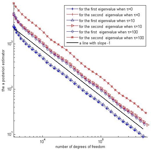
Figure 5: $\tau=0,10,100$, a posteriori error curve of the 1st and the 2nd eigenvalue on the L-shaped domain

where $\Omega\subset R^{2}$ and $\tau$ is the tension coefficient. When $\tau=0$, (5.1)-(5.2) is the vibration problem of a clamped plate without tension.
The weak form of (5.1)-(5.2) and the Morley element approximation is (2.3) and (2.4), respectively, with $n=2$, $a_{ij}=1$, $b_{ij}=\tau$, $\beta=0$ and $\rho=1$.
Weinstein and Chien [37] once obtained lower bounds of eigenvalues for this problem using relaxed boundary conditions in 1943. In section 3 and 4, we analyze the asymptotic lower bounds property and a posteriori error of the Morley element eigenvalues for this problem. Here we provide the numerical results. We compute the first two eigenvalues $\lambda_{j}$, $j=1,2$.
We show the subdivision way for generating initial triangulation for the given unit square and L-shaped domain in Fig. 1.
We use the Morley element on uniform triangle meshes and the conforming Bogner-Fox-Schmit rectangle element (BFS element) on a uniform rectangle meshes to compute, respectively. The numerical results $\lambda_{j,h}^{M}$ and $\lambda_{j,h}^{BFS}$ (j=1,2) are listed in Tables 1-6.
When $\Omega=(0,1)\times(0,\frac{1}{2})\cup(0,\frac{1}{2})\times(\frac{1}{2},1)$ is an L-shaped domain, we use Algorithm $1$ with the Morley element to compute $\lambda_{h_{l}}$ on adaptive meshes with the initial mesh diameter $h=\frac{\sqrt{2}}{32}$. We take $\theta=0.25$ and our program is compiled using the package of Chen [13]. The numerical results $\lambda_{j,h_{l}}^{M}$ (j=1,2) are shown in Tables 7-9.
In Tables 7-9, we use Ndof to denote the number of degrees of freedom.
In Tables 1-6, the discrete eigenvalues $\lambda_{j,h}^{BFS}$ are computed as upper bound.
When $\tau=0$, in Tables 1, 4 and 7, we see that the discrete eigenvalues $\lambda_{j,h}^{M}$ monotonically increase stably, and the Morley elements has already given the lower bounds of eigenvalues, which coincide with Theorem 3.2.
When $\tau>0$, the eigenvalues of this problem are very large. In Tables 5, 6, 8 and 9, we see that the discrete eigenvalues $\lambda_{j,h}^{M}$ monotonically increase stably, and the Morley elements has already given the lower bounds of eigenvalues, which coincide with Theorem 3.1. And the numerical results in Tables 2 and 3 coincide with Theorem 3.3.
When $\Omega$ is an L-shaped domain, we depict the adaptive meshes at the $l$th iteration in Figs.2-4, and the a posteriori error indicator curve in Fig.5.
Comparing the results in Tables 4-6 and 7-9, we see that the approximations on adaptive meshes are more precise than those on uniform meshes.
From Fig.5 it can be seen that the a posteriori error indicator curves are nearly parallel to a line with slope $-1$, which shows that the adaptive algorithm based on the a posteriori error estimators (4)-(4.7) and (4)-(4.12) achieves about the convergence rate of $\mathcal{O}(\frac{1}{Ndof})$ and is successful.

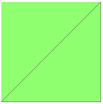
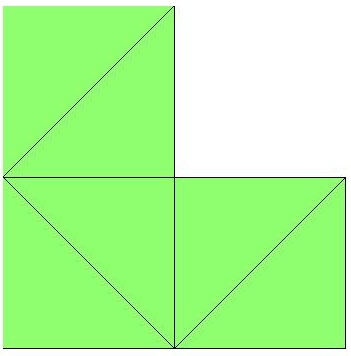
Figure 1: Initial meshs

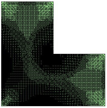
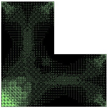
Figure 2: $\tau=0$, adaptive meshes of the 27th iteration for the 1st(left) eigenvalue, and adaptive meshes of the 24th iteration for the 2nd(right) eigenvalue, on the L-shaped domain.

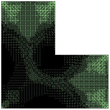
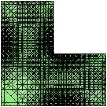
Figure 3: $\tau=10$, adaptive meshes of the 27th iteration for the 1st(left) eigenvalue, and adaptive meshes of the 24th iteration for the 2nd(right) eigenvalue, on the L-shaped domain.

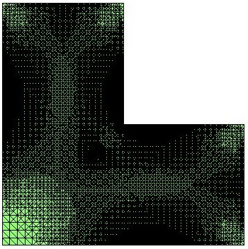
Figure 4: $\tau=100$, adaptive meshes of the 26th iteration for the 1st(left) eigenvalue, and adaptive meshes of the 24th iteration for the 2nd(right) eigenvalue, on the L-shaped domain.

Table 1: $\tau=0$, the 1st and the 2nd eigenvalue on the unit square h Ndof $\lambda_{1,h}^{M}$ $\lambda_{2,h}^{M}$ Ndof $\lambda_{1,h}^{BSF}$ $\lambda_{2,h}^{BSF}$ $\frac{\sqrt{2}}{4}$ 49 691.358 2068.884 36 1300.126 5480.858 $\frac{\sqrt{2}}{8}$ 225 1049.963 3777.006 196 1295.340 5393.253 $\frac{\sqrt{2}}{16}$ 961 1221.316 4850.316 900 1294.963 5387.100 $\frac{\sqrt{2}}{32}$ 3969 1275.511 5239.489 3844 1294.936 5386.685 $\frac{\sqrt{2}}{64}$ 16129 1290.009 5348.921 15876 1294.934 5386.658 $\frac{\sqrt{2}}{128}$ 65025 1293.698 5377.161 64516 1294.934 5386.657 $\frac{\sqrt{2}}{256}$ 261121 1294.625 5384.279 —- —- —-

Table 2: $\tau=10$, the 1st and the 2nd eigenvalue on the unit square h Ndof $\lambda_{1,h}^{M}$ $\lambda_{2,h}^{M}$ Ndof $\lambda_{1,h}^{BSF}$ $\lambda_{2,h}^{BSF}$ $\frac{\sqrt{2}}{4}$ 49 817.866 2340.295 36 1540.868 6059.160 $\frac{\sqrt{2}}{8}$ 225 1232.645 4166.902 196 1534.567 5964.155 $\frac{\sqrt{2}}{16}$ 961 1441.896 5352.314 900 1534.071 5957.503 $\frac{\sqrt{2}}{32}$ 3969 1509.595 5790.254 3844 1534.036 5957.053 $\frac{\sqrt{2}}{64}$ 16129 1527.828 5914.201 15876 1534.033 5957.024 $\frac{\sqrt{2}}{128}$ 65025 1532.476 5946.243 64516 1534.033 5957.022 $\frac{\sqrt{2}}{256}$ 261121 1533.643 5954.323 —- —- —-

Table 3: $\tau=100$, the 1st and the 2nd eigenvalue on the unit square h Ndof $\lambda_{1,h}^{M}$ $\lambda_{2,h}^{M}$ Ndof $\lambda_{1,h}^{BSF}$ $\lambda_{2,h}^{BSF}$ $\frac{\sqrt{2}}{4}$ 49 1842.476 4567.218 36 3660.464 11228.383 $\frac{\sqrt{2}}{8}$ 225 2684.564 7340.279 196 3624.418 11030.745 $\frac{\sqrt{2}}{16}$ 961 3290.809 9629.657 900 3620.928 11014.525 $\frac{\sqrt{2}}{32}$ 3969 3528.551 10614.330 3844 3620.671 11013.347 $\frac{\sqrt{2}}{64}$ 16129 3596.929 10909.494 15876 3620.654 11013.269 $\frac{\sqrt{2}}{128}$ 65025 3614.676 10987.054 64516 3620.653 11013.264 $\frac{\sqrt{2}}{256}$ 261121 3619.156 11006.694 —- —- —-

Table 4: $\tau=0$, the 1st and the 2nd eigenvalue on the L-shaped domain h Ndof $\lambda_{1,h}^{M}$ $\lambda_{2,h}^{M}$ Ndof $\lambda_{1,h}^{BSF}$ $\lambda_{2,h}^{BSF}$ $\frac{\sqrt{2}}{4}$ 33 2026.507 3077.627 20 7571.752 11513.975 $\frac{\sqrt{2}}{8}$ 161 3897.606 6579.447 132 6999.898 11107.297 $\frac{\sqrt{2}}{16}$ 705 5443.844 9332.592 644 6835.442 11062.761 $\frac{\sqrt{2}}{32}$ 2945 6223.547 10541.203 2820 6765.112 11056.385 $\frac{\sqrt{2}}{64}$ 12033 6523.545 10916.025 11780 6732.515 11055.009 $\frac{\sqrt{2}}{128}$ 48641 6632.571 11018.170 48132 6717.205 11054.646 $\frac{\sqrt{2}}{256}$ 195585 6673.866 11045.020 —- —- —-

Table 5: $\tau=10$, the 1st and the 2nd eigenvalue on the L-shaped domain h Ndof $\lambda_{1,h}^{M}$ $\lambda_{2,h}^{M}$ Ndof $\lambda_{1,h}^{BSF}$ $\lambda_{2,h}^{BSF}$ $\frac{\sqrt{2}}{4}$ 33 2248.988 3401.184 20 8095.501 12267.987 $\frac{\sqrt{2}}{8}$ 161 4197.762 7026.946 132 7493.573 11830.283 $\frac{\sqrt{2}}{16}$ 705 5844.849 9933.029 644 7324.642 11784.194 $\frac{\sqrt{2}}{32}$ 2945 6680.697 11225.122 2820 7252.764 11777.697 $\frac{\sqrt{2}}{64}$ 12033 7000.825 11627.366 11780 7219.475 11776.312 $\frac{\sqrt{2}}{128}$ 48641 7116.044 11736.937 48132 7203.839 11775.948 $\frac{\sqrt{2}}{256}$ 195585 7159.231 11765.684 —- —- —-

Table 6: $\tau=100$, the 1st and the 2nd eigenvalue on the L-shaped domain
h Ndof $\lambda_{1,h}^{M}$ $\lambda_{2,h}^{M}$ Ndof $\lambda_{1,h}^{BSF}$ $\lambda_{2,h}^{BSF}$ $\frac{\sqrt{2}}{4}$ 33 4138.743 6220.391 20 12775.204 19033.258 $\frac{\sqrt{2}}{8}$ 161 6676.425 10808.767 132 11854.535 18270.540 $\frac{\sqrt{2}}{16}$ 705 9245.708 15103.285 644 11635.005 18198.392 $\frac{\sqrt{2}}{32}$ 2945 10655.575 17239.122 2820 11548.155 18189.699 $\frac{\sqrt{2}}{64}$ 12033 11189.250 17931.933 11780 11508.527 18188.136 $\frac{\sqrt{2}}{128}$ 48641 11370.095 18121.348 48132 11489.938 18187.754 $\frac{\sqrt{2}}{256}$ 195585 11432.958 18170.592 —- —- —-

Table 7: $\tau=0,\theta=0.25$, the 1st and the 2nd eigenvalue on the L-shaped domain
$l$ Ndof $\lambda_{1,h_{l}}^{M}$ $Ndof$ $\lambda_{2,h_{l}}^{M}$ $l$ $Ndof$ $\lambda_{1,h_{l}}^{M}$ $Ndof$ $\lambda_{2,h_{l}}^{M}$ 1 3201 6218.84 3201 10531.78 20 30033 6688.32 47187 11038.48 2 3249 6345.81 3449 10661.95 21 35293 6690.89 54673 11041.15 3 3403 6416.21 3801 10747.72 22 41310 6693.17 64375 11043.71 4 3531 6456.17 4325 10828.75 23 48473 6695.17 75049 11045.12 5 3829 6512.11 4950 10859.13 24 56871 6696.34 87881 11046.71 6 4173 6536.95 5697 10847.20 25 66047 6697.07 103923 11047.31 7 4643 6578.75 6543 10888.37 26 77216 6697.76 122683 11048.84 8 5131 6584.41 7641 10923.11 27 90500 6698.80 142365 11049.90 9 5793 6605.91 8905 10952.44 28 107015 6699.46 163283 11050.78 10 6569 6623.88 10304 10966.49 29 126197 6700.25 187863 11051.26 11 7623 6637.30 11917 10981.19 30 148263 6700.83 217569 11051.78 12 8803 6649.11 13827 10987.69 31 174145 6701.28 255497 11052.19 13 10201 6658.97 16175 10999.58 32 204237 6701.68 298477 11052.51 14 11753 6661.76 18701 11008.80 33 240145 6701.95 348699 11052.76 15 13621 6667.77 21889 11016.67 34 278865 6702.09 412401 11053.01 16 15833 6674.39 25995 11022.76 35 326744 6702.30 487223 11053.31 17 18437 6679.04 30840 11028.20 36 383793 6702.48 564663 11053.58 18 21655 6683.12 35673 11031.47 37 454113 6702.68 —– —– 19 25453 6685.75 40981 11034.73 38 533383 6702.84 —– —–

Table 8: $\tau=10,\theta=0.25$, the 1st and the 2nd eigenvalue on the L-shaped domain
$l$ Ndof $\lambda_{1,h_{l}}^{M}$ $Ndof$ $\lambda_{2,h_{l}}^{M}$ $l$ $Ndof$ $\lambda_{1,h_{l}}^{M}$ $Ndof$ $\lambda_{2,h_{l}}^{M}$ 1 3201 6675.63 3201 11215.23 20 30733 7173.63 46779 11757.96 2 3257 6809.63 3453 11356.72 21 36195 7176.68 54329 11761.11 3 3423 6891.61 3817 11451.54 22 42307 7179.14 63757 11764.06 4 3575 6934.33 4361 11532.55 23 49763 7181.08 74337 11765.37 5 3897 6994.22 4985 11559.63 24 58131 7182.18 86857 11766.90 6 4237 7013.90 5719 11551.52 25 67479 7182.84 102755 11767.89 7 4735 7052.88 6569 11598.94 26 79069 7183.86 121155 11769.32 8 5231 7067.93 7635 11630.88 27 92839 7184.81 140651 11770.75 9 5919 7088.50 8845 11665.70 28 110135 7185.68 161305 11771.63 10 6722 7104.83 10249 11678.69 29 129399 7186.42 185395 11772.28 11 7755 7118.38 11829 11694.74 30 152321 7187.02 214803 11772.77 12 9005 7132.88 13735 11701.14 31 178795 7187.51 251607 11773.13 13 10417 7141.33 16063 11715.79 32 209879 7187.95 293607 11773.53 14 11957 7145.09 18580 11725.40 33 245095 7188.13 342775 11773.81 15 13906 7152.91 21749 11734.66 34 285181 7188.38 404877 11774.09 16 16120 7158.40 25806 11740.72 35 334009 7188.54 478907 11774.47 17 18869 7163.39 30511 11746.14 36 392889 7188.76 556009 11774.73 18 22219 7168.25 35367 11749.89 37 464649 7188.96 638003 11774.89 19 26145 7170.98 40623 11754.05 38 545321 7189.13 —– —–

Table 9: $\tau=100,\theta=0.25$,the 1st and the 2nd eigenvalue on the L-shaped domain
$l$ Ndof $~{}~{}~{}\lambda_{1,h_{l}}^{M}$ $Ndof$ $~{}~{}~{}\lambda_{2,h_{l}}^{M}$ $l$ $Ndof$ $~{}~{}~{}\lambda_{1,h_{l}}^{M}$ $Ndof$ $~{}~{}~{}\lambda_{2,h_{l}}^{M}$ 1 3201 10647.46 3201 17225.37 20 35207 11445.82 46449 18153.22 2 3297 10862.62 3461 17471.42 21 41155 11451.13 54005 18159.18 3 3491 10982.42 3873 17627.06 22 47783 11454.61 62889 18162.96 4 3739 11066.38 4452 17718.21 23 55501 11457.27 72625 18165.83 5 4165 11139.87 5095 17736.72 24 64329 11458.63 84435 18168.31 6 4613 11203.13 5807 17810.09 25 74704 11460.67 99655 18171.30 7 5135 11230.75 6651 17873.26 26 87138 11462.50 116585 18174.04 8 5782 11271.90 7711 17935.23 27 102486 11464.16 135147 18176.30 9 6661 11305.70 8987 17976.08 28 120434 11465.59 155559 18178.18 10 7673 11331.41 10500 18004.69 29 141483 11466.88 178829 18179.29 11 8911 11355.96 12157 18024.75 30 165055 11467.85 206719 18180.98 12 10391 11374.06 14036 18057.91 31 191875 11469.01 240853 18181.68 13 12041 11386.79 16173 18079.99 32 222691 11469.55 278885 18182.69 14 13923 11401.31 18775 18096.78 33 257621 11469.99 323925 18183.08 15 16129 11412.36 21855 18107.55 34 298901 11470.38 380575 18183.78 16 18701 11420.57 25857 18116.00 35 348221 11470.77 446081 18184.40 17 21847 11428.60 30199 18126.82 36 408785 11471.15 517651 18184.90 18 25721 11434.06 34921 18136.66 37 480267 11471.48 596345 18185.36 19 30135 11438.79 40253 18146.53 38 563307 11471.86 —– —–

6 Concluding remarks

In this paper, for fourth-order elliptic eigenvalue problems with the clamped boundary condition in any dimension, including the vibrations of a clamped plate under tension, we discuss the lower bound property of the Morley element eigenvalues. We prove on regular meshes, including adaptive local refined meshes, that in the asymptotic sense the Morley element eigenvalues approximate the exact ones from below, which is a development of the work in [19, 22, 40]. Our analysis is an application of the identity (3.1), in which higher order contributions are identified.
Our analysis and results about the lower bound property of the Morley element eigenvalues can be applied to general $2m$-th order elliptic eigenvalue problems (see (6.5) in [19]).

Acknowledgements.  This work was supported by the National Natural Science Foundation of China (Grant Nos.11161012,11201093).

References

- [1] M. Ainsworth, J.T. Oden, A posteriori error estimates in the finite element analysis. New York: Wiley-Inter science, 2011.
- [2] M. Ainsworth, Robust a posteriori error estimation for nonconforming finite element approximation, SIAM J. Numer. Anal., 42 (2005): 2320-2341.
- [3] M.G. Armentano, R.G. Duran, Asymptotic lower bounds for eigenvalues by nonconforming finit element methods, Electron Trans Numer. Anal., 17 (2004), pp. 92-101.
- [4] I. Babuka, J. Osborn, Eigenvalue Problems, Handbook of Numerical Analysis. vol.2, North-Holand: Elsevier Science Publishers B.V., 1991.
- [5] I. Babuka, R.B. Kellog, Pitkaranta J. Direct and inverse error estimates for finite elements with mesh refinement, Numer. Math., 33 (1979), pp. 447-471.
- [6] I. Babuka, A. Miller, A feedback finite element method with a posteriori error estimation: Part I. The finite element method and some basic properties of the a posteriori error estimator, Comput. Methods Appl. Mech. Engrg., 61 (1987), pp. 1-40.
- [7] Veiga L. Beiro da, J. Niiranen, R. Stenberg, A posteriori error estimates for the Morley plate bending element, Numer. Math., 106 ( 2007), pp. 165-179.
- [8] R. Becker, S. Mao, Z. Shi, A Convergent nonconforming adaptive finite element method with quasi-optimal complexity, SIAM J. Numer. Anal., 47(6) (2010), pp. 4639-4659.
- [9] H. Blum, R. Rannacher, On the boundary value problem of the biharmonic operator on domains with angular corners, Math. Method. Appl. Sci., 2 (1980), pp. 556-581.
- [10] S.C. Brenner, L.R. Scott, The Mathematical Theory of Finite Element Methods. 2nd ed., Springer-Verlag, New york, 2002.
- [11] C. Carstensen, D. Gallistl, Guaranteed lower eigenvalue bounds for the biharmonic equation. Numer. Math., 1 (2014), pp. 33-51.
- [12] C. Carstensen, J. Hu, A. Orlando, Framework for the a posteriori error analysis of nonconforming finite elements. SIAM J. Numer. Anal., 45(1) (2007), pp. 68-82.
- [13] L. Chen, iFEM: an innovative finite element methods package in MATLAB, Technical Report, University of California at Irvine, 2009.
- [14] P.G. Ciarlet, Basic error estimates for elliptic proplems. Handbook of Numerical Analysis, vol.2, North-Holand: Elsevier Science Publishers B.V., 1991.
- [15] X. Dai, J. Xu, A. Zhou, Convergence and optimal complexity of adaptive finite element eigenvalue computations. Numer. Math., 110 (2008), pp. 313-355.
- [16] R.G. Durn, C. Padra, R. Rodrguez, A posteriori error estimates for the finite element approximation of eigenvalue problems, Math. Mod. Meth. Appl. Sci., 13 (2003), pp.1219-1229.
- [17] D. Gallistl, Morley Finite Element Method for the Eigenvalues of the Biharmonic Operator, arXiv:1406.2876 [math.NA], 2014
- [18] J. Gedicke and C. Carstensen, A posteriori error estimators for convection-diffusion eigenvalue problems, Comput. Methods Appl. Mech. Engrg., 268(2014), pp.160-177.
- [19] J. Hu, Y. Huang, Q. Lin, Lower bounds for eigenvalues of elliptic operators: By Nonconforming finite element methods, J. Sci. Comput., 61(2014), pp.196-221
- [20] J. Hu, Z. Shi, A new a posteriori error estimate for the Morley element, Numer. Math., 112(1)(2009), pp. 25-40.
- [21] P. Lascaux, P. Lesaint, Some nonconforming finite elements for the plate bending problem, Rev. Francaise Automat. Informat. Recherche Operationnelle Ser Rouge Anal Numer, R-1(1975), pp. 9-53.
- [22] Q. Lin, H. Xie, Recent results on lower bounds of eigenvalue problems by nonconforming finite element methods. Inverse Problems and Imaging, 7(3) (2013), pp. 795-811.
- [23] Q. Lin, H. Xie, J. Xu, Lower bounds of the discretization for piecewise polynomials, Math. Comp., 83(285) (2014), pp. 1-13.
- [24] F. Luo, Q. Lin, H. Xie, Computing the lower and upper bounds of Laplace eigenvalue problem: by combining conforming and nonconforming finite element methods. Sci. China Math., 55 (2012), pp. 1069-1082.
- [25] S. Mao, S. Nicaise, Z. Shi, Error estimates of Morley triangular element satisfying the maximal angle condition. Int. J. Numer. Anal. Model., 7 (2010), pp. 639-655.
- [26] P. Morin, R.H. Nochetto, K. Siebert, Convergence of adaptive finite element methods. SIAM Rev, 44 (2002), pp. 631-658.
- [27] L.S.D. Morley, The triangular equilibrium element in the solution of plate bending problems, Aero Quart 19 (1968), pp. 149-169.
- [28] J. T. Oden, J. N. Reddy, An Introduction to the Mathematical Theory of Finite Elements, Courier Dover Publications, New York, 2012.
- [29] R. Rannacher, Nonconforming finite element methods for eigenvalue problems in linear plate theory, Numer. Math., 33 (1979), pp. 23-42.
- [30] Q. Shen A posteriori error estimates of the Morley element for the fourth order elliptic eigenvalue problem, Numer. Algor., 68 (2015), pp. 455-466
- [31] Z. Shi, On the error estimates of Morley element. Chinese J. Numer. Math. & Appl., 12 (1990), pp. 102-108.
- [32] Z. Shi, M. Wang, Finite Element Methods. Beijing, Scientific Publishers, 2013.
- [33] G. Strang, G.J. Fix, An alalysis of the finite element method. Prentice-Hall, 1973.
- [34] R. Verfrth, A review of a posteriori error estimates and adaptive mesh-refinement techniques. New York: Wiley-Teubner, 1996.
- [35] M. Wang, J. Xu, The Morley element for fourth order elliptic equations in any dimensions. Numer. Math., 103(2006), pp. 155-169.
- [36] M. Wang, J. Xu, Minimal finite-element spaces for 2m-th order partial differential equations in . Math Camp, 82(2013), pp. 25-43.
- [37] A. Weinstein, W.Z. Chien, On the vibrations of a clamped plate under tension, Quarterly of Applied Mathematics, 1(1) (1943), pp. 61-68.
- [38] O. Widlund, On best error bounds for approximation by piecewise polynomial functions. Numer. Math., 27 (1977), pp. 327-338.
- [39] Y. Yang, Z. Zhang, F. Lin, Eigenvalue approximation from below using nonforming finite elements. Sci. China Math., 53(1) (2010), pp. 137-150.
- [40] Y. Yang, Q. Lin, H. Bi, Q. Li, Lower eigenvalues approximation by Morley elements. Adv. Comput. Math., 36(3) (2012), pp. 443-450.
- [41] Y. Yang, J. Han, H. Bi, Y. Yu, The lower/upper bound property of the nonoconforming Crouzeix-Raviart element eigenvalues on adaptive meshes. J. Sci. Comput., 62(1) (2015), pp. 284-299.
- [42] Y. Yang, A posteriori error analysis of conforming/nonconforming finite elements (in Chinese), Sci. Sin. Math., 40(9) (2010), pp. 843-862.
- [43] Z. Zhang, Y. Yang, Z. Chen, Eigenvalue approximation from below by Wilson’s element. Chinese J. Numer. Math. & Appl., 29(4) (2007), pp. 81-84.