Identification of Source of Rumors in Social Networks with Incomplete Information

Abstract

Rumor source identification in large social networks has received significant attention lately. Most recent works deal with the scale of the problem by observing a subset of the nodes in the network, called sensors, to estimate the source. This paper addresses the problem of locating the source of a rumor in large social networks where some of these sensor nodes have failed. We estimate the missing information about the sensors using doubly non-negative (DN) matrix completion and compressed sensing techniques. This is then used to identify the actual source by using a maximum likelihood estimator we developed earlier, on a large data set from Sina Weibo. Results indicate that the estimation techniques result in almost as good a performance of the ML estimator as for the network for which complete information is available. To the best of our knowledge, this is the first research work on source identification with incomplete information in social networks.

1 Introduction

On April $2013$, hackers took control of the Twitter account @AP and sent a fake tweet about explosions in the White House. U.S. financial markets were spooked by this tweet; the index value of S&P $500$ dropped $14$ points, wiping out $\$136.5$ billion in a matter of seconds before the financial markets recovered[1]. At a time when cybersecurity has become a major national issue, the ease of rumor spread through social networks has exacerbated concerns. More specifically, studies show that rumors spread much faster in social networks than other type of networks, even faster than networks with complete graph topology[2]. Therefore, it is of great interest to pinpoint the source of the rumor in time by leveraging the social network topology and observing the state of nodes. The practical applications include rapid damage control and understanding the role of network structure in rumor dissemination, thereby facilitating the design of sophisticated policies to prevent further viral spreading of misinformation through social networks in the future.

The various approaches in locating the source of a rumor may be classified based on whether they rely on observing all the nodes in the social network [3, 4, 5, 6, 7, 8, 9] or a fraction of nodes in the social network[10, 11]. It is impractical to observe all the nodes in the social network due to the large amount of the computational complexity that is involved. One means to deal with the complexity issues is by selecting a subset of nodes (also called sensors) [10, 11]. In [10], a maximum likelihood (ML) estimator was proposed using measurements by the sensors. It was shown that an average source localization error of less than $4$ hops can be achieved by observing $20\%$ of the nodes in network. In [11] we proposed a two-stage source localization algorithm that required $3\%$ less sensor nodes to provide measurements on the time of arrival of information, and yet provided results with the same accuracy as previous studies.

In most practical scenarios, it is not possible to observe the status of all nodes in a large-scale social network. Therefore, the source of rumor must be located based on the measurements collected by a subset of nodes (called sensors) in the social network. The sensors record the arrival times of the rumor to estimate the most likely source. However, in most practical scenarios, we may not have complete information on the time at which the sensors receive the rumor. This could happen because most social networks such as Twitter do not provide public access to their full stream of tweets and many Facebook users keep their activity and profiles, private. Overall, the rapid growth of the social networks themselves, and the increasing volume of their generated data, will likely augment the problem of missing data in the study of rumor diffusion. This paper presents a technique to locate the source of a rumor for large social networks where the information on the time at which the sensors receive the rumor is incomplete.

Using incomplete information to estimate the source of rumors is achieved by recovering the missing information. Such data recovery was addressed in the context of computer networks [12] and sensor networks [13]. In the context of social networks, recovering the missing information is essentially a matrix completion problem. There are several approaches to matrix completion [14, 15, 16, 17, 18]. We deploy compressed sensing [14, 15] and doubly non-negative (DN) matrix completion [16, 17, 18] to recover the missing information on the time epochs at which certain sensors receive the information. We also present a renewal theory-based argument to improve the DN completion based estimation. We use the estimated values to identify the source of rumors using a maximum likelihood (ML) estimator we developed in [11]. Results indicate that these estimation methods provides us with almost as good a performance of source identification as that when complete information is available.

The rest of the paper is organized as follows. In Section 2, the rumor diffusion model and the source estimator are discussed. Section 3 presents different approaches to recover missing values at the sensors using compressed sensing, DN matrix completion, and renewal theory-based model. Experimental results are provided in Section  4 and conclusions in Section 5.

2 Source Identification

The source identification mechanism we designed in [11] is as follows. A social network can be modeled as a graph, $G(V,E)$, where a vertex, $v\in V$ represents a user in the network and two vertices, $u$, $v\in V$ share an edge if the corresponding users share a friendship or any similar relation. Whenever a user tweets or posts a message (or a rumor), the people following the user or the friends of the user may re-tweet or re-post the rumor. Let $t_{mn}$ be the delay between the epochs at which nodes, $m$ and $n$ get “infected” by a rumor. Then $t_{mn}\sim\mathcal{N}(\mu_{mn},\sigma_{mn}^{2})$ [10]. The parameters, $\mu_{mn}$ and $\sigma_{mn}^{2}$ depend on the path between the nodes, $m$ and $n$. A source, $s^{*}$, starts a rumor and spreads it on a social network. The information diffuses through the network and reaches nodes, $v\in V$ along the shortest path from $s$ to $v$. The goal is to determine $s^{*}$ given the time epochs at which nodes, $v\in S\subset V$ (the set of sensor nodes) receive the information.

The source localization algorithm consists of two stages. In the first stage, the cluster that most likely contains the source of the rumor is identified and then, in the second stage, we search within this cluster and identify the source of the rumor. A new graph $G^{\rm gate}=(V^{\rm gate},E^{\rm gate})$, where $V^{\rm gate}$ is the gateway nodes (nodes connecting clusters using between-cluster ties), $E^{\rm gate}$ is incident on the vertices in $V^{\rm gate}$. Let $S=\{l_{1},l_{2},...,l_{k_{1}}\}$ be a set of $k_{1}$ nodes, selected from $V_{\rm gate}$, to observe the time arrival of the rumor. Since the time that the source starts to spread information, ${t^{*}}$, is typically unknown, inter-arrival times, ${\Delta{t_{i}}}\buildrel\Delta\over{=}({t_{i}}+{t^{*}})-({t_{1}}+{t^{*}})={t_{i}}-{t_{1}}$, can be used for estimation, where $t_{i}$ is the time at which the rumor is received at the $i^{\mathrm{th}}$ sensor in $G^{\rm gate}$. The inter-arrival time observation vector is then defined as ${\mathbf{\Delta{t^{stage1}}}}=[\Delta{t_{2}},\Delta{t_{3}},...,\Delta{t_{k-1}}]^{T}$ . Since, all the nodes are equally likely to be the source of a rumor, the maximum likelihood (ML) estimator is the optimal estimator for the source of the rumor, described as

$$\begin{split}\hat{v}^{(1)}&=\\ &\mathop{\arg{\rm{max}}}\limits_{v\in{V^{gate}}}~{}\frac{1}{{{(2\pi)^{\frac{{{k_{1}}-1}}{2}}}\det{{({\mbox{\boldmath$\Lambda$}_{v}})}^{1/2}}}}\times\\ &\exp(-\frac{1}{2}{(\mathbf{\Delta{t^{stage1}}}-{\mbox{\boldmath$\mu$}_{v}})}{({\mbox{\boldmath$\Lambda$}_{v}})^{-1}}(\mathbf{\Delta{t^{stage1}}}-{\mbox{\boldmath$\mu$}_{v}})^{T}),\end{split}$$ (1)

where ${\mbox{\boldmath$\mu$}_{v}}(r)$ is the mean value of difference in arrival times between the first and the $(r+1)^{\mathrm{th}}$ sensors and $\mbox{\boldmath$\Lambda$}_{v}(a,b)$ is the cross-correlation matrix of difference in arrival times between the $a^{\mathrm{th}}$ and the $b^{\mathrm{th}}$ sensors.

In the second stage, the search space will be limited to the nodes inside the cluster that is associated with $\hat{v}^{(1)}$. Let $G^{\rm cluster}=(V^{\rm cluster},E^{\rm cluster},\mathbf{w}^{\rm cluster})$ be the graph of the nodes inside the most likely candidate cluster. $k_{2}$ sensors are employed at this stage to collect information about the rumor. The corresponding optimal ML estimator is given by

$$\begin{split}{\hat{v}^{(2)}}=&\\ &\mathop{\arg{\rm{max}}}\limits_{v\in{V^{cluster}}}~{}\frac{1}{{\det{{({\mbox{\boldmath$\Lambda$}_{v}})}^{1/2}}}}\\ &\exp(-\frac{1}{2}{(\mathbf{\Delta{t^{stage2}}}-{\mbox{\boldmath$\mu$}_{v}})}{({\mbox{\boldmath$\Lambda$}_{v}})^{-1}}(\mathbf{\Delta{t^{stage2}}}-{\mbox{\boldmath$\mu$}_{v}})^{T})\end{split}$$ (2)

where $\mathbf{\Delta{t^{stage2}}}$ is the observation vector in the second stage and ${\hat{v}^{(2)}}$ is the estimated source of the rumor. Detailed information about the two-stage algorithm can be found in [11]. It is observed that the ML source estimator requires full information about the vectors, $\mbox{\boldmath{$\Delta$}}\mathbf{t}^{\rm stage1}$ and $\mbox{\boldmath{$\Delta$}}\mathbf{t}^{\rm stage2.}$ In most practical scenarios, we may not have the entire information on the time epochs at which different sensors receive the information. This could be because most social networks such as Twitter do not provide public access to their full stream of tweets and most Facebook users keep their activity and profiles private. In the following section, we present estimation mechanisms that enable source identification when incomplete information about $\mbox{\boldmath{$\Delta$}}\mathbf{t}^{\rm stage1}$ and $\mbox{\boldmath{$\Delta$}}\mathbf{t}^{\rm stage2.}$ is available.

3 Source Identification with Partial Information

We present three different approaches to recover the missing information, which, in turn, will be used in the analysis to identify the source, as detailed in Section 2. First, we present a compressed sensing based approach (Section 3.1) that is effective in recovering sporadically missing information. Then we present an approach using doubly non-negative (DN) matrix completion to recover information missing in bursts, in Section 3.2. Then, in Section 3.3, we improve the DN completion mechanism by using a renewal theory-based analysis.

3.1 Compressed Sensing

Consider a observation vector $\mathbf{\Delta t}=[\Delta{t_{1}},\Delta{t_{2}},...,\Delta{t_{K}}]^{T}$, where $\Delta{t_{i}}$ corresponds to difference in arrival times between the $i^{th}$ sensor and the reference sensor. Let $y\in\mathbb{R}^{L}$ be the vector of available entries in $\mathbf{\Delta t}$ where $L\leq K$. Hence,

$$\mathbf{y}=\phi\mathbf{\Delta t}$$ (3)

where $\phi$ is an $L\times K$ measurement matrix. In order to recover the original observation vector $\mathbf{\Delta t}$ from $\mathbf{y}$, we assume that there exists an invertible $K\times K$ sparsifying matrix $\psi$ such that

$$\mathbf{\Delta t}=\psi\mathbf{x}$$ (4)

where $\mathbf{x}\in\mathbb{R}^{K}$ is M-sparse with $M\leq L$, i.e., it has only $M$ non-zero entries. Using Eqn.(3) and Eqn.(4) we can write

$$\mathbf{y}=\phi\mathbf{\Delta t}=\phi\psi\mathbf{x}=\theta\mathbf{x}$$ (5)

that is, in general, an ill-posed and ill-conditioned with $\theta=\phi\psi$ of dimensions $L\times K$. Infinitely many solutions are possible unless we impose some additional constraints on $\mathbf{\Delta t}$. Since the rumor spread along the shortest paths in the social network, the observation vector shows some amount of correlation among its elements. The correlation structure of the observation vector makes it possible to acquire sufficiently accurate representations of the observation vector without collecting time arrivals from each sensor node. Therefore, the vector $\mathbf{\Delta t}$ can be approximated by a low-rank vector $\mathbf{x}$. Therefore, the problem becomes

$$\underset{\mathbf{x}}{\text{min}} {\left\|\mathbf{x}\right\|_{{\ell_{1}}}}$$ (6)

s.t. $$\mathbf{y}=\theta\mathbf{x}$$

where ${\left\|\mathbf{x}\right\|_{{\ell_{1}}}}$ is the $\ell_{1}$-norm of $\mathbf{x}$.

Ultimately the estimated time arrival vector $t_{\textrm{est}}$ is

$$\mathbf{\Delta t}_{\textrm{est}}=\psi\mathbf{x}_{\textrm{opt}}$$ (7)

where $\mathbf{x}_{\textrm{opt}}$ is the solution to the problem in Eqn. 6.

3.2 DN completion

There are certain scenarios, where in the information on the time epochs of information arrival at different users corresponding to sensor nodes, may be missing in bursts. This could happen because certain users that act as sensors, remain idle, temporarily. Let $X_{ij}$ denote the time delay between the epochs when information propagated by sensor node $i$ and that when it reaches node $j$. The delay between different nodes can then be written as a matrix, $\mathbf{D}=\left[X_{ij}\right]_{i,j\in\mathbf{S}}$, where $\mathbf{S}$ is the set of all sensor nodes. Note that in $\mathbf{D}$, $X_{ii}=0$, $\forall$ $i$.
When some nodes temporarily get de-activated or unsubscribe as a sensor, then the matrix, $\mathbf{D}$, has certain entries missing. If the set of missing entries occur in bursts, then techniques like matrix completion can be used to determine the missing entries in the matrix, $\mathbf{D}$ [16]. These include inverse $\mathcal{M}-$matrix completion [17], doubly non-begative (DN) completion [18]. In order to perform these matrix completions, it is essential that the matrix, $\mathbf{D}$ represented as a graph the graph forms a block clique [19]. Then $\mathbf{D}$ is symmetric and of the form

$$\mathbf{D}=\left(\begin{array}[]{ccc}\mathbf{A}&\mathbf{c}&\mathbf{X}\\ \mathbf{c}^{T}&e&\mathbf{d}^{T}\\ \mathbf{X}^{T}&\mathbf{d}&\mathbf{B}\end{array}\right),$$ (11)

where $e$ is any constant, $\mathbf{A}$ is a known $m\times m$ sub-matrix, with entries $a_{ij}=X_{ij}$, the time delay between pairs of the first $m$ sensors, $\mathbf{c}$ is an $m\times 1$ vector, $\mathbf{d}^{T}$ is a $1\times n$ vector and $\mathbf{B}$ is another $n\times n$ sub-matrix. An optimal mechanism for DN completion of such a matrix was discussed in [12], which we use here to estimate the missing delays between the times at which different sensor nodes obtain information. According to the analysis in [12],

$$\mathbf{X}=\mathbf{D}_{\alpha}\mathbf{c}\mathbf{d}^{T}\mathbf{D}_{\beta},$$ (12)

where $\mathbf{D}_{\alpha}=$diag$(\alpha_{1},\alpha_{2},\cdots,\alpha_{m})$ and $\mathbf{D}_{\beta}=$diag$(\beta_{1},\beta_{2},\cdots,\beta_{n})$. Based on the values of $E(\mathbf{X})=E\left(\left[X_{ij}\right]_{1\leq i\leq m\atop 1\leq j\leq n}\right)$, the optimal values of $\mbox{\boldmath{$\alpha$}}=\left[\alpha_{i}\right]_{1\leq i\leq m}$ and $\mbox{\boldmath{$\beta$}}=\left[\beta_{j}\right]_{1\leq j\leq n}$, that minimize the mean square error in estimation (i.e., the MMSE estimate [20]), is given by the iterative set of equations [12]

$$\mbox{\boldmath{$\alpha$}}=\frac{E(\mathbf{X})\mbox{\boldmath{$\beta$}}}{||\mbox{\boldmath{$\beta$}}||^{2}}$$ (13)

$$\mbox{\boldmath{$\beta$}}=\frac{E(\mathbf{X}^{T})\mbox{\boldmath{$\alpha$}}}{||\mbox{\boldmath{$\alpha$}}||^{2}}.$$ (14)

It was shown in [12] that the set of iterative equations in Eqns. (13) and (14) converge if the condition number of the co-variance matrix of $\mathbf{X}$ is less than $2$. This can be satisfied by adding sufficiently large values to the diagonal elements of $\mathbf{D}$ (i.e., have $d_{ii}$ as a very large value instead of $0$).

3.3 Renewal Theory-based Model

The rumor dissemination process is depicted in Figure 1 as a function of time. The user corresponding to the $i^{th}$ sensor first receives the information at time, $Z_{ij}^{(1)}=X_{ij}^{(1)}$. Then the $i^{th}$ sensor is idle for a period of time, $S_{2}$ and then relays the information at a time $X_{ij}^{(1)}+S_{2}$. The information is received by the $j^{th}$ sensor at a time, $Z_{ij}^{(2)}=X_{ij}^{(1)}+S_{2}+X_{ij}^{(2)}$. In general, the $i^{th}$ sensor receives the information for the $m^{th}$ time at an epoch $Z_{ij}^{(m)}$, stays idle for a time interval of length, $S_{m+1}$ and transmits the information at an epoch $Z_{ij}^{(m)}+S_{m+1}$, which is received by the $j^{th}$ sensor for the $(m+1)^{th}$ time at an epoch, $Z_{ij}^{(m)}+S_{m+1}+Z_{ij}^{(m+1)}$.This can be considered as a renewal process with vacations [21].

Remark 3.1

Note that the renewal process will not be contiguous in time, as represented in Figure 1. This is because, between the epoch when sensor $i$ receives the information for the $(m-1)^{th}$ time and the $m^{th}$ time, there is a time delay. However, that delay will not affect the renewal theory-based analysis since we are interested in determining the average time delay between the time epochs when the $i^{th}$ and $j^{th}$ sensors receive the information. In other words, the blank period between the successive time instants the $i^{th}$ sensor receives the information does not affect the renewal process.

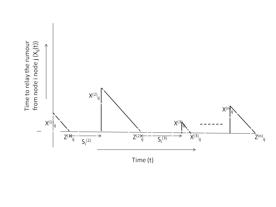
Figure 1: Timing diagram of the process according to which sensor $i$ receives the rumor and disseminates it to sensor $j$. Sensor $i$ is idle or inactive for times, $S_{i}^{(m)}$, $m\geq 2$ and in the $m^{th}$ dissemination attempt, takes a time, $X_{ij}^{(m)}$ to actually reach node $j$ after the information is transmitted.

The time intervals, $X_{ij}^{(1)}$, $X_{ij}^{(2)}$, $\cdots$, $X_{ij}{(n)}$, $\cdots$, are independent where $X_{ij}^{(1)}\sim A_{ij}$, i.e., $\Pr\{X_{ij}^{(1)}\leq x\}=A_{ij}(x)$ and $X_{ij}^{(m)}\sim F_{ij}$, i.e., $\Pr\{X_{ij}^{(m)}\leq x\}=F_{ij}(x)$, $m\geq 2$. Similarly, $S_{k}$, $k\geq 2$ are independent and identically distributed (iid) $S_{k}\sim V(x)$, $\forall$ $k$, i.e., $\Pr\S_{k}\leq x\}=V(x)$, $\forall$ $k$. Let $a(x)=\frac{dA(x)}{dx}$, $f(x)=\frac{dF(x)}{dx}$ and $v(x)=\frac{dV(x)}{dx}$, i.e., the probability density function (pdf) of $X_{ij}^{(1)}$, $X_{ij}^{(m)}$, $m\geq 2$, and $S_{k}$, $k\geq 2$ are $a_{ij}(x)$, $f_{ij}(x)$ and $v(x)$, respectively.

At any time epoch, $t$, let $Y_{ij}(t)$ be defined as the remaining time or residual transmission time of the information from sensor $i$ to the sensor $j$. Let $\mathbf{Y}(t)=\left[Y_{ij}(t)\right]_{i,j\in\mathbf{S}}$; $\mathbf{S}$ is the set of sensors. Then in the analysis for the DN completion described in Section 3.2, specifically, we use $\lim_{t\rightarrow\infty}E[\mathbf{Y}(t)]$, instead of $E(\mathbf{X})$ in Eqns. (13) and (14). The following theorems from renewal theory will be used to characterize $E[\mathbf{Y}(t)]$.

Theorem 3.2

[21] Consider a renewal process where the life time of the $l^{th}$ renewal is $X_{l}$. Let $X_{1}\sim G(x)$, with pdf, $g(x)=\frac{dG(x)}{dx}$ and $X_{2}$, $X_{3}$, $\cdots\sim H(x)$, with pdf, $h(x)=\frac{dF(x)}{dx}$. Let

$$\frac{1}{\mu}\stackrel{{\scriptstyle\triangle}}{{=}}E(X)=\int_{0}^{\infty}[1-H(x)]dx=\int_{0}^{\infty}xh(x)dx.$$ (15)

Then the cumulative distribution function (CDF) of $Y(t)$, $R(x)$ and the pdf of $Y(t)$, $r(x)=\frac{dR(x)}{dt}$, are given by

$$\begin{array}[]{ccc}R(x)&=&\lim_{t\rightarrow\infty}\frac{1}{t}\int_{u=0}^{t}\Pr\{Y(u)\leq x\}du\\ &=&\mu\int_{u=0}^{x}[1-H(u)]du,\end{array}$$ (18)

$$r(x)=\mu[1-H(x)].$$ (19)

Moreover,

$$E[(Y)]=\mu\int_{x=0}^{\infty}x^{2}h(x)dx=\mu E(X_{k}^{2}),k\geq 2,$$ (20)

which, in turn, can be re-written as

$$E[(Y)]=\frac{E(X_{k})}{2}\left(1+C_{X}^{2}\right),$$ (21)

where

$$C_{X}^{2}=\frac{Var(X_{k})}{\left[E(X_{k})\right]^{2}},k\geq 2.$$ (22)

Theorem 3.3

[21] Let $K_{y}(t)\stackrel{{\scriptstyle\triangle}}{{=}}\Pr\{Y(t)\leq y\}$. Then

$$\begin{array}[]{ccc}\lim_{t\rightarrow\infty}K_{y}(t)&=&R(y),\\ \lim_{t\rightarrow\infty}[E(Y(t)]=\frac{E(X_{k})}{2}\left(1+C_{X}^{2}\right),\end{array}$$ (25)

where $C_{X}^{2}$ is given by Eqn. (22).

From Theorems 3.2 and 3.3, The average remaining time for information to reach from sensors to each other, $E(\mathbf{Y})$, which we use in Eqns. (13) and (14) is

$$E\left(Y_{ij}\right)=\frac{E\left(X_{ij}\right)+E\left(S_{i}\right)}{2}\left(1+\frac{Var\left(X_{ij}\right)+Var\left(S_{i}\right)}{\left[E\left(X_{ij}\right)+E\left(S_{i}\right)\right]^{2}}\right).$$ (26)

In Eqn. (26), $E\left(X_{ij}\right)+E\left(S_{i}\right)$ is the value $E(X_{ij})$ used in DN completion in Section 3.2, without applying the renewal theory-based analysis discussed in this subsection. The expression for $E\left(Y_{ij}\right)$ from Eqn. (26) is substituted in Eqns. (13) and (14) to obtain the modified DN completion using the renewal argument. The $\mbox{\boldmath{$\Delta$}}\mathbf{t}$ estimated in Sections 3.1-3.3 are in used in the ML estimator described in Section 2, to identify the source of the rumor.

4 Results and Discussion

We conduct our experiments on the Sina Weibo dataset in [22]. Sina Weibo is the most popular microblogging service in China [23]. This dataset includes a followership network with $58,655,849$ nodes and $265,580,802$ edges, and a total of $370$ million tweets and retweets. The retweeting paths (with their time-stamps) are provided which is suitable in particular for studying real information dissemination networks. We selected $100$ tweets from this dataset which constitute $100$ different real diffusion networks. Table 1 summarizes the details of the dataset. We used the Louvain method [24] to identify the clusters, as the gateway nodes of these clusters are used to construct the gateway graph $G^{\rm gate}$. Since it is assumed that rumors spread along the shortest paths into the social network, we selected nodes with high betweenness centrality as sensors.

Table 1: Details of dataset

	Max	Ave	Min
Number of nodes	$43,545$	$41,978$	$40,445$
Number of edges	$84,451$	$82,790$	$80,923$
Diameter	$13$	$11$	$9$
Average shortest path length	$8.31$	$5.97$	$4.71$
Number of clusters	$223$	$148$	$103$

Figure 2 shows the accuracy of recovering the missing entries in $\mathbf{{\Delta t}}$ (employing compressed sensing) vs the percentage of nodes used as sensors. The accuracy is defined as the mean square error (MSE) between the original and the estimated missing entries. We randomly remove $15\%$ and $30\%$ of the entries sporadically to simulate the missing measurements. As can be seen from this graph, the estimation error is smaller when the missing rate is smaller. It could be due to the fact that the number of remaining entries after $30\%$ missing is less sufficient to precisely estimate the missing entries. However, the error gap between the $15\%$ and the $30\%$ missing rates is very small when the percentage of sensors is less than $0.3\%$.

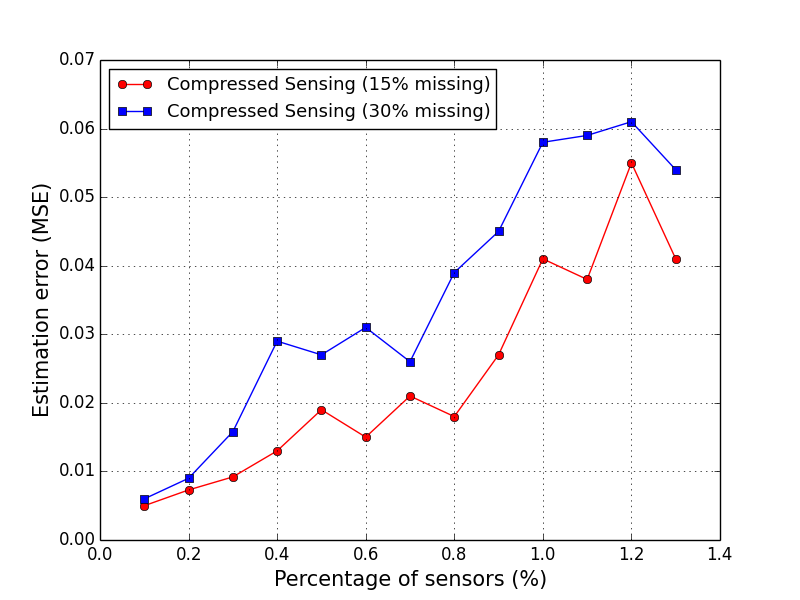
Figure 2: Estimation error for the observation vector $\mathbf{{\Delta t}}$ when $15\%$ and $30\%$ of entries are missing and deploying compressed sensing (described in Section 3.1).

To evaluate the DN completion approach, a sub-matrix of $D$ is removed. The removed sub-matrix is chosen such that the graph representation of the partial matrix forms a block clique. Figure 3 shows the estimation error of the DN completion. The renewal based argument provides less estimation error because it utilizes the first two moments of the dissemination intervals as opposed to the DN matrix completion method which uses only the first moment. It also shows that the accuracy improvement is larger when the missing rate is $15\%$.

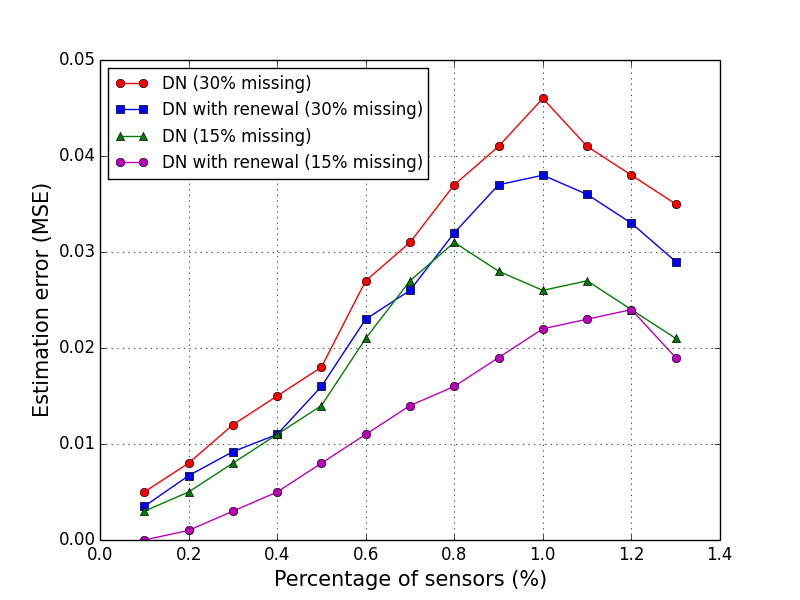
Figure 3: Estimation error for the observation vector $\mathbf{{\Delta t}}$ when the missing rate is $0\%$ (not missing measurements), $15\%$, and $30\%$ and deploying DN matrix completion (Section 3.2) and renewal based argument (Section 3.3). The renewal theory based mechanism results in lower error because it utilizes the first two moments of the missing measurements while the DN completion method uses only the first moment.

Next, we study the accuracy of the source estimation using compressed sensing. The accuracy is measured in average distance between the estimated and the actual sources. Figure 4 shows the source estimation error when the missing rate is $0\%$ (no missing measurements), $15\%$, and $30\%$. It shows that compressed sensing results in almost as good a performance of the ML estimator as for the network for which complete information is available. Figure 5 shows the source estimation error when deploying DN matrix completion and renewal-based argument. We again observe that the renewal based argument provides less estimation error in source localization. Results indicate that the estimation techniques result in almost as good a performance of the ML estimator as for the network for which complete information is available.

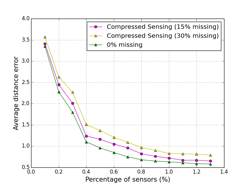
Figure 4: Average distance between the estimated source and the actual source when $15\%$ and $30\%$ of entries in $\mathbf{{\Delta t}}$ are missing and deploying compressed sensing (described in Section 3.1).

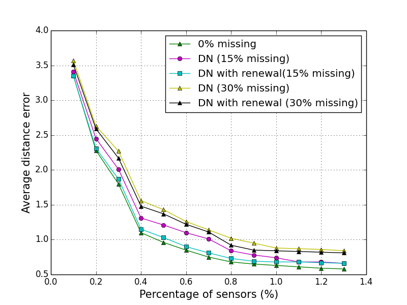
Figure 5: Average distance error between the estimated source and the actual source when $15\%$ and $30\%$ of entries in $\mathbf{{\Delta t}}$ are missing and deploying DN matrix completion (Section 3.2) and renewal-based argument (Section 3.3). The renewal based argument provides less estimation error in source localization.

5 Conclusions

We addressed the problem of locating the source of a rumor in large-scale social networks with incomplete measurements. We presented the compressed sensing method to recover sporadically missing measurements and the doubly non-negative (DN) completion to recover measurements missing in bursts. Furthermore, we presented a renewal theory-based model to boost the performance of the DN matrix completion method. We then used the recovered measurements to estimate the source of the rumor. We observed that the compressed sensing and the DN matrix completion provide less estimation error when the percentage of missing entries is less. It is also shown that the renewal theory-based model increases the accuracy improvement of the DN matrix completion method. Mechanisms to jointly improve the ML estimator as well as the estimation of missing measurements, is under investigation.

References

- [1] G. Strauss, A. Shell, R. Yu, and B. Acohido, “SEC, FBI probe fake tweet that rocked stocks,” Apr. 2013. [Online]. Available: http://www.usatoday.com/story/news/nation/2013/0 4/23/hack-attack-on-associated-press-shows-vulnerable-media/2106985/
- [2] B. Doerr, M. Fouz, and T. Friedrich, “Social networks spread rumors in sublogarithmic time,” in Proceedings of the Forty-third Annual ACM Symposium on Theory of Computing, ser. STOC ’11. ACM, 2011, pp. 21–30.
- [3] D. Shah and T. Zaman, “Detecting sources of computer viruses in networks: Theory and experiment,” SIGMETRICS Perform. Eval. Rev., vol. 38, no. 1, pp. 203–214, Jun. 2010.
- [4] ——, “Rumor centrality: A universal source detector,” SIGMETRICS Perform. Eval. Rev., vol. 40, no. 1, pp. 199–210, Jun. 2012.
- [5] W. Luo, W. P. Tay, and M. Leng, “Identifying infection sources and regions in large networks,” Signal Processing, IEEE Transactions on, vol. 61, no. 11, pp. 2850–2865, June 2013.
- [6] B. A. Prakash, J. Vreeken, and C. Faloutsos, “Spotting culprits in epidemics: How many and which ones?” in Proceedings of the 2012 IEEE 12th International Conference on Data Mining, ser. ICDM ’12, 2012, pp. 11–20.
- [7] K. Zhu and L. Ying, “Information source detection in the sir model: A sample path based approach,” in Information Theory and Applications Workshop (ITA), 2013, Feb 2013, pp. 1–9.
- [8] W. Luo and W. P. Tay, “Finding an infection source under the sis model,” in Acoustics, Speech and Signal Processing (ICASSP), 2013 IEEE International Conference on, May 2013, pp. 2930–2934.
- [9] W. Dong, W. Zhang, and C. W. Tan, “Rooting out the rumor culprit from suspects,” arXiv:1301.6312 [cs.SI], 2013.
- [10] P. C. Pinto, P. Thiran, and M. Vetterli, “Locating the source of diffusion in large-scale networks,” Phys. Rev. Lett., vol. 109, p. 068702, Aug 2012.
- [11] A. Louni and K. P. Subbalakshmi, “A two-stage algorithm to estimate the source of information diffusion in social media networks,” in Computer Communications Workshops (INFOCOM WKSHPS), 2014 IEEE Conference on, April 2014, pp. 329–333.
- [12] Z. Dong, S. Anand, and R. Chandramouli, “Estimation of missing RTTs in large computer networks: Matrix completion vs compressed sensing,” Elsevier Jl. on Computer Networks, vol. 55, no. 15, pp. 3364–3375, Oct. 2011.
- [13] F. Fazel, M. Fazel, and M. Stojanovic, “Random access sensor networks: Field reconstruction from incomplete data,” in Information Theory and Applications Workshop (ITA), 2012, Feb 2012, pp. 300–305.
- [14] D. Donoho, “Compressed sensing,” Information Theory, IEEE Transactions on, vol. 52, no. 4, pp. 1289–1306, April 2006.
- [15] E. Candès and B. Recht, “Exact matrix completion via convex optimization,” Foundations of Computational Mathematics, vol. 9, no. 6, pp. 717–772, 2009.
- [16] “Solved matrix completion problems,” May 2010. [Online]. Available: http://orion.math.iastate.edu/lhogben/MC/homepage .html
- [17] L. Hogben, “The symmetric m-matrix and symmetric inverse m-matrix completion problems,” Linear Algebra and its Applications, vol. 353, no. 1–3, pp. 159 – 168, 2002.
- [18] J. H. Drew and C. R. Johnson, “The completely positive and doubly nonnegative completion problems,” Linear and Multilinear Algebra, vol. 44, no. 1, pp. 85–92, 1998.
- [19] “DN matrix property,” May 2010. [Online]. Available: http://orion.math.iastate.edu/lhogben/MC/DN.pdf
- [20] M. Srinath and P. K. Rajasekaran, An introduction to statistical signal processing with applications. John Wiley & Sons, 1978.
- [21] L. Kleinrock, Queuing Systems Vol. I: Theory. Wiley, New York, 1975.
- [22] http://www.wise2012.cs.ucy.ac.cy/challenge.html .
- [23] http://weibo.com/ .
- [24] V. D. Blondel, J.-L. Guillaume, R. Lambiotte, and E. Lefebvre, “Fast unfolding of communities in large networks,” Journal of Statistical Mechanics: Theory and Experiment, vol. 2008, no. 10, p. P10008, 2008.