Fitted and unfitted domain decomposition using penalty free Nitsche method for the Poisson problem with discontinuous material parameters

Abstract

In this paper, we study the stability of the non symmetric version of the Nitsche’s method without penalty for domain decomposition. The Poisson problem is considered as a model problem. The computational domain is divided into two subdomain that can have different material parameters. In the first half of the paper we are interested in nonconforming domain decomposition, each subdomain is meshed independently of each other. In the second half, we study unfitted domain decomposition, the computational domain has only one mesh and we allow the interface to cut elements of the mesh. The fictitious domain method is used to handle this specificity. We prove $H^{1}$-convergence and $L^{2}$-convergence of the error in both cases. Some numerical results are provided to corroborate the theoretical study.

1 Introduction

The two main methods that can be used for the weak enforcement of the boundary and/or interface conditions are the Lagrange multipliers method and the Nitsche’s method that is a penalty based method. The Nitsche’s method that has been introduced in 1971 [21] is known to have a symmetric and a nonsymmetric version [12, 18]. In this work we consider a nonsymmetric penalty free Nitsche’s method [9, 4], this method can be seen as a Lagrange multiplier method, where the Lagrange multiplier has been replaced by the boundary fluxes of the discrete elliptic operator. The method does not have any additional degrees of freedom nor penalty parameter.

The Nitsche’s method has been applied to nonconforming domain decomposition with its symmetric and nonsymmetric version by Becker et al. [3] for the Poisson problem. The method has been extended by Burman and Zunino [10] using a weighted average of the fluxes at the interface for the advection-diffusion-reaction problem. Several difficulties in the analysis can be handled by taking the right choice of weights (see [11, 2, 10]). For unfitted domain decomposition [15, 2] the interface can cut elements of the mesh, we handle this problem using the fictitious domain approach [13, 14, 1, 16, 6, 9].

In the second section of this paper, we study the nonconforming domain decomposition where each subdomain are meshed independently. In the third section, we extend the results to unfitted domain decomposition using the fictitious domain method, the fourth section shows a few numerical examples to illustrate the theoretical study.

Fig. 1: Example of computational domain $\Omega$.

Let $\Omega_{1}$ and $\Omega_{2}$ be two convex bounded domain in $\mathbb{R}^{2}$ with polygonal boundary, these two domains share an interface $\Gamma=\overline{\Omega}_{1}\cap\overline{\Omega}_{2}$. We define the domain $\Omega=\Omega_{1}\cup\Omega_{2}$ with boundary $\partial\Omega$, an example of $\Omega$ is represented in Figure 1. The Poisson problem considered can be expressed as

$$-\mu_{i}\Delta u^{i} = f_{i}~{}~{}~{}~{}\mbox{ in }\Omega_{i}~{},~{}~{}i=1,2,$$

$$u^{i} = 0~{}~{}~{}~{}\mbox{ on }\partial\Omega\cap\Omega_{i}~{},~{}~{}i=1,2,$$

$$u^{1}-u^{2} = 0~{}~{}~{}~{}\mbox{ on }\Gamma,$$ (1)

$$\mu_{1}\nabla u^{1}\cdot n_{1}+\mu_{2}\nabla u^{2}\cdot n_{2} = 0~{}~{}~{}~{}\mbox{ on }\Gamma,$$

where $u^{i}$ and $\mu_{i}$ are respectively the unknown and the diffusivity in $\Omega_{i}$, $f_{i}\in L^{2}\left(\Omega_{i}\right)$ is a given body force. In this paper $C$ will be used as a generic positive constant that may change at each occurrence, we will use the notation $a\lesssim b$ for $a\leq Cb$. For simplicity we will write the $L^{2}$-norm on a domain $\Theta$, $\left\|\cdot\right\|_{L^{2}\left(\Theta\right)}$ as $\left\|\cdot\right\|_{\Theta}$.

2 Fitted domain decomposition

2.1 Preliminaries

The set $\left\{\mathcal{T}_{h}^{i}\right\}_{h}$ defines the family of quasi-uniform and shape regular triangulations fitted to $\Omega_{i}$. We define the shape regularity as the existence of a constant $c_{\rho}\in\mathbb{R}_{+}$ for the family of triangulations such that, with $\rho_{K}$ the radius of the largest circle inscribed in an element $K$, there holds

$$\frac{h_{K}}{\rho_{K}}\leq c_{\rho}~{}~{}~{}~{}\forall K\in\mathcal{T}_{h}^{i},~{}~{}~{}~{}i=1,2.$$

In a generic sense we define $K$ as a triangle in a triangulation $\mathcal{T}_{h}^{i}$ and $h_{K}:=\mbox{diam}(K)$ is the diameter of $K$. Then we define $h_{i}:=\mbox{max}_{K\in\mathcal{T}_{h}^{i}}h_{K}$ as the mesh parameter for a given triangulation $\mathcal{T}_{h}^{i}$. We study the domain decomposition problem with two subdomains that can be meshed independently, we make the assumption $\mu_{2}h_{1}\geq\mu_{1}h_{2}$ and we set $h:=\text{max}\left(h_{1},h_{2}\right)$.

Fig. 2: Example of mesh of $\Omega$.

Let $V_{i}:=\left\{v\in H^{1}\left(\Omega_{i}\right):v|_{\partial\Omega}=0\right\}$ for $i=1,2$, then $u=(u^{1},u^{2})\in V_{1}\times V_{2}$. $\mathbb{P}_{k}(K)$ defines the space of polynomials of degree less than or equal to $k$ on the element $K$. On each domain $\Omega_{i}$ we define the space of continuous piecewise polynomial functions

$$V_{i}^{kh}:=\left\{u_{h}\in V_{i}:u_{h}|_{K}\in\mathbb{P}_{k}\left(K\right)~{}~{}\forall K\in\mathcal{T}_{h}^{i}\right\},~{}~{}k\geq 1,$$

$V_{h}^{k}=V_{1}^{kh}\times V_{2}^{kh}$, every function in $V_{h}^{k}$ has two components $v_{h}=(v_{h}^{1},v_{h}^{2})$. We now recall two classical inequalities.

Lemma 1.

There exists $C_{T}\in\mathbb{R}_{+}$ such that for all $w\in H^{1}\left(K\right)$ and for all $K\in\mathcal{T}_{h}$, the trace inequality holds

$$\left\|w\right\|_{\partial K}\leq C_{T}\left(h_{K}^{-\frac{1}{2}}\left\|w\right\|_{K}+h_{K}^{\frac{1}{2}}\left\|\nabla w\right\|_{K}\right).$$

Lemma 2.

There exists $C_{I}\in\mathbb{R}_{+}$ such that for all $u_{h}\in\mathbb{P}_{k}(K)$ and for all $K\in\mathcal{T}_{h}$, the inverse inequality holds

$$\left\|\nabla u_{h}\right\|_{K}\leq C_{I}h_{K}^{-1}\left\|u_{h}\right\|_{K}.$$

At the interface we use the notations

$$\llbracket w\rrbracket=w^{1}-w^{2},$$

for the jump, and

$$\left\{w\right\}=\omega_{1}w^{1}+\omega_{2}w^{2}~{}~{}~{},~{}~{}~{}~{}~{}~{}\left<w\right>=\omega_{2}w^{1}+\omega_{1}w^{2},$$

with the following weights

$$\omega_{1}=\frac{h_{1}\mu_{2}}{h_{1}\mu_{2}+h_{2}\mu_{1}}~{}~{}~{},~{}~{}~{}~{}\omega_{2}=\frac{h_{2}\mu_{1}}{h_{1}\mu_{2}+h_{2}\mu_{1}}.$$

At the interface $\Gamma$ we define the normal vector $n:=n_{1}=-n_{2}$, then we define

$$\left\{\mu\nabla w\cdot n\right\}=\omega_{1}\mu_{1}\nabla w_{1}\cdot n+\omega_{2}\mu_{2}\nabla w_{2}\cdot n,$$

we note that

$$\left\{\mu\nabla u\cdot n\right\}=\mu_{1}\nabla u^{1}\cdot n_{1}=-\mu_{2}\nabla u^{2}\cdot n_{2}.$$

To simplify the notations in the analysis we set

$$\gamma=\frac{\mu_{1}\mu_{2}}{h_{1}\mu_{2}+h_{2}\mu_{1}}.$$

We now introduce a structure of patches that will be used in the upcoming inf-sup analysis similarly as [7, 4]. Let the interface elements be the triangles with either a face or a vertex on the interface $\Gamma$. We regroup the interface elements of $\Omega_{i}$ in closed disjoint patches $P_{j}^{i}$ with boundary $\partial P_{j}^{i}$, $j=1,...,N_{P}^{i}$. $N_{P}^{i}$ defines the total number of patches. Note that $P^{i}:=\cup_{j}P_{j}^{i}$. Let $F_{j}^{i}:=\partial P_{j}^{i}\cap\Gamma$. For each $F_{j}^{i}$ there exists two positive constants $c_{1}$, $c_{2}$ such that for all $j$

$$c_{1}h_{i}\leq\mbox{meas}(F_{j}^{i})\leq c_{2}h_{i},$$

with $h_{i}$ the meshsize of the subdomain considered. Let us focus on the patches $P_{j}^{1}$ attached to the domain $\Omega_{1}$. Each patch $P_{j}^{1}$ is associated with a function $\phi_{j}\in V_{1}^{1h}$ defined such that for each node $x_{i}\in\mathcal{T}_{h}^{1}$ of the face $F_{j}^{1}$ let

$$\phi_{j}\left(x_{i}\right)=\left\{\begin{array}[]{rllr}0&\text{for}&x_{i}\in\Omega_{1}\backslash\mathring{F}_{j}^{1}\\ 1&\text{for}&x_{i}\in\mathring{F}_{j}^{1},\end{array}\right.$$ (2)

with $i=1,\dots,N_{n}$. $N_{n}$ is the number of node in the triangulation $\mathcal{T}_{h}^{1}$ and $\mathring{F}_{j}^{1}$ defines the interior of the face $F_{j}^{1}$. We define the function $v_{\Gamma}^{1}\in V_{1}^{kh}$ such that

$$v_{\Gamma}^{1}=\alpha\sum_{j=1}^{N_{P}^{1}}v_{j}^{1},$$ (3)

with

$$v_{j}^{1}=\nu_{j}\phi_{j}~{}~{}~{},~{}~{}~{}~{}~{}~{}\nu_{j}\in\mathbb{R}.$$ (4)

Fig. 3: Example Patch $P_{j}^{1}$ on the interface elements, the function $\phi_{j}$ is equal to 0 in the nonfilled nodes, 1 in the filled nodes.

In order to define the properties of $v_{j}^{1}$, we define the $P_{0}$-projection of a function $w$ on an interval $I$

$$\overline{w}^{I}:=\text{meas}\left(I\right)^{-1}\int_{I}w~{}\text{d}s.$$

We may now define on each face $F_{j}^{1}$ the function $v_{j}^{1}$ such that

$$\text{meas}\left(F_{j}^{1}\right)^{-1}\int_{F_{j}^{1}}\nabla v_{j}^{1}\cdot n~{}\text{d}s=h_{1}^{-1}\overline{\llbracket u_{h}\rrbracket}^{F_{j}^{1}}.$$ (5)

Applying the Poincaré inequality, on each patch $P_{j}^{1}$ the function $v_{j}^{1}$ has the following property

$$\left\|v_{j}^{1}\right\|_{P_{j}^{1}}\lesssim h_{1}\left\|\nabla v_{j}^{1}\right\|_{P_{j}^{1}}.$$ (6)

It is straightforward to observe that on each face $F_{j}^{i}$ it holds

$$\left\|u_{h}^{i}-\overline{u_{h}^{i}}^{F_{j}^{i}}\right\|_{F_{j}^{i}}\lesssim h_{i}\left\|\nabla u_{h}^{i}\right\|_{F_{j}^{i}}.$$ (7)

The Lemma 4.1 of [7] allows us to write the following inequality for each patch $P_{j}^{1}$ of the triangulation $\mathcal{T}_{h}^{1}$,

$$\left\|\nabla v_{j}^{1}\right\|_{P_{j}^{1}}^{2}\lesssim\left\|h_{1}^{-\frac{1}{2}}\overline{\llbracket u_{h}\rrbracket}^{F_{j}^{1}}\right\|_{F_{j}^{1}}^{2}.$$ (8)

Lemma 3.

Considering the patches $P_{j}^{i}$ as defined above $\forall u_{h}\in V_{h}^{k}$ the following inequality holds

$$\sum_{j=1}^{N_{p}^{1}}\left\|\gamma^{\frac{1}{2}}\overline{\llbracket u_{h}\rrbracket}^{F_{j}^{1}}\right\|_{F_{j}^{1}}\geq\sum_{j=1}^{N_{p}^{1}}\left\|\gamma^{\frac{1}{2}}\llbracket u_{h}\rrbracket\right\|_{F_{j}^{1}}-C\omega_{1}\sum_{j=1}^{N_{p}^{1}}\left\|\mu_{1}^{\frac{1}{2}}\nabla u_{h}^{1}\right\|_{P_{j}^{1}}-C\omega_{2}\sum_{j=1}^{N_{p}^{2}}\left\|\mu_{2}^{\frac{1}{2}}\nabla u_{h}^{2}\right\|_{P_{j}^{2}}.$$

Proof.

Considering the triangle inequality and the definition of the jump we can write

$$\left\|\gamma^{\frac{1}{2}}\llbracket u_{h}\rrbracket\right\|_{F_{j}^{1}} \leq \left\|\gamma^{\frac{1}{2}}\overline{\llbracket u_{h}\rrbracket}^{F_{j}^{1}}\right\|_{F_{j}^{1}}+\left\|\gamma^{\frac{1}{2}}\left(\llbracket u_{h}\rrbracket-\overline{\llbracket u_{h}\rrbracket}^{F_{j}^{1}}\right)\right\|_{F_{j}^{1}}$$

$$\leq \left\|\gamma^{\frac{1}{2}}\overline{\llbracket u_{h}\rrbracket}^{F_{j}^{1}}\right\|_{F_{j}^{1}}+\left\|\gamma^{\frac{1}{2}}\left(u_{h}^{1}-u_{h}^{2}-\left(\overline{u_{h}^{1}}^{F_{j}^{1}}-\overline{u_{h}^{2}}^{F_{j}^{1}}\right)\right)\right\|_{F_{j}^{1}}.$$

Taking the sum over the whole interface and using the triangle inequality once again followed by inequality (7), trace inequality of Lemma 1 and inverse inequality of Lemma 2 we obtain

$$\sum_{j=1}^{N_{p}^{1}}\left\|\gamma^{\frac{1}{2}}\llbracket u_{h}\rrbracket\right\|_{F_{j}^{1}} \leq \sum_{j=1}^{N_{p}^{1}}\left\|\gamma^{\frac{1}{2}}\overline{\llbracket u_{h}\rrbracket}^{F_{j}^{1}}\right\|_{F_{j}^{1}}+\gamma^{\frac{1}{2}}\sum_{j=1}^{N_{p}^{1}}\left\|u_{h}^{1}-\overline{u_{h}^{1}}^{F_{j}^{1}}\right\|_{F_{j}^{1}}+\gamma^{\frac{1}{2}}\sum_{j=1}^{N_{p}^{2}}\left\|u_{h}^{2}-\overline{u_{h}^{2}}^{F_{j}^{2}}\right\|_{F_{j}^{2}}$$

$$\leq \sum_{j=1}^{N_{p}^{1}}\left\|\gamma^{\frac{1}{2}}\overline{\llbracket u_{h}\rrbracket}^{F_{j}^{1}}\right\|_{F_{j}^{1}}+\gamma^{\frac{1}{2}}h_{1}\sum_{j=1}^{N_{p}^{1}}\left\|\nabla u_{h}^{1}\right\|_{F_{j}^{1}}+\gamma^{\frac{1}{2}}h_{2}\sum_{j=1}^{N_{p}^{2}}\left\|\nabla u_{h}^{2}\right\|_{F_{j}^{2}}$$

$$\leq \sum_{j=1}^{N_{p}^{1}}\left\|\gamma^{\frac{1}{2}}\overline{\llbracket u_{h}\rrbracket}^{F_{j}^{1}}\right\|_{F_{j}^{1}}+C\omega_{1}\sum_{j=1}^{N_{p}^{1}}\left\|\mu_{1}^{\frac{1}{2}}\nabla u_{h}^{1}\right\|_{P_{j}^{1}}+C\omega_{2}\sum_{j=1}^{N_{p}^{2}}\left\|\mu_{2}^{\frac{1}{2}}\nabla u_{h}^{2}\right\|_{P_{j}^{2}}.\qed\end@proof$$

We end this section by defining the triple norm of a function $w$

$$\left\vvvert w\right\vvvert^{2}=\sum_{i=1}^{2}\left\|\mu_{i}^{\frac{1}{2}}\nabla w^{i}\right\|_{\Omega_{i}}^{2}+\left\|\gamma^{\frac{1}{2}}\llbracket w\rrbracket\right\|_{\Gamma}^{2}.$$ (9)

2.2 Finite element formulation

Classically for the Poisson problem (1) for each subdomain domain $\Omega_{i}$ we obtain by integration by parts

$$\left(\mu_{i}\nabla u^{i},\nabla v^{i}\right)_{\Omega_{i}}-\left\langle\mu_{i}\nabla u^{i}\cdot n_{i},v^{i}\right\rangle_{\Gamma}=\left(f,v^{i}\right)_{\Omega_{i}}~{}~{}~{},~{}~{}~{}~{}~{}~{}\forall v^{i}\in V_{i}.$$

By taking the sum of the boundary terms we obtain

$$\sum_{i=1}^{2}\left\langle\mu_{i}\nabla u^{i}\cdot n_{i},v^{i}\right\rangle_{\Gamma}=\int_{\Gamma}\left\llbracket\left(\mu\nabla u\cdot n\right)v\right\rrbracket\text{d}s=\left\langle\left\{\mu\nabla u\cdot n\right\},\left\llbracket v\right\rrbracket\right\rangle_{\Gamma}+\left\langle\left\llbracket\mu\nabla u\cdot n\right\rrbracket,\left<v\right>\right\rangle_{\Gamma},$$

(1) tells us that $\left\llbracket\mu\nabla u\cdot n\right\rrbracket=0$, then we get

$$\sum_{i=1}^{2}\left(\mu_{i}\nabla u^{i},\nabla v^{i}\right)_{\Omega_{i}}-\left\langle\left\{\mu\nabla u\cdot n\right\},\left\llbracket v\right\rrbracket\right\rangle_{\Gamma}=\sum_{i=1}^{2}\left(f_{i},v^{i}\right)_{\Omega_{i}}.$$

Adding the Nitsche term, it leads to the following finite element formulation : Find $u_{h}\in V_{h}^{k}$ such that

$$A_{h}\left(u_{h},v_{h}\right)=L_{h}\left(v_{h}\right)~{}~{}~{}\forall v_{h}\in V_{h}^{k},$$ (10)

where

$$A_{h}\left(u_{h},v_{h}\right) = \sum_{i=1}^{2}\left(\mu_{i}\nabla u_{h}^{i},\nabla v_{h}^{i}\right)_{\Omega_{i}}-\left\langle\left\{\mu\nabla u_{h}\cdot n\right\},\left\llbracket v_{h}\right\rrbracket\right\rangle_{\Gamma}+\left\langle\left\{\mu\nabla v_{h}\cdot n\right\},\left\llbracket u_{h}\right\rrbracket\right\rangle_{\Gamma},$$

$$L_{h}\left(v_{h}\right) = \sum_{i=1}^{2}\left(f_{i},v_{h}^{i}\right)_{\Omega_{i}}.$$

2.3 Inf-sup stability

This section leads to the inf-sup stability of the penalty free scheme previously introduced, we first prove an auxiliary Lemma.

Lemma 4.

For $u_{h},v_{h}\in V_{h}^{k}$ with $v_{h}=u_{h}+v_{\Gamma}^{1}$, $v_{\Gamma}^{1}$ defined by equations (3) and (4), there exists a positive constant $\beta_{0}$ such that the following inequality holds

$$\beta_{0}\left\vvvert u_{h}\right\vvvert^{2}\leq A_{h}(u_{h},v_{h}).$$

Proof.

Using the definition of $v_{\Gamma}^{1}$, we can write the following

$$A_{h}\left(u_{h},v_{h}\right)=A_{h}\left(u_{h},u_{h}\right)+\alpha\sum_{j=1}^{N_{p}^{1}}A_{h}\left(u_{h},v_{j}^{1}\right).$$

Clearly we have

$$A_{h}\left(u_{h},u_{h}\right)=\left\|\mu_{1}^{\frac{1}{2}}\nabla u_{h}^{1}\right\|_{\Omega_{1}}^{2}+\left\|\mu_{2}^{\frac{1}{2}}\nabla u_{h}^{2}\right\|_{\Omega_{2}}^{2},$$

and

$$A_{h}\left(u_{h},v_{j}^{1}\right)=\left(\mu_{1}\nabla u_{h}^{1},\nabla v_{j}^{1}\right)_{P_{j}^{1}}-\left\langle\left\{\mu\nabla u_{h}\cdot n\right\},v_{j}^{1}\right\rangle_{F_{j}^{1}}+\omega_{1}\left\langle\mu_{1}\nabla v_{j}^{1}\cdot n,\llbracket u_{h}\rrbracket\right\rangle_{F_{j}^{1}}.$$

Using Cauchy-Schwarz inequality and inequality (8)

$$\left(\mu_{1}\nabla u_{h}^{1},\alpha\nabla v_{j}^{1}\right)_{P_{j}^{1}} \geq -\left\|\mu_{1}^{\frac{1}{2}}\nabla u_{h}^{1}\right\|_{P_{j}^{1}}\alpha\mu_{1}^{\frac{1}{2}}\left\|\nabla v_{j}^{1}\right\|_{P_{j}^{1}}$$

$$\geq -\epsilon\left\|\mu_{1}^{\frac{1}{2}}\nabla u_{h}^{1}\right\|_{P_{j}^{1}}^{2}-\frac{C\alpha^{2}}{4\epsilon}\left(1+\frac{h_{2}\mu_{1}}{h_{1}\mu_{2}}\right)\left\|\gamma^{\frac{1}{2}}\overline{\llbracket u_{h}\rrbracket}^{F_{j}^{1}}\right\|_{F_{j}^{1}}^{2}.$$

Using the trace and inverse inequalities, (6) and (8) we can write

$$\left\langle\left\{\mu\nabla u_{h}\cdot n\right\},\alpha v_{j}^{1}\right\rangle_{F_{j}^{1}}=\left\langle\omega_{1}\mu_{1}\nabla u_{h}^{1}\cdot n+\omega_{2}\mu_{2}\nabla u_{h}^{2}\cdot n,\alpha v_{j}^{1}\right\rangle_{F_{j}^{1}}$$

$$=\left\langle\left(\omega_{1}\mu_{1}h_{1}\right)^{\frac{1}{2}}\nabla u_{h}^{1}\cdot n+\left(\omega_{2}\mu_{2}h_{2}\right)^{\frac{1}{2}}\nabla u_{h}^{2}\cdot n,\alpha\gamma^{\frac{1}{2}}v_{j}^{1}\right\rangle_{F_{j}^{1}}$$

$$\leq\left(\left(\omega_{1}\mu_{1}h_{1}\right)^{\frac{1}{2}}\left\|\nabla u_{h}^{1}\cdot n\right\|_{F_{j}^{1}}+\left(\omega_{2}\mu_{2}h_{2}\right)^{\frac{1}{2}}\left\|\nabla u_{h}^{2}\cdot n\right\|_{F_{j}^{1}}\right)\alpha\left\|\gamma^{\frac{1}{2}}v_{j}^{1}\right\|_{F_{j}^{1}}$$

$$\lesssim\left(\left(\omega_{1}\mu_{1}h_{1}\right)^{\frac{1}{2}}\left\|\nabla u_{h}^{1}\cdot n\right\|_{F_{j}^{1}}+\left(\omega_{2}\mu_{2}h_{2}\right)^{\frac{1}{2}}\left\|\nabla u_{h}^{2}\cdot n\right\|_{F_{j}^{1}}\right)\alpha\left\|\gamma^{\frac{1}{2}}\overline{\llbracket u_{h}\rrbracket}^{F_{j}^{1}}\right\|_{F_{j}^{1}}.$$

Taking the sum over the full boundary $\Gamma$ and using trace and inverse inequalities once again we obtain

$$\sum_{j=1}^{N_{p}^{1}}\left\langle\left\{\mu\nabla u_{h}\cdot n\right\},\alpha v_{j}^{1}\right\rangle_{F_{j}^{1}} \leq \frac{C\alpha^{2}}{2\epsilon}\sum_{j=1}^{N_{p}^{1}}\left\|\gamma^{\frac{1}{2}}\overline{\llbracket u_{h}\rrbracket}^{F_{j}^{1}}\right\|_{F_{j}^{1}}^{2}+\epsilon\left(\omega_{1}\mu_{1}h_{1}\right)\sum_{j=1}^{N_{p}^{1}}\left\|\nabla u_{h}^{1}\cdot n\right\|_{F_{j}^{1}}^{2}$$

$$+\epsilon\left(\omega_{2}\mu_{2}h_{2}\right)\sum_{j=1}^{N_{p}^{2}}\left\|\nabla u_{h}^{2}\cdot n\right\|_{F_{j}^{2}}^{2}$$

$$\leq \frac{C\alpha^{2}}{2\epsilon}\sum_{j=1}^{N_{p}^{1}}\left\|\gamma^{\frac{1}{2}}\overline{\llbracket u_{h}\rrbracket}^{F_{j}^{1}}\right\|_{F_{j}^{1}}^{2}+\epsilon\omega_{1}\sum_{j=1}^{N_{p}^{1}}\left\|\mu_{1}^{\frac{1}{2}}\nabla u_{h}^{1}\right\|_{P_{j}^{1}}^{2}$$

$$+\epsilon\omega_{2}\sum_{j=1}^{N_{p}^{2}}\left\|\mu_{2}^{\frac{1}{2}}\nabla u_{h}^{2}\right\|_{P_{j}^{2}}^{2}.$$

Using the property (5) of $v_{j}^{1}$ we can write for each face $F_{j}^{1}$

$$\alpha\omega_{1}\left\langle\mu_{1}\nabla v_{j}^{1}\cdot n,\llbracket u_{h}\rrbracket\right\rangle_{F_{j}^{1}}\geq\alpha\left\|\gamma^{\frac{1}{2}}\overline{\llbracket u_{h}\rrbracket}^{F_{j}^{1}}\right\|_{F_{j}^{1}}^{2}+\alpha\omega_{1}\left\langle\mu_{1}\nabla v_{j}^{1}\cdot n,\llbracket u_{h}\rrbracket-\overline{\llbracket u_{h}\rrbracket}^{F_{j}^{1}}\right\rangle_{F_{j}^{1}}.$$

Using the trace inequality and inequality (8) we get

$$\begin{split}\alpha\omega_{1}&\left\langle\mu_{1}\nabla v_{j}^{1}\cdot n,\llbracket u_{h}\rrbracket-\overline{\llbracket u_{h}\rrbracket}^{F_{j}^{1}}\right\rangle_{F_{j}^{1}}\\ &\leq\alpha\omega_{1}\mu_{1}\left\|\nabla v_{j}^{1}\cdot n\right\|_{F_{j}^{1}}\left\|\llbracket u_{h}\rrbracket-\overline{\llbracket u_{h}\rrbracket}^{F_{j}^{1}}\right\|_{F_{j}^{1}}\\ &\lesssim\alpha\omega_{1}\mu_{1}h_{1}^{-\frac{1}{2}}\left\|\nabla v_{j}^{1}\right\|_{P_{j}^{1}}\left\|u_{h}^{1}-u_{h}^{2}-\left(\overline{u_{h}^{1}}^{F_{j}^{1}}-\overline{u_{h}^{2}}^{F_{j}^{1}}\right)\right\|_{F_{j}^{1}}\\ &\lesssim\alpha\left\|\gamma^{\frac{1}{2}}\overline{\llbracket u_{h}\rrbracket}^{F_{j}^{1}}\right\|_{F_{j}^{1}}\left(\frac{\omega_{1}\mu_{1}}{h_{1}}\right)^{\frac{1}{2}}\left\|\left(u_{h}^{1}-\overline{u_{h}^{1}}^{F_{j}^{1}}\right)-\left(u_{h}^{2}-\overline{u_{h}^{2}}^{F_{j}^{1}}\right)\right\|_{F_{j}^{1}}\\ &\lesssim\alpha\left\|\gamma^{\frac{1}{2}}\overline{\llbracket u_{h}\rrbracket}^{F_{j}^{1}}\right\|_{F_{j}^{1}}\left(\frac{\omega_{1}\mu_{1}}{h_{1}}\right)^{\frac{1}{2}}\left(\left\|u_{h}^{1}-\overline{u_{h}^{1}}^{F_{j}^{1}}\right\|_{F_{j}^{1}}+\left\|u_{h}^{2}-\overline{u_{h}^{2}}^{F_{j}^{1}}\right\|_{F_{j}^{1}}\right).\end{split}$$

Taking the sum over the whole interface $\Gamma$ and using Young’s inequality and (7)

$$\sum_{j=1}^{N_{p}^{1}}\alpha\omega_{1}\left\langle\mu_{1}\nabla v_{j}^{1}\cdot n,\llbracket u_{h}\rrbracket-\overline{\llbracket u_{h}\rrbracket}^{F_{j}^{1}}\right\rangle_{F_{j}^{1}}$$

$$\leq\sum_{j=1}^{N_{p}^{1}}\left[\frac{C\alpha^{2}}{2\epsilon}\left\|\gamma^{\frac{1}{2}}\overline{\llbracket u_{h}\rrbracket}^{F_{j}^{1}}\right\|_{F_{j}^{1}}^{2}+\epsilon\frac{\omega_{1}\mu_{1}}{h_{1}}\left\|u_{h}^{1}-\overline{u_{h}^{1}}^{F_{j}^{1}}\right\|_{F_{j}^{1}}^{2}+\epsilon\frac{\omega_{1}\mu_{1}}{h_{1}}\left\|u_{h}^{2}-\overline{u_{h}^{2}}^{F_{j}^{1}}\right\|_{F_{j}^{1}}^{2}\right]$$

$$\leq\frac{C\alpha^{2}}{2\epsilon}\sum_{j=1}^{N_{p}^{1}}\left\|\gamma^{\frac{1}{2}}\overline{\llbracket u_{h}\rrbracket}^{F_{j}^{1}}\right\|_{F_{j}^{1}}^{2}+\epsilon\frac{\omega_{1}\mu_{1}}{h_{1}}\sum_{j=1}^{N_{p}^{1}}\left\|u_{h}^{1}-\overline{u_{h}^{1}}^{F_{j}^{1}}\right\|_{F_{j}^{1}}^{2}+\epsilon\frac{\omega_{1}\mu_{1}}{h_{1}}\sum_{j=1}^{N_{p}^{2}}\left\|u_{h}^{2}-\overline{u_{h}^{2}}^{F_{j}^{2}}\right\|_{F_{j}^{2}}^{2}$$

$$\leq\frac{C\alpha^{2}}{2\epsilon}\sum_{j=1}^{N_{p}^{1}}\left\|\gamma^{\frac{1}{2}}\overline{\llbracket u_{h}\rrbracket}^{F_{j}^{1}}\right\|_{F_{j}^{1}}^{2}+\epsilon\omega_{1}\sum_{j=1}^{N_{p}^{1}}\left\|\mu_{1}^{\frac{1}{2}}\nabla u_{h}^{1}\right\|_{F_{j}^{1}}^{2}+\epsilon\omega_{2}\sum_{j=1}^{N_{p}^{2}}\left\|\mu_{2}^{\frac{1}{2}}\nabla u_{h}^{2}\right\|_{F_{j}^{2}}^{2}.$$

It allows us to write

$$\sum_{j=1}^{N_{p}^{1}}\alpha\omega_{1}\left\langle\mu_{1}\nabla v_{j}^{1}\cdot n,\llbracket u_{h}\rrbracket\right\rangle_{F_{j}^{1}} \geq -\epsilon\omega_{1}\sum_{j=1}^{N_{p}^{1}}\left\|\mu_{1}^{\frac{1}{2}}\nabla u_{h}^{1}\right\|_{P_{j}^{1}}^{2}-\epsilon\omega_{2}\sum_{j=1}^{N_{p}^{2}}\left\|\mu_{2}^{\frac{1}{2}}\nabla u_{h}^{2}\right\|_{P_{j}^{2}}^{2}$$

$$+\alpha\left(1-\frac{C\alpha}{2\epsilon}\right)\sum_{j=1}^{N_{p}^{1}}\left\|\gamma^{\frac{1}{2}}\overline{\llbracket u_{h}\rrbracket}^{F_{j}^{1}}\right\|_{F_{j}^{1}}^{2}.$$

The full bilinear form $A_{h}$ now has the following lowerbound

$$\begin{split}A_{h}\left(u_{h},v_{h}\right)\geq&\left\|\mu_{1}^{\frac{1}{2}}\nabla u_{h}^{1}\right\|_{\Omega_{1}\backslash P^{1}}^{2}+\left\|\mu_{2}^{\frac{1}{2}}\nabla u_{h}^{2}\right\|_{\Omega_{2}\backslash P^{2}}^{2}+C_{a}\sum_{j=1}^{N_{p}^{1}}\left\|\mu_{1}^{\frac{1}{2}}\nabla u_{h}^{1}\right\|_{P_{j}^{1}}^{2}\\ &+C_{b}\sum_{j=1}^{N_{p}^{2}}\left\|\mu_{2}^{\frac{1}{2}}\nabla u_{h}^{2}\right\|_{P_{j}^{2}}^{2}+C_{c}\sum_{j=1}^{N_{p}^{1}}\left\|\gamma^{\frac{1}{2}}\overline{\llbracket u_{h}\rrbracket}^{F_{j}^{1}}\right\|_{F_{j}^{1}}^{2},\end{split}$$

with the constants

$$C_{a} = 1-\epsilon\left(2\omega_{1}+1\right),$$

$$C_{b} = 1-2\epsilon\omega_{2},$$

$$C_{c} = \alpha\left(1-\alpha\frac{C}{4\epsilon}\left(5+\frac{h_{2}\mu_{1}}{h_{1}\mu_{2}}\right)\right).$$

Using Lemma 3 it becomes

$$\begin{split}A_{h}\left(u_{h},v_{h}\right)\geq&\left\|\mu_{1}^{\frac{1}{2}}\nabla u_{h}^{1}\right\|_{\Omega_{1}\backslash P^{1}}^{2}+\left\|\mu_{2}^{\frac{1}{2}}\nabla u_{h}^{2}\right\|_{\Omega_{2}\backslash P^{2}}^{2}+\left(C_{a}-\omega_{1}CC_{c}\right)\sum_{j=1}^{N_{p}^{1}}\left\|\mu_{1}^{\frac{1}{2}}\nabla u_{h}^{1}\right\|_{P_{j}^{1}}^{2}\\ &+\left(C_{b}-\omega_{2}CC_{c}\right)\sum_{j=1}^{N_{p}^{2}}\left\|\mu_{2}^{\frac{1}{2}}\nabla u_{h}^{2}\right\|_{P_{j}^{2}}^{2}+C_{c}\sum_{j=1}^{N_{p}^{1}}\left\|\gamma^{\frac{1}{2}}\llbracket u_{h}\rrbracket\right\|_{F_{j}^{1}}^{2}.\end{split}$$

First we fix $\epsilon=\text{min}\left[\frac{1}{2\left(2\omega_{1}+1\right)},\frac{1}{4\omega_{2}}\right]$. The constant $C_{c}$ will be positive for

$$\alpha<\frac{4\epsilon\omega_{1}}{C\left(4\omega_{1}+1\right)}.$$

The terms $\left(C_{a}-\omega_{1}CC_{c}\right)$ and $\left(C_{b}-\omega_{2}CC_{c}\right)$ will be both positive for

$$\alpha<\frac{1}{2C}.$$

$\mathcal{O}\left(\epsilon\right)=\text{min}\left[\mathcal{O}\left(1\right),\mathcal{O}\left(\omega_{2}^{-1}\right)\right]$, $\mathcal{O}\left(\alpha\right)=\text{min}\left[\mathcal{O}\left(\epsilon\omega_{1}\right),\mathcal{O}\left(1\right)\right]$ and $\mathcal{O}\left(\beta_{0}\right)=\mathcal{O}\left(\alpha\right)$.∎

Theorem 5.

There exists a positive constant $\beta>0$ such that for all functions $u_{h}\in V_{h}^{k}$ the following inequality holds

$$\beta\left\vvvert u_{h}\right\vvvert\leq\underset{v_{h}\in V_{h}^{k}}{\textup{sup}}\frac{A_{h}\left(u_{h},v_{h}\right)}{\left\vvvert v_{h}\right\vvvert}.$$

Proof.

Considering Lemma 4, the only thing that we need to show is

$$\left\vvvert v_{h}\right\vvvert\lesssim\left\vvvert u_{h}\right\vvvert.$$

The triangle inequality gives

$$\left\vvvert v_{h}\right\vvvert=\left\vvvert u_{h}\right\vvvert+\sum_{j=1}^{N_{p}^{1}}\left\vvvert v_{j}^{1}\right\vvvert.$$

The triple norm (9) gives

$$\left\vvvert v_{j}^{1}\right\vvvert^{2}=\left\|\mu_{1}^{\frac{1}{2}}\nabla v_{j}^{1}\right\|_{P_{j}^{1}}^{2}+\left\|\gamma^{\frac{1}{2}}v_{j}^{1}\right\|_{F_{j}^{1}}^{2}.$$

Recalling the inequality (8) and

$$\left\|\gamma^{\frac{1}{2}}\overline{\llbracket u_{h}\rrbracket}^{F_{j}^{1}}\right\|_{F_{j}^{1}}\lesssim\left\|\gamma^{\frac{1}{2}}\llbracket u_{h}\rrbracket\right\|_{F_{j}^{1}}\lesssim\left\vvvert u_{h}\right\vvvert,$$

it gives the appropriate upper bound

$$\left\|\mu_{1}^{\frac{1}{2}}\nabla v_{j}^{1}\right\|_{P_{j}^{1}}\lesssim\omega_{1}^{-\frac{1}{2}}\left\vvvert u_{h}\right\vvvert.$$

Using the trace inequality of Lemma 1 and the inequality (6)

$$\left\|\gamma^{\frac{1}{2}}v_{j}^{1}\right\|_{F_{j}^{1}}\lesssim\omega_{1}^{\frac{1}{2}}\left\|\mu_{1}^{\frac{1}{2}}\nabla v_{j}^{1}\right\|_{P_{j}^{1}}\lesssim\left\vvvert u_{h}\right\vvvert.$$

Note that $\mathcal{O}\left(\beta\right)=\mathcal{O}\left(\beta_{0}\omega_{1}^{\frac{1}{2}}\right)$. ∎

2.4 A priori error estimate

The proof of the stability done in the previous part leads to the study of the a priori error estimate in the triple norm, the following consistency relation characterizes the Galerkin orthogonality.

Lemma 6.

If $u\in H^{2}\left(\Omega_{1}\right)\times H^{2}\left(\Omega_{2}\right)$ is the solution of (1) and $u_{h}\in V_{h}^{k}$ the solution of (10) the following property holds

$$A_{h}\left(u-u_{h},v_{h}\right)=0~{}~{},~{}~{}~{}~{}\forall v_{h}\in V_{h}^{k}.$$

Proof.

We observe that $A_{h}\left(u,v_{h}\right)=L_{h}\left(v_{h}\right)=A_{h}\left(u_{h},v_{h}\right)$, $\forall v_{h}\in V_{h}^{k}$. ∎

In order to study the a priori error estimate, we introduce an auxiliary norm

$$\left\|w\right\|_{\chi}=\left\vvvert w\right\vvvert+\left\|\mu_{1}^{\frac{1}{2}}h_{1}^{\frac{1}{2}}\nabla w^{1}\cdot n\right\|_{\Gamma}+\left\|\mu_{2}^{\frac{1}{2}}h_{2}^{\frac{1}{2}}\nabla w^{2}\cdot n\right\|_{\Gamma}.$$

Lemma 7.

Let $w\in H^{2}\left(\Omega_{1}\right)\times H^{2}\left(\Omega_{2}\right)+V_{h}^{k}$ and $v_{h}\in V_{h}^{k}$, there exists a positive constant $M$ such that the bilinear form $A_{h}\left(\cdot,\cdot\right)$ has the property

$$A_{h}\left(w,v_{h}\right)\leq M\left\|w\right\|_{\chi}\left\vvvert v_{h}\right\vvvert.$$

Proof.

Using the trace inequality of Lemma 1 and the Cauchy Schwartz inequality we can show

$$\left\langle\left\{\mu\nabla w\cdot n\right\},\llbracket v_{h}\rrbracket\right\rangle_{\Gamma} = \left\langle\left(\omega_{1}\mu_{1}h_{1}\right)^{\frac{1}{2}}\nabla w\cdot n+\left(\omega_{2}\mu_{2}h_{2}\right)^{\frac{1}{2}}\nabla w\cdot n,\gamma^{\frac{1}{2}}\llbracket v_{h}\rrbracket\right\rangle_{\Gamma}$$

$$\leq \left(\omega_{1}^{\frac{1}{2}}\left\|\mu_{1}^{\frac{1}{2}}h_{1}^{\frac{1}{2}}\nabla w^{1}\cdot n\right\|_{\Gamma}+\omega_{2}^{\frac{1}{2}}\left\|\mu_{2}^{\frac{1}{2}}h_{2}^{\frac{1}{2}}\nabla w^{2}\cdot n\right\|_{\Gamma}\right)\left\|\gamma^{\frac{1}{2}}\llbracket v_{h}\rrbracket\right\|_{\Gamma},$$

$$\left\langle\left\{\mu\nabla v_{h}\cdot n\right\},\llbracket w\rrbracket\right\rangle_{\Gamma} \leq \left(\omega_{1}^{\frac{1}{2}}\left\|\mu_{1}^{\frac{1}{2}}h_{1}^{\frac{1}{2}}\nabla v_{h}^{1}\cdot n\right\|_{\Gamma}+\omega_{2}^{\frac{1}{2}}\left\|\mu_{2}^{\frac{1}{2}}h_{2}^{\frac{1}{2}}\nabla v_{h}^{2}\cdot n\right\|_{\Gamma}\right)\left\|\gamma^{\frac{1}{2}}\llbracket w\rrbracket\right\|_{\Gamma}$$

$$\lesssim \left(\omega_{1}^{\frac{1}{2}}\left\|\mu_{1}^{\frac{1}{2}}\nabla v_{h}^{1}\right\|_{\Omega_{1}}+\omega_{2}^{\frac{1}{2}}\left\|\mu_{2}^{\frac{1}{2}}\nabla v_{h}^{2}\right\|_{\Omega_{2}}\right)\left\|\gamma^{\frac{1}{2}}\llbracket w\rrbracket\right\|_{\Gamma}.$$

Using these two upper bound it is straightforward to show that

$$\sum_{i=1}^{2}\left(\mu_{i}\nabla w^{i},\nabla v_{h}^{i}\right)_{\Omega_{i}}+\left\langle\left\{\mu\nabla w\cdot n\right\},\llbracket v_{h}\rrbracket\right\rangle_{\Gamma}+\left\langle\left\{\mu\nabla v_{h}\cdot n\right\},\llbracket w\rrbracket\right\rangle_{\Gamma}\lesssim\left\|w\right\|_{\chi}\left\vvvert v_{h}\right\vvvert.$$

$\mathcal{O}\left(M\right)=\text{min}\left[\mathcal{O}\left(\omega_{1}^{\frac{1}{2}}\right),\mathcal{O}\left(\omega_{2}^{\frac{1}{2}}\right)\right]$. ∎

Proposition 8.

If $u\in H^{k+1}\left(\Omega_{1}\right)\times H^{k+1}\left(\Omega_{2}\right)$ is the solution of (1) and $u_{h}\in V_{h}^{k}$ the solution of (10), then there holds

$$\left\vvvert u-u_{h}\right\vvvert\leq C_{\mu}h^{k}\left|u\right|_{H^{k+1}\left(\Omega\right)},$$

with $C_{\mu}$ a positive constant that depends on $\mu$ and the mesh geometry.

Proof.

Let $\pi_{h}^{k}$ denote the nodal interpolant, the approximation properties for each $K\in\mathcal{T}_{h}^{i}$ with $i=1,2$, give

$$\left\|u-\pi_{h}^{k}u\right\|_{K}+h_{K}\left\|\nabla\left(u-\pi_{h}^{k}u\right)\right\|_{K}+h_{K}^{2}\left\|D^{2}\left(u-\pi_{h}^{k}u\right)\right\|_{K}\lesssim h_{K}^{k+1}\left|u\right|_{H^{k+1}(K)}.$$

Using this property and the trace inequality it is straightforward to show that

$$\left\vvvert u-\pi_{h}^{k}u\right\vvvert\lesssim\left\|u-\pi_{h}^{k}u\right\|_{\chi}\lesssim\mu_{1}^{\frac{1}{2}}h_{1}^{k}\left|u^{1}\right|_{H^{k+1}\left(\Omega_{1}\right)}+\mu_{2}^{\frac{1}{2}}h_{2}^{k}\left|u^{2}\right|_{H^{k+1}\left(\Omega_{2}\right)}.$$

Using the Galerkin orthogonality of Lemma 6, the Theorem 5 and the Lemma 7 we can write

$$\beta\left\vvvert u_{h}-\pi_{h}^{k}u\right\vvvert\leq\frac{A_{h}\left(u-\pi_{h}^{k}u,v_{h}\right)}{\left\vvvert v_{h}\right\vvvert}\leq M\left\|u-\pi_{h}^{k}u\right\|_{\chi}.$$

Using this property and the triangle inequality we obtain

$$\left\vvvert u-u_{h}\right\vvvert\leq\left\vvvert u-\pi_{h}^{k}u\right\vvvert+\frac{M}{\beta}\left\|u-\pi_{h}^{k}u\right\|_{\chi}.$$

The result follows. $\mathcal{O}\left(C_{\mu}\right)=\mathcal{O}\left(\left(\mu_{1}^{\frac{1}{2}}+\mu_{2}^{\frac{1}{2}}\right)\left(1+\frac{M}{\beta}\right)\right)$. ∎

Lemma 9.

Let $u\in H^{k+1}\left(\Omega_{1}\right)\times H^{k+1}\left(\Omega_{2}\right)$ be the solution of (1) and $u_{h}$ the solution of (10), then there holds

$$\left\|u-u_{h}\right\|_{\Omega}\leq C_{\mu}^{\prime}h^{k+\frac{1}{2}}\left|u\right|_{H^{k+1}\left(\Omega\right)},$$

with $C_{\mu}^{\prime}$ is a positive constant that depends on $\mu$ and the mesh geometry.

Proof.

Let $z$ satisfy the adjoint problem

$$-\mu_{i}\Delta z^{i} = u^{i}-u_{h}^{i}~{}~{}~{}~{}\mbox{ in }\Omega_{i}~{},~{}~{}i=1,2,$$

$$z^{i} = 0~{}~{}~{}~{}~{}~{}~{}~{}~{}~{}~{}\mbox{ on }\partial\Omega\cap\Omega_{i}~{},~{}~{}i=1,2,$$

$$z^{1}-z^{2} = 0~{}~{}~{}~{}~{}~{}~{}~{}~{}~{}~{}\mbox{ on }\Gamma,$$

$$\mu_{1}\nabla z^{1}\cdot n_{1}+\mu_{2}\nabla z^{2}\cdot n_{2} = 0~{}~{}~{}~{}~{}~{}~{}~{}~{}~{}~{}\mbox{ on }\Gamma,$$

Then we can write

$$\left\|u^{i}-u_{h}^{i}\right\|_{\Omega_{i}}^{2} = \left(u^{i}-u_{h}^{i},-\mu_{i}\Delta z^{i}\right)_{\Omega_{i}}$$

$$= \left(\nabla\left(u^{i}-u_{h}^{i}\right),\mu_{i}\nabla z^{i}\right)_{\Omega_{i}}-\left\langle\mu_{i}\nabla z^{i}\cdot n_{i},u^{i}-u_{h}^{i}\right\rangle_{\Gamma},$$

it leads to

$$\left\|u-u_{h}\right\|_{\Omega}^{2} \leq \left\|u^{1}-u_{h}^{1}\right\|_{\Omega_{1}}^{2}+\left\|u^{2}-u_{h}^{2}\right\|_{\Omega_{2}}^{2},$$

$$\leq \sum_{i=1}^{2}\left(\nabla\left(u^{i}-u_{h}^{i}\right),\mu_{i}\nabla z^{i}\right)-\left\langle\left\{\mu\nabla z\cdot n\right\},\left\llbracket u-u_{h}\right\rrbracket\right\rangle_{\Gamma},$$

$$\leq A_{h}\left(u-u_{h},z\right)-2\left\langle\left\{\mu\nabla z\cdot n\right\},\left\llbracket u-u_{h}\right\rrbracket\right\rangle_{\Gamma}.$$

Using the global trace inequality $\left\|\nabla z^{i}\cdot n\right\|_{\Gamma}\lesssim\left\|z^{i}\right\|_{H^{2}\left(\Omega_{i}\right)}$ for $i=1,2$, we can write

$$\begin{split}|\langle\left\{\mu\nabla z\cdot n\right\}&,\left\llbracket u-u_{h}\right\rrbracket\rangle_{\Gamma}|\\ &\leq\left(\left(\omega_{1}\mu_{1}h_{1}\right)^{\frac{1}{2}}\left\|\nabla z^{1}\cdot n\right\|_{\Gamma}+\left(\omega_{2}\mu_{2}h_{2}\right)^{\frac{1}{2}}\left\|\nabla z^{2}\cdot n\right\|_{\Gamma}\right)\left\|\gamma^{\frac{1}{2}}\left\llbracket u-u_{h}\right\rrbracket\right\|_{\Gamma}\\ &\lesssim\left(\left(\omega_{1}\mu_{1}\right)^{\frac{1}{2}}+\left(\omega_{2}\mu_{2}\right)^{\frac{1}{2}}\right)h^{\frac{1}{2}}\left\|z\right\|_{H^{2}\left(\Omega\right)}\left\vvvert u-u_{h}\right\vvvert.\end{split}$$

Using Lemma 6 and $\left(z^{i}-\pi_{h}^{1}z^{i}\right)|_{\Gamma}\equiv 0$ for $i=1,2$

$$A_{h}\left(u-u_{h},z\right) = A_{h}\left(u-u_{h},z-\pi_{h}^{1}z\right),$$

$$= \sum_{i=1}^{2}\left(\nabla\left(u^{i}-u_{h}^{i}\right),\mu_{i}\nabla\left(z^{i}-\pi_{h}^{1}z^{i}\right)\right)_{\Omega_{i}}$$

$$+\left\langle\left\{\mu\nabla\left(z-\pi_{h}^{1}z\right)\cdot n\right\},\left\llbracket u-u_{h}\right\rrbracket\right\rangle_{\Gamma},$$

$$\lesssim \left((\omega_{1}\mu_{1})^{\frac{1}{2}}+(\omega_{2}\mu_{2})^{\frac{1}{2}}\right)h\left|z\right|_{H^{2}\left(\Omega\right)}\left\vvvert u-u_{h}\right\vvvert.$$

Then we get

$$\left\|u-u_{h}\right\|_{\Omega}^{2}\lesssim C_{\mu}\left(\left(\omega_{1}\mu_{1}\right)^{\frac{1}{2}}+\left(\omega_{2}\mu_{2}\right)^{\frac{1}{2}}\right)(h+h^{\frac{1}{2}})h^{k}\left|u\right|_{H^{k+1}\left(\Omega\right)}\left\|z\right\|_{H^{2}\left(\Omega\right)}.$$

We conclude by applying the regularity estimate $\left\|z\right\|_{H^{2}\left(\Omega\right)}\lesssim\left\|u-u_{h}\right\|_{\Omega}$. $\mathcal{O}\left(C_{\mu}^{\prime}\right)=\mathcal{O}\left(C_{\mu}\left(\left(\omega_{1}\mu_{1}\right)^{\frac{1}{2}}+\left(\omega_{2}\mu_{2}\right)^{\frac{1}{2}}\right)\right)$. ∎

3 Unfitted domain decomposition

3.1 Preliminaries

In this section the two subdomains $\Omega_{1}$ and $\Omega_{2}$ are both meshed with only one triangulation. Let $\left\{\mathcal{T}_{h}\right\}_{h}$ be a family of quasi-uniform and shape regular triangulation fitted to $\Omega$, the shape regularity is defined in the same way as in the previous section. In a generic sense, $F$ with normal $n_{F}$ denotes a face of a triangle $K$ in the triangulation $\mathcal{T}_{h}$. The mesh size is defined as $h:=\mbox{max}_{K\in\mathcal{T}_{h}}h_{K}$.

Fig. 4: Example of mesh of $\Omega$.

Figure 4 shows an example of configuration, the mesh do not fit with the interface $\Gamma$. Let

$$\Omega_{i}^{*}:=\left\{K\in\mathcal{T}_{h}~{}|~{}K\cap\Omega_{i}\neq\emptyset\right\},$$

We redefine the spaces defined in the previous section.

$$V_{i} := \left\{v\in H^{1}\left(\Omega_{i}^{*}\right):v|_{\partial\Omega}=0\right\},$$

$$V_{i}^{kh} := \left\{u_{h}\in V_{i}:u_{h}|_{K}\in\mathbb{P}_{k}\left(K\right)~{}~{}\forall K\in\mathcal{T}_{h}\right\},$$

then $V_{h}^{k}:=V_{1}^{kh}\times V_{2}^{kh}$. We define the set of elements that intersects the boundary

$$G_{h}:=\left\{K\in\mathcal{T}_{h}~{}|~{}K\cap\Gamma\neq\emptyset\right\}.$$

For the sake of precision we make the following assumptions regarding the mesh $\mathcal{T}_{h}$ and the boundary $\Gamma$ :

• The boundary $\Gamma$ intersects each element boundary $\partial K$ exactly twice, and each (open) edge at most once for $K\in G_{h}$.

• Let $\Gamma_{K,h}$ be the straight line segment connecting the points of intersection between $\Gamma$ and $\partial K$. We assume that $\Gamma_{K}$ is a function of length on $\Gamma_{K,h}$ ; in local coordinates

  $$\Gamma_{K,h}=\left\{\left(\xi,\eta\right):0<\xi<\left|\Gamma_{K,h}\right|,\eta=0\right\}$$

  and

  $$\Gamma_{K}=\left\{\left(\xi,\eta\right):0<\xi<\left|\Gamma_{K,h}\right|,\eta=\delta\left(\xi\right)\right\}.$$

• We assume that for all $K\in G_{h}$ there exists $K^{\prime}\notin G_{h}$ and $K\cap K^{\prime}\neq\emptyset$ and such that the measures of $K$ and $K^{\prime}$ are comparable in the sense that there exists $c_{q}>1$ such that

  $$c_{q}^{-1}\leq\frac{\text{meas}\left(K\right)}{\text{meas}\left(K^{\prime}\right)}\leq c_{q}$$

  and that the faces $F$ such that $K\cap F\neq\emptyset$ and $K^{\prime}\cap F\neq\emptyset$ satisfy

  $$\left|\text{meas}\left(K^{\prime}\right)\right|\leq c_{q}\text{meas}\left(F\right)^{2}.$$

• We assume that in a triangle $K$ intersected by the interface $\Gamma$, the scalar product between the normal $n_{F}$ of the face that does not intersects $\Gamma$ and the normal of the interface $n$ keeps the same sign in $K$.

We now extend the trace inequality for $v\in H^{1}\left(\Omega\right)$

$$\left\|v\right\|_{K\cap\Gamma}\lesssim\left(h_{K}^{-\frac{1}{2}}\left\|v\right\|_{K}+h_{K}^{\frac{1}{2}}\left\|\nabla v\right\|_{K}\right)~{}~{}~{}~{}~{}\forall K\in\mathcal{T}_{h}.$$ (11)

The inequality (11) has been shown in [15]. Let $\mathbb{E}_{i}$ be an $H^{k}$-extension on $\Omega_{i}^{*}$, $\mathbb{E}_{i}:H^{k}\left(\Omega_{i}\right)\rightarrow H^{k}\left(\Omega_{i}^{*}\right)$ such that $(\mathbb{E}_{i}w)|_{\Omega_{i}}=w$ and

$$\left\|\mathbb{E}_{i}w\right\|_{H^{k}\left(\Omega_{i}^{*}\right)}\lesssim\left\|w\right\|_{H^{k}\left(\Omega_{i}\right)}~{}~{}~{},~{}~{}~{}~{}~{}~{}~{}k\geq 0.$$ (12)

Let $\pi_{h}^{*}$ be the standard nodal interpolant, we construct the interpolation operator $\pi_{h}$ such that $\pi_{h}w=(\pi_{h}^{1}w,\pi_{h}^{2}w)$ such that

$$\pi_{h}^{i}u^{i}:=\pi_{h}^{*}\mathbb{E}_{i}u^{i}$$ (13)

We recall the interpolation estimates for $0\leq r\leq s\leq k+1$,

$$\left\|u^{i}-\pi_{h}^{*}u^{i}\right\|_{H^{r}\left(K\right)} \lesssim h^{s-r}\left|u^{i}\right|_{H^{s}\left(K\right)}~{}~{}~{}~{}~{}~{}~{}~{}~{}\forall K\in\mathcal{T}_{h},$$ (14)

$$\left\|u^{i}-\pi_{h}^{*}u^{i}\right\|_{H^{r}\left(F\right)} \lesssim h^{s-r-\frac{1}{2}}\left|u^{i}\right|_{H^{s}\left(K\right)}~{}~{}~{}~{}~{}~{}\forall F\in\mathcal{F}.$$ (15)

Using the estimate (12) together with (14) and (15)

$$\left\|u^{i}-\pi_{h}^{i}u^{i}\right\|_{H^{r}\left(\Omega_{i}^{*}\right)} \lesssim h^{s-r}\left|u^{i}\right|_{H^{s}\left(\Omega_{i}\right)},$$ (16)

$$\sum_{F\in\mathcal{F}}\left\|u^{i}-\pi_{h}^{i}u^{i}\right\|_{H^{r}\left(F\right)} \lesssim h^{s-r-\frac{1}{2}}\left|u^{i}\right|_{H^{s}\left(\Omega_{i}\right)}.$$ (17)

The stability analysis for this case is similar to the fitted case treated previously, first we need to adapt the structure of patches to this new configuration. Let us split the set $G_{h}$ into $N_{p}$ smaller disjoint set of elements $G_{j}$ with $j=1,\dots,N_{p}$. Let $I_{G_{j}}$ be the set of nodes $\{x_{n}\}$ belonging to $G_{j}$. A generic node of the triangulation is designated by $x_{n}$, we define the sets of nodes $I_{j}^{1}$ and $I_{j}^{2}$ such that

$$I_{j}^{1}:=\left\{x_{n}\in I_{G_{j}}~{}|~{}x_{n}\in\Omega_{1},~{}x_{n}\notin I_{G_{i}}~{}\forall i\neq j\right\},$$

$$I_{j}^{2}:=\left\{x_{n}\in I_{G_{j}}~{}|~{}x_{n}\in\Omega_{2},~{}x_{n}\notin I_{G_{i}}~{}\forall i\neq j\right\},$$

now we define $P_{j}^{1}$ and $P_{j}^{2}$ for each $G_{j}$ such that

$$P_{j}^{1}:=G_{j}\cup\left\{K\in\mathcal{T}_{h}~{}|~{}I_{j}^{1}\in K\right\}~{}~{}~{},~{}~{}~{}~{}~{}~{}P_{j}^{2}:=G_{j}\cup\left\{K\in\mathcal{T}_{h}~{}|~{}I_{j}^{2}\in K\right\}.$$

Each patch $P_{j}^{i}$ is constructed such that $I_{j}^{i}\neq\emptyset$ for $i=1,2$. Figure 5 shows an example of two patch $P_{j}^{1}$ and $P_{j}^{2}$ attached to a set of interface elements $G_{j}$. $\Gamma_{j}:=\Gamma\cap G_{j}$ is the part of the boundary included in the patches $P_{j}^{1}$ and $P_{j}^{2}$. For all $j$ and $i=1,2$, the patch $P_{j}^{i}$ has the following properties

$$h\lesssim\mbox{meas}(\Gamma_{j})\lesssim h~{}~{}~{}~{}\text{and}~{}~{}~{}~{}h^{2}\lesssim\mbox{meas}(P_{j}^{i})\lesssim h^{2}.$$ (18)

The function $\phi_{j}$ attached to $P_{j}^{1}$ introduced in (2) is modified such that

$$\phi_{j}\left(x_{i}\right)=\left\{\begin{array}[]{rllr}0&\text{for}&x_{i}\notin I_{j}^{1}\\ 1&\text{for}&x_{i}\in I_{j}^{1},\end{array}\right.$$

with $i=1,\dots,N_{n}$. $N_{n}$ is the number of nodes in the triangulation $\mathcal{T}_{h}$.

Fig. 5: Zoom of Figure 4. For a set $G_{j}$, left : example of $P_{j}^{1}$, the function $\phi_{j}$ is equal to 0 in the nonfilled nodes, 1 in the filled nodes ; right : example of $P_{j}^{2}$.

Similarly as the fitted case we define the function $v_{\Gamma}^{1}\in V_{1}^{kh}$ such that

$$v_{\Gamma}^{1}=\alpha\sum_{j=1}^{N_{P}}v_{j}^{1},$$ (19)

with

$$v_{j}^{1}=\nu_{j}\phi_{j}~{}~{}~{},~{}~{}~{}~{}~{}~{}\nu_{j}\in\mathbb{R}.$$ (20)

The function $v_{j}^{1}$ has the property

$$\text{meas}\left(\Gamma_{j}\right)^{-1}\int_{\Gamma_{j}}\nabla v_{j}^{1}\cdot n~{}\text{d}s=h^{-1}\overline{\llbracket u_{h}\rrbracket}^{\Gamma_{j}}.$$ (21)

It is straightforward to remark that (7) and (6) still hold for this new configuration

$$\left\|u_{h}^{i}-\overline{u_{h}^{i}}^{\Gamma_{j}}\right\|_{\Gamma_{j}}\lesssim h\left\|\nabla u_{h}^{i}\right\|_{\Gamma_{j}},$$ (22)

$$\left\|v_{j}^{1}\right\|_{P_{j}^{1}}\lesssim h\left\|\nabla v_{j}^{1}\right\|_{P_{j}^{1}}.$$ (23)

The Lemma 1 of [5] combined with the regularity assumptions on the mesh made previously allows us to extend (8) to

$$\left\|\nabla v_{j}^{1}\right\|_{P_{j}^{1}}^{2}\lesssim\left\|h^{-\frac{1}{2}}\overline{\llbracket u_{h}\rrbracket}^{\Gamma_{j}}\right\|_{\Gamma_{j}}^{2}.$$ (24)

Using the trace inequality (11), Lemma 3 can be extended to

$$\sum_{j=1}^{N_{p}}\left\|\gamma^{\frac{1}{2}}\overline{\llbracket u_{h}\rrbracket}^{\Gamma_{j}}\right\|_{\Gamma_{j}}\geq\sum_{j=1}^{N_{p}}\left\|\gamma^{\frac{1}{2}}\llbracket u_{h}\rrbracket\right\|_{\Gamma_{j}}-C\omega_{1}\sum_{j=1}^{N_{p}}\left\|\mu_{1}^{\frac{1}{2}}\nabla u_{h}^{1}\right\|_{P_{j}^{1}}-C\omega_{2}\sum_{j=1}^{N_{p}}\left\|\mu_{2}^{\frac{1}{2}}\nabla u_{h}^{2}\right\|_{P_{j}^{2}}.$$ (25)

We now have

$$\omega_{1}=\frac{\mu_{2}}{\mu_{1}+\mu_{2}}~{}~{}~{},~{}~{}~{}~{}~{}~{}\omega_{2}=\frac{\mu_{1}}{\mu_{1}+\mu_{2}}~{}~{}~{},~{}~{}~{}~{}~{}~{}\gamma=\frac{\mu_{1}\mu_{2}}{h(\mu_{1}+\mu_{2})}.$$

3.2 Finite element formulation

To handle this problem we use the fictitious domain method on both subdomains $\Omega_{1}$ and $\Omega_{2}$. We assume $\mu_{1}\leq\mu_{2}$. Using the penalty free Nitsche’s method, the finite element formulation for the problem (1) is written as : find $u_{h}\in V_{h}^{k}$ such that

$$A_{h}\left(u_{h},v_{h}\right)+J_{h}\left(u_{h},v_{h}\right)=L_{h}\left(v_{h}\right)~{}~{}~{}\forall v_{h}\in V_{h}^{k},$$ (26)

where

$$A_{h}\left(u_{h},v_{h}\right) = \sum_{i=1}^{2}\left(\mu_{i}\nabla u_{h}^{i},\nabla v_{h}^{i}\right)_{\Omega_{i}}-\left\langle\left\{\mu\nabla u_{h}\cdot n\right\},\left\llbracket v_{h}\right\rrbracket\right\rangle_{\Gamma}+\left\langle\left\{\mu\nabla v_{h}\cdot n\right\},\left\llbracket u_{h}\right\rrbracket\right\rangle_{\Gamma},$$

$$L_{h}\left(v_{h}\right) = \sum_{i=1}^{2}\left(f_{i},v_{h}^{i}\right)_{\Omega_{i}}.$$

The operator $J_{h}$ is the ghost penalty [6], defined such that $J_{h}(u_{h},v_{h})=J_{h}^{1}\left(u_{h}^{1},v_{h}^{1}\right)+J_{h}^{2}\left(u_{h}^{2},v_{h}^{2}\right)$ with

$$J_{h}^{1}\left(u_{h}^{1},v_{h}^{1}\right) = \gamma_{g}\sum_{F\in\mathcal{F}_{G}^{1}}\sum_{l=1}^{k}\left\langle\mu_{1}h^{2l-1}\llbracket D_{n_{F}}^{l}u_{h}^{1}\rrbracket,\llbracket D_{n_{F}}^{l}v_{h}^{1}\rrbracket\right\rangle_{F},$$

$$J_{h}^{2}\left(u_{h}^{2},v_{h}^{2}\right) = \gamma_{g}\sum_{F\in\mathcal{F}_{G}^{2}}\sum_{l=1}^{k}\left\langle\mu_{2}h^{2l-1}\llbracket D_{n_{F}}^{l}u_{h}^{2}\rrbracket,\llbracket D_{n_{F}}^{l}v_{h}^{2}\rrbracket\right\rangle_{F}.$$

This penalization ensures the stability in the case of small cut elements that might cause a dramatic growth of the condition number. The sets $\mathcal{F}_{G}^{i}$ for $i=1,2$ are often called the interior facets

$$\mathcal{F}_{G}^{1}:=\left\{F\in G_{h}~{}|~{}F\cap\Omega^{1}\neq\emptyset\right\}~{}~{}~{},~{}~{}~{}~{}~{}~{}\mathcal{F}_{G}^{2}:=\left\{F\in G_{h}~{}|~{}F\cap\Omega^{2}\neq\emptyset\right\}.$$

$D^{l}_{n_{F}}$ is the partial derivative of order $l$ in the direction $n_{F}$. Figure 6 shows an example of the sets $\mathcal{F}_{G}^{1}$ and $\mathcal{F}_{G}^{2}$ for a small part of the boundary.

Fig. 6: Zoom of Figure 4, the dashed line is the boundary $\Gamma$, the bold facets are in the set $\mathcal{F}_{G}^{i}$, left $\mathcal{F}_{G}^{1}$, right $\mathcal{F}_{G}^{2}$.

From [20] we have the estimate

$$\left\|\mu_{i}^{\frac{1}{2}}\nabla v_{h}^{i}\right\|_{\Omega_{i}^{*}}^{2}\lesssim\left\|\mu_{i}^{\frac{1}{2}}\nabla v_{h}^{i}\right\|_{\Omega_{i}}^{2}+J_{h}^{i}(v_{h}^{i},v_{h}^{i})\lesssim\left\|\mu_{i}^{\frac{1}{2}}\nabla v_{h}^{i}\right\|_{\Omega_{i}^{*}}^{2}.$$ (27)

3.3 Inf-sup stability

We define the norm

$$\vvvert w\vvvert_{*}^{2}:=\sum_{i=1}^{2}\left\|\mu_{1}^{\frac{1}{2}}\nabla w^{i}\right\|_{\Omega_{i}^{*}}^{2}+\left\|\gamma^{\frac{1}{2}}\llbracket w\rrbracket\right\|_{\Gamma}$$

Lemma 10.

For $u_{h},v_{h}\in V_{h}^{k}$ with $v_{h}=u_{h}+v_{\Gamma}^{1}$, $v_{\Gamma}^{1}$ defined by equations (19) and (20) , there exists a positive constant $\beta_{0}$ such that the following inequality is true

$$\beta_{0}\vvvert u_{h}\vvvert_{*}^{2}\leq A_{h}(u_{h},v_{h})+J_{h}(u_{h},v_{h})$$

Proof.

Using (27) we can write

$$A_{h}(u_{h},u_{h})+J_{h}(u_{h},u_{h})=\sum_{i=1}^{2}(\mu_{i}\nabla u_{h}^{i},\nabla u_{h}^{i})_{\Omega_{i}}+J_{h}(u_{h},u_{h})\gtrsim\left\|\mu_{1}^{\frac{1}{2}}\nabla u_{h}^{1}\right\|_{\Omega_{1}^{*}}^{2}+\left\|\mu_{2}^{\frac{1}{2}}\nabla u_{h}^{2}\right\|_{\Omega_{2}^{*}}^{2}$$

$$\begin{split}(A_{h}+J_{h})\left(u_{h},v_{j}^{1}\right)=&~{}\left(\mu_{1}\nabla u_{h}^{1},\nabla v_{j}^{1}\right)_{P_{j}^{1}\cap\Omega_{1}}-\left\langle\left\{\mu\nabla u_{h}\cdot n\right\},v_{j}^{1}\right\rangle_{\Gamma_{j}}\\ &+\omega_{1}\left\langle\mu_{1}\nabla v_{j}^{1}\cdot n,\llbracket u_{h}\rrbracket\right\rangle_{\Gamma_{j}}+J_{h}\left(u_{h},v_{j}^{1}\right).\end{split}$$

Using the proof of Lemma 4 with (11) (24)

$$\left(\mu_{1}\nabla u_{h}^{1},\alpha\nabla v_{j}^{1}\right)_{P_{j}^{1}\cap\Omega_{1}}+\alpha J_{h}\left(u_{h},v_{j}^{1}\right) \geq -\left\|\mu_{1}^{\frac{1}{2}}\nabla u_{h}^{1}\right\|_{P_{j}^{1}\cap\Omega_{1}}\alpha\mu_{1}^{\frac{1}{2}}\left\|\nabla v_{j}^{1}\right\|_{P_{j}^{1}\cap\Omega_{1}}$$

$$-J_{h}\left(u_{h},u_{h}\right)^{\frac{1}{2}}\alpha J_{h}\left(v_{j}^{1},v_{j}^{1}\right)^{\frac{1}{2}}$$

$$\gtrsim -\epsilon\left\|\mu_{1}^{\frac{1}{2}}\nabla u_{h}^{1}\right\|_{P_{j}^{1}}^{2}-\frac{C\alpha^{2}\mu_{1}}{4\epsilon}\left\|\nabla v_{j}^{1}\right\|_{P_{j}^{1}}^{2}$$

$$\gtrsim -\epsilon\left\|\mu_{1}^{\frac{1}{2}}\nabla u_{h}^{1}\right\|_{P_{j}^{1}}^{2}-\frac{C\alpha^{2}}{4\epsilon}\left(1+\frac{\mu_{1}}{\mu_{2}}\right)\left\|\gamma^{\frac{1}{2}}\overline{\llbracket u_{h}\rrbracket}^{\Gamma_{j}}\right\|_{\Gamma_{j}}^{2},$$

Using the trace and inverse inequalities, (23) and (24) we have

$$\left\langle\left\{\mu\nabla u_{h}\cdot n\right\},\alpha v_{j}^{1}\right\rangle_{\Gamma_{j}}\leq\frac{C\alpha^{2}}{2\epsilon}\left\|\gamma^{\frac{1}{2}}\overline{\llbracket u_{h}\rrbracket}^{\Gamma_{j}}\right\|_{\Gamma_{j}}^{2}+\epsilon\omega_{1}\left\|\mu_{1}^{\frac{1}{2}}\nabla u_{h}^{1}\right\|_{P_{j}^{1}}^{2}+\epsilon\omega_{2}\left\|\mu_{2}^{\frac{1}{2}}\nabla u_{h}^{2}\right\|_{P_{j}^{2}}^{2}.$$

Using (21), (24), (22) the trace and the inverse inequalities we obtain

$$\begin{split}\alpha\omega_{1}\left\langle\mu_{1}\nabla v_{j}^{1}\cdot n,\llbracket u_{h}\rrbracket\right\rangle_{\Gamma_{j}}\geq-&\epsilon\omega_{1}\left\|\mu_{1}^{\frac{1}{2}}\nabla u_{h}^{1}\right\|_{P_{j}^{1}}^{2}-\epsilon\omega_{2}\left\|\mu_{2}^{\frac{1}{2}}\nabla u_{h}^{2}\right\|_{P_{j}^{2}}^{2}\\ &+\alpha\left(1-\frac{C\alpha}{2\epsilon}\right)\left\|\gamma^{\frac{1}{2}}\overline{\llbracket u_{h}\rrbracket}^{\Gamma_{j}}\right\|_{\Gamma_{j}}^{2}.\end{split}$$

We now have the lowerbound

$$\begin{split}A_{h}\left(u_{h},v_{h}\right)\geq\left\|\mu_{1}^{\frac{1}{2}}\nabla u_{h}^{1}\right\|_{\Omega_{1}^{*}\backslash P^{1}}^{2}+&\left\|\mu_{2}^{\frac{1}{2}}\nabla u_{h}^{2}\right\|_{\Omega_{2}^{*}\backslash P^{2}}^{2}+\sum_{j=1}^{N_{p}}\Bigg{[}\left(C_{a}-\omega_{1}CC_{c}\right)\left\|\mu_{1}^{\frac{1}{2}}\nabla u_{h}^{1}\right\|_{P_{j}^{1}}^{2}\\ &+\left(C_{b}-\omega_{2}CC_{c}\right)\left\|\mu_{2}^{\frac{1}{2}}\nabla u_{h}^{2}\right\|_{P_{j}^{2}}^{2}+C_{c}\left\|\gamma^{\frac{1}{2}}\llbracket u_{h}\rrbracket\right\|_{\Gamma_{j}}^{2}\Bigg{]},\end{split}$$

with the constants

$$C_{a} = 1-\epsilon\left(2\omega_{1}+1\right),$$

$$C_{b} = 1-2\epsilon\omega_{2},$$

$$C_{c} = \alpha\left(1-\alpha\frac{C}{4\epsilon}\left(5+\frac{\mu_{1}}{\mu_{2}}\right)\right).$$

All terms are positive for $\epsilon=\text{min}\left[\frac{1}{2\left(2\omega_{1}+1\right)},\frac{1}{4\omega_{2}}\right]$ and $\alpha=\text{min}\left[\frac{4\epsilon\omega_{1}}{C\left(4\omega_{1}+1\right)},\frac{1}{2C}\right]$. ∎

Theorem 11.

There exists a positive constant $\beta>0$ such that for all functions $u_{h}\in V_{h}^{k}$ the following inequality holds

$$\beta\left\vvvert u_{h}\right\vvvert_{*}\leq\underset{v_{h}\in V_{h}^{k}}{\textup{sup}}\frac{A_{h}\left(u_{h},v_{h}\right)+J_{h}\left(u_{h},v_{h}\right)}{\left\vvvert v_{h}\right\vvvert_{*}}.$$

Proof.

Same as proof of Theorem 5. ∎

3.4 A priori error estimate

We have the following consistency relation

Lemma 12.

If $u\in H^{2}\left(\Omega_{1}\right)\times H^{2}\left(\Omega_{2}\right)$ is the solution of (1) and $u_{h}\in V_{h}^{k}$ the solution of (26) the following property holds

$$A_{h}\left(u-u_{h},v_{h}\right)-J_{h}(u_{h},v_{h})=0~{}~{},~{}~{}~{}~{}\forall v_{h}\in V_{h}^{k}.$$

Let us introduce the norm

$$\left\|w\right\|_{*}=\left\vvvert w\right\vvvert_{*}+\left\|\mu_{1}^{\frac{1}{2}}h^{\frac{1}{2}}\nabla w^{1}\cdot n\right\|_{\Gamma}+\left\|\mu_{2}^{\frac{1}{2}}h^{\frac{1}{2}}\nabla w^{2}\cdot n\right\|_{\Gamma}.$$

Lemma 13.

Let $w\in H^{2}\left(\Omega_{1}\right)\times H^{2}\left(\Omega_{2}\right)+V_{h}^{k}$ and $v_{h}\in V_{h}^{k}$, there exists a positive constant $M$ such that the bilinear form $A_{h}\left(\cdot,\cdot\right)$ has the property

$$A_{h}\left(w,v_{h}\right)\leq M\left\|w\right\|_{*}\left\vvvert v_{h}\right\vvvert_{*}.$$

Proof.

Same as Lemma 7 with $h_{1}=h_{2}=h$. ∎

Lemma 14.

Let $u\in H^{2}\left(\Omega_{1}\right)\times H^{2}\left(\Omega_{2}\right)$ and $\pi_{h}$ the interpolation operator defined by (13). For all $v_{h}\in V_{h}^{k}$ the following inequality holds

$$J_{h}\left(\pi_{h}u,v_{h}\right)\leq C_{J}h^{k}\left\|u\right\|_{H^{k+1}\left(\Omega\right)}\left\vvvert v_{h}\right\vvvert_{*},$$

with ${\rm O}\left(C_{J}\right)={\rm O}\left(1\right)$.

Proof.

The continuity of $u$ gives $J_{h}\left(\mathbb{E}u,v_{h}\right)=0$. Using the definition of the interpolant $\pi_{h}$ (13), the inverse inequality (2), the interpolation estimate (16) and the continuity of $\mathbb{E}$

$$J_{h}\left(\pi_{h}u,v_{h}\right)=J_{h}\left(\pi_{h}^{*}\mathbb{E}u-\mathbb{E}u,v_{h}\right)\lesssim h^{k}\left|\mathbb{E}u\right|_{H^{k+1}\left(\Omega_{h}\right)}\left\|\nabla v_{h}\right\|_{\Omega_{h}}\lesssim h^{k}\left\|u\right\|_{H^{k+1}\left(\Omega\right)}\left\vvvert v_{h}\right\vvvert_{*}.$$

∎

Proposition 15.

If $u\in H^{k+1}\left(\Omega_{1}\right)\times H^{k+1}\left(\Omega_{2}\right)$ is the solution of (1) and $u_{h}\in V_{h}^{k}$ the solution of (26), then there holds

$$\left\vvvert u-u_{h}\right\vvvert\leq C_{f\mu}h^{k}\left|u\right|_{H^{k+1}\left(\Omega\right)}.$$

with $C_{f\mu}$ is a positive constant that depends on $\mu$ and the mesh geometry.

Proof.

Using the orthogonality relation of Lemma 12 we can write

$$A_{h}\left(u_{h}-\pi_{h}u,v_{h}\right)+J_{h}(u_{h}-\pi_{h}u,v_{h})=A_{h}\left(u-\pi_{h}u,v_{h}\right)-J_{h}(\pi_{h}u,v_{h}),$$

applying this property with Theorem 11 and Lemma 13 we get

$$\beta\left\vvvert u_{h}-\pi_{h}u\right\vvvert_{*}\leq\frac{A_{h}\left(u-\pi_{h}u,v_{h}\right)-J_{h}(\pi_{h}u,v_{h})}{\left\vvvert v_{h}\right\vvvert_{*}}\leq M\left\|u-\pi_{h}u\right\|_{*}-\frac{J_{h}(\pi_{h}u,v_{h})}{\left\vvvert v_{h}\right\vvvert_{*}}.$$

Using (14) we can write

$$\left\vvvert u-\pi_{h}u\right\vvvert\lesssim\left\|u-\pi_{h}u\right\|_{*}\lesssim\mu_{1}^{\frac{1}{2}}h^{k}\left|u^{1}\right|_{H^{k+1}\left(\Omega_{1}\right)}+\mu_{2}^{\frac{1}{2}}h^{k}\left|u^{2}\right|_{H^{k+1}\left(\Omega_{2}\right)}.$$

It is straightforward to observe that for any $v_{h}\in V_{h}^{k}$ we have $\vvvert v_{h}\vvvert\lesssim\vvvert v_{h}\vvvert_{*}$, using this result and the triangle inequality we have

$$\left\vvvert u-u_{h}\right\vvvert \leq \left\vvvert u-\pi_{h}u\right\vvvert+\left\vvvert u_{h}-\pi_{h}u\right\vvvert_{*}$$

$$\leq \left\vvvert u-\pi_{h}u\right\vvvert+\frac{1}{\beta}\left(M\left\|u-\pi_{h}u\right\|_{*}-\frac{J_{h}(\pi_{h}u,v_{h})}{\left\vvvert v_{h}\right\vvvert_{*}}\right).$$

Applying Lemma 14

$$\left\vvvert u-u_{h}\right\vvvert\lesssim\left(1+\frac{M+1}{\beta}\right)h^{k}\left\|u\right\|_{H^{k+1}\left(\Omega\right)}.\qed\end@proof$$

Lemma 16.

Let $u\in H^{k+1}\left(\Omega_{1}\right)\times H^{k+1}\left(\Omega_{2}\right)$ be the solution of (1) and $u_{h}$ the solution of (26), then

$$\left\|u-u_{h}\right\|_{\Omega}\leq C_{f\mu}^{\prime}h^{k+\frac{1}{2}}\left|u\right|_{H^{k+1}\left(\Omega\right)}$$

with $C_{f\mu}^{\prime}$ is a positive constant that depends on $\mu$ and the mesh geometry.

Proof.

Same proof as Lemma 9 considering the new unfitted framework. ∎

4 Numerical verifications

In this section we verify numerically the convergences proven theoretically. For each case studied the domain considered is the unit square separated in two subdomains as it is shown in Figure 1. We use a manufactured solution in order to test the precision and determine the slopes of convergence. The manufactured solution that has been considered in this case

$$u=\text{exp}(xy)\text{sin}(\pi x)\text{sin}(\pi y).$$

For fitted and unfitted domain decomposition we consider $\mu_{1}=1$ and we test a range of value for $\mu_{2}$.

4.1 Fitted domain decomposition

The package FreeFem++ [17] is used to implement this case. We choose different values of the ratio $h_{1}/h_{2}$ and observe the $L^{2}$ and $H^{1}$-error for each configuration.

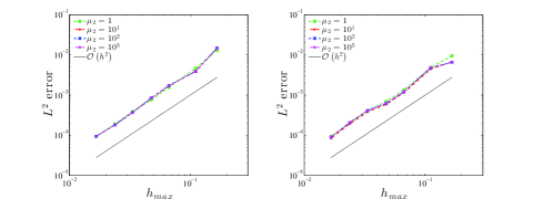
Fig. 7: Piecewise affine approximation, $\mu_{1}=1$, left $\frac{h_{1}}{h_{2}}=1$, right $\frac{h_{1}}{h_{2}}=\frac{3}{5}$.

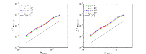
Fig. 8: Piecewise affine approximation, $\mu_{1}=1$, left $\frac{h_{1}}{h_{2}}=\frac{3}{10}$, right $\frac{h_{1}}{h_{2}}=\frac{1}{5}$.

Figure 7 and 8 shows a convergence of order $\mathcal{O}(h^{2})$ for the $L^{2}$-error, this is a super convergence of order $\mathcal{O}(h^{\frac{1}{2}})$ compared to the theoretical result. This super convergence has been observed for linear elasticity with the penalty free Nitsche’s method in [4]. Comparing all four graphs we observe that as the ratio $h_{1}/h_{2}$ becomes smaller the constant $C_{\mu}^{\prime}$ becomes slightly bigger when $\mu_{2}$ grows.

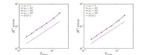
Fig. 9: Piecewise affine approximation, $\mu_{1}=1$, left $\frac{h_{1}}{h_{2}}=1$, right $\frac{h_{1}}{h_{2}}=\frac{3}{5}$.

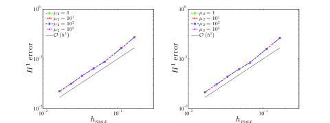
Fig. 10: Piecewise affine approximation, $\mu_{1}=1$, left $\frac{h_{1}}{h_{2}}=\frac{3}{10}$, right $\frac{h_{1}}{h_{2}}=\frac{1}{5}$.

We note that in all the cases the slope of convergence that has been proven theoretically is observed as it is shown in Figures 9 and 10. In fact the affine approximation considered gives slopes of convergence of order $\mathcal{O}\left(h\right)$ which is what has been shown theoretically. For $h_{1}/h_{2}=1$ the meshsize are the same on both sides of $\Gamma$, in this case the influence of $\mu_{2}$ is negligible, the error remains the same for every value of $\mu_{2}$ considered. By considering the ratio $h_{1}/h_{2}$ smaller, the nonconformity of the meshes on both size of gamma gets bigger but it has a very small impact on the error for the three nonconforming cases considered.

4.2 Unitted domain decomposition

The package FEniCS [19] and the library CutFEM [8] have been used for these computations.

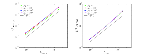
Fig. 11: Piecewise affine approximation, unfitted case, $\gamma_{g}=0.001$.

The same super convergence is observed as in the fitted case for the $L^{2}$-error. The case $\mu_{2}=1$ seems to have a constant $C_{f\mu}^{\prime}$ slightly smaller than the other cases. The $H^{1}$-error shows the same convergence as shown in the theory, once again, the difference between each case is negligible.

References

- [1] P. Angot, A unified fictitious domain model for general embedded boundary conditions, C. R. Math. Acad. Sci. Paris, 341 (2005), pp. 683–688.
- [2] N. Barrau, R. Becker, E. Dubach, and R. Luce, A robust variant of NXFEM for the interface problem, Comptes Rendus Mathematique, 350 (2012), pp. 789 – 792.
- [3] R. Becker, P. Hansbo, and R. Stenberg, A finite element method for domain decomposition with non-matching grids, M2AN Math. Model. Numer. Anal., 37 (2003), pp. 209–225.
- [4] T. Boiveau and E. Burman, A penalty free nitsche type method for the weak imposition of boundary conditions in compressible and incompressible elasticity, IMA J. Numer. Anal. (to appear), (2015).
- [5] T. Boiveau, E. Burman, and S. Claus, Fictitious domain method with penalty free nitsche type method, (preprint), (2015).
- [6] E. Burman, Ghost penalty, C. R. Math. Acad. Sci. Paris, 348 (2010), pp. 1217–1220.
- [7] , A penalty free nonsymmetric Nitsche-type method for the weak imposition of boundary conditions, SIAM J. Numer. Anal., 50 (2012), pp. 1959–1981.
- [8] E. Burman, S. Claus, P. Hansbo, M. G. Larson, and A. Massing, Cutfem: Discretizing geometry and partial differential equations, International Journal for Numerical Methods in Engineering, (2014), pp. n/a–n/a.
- [9] E. Burman and P. Hansbo, Fictitious domain finite element methods using cut elements: II. A stabilized Nitsche method, Appl. Numer. Math., 62 (2012), pp. 328–341.
- [10] E. Burman and P. Zunino, A domain decomposition method based on weighted interior penalties for advection-diffusion-reaction problems, SIAM J. Numer. Anal., 44 (2006), pp. 1612–1638 (electronic).
- [11] A. Ern, A. F. Stephansen, and P. Zunino, A discontinuous galerkin method with weighted averages for advection–diffusion equations with locally small and anisotropic diffusivity, IMA Journal of Numerical Analysis, 29 (2009), pp. 235–256.
- [12] J. Freund and R. Stenberg, On weakly imposed boundary conditions for second order problems, in Proceedings of the Ninth International Conference on Finite Elements in Fluids, Università di Padova, 1995, pp. 327–336.
- [13] V. Girault and R. Glowinski, Error analysis of a fictitious domain method applied to a dirichlet problem, Japan Journal of Industrial and Applied Mathematics, 12 (1995), pp. 487–514.
- [14] V. Girault, R. Glowinski, and T. W. Pan, A fictitious-domain method with distributed multiplier for the Stokes problem, in Applied nonlinear analysis, Kluwer/Plenum, New York, 1999, pp. 159–174.
- [15] A. Hansbo and P. Hansbo, An unfitted finite element method, based on Nitsche’s method, for elliptic interface problems, Comput. Methods Appl. Mech. Engrg., 191 (2002), pp. 5537–5552.
- [16] J. Haslinger and Y. Renard, A new fictitious domain approach inspired by the extended finite element method, SIAM Journal on Numerical Analysis, 47 (2009), pp. 1474–1499.
- [17] F. Hecht, New development in freefem++, J. Numer. Math., 20 (2012), pp. 251–265.
- [18] T. J. R. Hughes, G. Engel, L. Mazzei, and M. G. Larson, A comparison of discontinuous and continuous Galerkin methods based on error estimates, conservation, robustness and efficiency, in Discontinuous Galerkin methods (Newport, RI, 1999), vol. 11 of Lect. Notes Comput. Sci. Eng., Springer, Berlin, 2000, pp. 135–146.
- [19] A. Logg, K.-A. Mardal, and G. N. Wells, Automated solution of differential equations by the finite element method : The FEniCS book, Lecture Notes in Computational Science and Engineering, Springer, Berlin, Heidelberg, 2012.
- [20] A. Massing, M. G. Larson, A. Logg, and M. E. Rognes, A stabilized nitsche fictitious domain method for the stokes problem, Journal of Scientific Computing, 61 (2014), pp. 604–628.
- [21] J. Nitsche, Über ein variationsprinzip zur lösung von Dirichlet-problemen bei verwendung von teilräumen, die keinen randbedingungen unterworfen sind, Abhandlungen aus dem Mathematischen Seminar der Universität Hamburg, 36 (1971), pp. 9–15.