Stability Analysis of Sampled-Data Switched Systems
with Quantization

Abstract

We propose a stability analysis method for sampled-data switched linear systems with finite-level static quantizers. In the closed-loop system, information on the active mode of the plant is transmitted to the controller only at each sampling time. This limitation of switching information leads to a mode mismatch between the plant and the controller, and the system may become unstable. A mode mismatch also makes it difficult to find an attractor set to which the state trajectory converges. A switching condition for stability is characterized by the total time when the modes of the plant and the controller are different. Under the condition, we derive an ultimate bound on the state trajectories by using a common Lyapunov function computed from a randomized algorithm. The switching condition can be reduced to a dwell-time condition.

I Introduction

The recent advance of networking technologies makes control systems more flexible. However, the use of networks also raises new challenges such as packet dropouts, variable transmission delays, and real-time task scheduling. Switched system models provide a mathematical framework for such network properties because of their versatility to include both continuous flows and discrete jumps; see [16, 3, 41, 30] and references therein for the application of switched system models to networked control systems.

On the other hand, many control loops in a practical network contain channels over which only a finite number of bits can be transmitted. We need to quantize data before sending them out through a network. Therefore the effect of data quantization should be taken into consideration to achieve stability and desired performance. In addition to the practical motivation, literature such as [35, 31, 25, 27] has answered the theoretical question of how much information is necessary/sufficient for a given control problem.

Switched systems and quantized control have been studied extensively but separately; see, e.g., [12, 29, 17] for switched systems and [26, 10, 21] for quantized control. However, quantized control of switched systems has received increasing attention in recent years. For discrete-time Markovian jump linear systems, control problems with limited information have been studied in [24, 19, 18, 36, 37]. Also, our previous work [34] has investigated the output feedback stabilization of continuous-time switched systems under a slow-switching assumption. In most of the above studies, the switching behavior of the plant is available to the controller at all times.

In contrast, in sampled-data switched systems with quantization, the controller receives the quantized measurement and the active mode of the plant only at each sampling time. Since the controller side does not know the active mode of the plant between sampling times, we do not always use the controller mode consistent with the plant mode at the present time. The closed-loop system may therefore become unstable when switching occurs between sampling times. Moreover, for the stability of quantized systems, it is important to obtain regions to which the state belongs. However, mode mismatches yield complicated state trajectories, which make it difficult to find such regions.

Stabilization of sampled-data switched system with dynamic quantizers has been first addressed in [13], which has proposed an encoding strategy for state feedback control. This encoding method has been extended to the output feedback case [32] and to the case with disturbances [39]. A crucial ingredient in the dynamic quantization is a reachable set of the state trajectories through sampling intervals. Propagation of reachable sets is used to set the quantization values at the next sampling time, and the dynamic quantizer achieves increasingly higher precision as the state approaches the origin. On the other hand, we study the stability analysis of sampled-data switched systems with finite-level static quantizers. For such a closed-loop system, asymptotic stability cannot be guaranteed. The objective of the present paper is therefore to find an ultimate bound on the system trajectories as in the single-modal case, e.g., [9, 8, 5, 4]. Since frequent mode mismatches make the trajectories diverge, a certain switching condition is required for the existence of ultimate bounds.

As in [20] for switched systems with time delays, we here characterize switching behaviors by the total time when the controller mode is not synchronized with the plant one, which we call the total mismatch time. We derive a sufficient condition on the total mismatch time for the system to be stable, by using an upper bound on the error due to sampling and quantization. Moreover, an ultimate bound on the state trajectories is obtained under the switching condition. For the stability analysis, we use a common Lyapunov function that guarantees stability for all individual modes in the non-switched case. We find such Lyapunov functions in a computationally efficient and less conservative way by combining the randomized algorithms in [8, 15] together.

From the total mismatch time, we can obtain an asynchronous switching time ratio. If the controller mode is synchronized with the plant one, then the closed-loop system is stable. Otherwise, the system may be unstable. Hence the total mismatch time is a characterization similar to the total activation time ratio [40] between stable modes and unstable ones. The crucial difference is that the unstable modes we consider are caused by switching within sampling intervals. Using the dependence of the instability on the sampling period, we can reduce the switching condition on the total mismatch time to a dwell-time condition, which is widely used for the stability analysis of switched systems. In Section 4, we will discuss in detail the relationship between the total mismatch time and the dwell time of switching behaviors.

This paper is organized as follows. In Section 2, we present the closed-loop system, the information structure, and basic assumptions. In Section 3, we first investigate the growth rate of the common Lyapunov function in the case when switching occurs in a sampling interval. Next we derive an ultimate bound on the state, together with a sufficient condition on switching for stability. Section 4 is devoted to reduce the derived switching condition to a dwell-time condition. We illustrate the results through a numerical example in Section 5. Finally, concluding remarks are given in Section 6.

This paper is based on a conference paper [33]. In the conference version, some of the proofs were omitted due to space limitations. The present paper provides complete results on the stability analysis in addition to an illustrative numerical example. We also made structural improvements in this paper.

Notation
We denote by $\mathbb{Z}_{+}$ the set of non-negative integers $\{k\in\mathbb{Z}:~{}k\geq 0\}$. For a set $\Omega\subset\mathbb{R}^{\sf n}$, $\mathop{\rm Cl~{}\!}(\Omega)$, $\mathop{\rm Int~{}\!}(\Omega)$, and $\partial\Omega$ are its closure, interior, and boundary, respectively. For sets $\Omega_{1},\Omega_{2}$, let $\Omega_{1}\setminus\Omega_{2}$ be the relative complement of $\Omega_{2}$ in $\Omega_{1}$, i.e., $\Omega_{1}\setminus\Omega_{2}:=\{\omega\in\Omega_{1}:~{}\omega\not\in\Omega_{2}\}$.

Let $M^{\top}$ denote the transpose of a matrix $M\in\mathbb{R}^{\sf n\times m}$. The Euclidean norm of a vector $v\in\mathbb{R}^{\sf n}$ is defined by $\|v\|:=(v^{\top}v)^{1/2}$. For a matrix $M\in\mathbb{R}^{\sf m\times n}$, its Euclidean induced norm is defined by $\|M\|:=\sup\{\|Mv\|:~{}v\in\mathbb{R}^{\sf n},~{}\|v\|=1\}$. Let $\lambda_{\max}(P)$ and $\lambda_{\min}(P)$ denote the largest and the smallest eigenvalue of a square matrix $P\in\mathbb{R}^{\sf n\times n}$. Let $\mathcal{B}(L)$ be the closed ball in $\mathbb{R}^{\sf n}$ with center at the origin and radius $L$, that is, $\mathcal{B}(L):=\{x\in\mathbb{R}^{\sf n}:~{}\|x\|\leq L\}$.

Let $T_{s}$ be the sampling period. For $t\geq 0$, we define $[t]^{-}$ by

$$[t]^{-}:=kT_{s}\qquad\text{if~{}~{}~{}}kT_{s}\leq t<(k+1)T_{s}\qquad(k\in\mathbb{Z}_{+}).$$

II Sampled-data Switched Systems with Quantization

II-A Switched systems

Consider the following continuous-time switched linear system

$$\dot{x}=A_{\sigma}x+B_{\sigma}u,$$ (1)

where $x(t)\in\mathbb{R}^{\sf n}$ is the state and $u(t)\in\mathbb{R}^{\sf m}$ is the control input. For a finite index set $\mathcal{P}$, the mapping $\sigma:~{}[0,\infty)\to\mathcal{P}$ is right-continuous and piecewise constant, which indicates the active mode $\sigma(t)\in\mathcal{P}$ at each time $t\geq 0$. We call $\sigma$ a switching signal, and the discontinuities of $\sigma$ switching times or simply switches. The plant sends to the controller the state $x$ and the switching signal $\sigma$.

The first assumption is stabilizability of all modes.

Assumption II.1

For every mode $p\in\mathcal{P}$, $(A_{p},B_{p})$ is stabilizable, i.e., there exists a feedback gain $K_{p}\in\mathbb{R}^{\sf m\times n}$ such that $A_{p}+B_{p}K_{p}$ is Hurwitz.

II-B Quantized sampled-data system

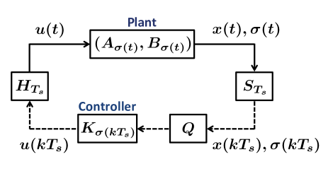
Figure 1: Sampled-data switched system with quantization, where $T_{s}$ is the sampling period and $S_{T_{s}}$, $H_{T_{s}}$, and $Q$ are a sampler, a zero-order hold, and a static quantizer, respectively.

Consider the closed-loop system in Fig. 1. Let $T_{s}>0$ be the sampling period. The sampler $S_{T_{s}}$ is given by

$$S_{T_{s}}:(x,\sigma)\mapsto(x(kT_{s}),\sigma(kT_{s}))\qquad(k\in\mathbb{Z}_{+}),$$

and the zero-order hold $H_{T_{s}}$ by

$$H_{T_{s}}\!:u_{d}\!\mapsto\!u(t)\!=\!u_{d}(k),~{}t\in[kT_{s},(k+1)T_{s})~{}~{}(k\in\mathbb{Z}_{+}).$$

The second assumption is that at most one switch happens in each sampling interval.

Assumption II.2

Every sampling interval $(kT_{s},(k+1)T_{s})$ has at most one switch.

See Remark II.5 (3) below for the reason why we need this switching assumption.

We now state the definition of a memoryless quantizer $Q$ given in [8]. For an index set $\mathcal{S}$, the partition $\{\mathcal{Q}_{j}\}_{j\in\mathcal{S}}$ of $\mathbb{R}^{\sf n}$ is said to be finite if for every bounded set $B$, there exists a finite subset $\mathcal{S}_{f}$ of $\mathcal{S}$ such that $B\subset\bigcup_{j\in\mathcal{S}_{f}}\mathcal{Q}_{j}$. We define the quantizer $Q$ with respect to the finite partition $\{\mathcal{Q}_{j}\}_{j\in\mathcal{S}}$ by

$$Q:~{}\mathbb{R}^{\sf n} \to\{q_{j}\}_{j\in\mathcal{S}}\subset\mathbb{R}^{\sf n}$$

$$x \mapsto q_{j}\quad\text{if~{}~{}}x\in\mathcal{Q}_{j}\quad(j\in\mathcal{S}).$$

As in [11, 14], we assume that $Q(x)=0$ if $x$ is close to the origin:

Assumption II.3

If $\mathop{\rm Cl~{}\!}(\mathcal{Q}_{j})$ contains the origin, then the corresponding quantization value $q_{j}=0$.

Let $q_{x}$ be the output of the zero-order hold whose input is the quantized state at sampling times, i.e., $q_{x}(t)=Q(x([t]^{-})).$ Note that in Fig. 1, the control input $u$ is given by

$$u(t)=K_{\sigma([t]^{-})}q_{x}(t).$$ (2)

The control input $u$ is a piecewise-constant and discrete-valued signal. If we assume that a finite subset $\mathcal{S}_{f}$ of $\mathcal{S}$ satisfies $x(t)\in\bigcup_{j\in\mathcal{S}_{f}}\mathcal{Q}_{j}$ for every state trajectory $x(t)$, then data is transmitted to/from the controller at the rate of

$$\frac{\log_{2}|\mathcal{S}_{f}|+\log_{2}|\mathcal{P}|}{T_{s}}$$

bits per time unit, where $|\mathcal{S}_{f}|$ and $|\mathcal{P}|$ are the numbers of elements in $\mathcal{S}_{f}$ and $\mathcal{P}$, respectively.

Let $P\in\mathbb{R}^{\sf n\times n}$ be positive definite and define the quadratic Lyapunov function $V(x):=x^{\top}Px$ for $x\in\mathbb{R}^{\sf n}$. Its time derivative $\dot{V}$ along the trajectory of (1) with (2) is given by

$$\dot{V}((t),q_{x}(t),\sigma(t))=(A_{\sigma(t)}x(t)+B_{\sigma(t)}K_{\sigma([t]^{-})} q_{x}(t))^{\top}Px(t)$$

$$+x(t)^{\top}P(A_{\sigma(t)}x(t)+B_{\sigma(t)}K_{\sigma([t]^{-})}q_{x}(t))$$ (3)

if $t$ is not a switching time or a sampling time.

For $p,q\in\mathcal{P}$ with $p\not=q$, we also define $\dot{V}_{p}$ and $\dot{V}_{p,q}$ by

$$\dot{V}_{p}(x(t),q_{x}(t)) :=(A_{p}x(t)+B_{p}K_{p}q_{x}(t))^{\top}Px(t)+x(t)^{\top}P(A_{p}x(t)+B_{p}K_{p}q_{x}(t))$$

$$\dot{V}_{p,q}(x(t),q_{x}(t)) :=(A_{p}x(t)+B_{p}K_{q}q_{x}(t))^{\top}Px(t)+x(t)^{\top}P(A_{p}x(t)+B_{p}K_{q}q_{x}(t)).$$ (4)

Then $\dot{V}_{p}$ and $\dot{V}_{p,q}$ are the time derivatives of $V$ along the trajectories of the systems $(A_{p},B_{p}K_{p})$ and $(A_{p},B_{p}K_{q})$, respectively.

Every individual mode is assumed to be stable in the following sense with the common Lyapunov function $V$:

Assumption II.4

Consider the following quantized sampled-data systems with ‘a single mode’:

$$\dot{x}=A_{p}x+B_{p}u,\quad u=K_{p}q_{x}\qquad(p\in\mathcal{P}).$$ (5)

Let $C$ be a positive number and suppose that $R$ and $r$ satisfy $R>r>0$. Then there exists a positive-definite matrix $P\in\mathbb{R}^{\sf n\times n}$ such that for all $p\in\mathcal{P}$, every trajectory $x$ of the system (5) with $x(0)\in\overline{\mathcal{E}}_{P}(R)$ satisfies

$$\dot{V}_{p}(x(t),q_{x}(t))\leq-C\|x(t)\|^{2}$$ (6)

or $x(t)\in\underline{\mathcal{E}}_{P}(r)$ for all $t\geq 0$, where $\overline{\mathcal{E}}_{P}(R)$ and $\underline{\mathcal{E}}_{P}(r)$ are given by

$$\overline{\mathcal{E}}_{P}(R) :=\{x\in\mathbb{R}^{\sf n}:~{}V(x)\leq R^{2}\lambda_{\max}(P)\}$$

$$\underline{\mathcal{E}}_{P}(r) :=\{x\in\mathbb{R}^{\sf n}:~{}V(x)\leq r^{2}\lambda_{\min}(P)\}.$$

Assumption II.4 implies the following: If we have no switches, then the common Lyapunov function $V$ exponentially decreases at a certain rate until $V\leq r^{2}\lambda_{\min}(P)$ for every mode $p\in\mathcal{P}$. Furthermore, the trajectory does not leave $\underline{\mathcal{E}}_{P}(r)$ as well as $\overline{\mathcal{E}}_{P}(R)$ once it falls into them.

The objective of the present paper is to find a switching condition under which every trajectory of the switched system in Fig. 1 falls into some neighborhood of the origin and remains in the neighborhood. We also determine how small the neighborhood is.

Remark II.5

(1) The ellipsoid $\overline{\mathcal{E}}_{P}(R)$ is the smallest level set of $V$ containing $\mathcal{B}(R)$, whereas $\underline{\mathcal{E}}_{P}(r)$ is the largest level set of $V$ contained in $\mathcal{B}(r)$.

(2) For switched systems without samplers, the existence of common Lyapunov functions is a sufficient condition for stability under arbitrary switching; see, e.g., [12, 17, 29]. For sampled-data switched systems, however, such functions do not guarantee stability because switching within a sampling interval may make the closed-loop system unstable.

(3) Not only sampling but also quantization makes the stability analysis complicated. In fact, Assumption II.4 does not consider trajectories after a switch even without a mode mismatch. For example, suppose that the mode changes $p\to q\to p$ at the switching times $t_{1}$ and $t_{2}$ in a sampling interval $(0,T_{s})$. Although the modes coincide between the plant and the controller in $[t_{2},T_{s})$, (6) holds only for $t\in(0,t_{1})$. This is because the trajectory in $[t_{2},T_{s})$ does not appear for systems with a single mode. In Assumption II.2, we therefore assume that at most one switch occurs in a sampling interval, and hence (6) holds whenever the modes coincide. If we consider trajectories in the worst case, then the switching condition in Assumption II.2 can be removed. However, the stability analysis becomes more conservative and involved.

(4) For quantized sampled-data plants with a single mode, the authors of [8] have proposed a randomized algorithm for the computation of $P$ in Assumption II.4. On the other hand, for switched systems without sampler or quantizer, the authors of [15] have developed a randomized algorithm to construct common Lyapunov functions. Combining these algorithms together, we can efficiently compute the desired common Lyapunov function. See Appendix B for details of the randomized algorithm.

III Stabilization with Limited Information

III-A Upper bound on $\dot{V}_{p,q}$

Assumption II.4 gives an upper bound (6) on $\dot{V}_{p}$, i.e., the decreasing rate of the Lyapunov function in the case when we use the feedback gain consistent with the currently active mode of the plant. In this subsection, we will find an upper bound on $\dot{V}_{p,q}$, i.e., the growth rate in the case when intersample switching leads to the mismatch of the modes between the plant and the feedback gain. More specifically, the aim here is to obtain $D>0$ satisfying

$$\dot{V}_{p,q}(x(t),q_{x}(t))\leq D\|x(t)\|^{2}.$$ (7)

Let $q_{x}(t)-x(t)$ is the error between the sampled and quantized state $q_{x}(t)$ and the state $x(t)$ at the present time. Since

$$\dot{V}_{p,q}(x(t),q_{x}(t)) =2x(t)^{\top}P(A_{p}+B_{p}K_{q})x(t)+2x(t)^{\top}PB_{p}K_{q}(q_{x}(t)-x(t)),$$ (8)

we need to obtain a bound on the error $q_{x}(t)-x(t)$ by using $x(t)$. We begin by examining the relationship among the state at the present time $x(t)$, the sampled state $x([t]^{-})$, and the sampled quantized state $q_{x}(t)$.

The partition $\{\mathcal{Q}_{j}\}_{j\in\mathcal{S}}$ is finite. Furthermore, Assumption II.3 shows that if there exists a sequence $\{\xi_{k}\}\subset\mathcal{Q}_{j}$ such that $\xi_{k}\to 0$ ($k\to\infty$), then $Q(x)=0$ for all $x\in\mathcal{Q}_{j}$. Hence there exists a constant $\alpha_{0}>0$ such that

$$\|B_{p}K_{q}Q(x)\|\leq\alpha_{0}\|x\|$$ (9)

for all $p,q\in\mathcal{P}$ and $x\in\overline{\mathcal{E}}_{P}(R)$; see Remark III.6 (3) for the computation of $\alpha_{0}$. We also define $\Lambda$ by

$$\Lambda:=\max_{p\in\mathcal{P}}\|A_{p}\|.$$

The next result gives an upper bound of the norm of the sampled state $x([t]^{-})$ by using the state at the present time $x(t)$.

Lemma III.1

Consider the swithced system (1) with (2), where $\sigma$ has finitely many switching times in every finite interval. Suppose that

$$\eta:=\alpha_{0}\frac{e^{\Lambda T_{s}}-1}{\Lambda}<1,$$ (10)

and define $\alpha_{1}$ by

$$\alpha_{1}:=\frac{e^{\Lambda T_{s}}}{1-\eta}.$$ (11)

Then we have

$$\|x([t]^{-})\|<\alpha_{1}\|x(t)\|$$ (12)

for all $t\geq 0$ with $x([t]^{-})\in\overline{\mathcal{E}}_{P}(R)$.

Proof: It suffices to prove (12) for $x(0)\in\overline{\mathcal{E}}_{P}(R)$ and $t\in[0,T_{s})$.

Let $\Phi(\tau_{1},\tau_{2})$ denote the state-transition matrix of the switched system (1) for $\tau_{1}\geq\tau_{2}$. If no switches occur, $\Phi(\tau_{1},\tau_{2})$ is given by $\Phi(\tau_{1},\tau_{2})=e^{(\tau_{1}-\tau_{2})A_{\sigma(\tau_{2})}}$. If $t_{1},t_{2},\dots,t_{m}$ are the switching times in an interval $(\tau_{2},\tau_{1})$ and if we define $t_{0}:=\tau_{2}$ and $t_{m+1}:=\tau_{1}$, then we have

$$\Phi(\tau_{1},\tau_{2})=\prod_{k=0}^{m}e^{(t_{k+1}-t_{k})A_{\sigma(t_{k})}}.$$

Since

$$x(t)=\Phi(t,0)x(0)+\int^{t}_{0}\Phi(t,\tau)B_{\sigma(\tau)}K_{\sigma(0)}q_{x}(\tau)d\tau$$ (13)

and since $\Phi(\tau,0)^{-1}=\Phi(t,0)^{-1}\Phi(t,\tau)$, it follows that

$$x(0)=\Phi(t,0)^{-1}x(t)+\int^{t}_{0}\Phi(\tau,0)^{-1}B_{\sigma(\tau)}K_{\sigma(0)}q_{x}(\tau)d\tau.$$

This leads to

$$\|x(0)\|\leq \|\Phi(t,0)^{-1}\|\cdot\|x(t)\|+\left\|\int^{t}_{0}\Phi(\tau,0)^{-1}B_{\sigma(\tau)}K_{\sigma(0)}q_{x}(\tau)d\tau\right\|.$$ (14)

Let $t_{1},t_{2},\dots,t_{m}$ be the switching times in the interval $[0,t)$. Since $\|e^{\tau A}\|\leq e^{\tau\|A\|}$ for $\tau\geq 0$, if we define $t_{0}:=0$ and $t_{m+1}:=t$, then we obtain

$$\|\Phi(t,0)^{-1}\|\leq\prod_{k=0}^{m}e^{(t_{k+1}-t_{k})\|A_{\sigma(t_{k})}\|}\leq e^{\Lambda t}<e^{\Lambda T_{s}}.$$ (15)

It is obvious that the equation above holds in the non-switched case as well. Since $q_{x}(\tau)=q_{x}(0)=Q(x(0))$ for all $\tau\in[0,T_{s}]$, if follows from (9) that

$$\left\|\int^{t}_{0}\Phi(\tau,0)^{-1}B_{\sigma(\tau)}K_{\sigma(0)}q_{x}(\tau)d\tau\right\| \leq\int^{t}_{0}\|\Phi(\tau,0)^{-1}\|\cdot\|B_{\sigma(\tau)}K_{\sigma(0)}q_{x}(\tau)\|d\tau$$

$$\leq\alpha_{0}\int^{t}_{0}e^{\Lambda\tau}d\tau\|x(0)\|$$

$$\leq\alpha_{0}\frac{e^{\Lambda T_{s}}-1}{\Lambda}\|x(0)\|=\eta\|x(0)\|.$$ (16)

Substituting (15) and (16) into (14), we obtain

$$\|x(0)\|<e^{\Lambda T_{s}}\|x(t)\|+\eta\|x(0)\|.$$

Thus if (10) holds, (12) follows.  ∎

Let us next develop an upper bound of the norm of the error $x(t)-x([t]^{-})$ due to sampling. To this end, we use the following property of the state-transition map of a switched system:

Proposition III.2

Let $\Phi(t,0)$ be the state-transition map of the switched system (1) as above. Then

$$\|\Phi(t,0)-I\|\leq e^{\Lambda t}-1.$$ (17)

Proof: Let us first consider the case without switching; that is,

$$\|e^{tA_{\sigma(0)}}-I\|\leq e^{\Lambda t}-1.$$ (18)

Define the partial sum $S_{N}$ of $e^{tA_{\sigma(0)}}-I$ by

$$S_{N}(t):=\sum_{k=0}^{N}\frac{1}{k!}(tA_{\sigma(0)})^{k}-I=\sum_{k=1}^{N}\frac{1}{k!}(tA_{\sigma(0)})^{k}.$$

Then for all $t\geq 0$, we have

$$\|S_{N}(t)\| \leq\sum_{k=1}^{N}\frac{1}{k!}\left(t\|A_{\sigma(0)}\|\right)^{k}$$

$$=\sum_{k=0}^{N}\frac{1}{k!}\left(t\|A_{\sigma(0)}\|\right)^{k}-1$$

$$\leq\sum_{k=0}^{\infty}\frac{1}{k!}\left(t\|A_{\sigma(0)}\|\right)^{k}-1$$

$$=e^{t\|A_{\sigma(0)}\|}-1\leq e^{\Lambda t}-1.$$

Letting $N\to\infty$, we obtain (18).

We now prove (17) in the switched case. Let $t_{1},t_{2},\dots,t_{m}$ be the switching times in the interval $(0,t)$. Let $t_{0}=0$ and $t_{m+1}=t$. Then (17) is equivalent to

$$\left\|~{}\prod_{k=0}^{m}e^{(t_{k+1}-t_{k})A_{\sigma(t_{k})}}-I~{}\right\|\leq e^{\Lambda t}-1.$$ (19)

We have already shown (19) in the case $m=0$, i.e., the non-switched case. The general case follows by induction. For $m\geq 1$,

$$\left\|\prod_{k=0}^{m}e^{(t_{k+1}-t_{k})A_{\sigma(t_{k})}}-I\right\|$$

$$\qquad\leq\left\|e^{(t_{m+1}-t_{m})A_{\sigma(t_{m})}}\left(\prod_{k=0}^{m-1}e^{(t_{k+1}-t_{k})A_{\sigma(t_{k})}}-I\right)\right\|+\|e^{(t_{m+1}-t_{m})A_{\sigma(t_{m})}}-I\|$$

$$\qquad\leq\|e^{(t_{m+1}-t_{m})A_{\sigma(t_{m})}}\|\cdot\left\|\prod_{k=0}^{m-1}e^{(t_{k+1}-t_{k})A_{\sigma(t_{k})}}-I\right\|+\|e^{(t_{m+1}-t_{m})A_{\sigma(t_{m})}}-I\|.$$

Hence if (19) holds with $m-1$ in place of $m$, then

$$\|e^{(t_{m+1}-t_{m})A_{\sigma(t_{m})}}\|\cdot\left\|\prod_{k=0}^{m-1}e^{(t_{k+1}-t_{k})A_{\sigma(t_{k})}}\!-\!I\right\|+\|e^{(t_{m+1}-t_{m})A_{\sigma(t_{m})}}\!-\!I\|$$

$$\qquad\leq e^{\Lambda(t_{m+1}-t_{m})}(e^{\Lambda t_{m}}\!-\!1)+(e^{\Lambda(t_{m+1}-t_{m})}\!-\!1)$$

$$\qquad=e^{\Lambda t}-1.$$

Thus we obtain (19).  ∎

Lemma III.3

Consider the switched system (1) with (2), where $\sigma$ has finitely many switching times in every finite interval. Define $\beta_{1}$ by

$$\beta_{1}:=(e^{\Lambda T_{s}}-1)\left(1+\frac{\alpha_{0}}{\Lambda}\right)$$ (20)

Then we have

$$\|x(t)-x([t]^{-})\|<\beta_{1}\|x([t]^{-})\|$$ (21)

for all $t\geq 0$ with $x([t]^{-})\in\overline{\mathcal{E}}_{P}(R)$.

Proof: As in the proof of Lemma III.1, it suffices to prove (21) for all $x(0)\in\overline{\mathcal{E}}_{P}(R)$ and $t\in[0,T_{s})$.

By (13), we obtain

$$x(t)-x(0)=(\Phi(t,0) -I)x(0)+\int^{t}_{0}\Phi(t,\tau)B_{\sigma(\tau)}K_{\sigma(0)}q_{x}(\tau)d\tau.$$

This leads to

$$\|x(t)-x(0)\|\leq \|\Phi(t,0)-I\|\cdot\|x(0)\|+\left\|\int^{t}_{0}\Phi(t,\tau)B_{\sigma(\tau)}K_{\sigma(0)}q_{x}(\tau)d\tau\right\|.$$ (22)

Proposition III.2 provides the following upper bound on the first term of the right-hand side of (22):

$$\|\Phi(t,0)-I\|\leq e^{\Lambda t}-1<e^{\Lambda T_{s}}-1.$$ (23)

Since $\|\Phi(t,\tau)\|\leq e^{\Lambda(t-\tau)}$, a calculation similar to (16) gives

$$\left\|\int^{t}_{0}\Phi(t,\tau)B_{\sigma(\tau)}K_{\sigma(0)}q_{x}(\tau)d\tau\right\| \leq\alpha_{0}\frac{e^{\Lambda T_{s}}-1}{\Lambda}\|x(0)\|.$$ (24)

We obtain (21) by substituting (23) and (24) into (22).  ∎

We are now in the position to obtain an upper bound of the norm of the error $q_{x}(t)-x(t)$ due to sampling and quantization by using the original state $x(t)$.

Similarly to (9), to each $p,q\in\mathcal{P}$ with $p\not=q$, there corresponds a positive number $\gamma_{0}(p,q)$ such that

$$\|PB_{p}K_{q}(Q(x)-x)\| \leq\gamma_{0}(p,q)\|x\|$$ (25)

for all $x\in\overline{\mathcal{E}}_{P}(R)$; see Remark III.6 (3) for the computation of $\gamma_{0}$.

Lemma III.4

Consider the switched system (1) with (2), where $\sigma$ has finitely many switching times in every finite interval. Define $\alpha_{1}$ and $\beta_{1}$ as in Lemmas III.1 and III.3. If $\gamma(p,q)$ is defined by

$$\gamma(p,q) :=\alpha_{1}(\beta_{1}\|PB_{p}K_{q}\|+\gamma_{0}(p,q))$$ (26)

for each $p,q\in\mathcal{P}$ with $p\not=q$, then $\gamma(p,q)$ satisfies

$$\|PB_{p}K_{q}(q_{x}(t)-x(t))\| <\gamma(p,q)\|x(t)\|$$ (27)

for all $t\geq 0$ with $x([t]^{-})\in\overline{\mathcal{E}}_{P}(R)$.

Proof: Since $q_{x}(t)=Q(x([t]^{-}))$, it follows from (21) and (25) that

$$\|PB_{p}K_{q}(q_{x}(t)-x(t))\| \leq\|PB_{p}K_{q}(q_{x}(t)-x([t]^{-}))\|+\|PB_{p}K_{q}\|\cdot\|x([t]^{-})-x(t)\|$$

$$<(\beta_{1}\|PB_{p}K_{q}\|+\gamma_{0}(p,q))\|x([t]^{-})\|$$

$$<\alpha_{1}(\beta_{1}\|PB_{p}K_{q}\|+\gamma_{0}(p,q))\|x(t)\|.$$

Thus the desired inequality (27) holds.  ∎

Finally, the following theorem gives the growth rate of $V$ in the case when the modes of the plant and the controller are not synchronized.

Theorem III.5

Consider the switched system (1) with (2), where $\sigma$ has finitely many switching times in every finite interval. Using $\gamma(p,q)$ in (26), we define $D$ by

$$D:=2\max_{p\not=q}(\|P(A_{p}+B_{p}K_{q})\|+\gamma(p,q)).$$ (28)

Then (7) holds for every $p,q\in\mathcal{P}$ with $p\not=q$ and for every $t\geq 0$ with $x([t]^{-})\in\overline{\mathcal{E}}_{P}(R)$.

Proof: Since $\dot{V}_{p,q}$ satisfies (8), Lemma III.4 shows that

$$\dot{V}_{p,q}(x(t),q_{x}(t))\leq 2(\|P(A_{p}+B_{p}K_{q})\|+\gamma(p,q))\|x(t)\|^{2}$$ (29)

for all $p,q\in\mathcal{P}$ with $p\not=q$ and for all $t\geq 0$ with $x([t]^{-})\in\overline{\mathcal{E}}_{P}(R)$. Thus we obtain the desired result (7).  ∎

Remark III.6

(1) Fine quantization and fast sampling make $\alpha_{1}$ in (11), $\beta_{1}$ in (20), and $\gamma_{0}(p,q)$ in (25) small, which leads to a decrease of $D$ in (28).

(2) In this subsection, we have assumed that finitely many switches occurs in a sampling interval, which makes (15), (23), and (24) conservative. If we allow a higher computational cost, then another possibility of $\alpha_{1}$ in (11) and $\beta_{1}$ in (20) under Assumption II.2 would be

$$\alpha_{1} \!=\!\max_{p\not=q}\max_{0\leq t\leq T_{s}}\max_{0\leq t^{\prime}\leq t}\frac{\|e^{-A_{p}t^{\prime}}e^{-A_{q}(t-t^{\prime})}\|}{1-\alpha_{0}\left(\int^{t}_{t^{\prime}}\|e^{-A_{p}t^{\prime}}e^{-A_{q}(\tau-t^{\prime})}\|d\tau+\int^{t^{\prime}}_{0}\|e^{-A_{p}\tau}\|d\tau\right)}$$

$$\beta_{1} \!=\!\max_{p\not=q}\max_{0\leq t\leq T_{s}}\max_{0\leq t^{\prime}\leq t}\Biggl{(}\!\|e^{A_{q}(t-t^{\prime})}e^{A_{p}t^{\prime}}\!-\!I\|+\!\alpha_{0}\Biggl{(}\int^{t}_{t^{\prime}}\|e^{A_{q}(t-\tau)}\|d\tau+\!\!\int^{t^{\prime}}_{0}\|e^{A_{q}(t-t^{\prime})}e^{A_{p}(t^{\prime}-\tau)}d\tau\|\Biggr{)}\!\!\Biggr{)}\!,$$

where $t^{\prime}$ is a switching time in $[0,t]$.

(3) We can derive $\alpha_{0}$ in (9) and $\gamma_{0}(p,q)$ in (25) as follows. Let $\mathcal{S}_{f}$ be a subset of $\mathcal{S}$ such that $\overline{\mathcal{E}}_{P}(R)\subset\bigcup_{j\in\mathcal{S}_{f}}\mathcal{Q}_{j}$. Then

$$\alpha_{0}:=\max_{p,q\in\mathcal{P}}\max_{j\in\mathcal{S}_{f}}\frac{\|B_{p}K_{q}q_{j}\|}{\min_{x\in\mathcal{Q}_{j}}\|x\|}$$

satisfies (9). Note that if $\mathcal{Q}_{j}$ is a polyhedron, then $\min_{x\in\mathcal{Q}_{j}}\|x\|$ can be computed by quadratic programming; see, e.g, [1]. As regards $\gamma_{0}(p,q)$ in (25), define $\mathcal{S}_{0}:=\{j\in\mathcal{S}:~{}0\in\mathop{\rm Cl~{}\!}(\mathcal{Q}_{j})\}$. Since $Q(x)=0$ for $x\in\mathcal{Q}_{j}$ with $j\in\mathcal{S}_{0}$ by Assumption II.3, it follows that $\gamma_{0}(p,q)\geq\|PB_{p}K_{q}\|$. On the other hand, for $j\not\in\mathcal{S}_{0}$, we define $\hat{\gamma}_{0}$ by

$$\hat{\gamma}_{0}(p,q):=\max_{j\in\mathcal{S}_{f}\setminus\mathcal{S}_{0}}\frac{\|PB_{p}K_{q}\|\cdot\max_{x\in\mathcal{Q}_{j}}\|q_{j}-x\|}{\min_{x\in\mathcal{Q}_{j}}\|x\|}.$$

Since

$$\frac{\|PB_{p}K_{q}\|\cdot\max_{x\in\mathcal{Q}_{j}}\|q_{j}-x\|}{\min_{x\in\mathcal{Q}_{j}}\|x\|} \geq\frac{\|PB_{p}K_{q}\|\cdot\|q_{j}-x\|}{\|x\|}$$

$$\geq\frac{\|PB_{p}K_{q}(q_{j}-x)\|}{\|x\|},$$

$\gamma_{0}(p,q):=\max\{\|PB_{p}K_{q}\|,~{}\hat{\gamma}_{0}(p,q)\}$ satisfies (25). We can easily compute $\max_{x\in\mathcal{Q}_{j}}\|q_{j}-x\|$ if $\mathcal{Q}_{j}$ is a cuboid and $q_{j}$ is a center of a vertex of $\mathcal{Q}_{j}$. In fact, let the set of the vertices of $\mathcal{Q}_{j}$ be $\mathcal{V}_{j}$. Then $\max_{x\in\mathcal{Q}_{j}}\|q_{j}-x\|=\max_{x\in\mathcal{V}_{j}}\|q_{j}-x\|$, which implies that $\max_{x\in\mathcal{Q}_{j}}\|q_{j}-x\|$ can be obtained by calculating $\|q_{j}-v\|$ for all $v\in\mathcal{V}_{j}$.

III-B Stability analysis with total mismatch time

Let us analyze the stability of the switched system (1) with (2) by using the two upper bounds (6) and (7) of $\dot{V}$. Note that the former bound (6) is for the case $\sigma(t)=\sigma([t]^{-})$, while the latter (7) for the case $\sigma(t)\not=\sigma([t]^{-})$. As in [20] for switched systems with time delays, it is therefore useful to characterize switching signals by asynchronous periods.

Definition III.7

For $\tau_{1}>\tau_{2}\geq 0$, we define the total mismatch time $\mu(\tau_{1},\tau_{2})$ by the time in which the modes mismatch between the plant and the controller, that is,

$$\mu(\tau_{1},\tau_{2}):=\text{ the length of the set~{}}\{\tau\in[\tau_{2},\tau_{1}):\sigma(\tau)\not=\sigma([\tau]^{-})\}.$$ (30)

More explicitly, the length of a set in $\mathbb{R}$ means its Lebesgue measure. We shall not, however, use any measure theory because $\sigma$ has only finitely many discontinuities in every interval. We see that if the total mismatch time is small on average as the average dwell-time condition introduced in [7], then the system is stable. We also derive an ultimate bound on the state trajectories by using this characterization of switching signals.

Define $C_{P}$ and $D_{P}$ by

$$C_{P}:=\frac{C}{\lambda_{\max}(P)},\quad D_{P}:=\frac{D}{\lambda_{\min}(P)}.$$

The objective of this subsection is to prove the following theorem:

Theorem III.8

Let Assumptions II.1, II.2, II.3, and II.4 hold. Suppose that $L\geq 0$ satisfies

$$L<\frac{C_{P}}{C_{P}+D_{P}},$$ (31)

and that $\kappa>1$ satisfies

$$\kappa^{2}r^{2}\lambda_{\min}(P)<R^{2}\lambda_{\max}(P).$$ (32)

Define $f(\kappa)$ by

$$f(\kappa):=\frac{2\log\kappa}{C_{P}+D_{P}}.$$ (33)

If $\mu$ in (30) satisfies

$$\mu(t,0)\leq Lt$$ (34)

for every $t>0$, and for each $T_{0}\geq 0$ with $\sigma(T_{0})\not=\sigma([T_{0}]^{-})$

$$\mu(t,T_{0})\leq f(\kappa)+L(t-T_{0})$$ (35)

for every $t>T_{0}$, then there exists $T_{r}\geq 0$ such that for each $x(0)\in\mathop{\rm Int~{}\!}(\overline{\mathcal{E}}_{P}(R))$ and $\sigma(0)\in\mathcal{P}$, $x(t)\in\mathop{\rm Int~{}\!}(\underline{\mathcal{E}}_{P}(\kappa r))$ for all $t\geq T_{r}$. Furthermore, $x(t)\in\mathop{\rm Int~{}\!}(\overline{\mathcal{E}}_{P}(R))$ for all $t\geq 0$.

Remark III.9

(1) Theorem III.8 gives the stability analysis of the switched system by using the total mismatch time of the modes between the plant and the feedback gain. If a mismatch does occur, the closed-loop system may be unstable; otherwise it is stable. Our proposed method is therefore similar to that in [40], where the stability analysis of switched systems with stable and unstable subsystems is discussed with the aid of the total activation time ratio between stable subsystems and unstable ones. In [40], the average dwell time [7] is also required to be sufficiently large. However, such a condition is not needed here because we use a common Lyapunov function. Conditions on the total activation time ratio has been used for nonlinear systems in [23, 22, 38]. Moreover, this switching characterization has been applied to stabilization of systems with control inputs missing in [41] and to resilient control under denial-of-service attacks in [2].

(2) Although Theorem III.8 requires that (35) holds for each $T_{0}\geq 0$ with $\sigma(T_{0})\not=\sigma([T_{0}]^{-})$, it is enough to verify (35) only with the sampling instant $[T_{0}]^{-}+T_{s}$ in place of $T_{0}$. In fact, since at most one switch occurs in $[[T_{0}]^{-},[T_{0}]^{-}+T_{s})$, it follows that if $\sigma(T_{0})\not=\sigma([T_{0}]^{-})$, then

$$\mu(t,[T_{0}]^{-}+T_{s})=\mu(t,T_{0})-([T_{0}]^{-}+T_{s}-T_{0}).$$

Hence (35) holds for $t>T_{0}$ if it does for $t\geq[T_{0}]^{-}+T_{s}$.

First we study the state behavior that is outside of $\underline{\mathcal{E}}_{P}(r)$. The following lemma shows that every trajectory whose initial state is in $\mathop{\rm Int~{}\!}(\overline{\mathcal{E}}_{P}(R))$ falls into $\underline{\mathcal{E}}_{P}(r)$ if the total mismatch time $\mu$ is small on average. See also Fig. 2.

Lemma III.10

Let Assumptions II.1, II.2, II.3, and II.4 hold, and let $L\geq 0$ satisfy (31). If $\mu(t,0)$ achieves (34) for all $t>0$, then there exists $T_{r}\geq 0$ such that $x(T_{r})\in\underline{\mathcal{E}}_{P}(r)$ for every $x(0)\in\mathop{\rm Int~{}\!}(\overline{\mathcal{E}}_{P}(R))$ and $\sigma(0)\in\mathcal{P}$, and furthermore $x(t)\in\mathop{\rm Int~{}\!}(\overline{\mathcal{E}}_{P}(R))$ for all $t\in[0,T_{r}]$.

Proof: First we show that the trajectory $x(t)$ does not leave $\mathop{\rm Int~{}\!}(\overline{\mathcal{E}}_{P}(R))$ without belonging to $\underline{\mathcal{E}}_{P}(r)$. Namely, there does not exist $T_{R}>0$ such that

$$x(T_{R})\in\partial\overline{\mathcal{E}}_{P}(R),\quad\text{and}$$ (36)

$$x(t)\in\mathop{\rm Int~{}\!}(\overline{\mathcal{E}}_{P}(R))\setminus\underline{\mathcal{E}}_{P}(r)\qquad(0\leq t<T_{R}).$$ (37)

Assume, to reach a contradiction, (36) and (37) hold for some $T_{R}>0$. Recall that

$$\lambda_{\min}(P)\|x\|^{2}\leq V(x)=x^{\top}Px\leq\lambda_{\max}(P)\|x\|^{2}$$

for $x\in\mathbb{R}^{\sf n}$. It follows from (6) and (7) that

$$\begin{array}[]{c}\dot{V}_{p}(x(t),q_{x}(t))\leq-C_{P}V(x(t))\\[4.0pt] \dot{V}_{p,q}(x(t),q_{x}(t))\leq D_{P}V(x(t)).\end{array}$$ (40)

By (37) and (40), a successive calculation at each switching time shows that

$$V(x(T_{R})) \leq\exp\big{(}D_{P}\mu(T_{R},0)-C_{P}(T_{R}-\mu(T_{R},0))\big{)}V(x(0)).$$ (41)

Since (34) gives

$$D_{P}\mu(t,0)-C_{P}(t-\mu(t,0))\leq\left(\left(C_{P}+D_{P}\right)L-C_{P}\right)t$$ (42)

for all $t>0$, it follows from (31) and $x(0)\in\mathop{\rm Int~{}\!}(\overline{\mathcal{E}}_{P}(R))$ that

$$V(x(T_{R}))<V(x(0))<R^{2}\lambda_{\max}(P).$$

However, (36) shows that $V(x(T_{R}))=R^{2}\lambda_{\max}(P),$ and we have a contradiction.

Let us next prove that $x(T_{r})\in\underline{\mathcal{E}}_{P}(r)$ for some $T_{r}\geq 0$.

Suppose $x(t)\not\in\underline{\mathcal{E}}_{P}(r)$ for all $t\geq 0$. Then since the discussion above shows that $x(t)\in\mathop{\rm Int~{}\!}(\overline{\mathcal{E}}_{P}(R))\setminus\underline{\mathcal{E}}_{P}(r)$ for all $t\geq 0$, we obtain (41) with arbitrary $t\geq 0$ in place of $T_{R}$. Hence (31) and (42) show that $V(x(t))\to 0$ as $t\to\infty$. However, this contradicts $x(t)\not\in\underline{\mathcal{E}}_{P}(r)$, i.e., $V(x(t))>r^{2}\lambda_{\min}(P)>0$. Thus there exists $T_{r}\geq 0$ such that $x(T_{r})\in\underline{\mathcal{E}}_{P}(r)$.  ∎

From the next result, we see that the trajectory leaves $\underline{\mathcal{E}}_{P}(r)$ only if a switch occurs between sampling times. This is intuitively obvious because as mentioned in [8], $\underline{\mathcal{E}}_{P}(r)$ is an invariant set if a mode mismatch does not occur.

Lemma III.11

Let Assumptions II.1, II.2, II.3, and II.4 hold. If the trajectory $x(t)$ leaves $\underline{\mathcal{E}}_{P}(r)$ at $t=T_{0}$, more precisely, if there exists $\delta>0$ such that

$$x(T_{0})\in\partial\underline{\mathcal{E}}_{P}(r),~{}x(T_{0}+\varepsilon)\not\in\underline{\mathcal{E}}_{P}(r)~{}~{}~{}~{}(0<\varepsilon<\delta),$$ (43)

then $\sigma(T_{0})\not=\sigma([T_{0}]^{-})$.

Proof: Assume, to get a contradiction, that $\sigma(T_{0})=\sigma([T_{0}]^{-})$. Suppose that $\sigma(T)\not=\sigma([T]^{-})$ for some $T>T_{0}$. Let $T_{1}$ be the smallest number of such $T$. Define an interval $I_{\delta}$ by

$$I_{\delta}:=(0,\min\{\delta,T_{1}-T_{0}\}).$$

If there does not exist $T>T_{0}$ with $\sigma(T)\not=\sigma([T]^{-})$, then we define $I_{\delta}$ by $I_{\delta}:=(0,\delta)$. Since $V(x(t))$ is differentiable at all $t\geq 0$ except for sampling times and switching times, there is no loss of generality in assuming that $V(x(t))$ is differentiable in $I_{\delta}$. Since $\sigma(T_{0}+\varepsilon)=\sigma([T_{0}+\varepsilon]^{-})=\sigma([T_{0}]^{-})$ for all $\varepsilon\in I_{\delta}$, it follows from (6) that

$$\dot{V}(x(T_{0}+\varepsilon))\leq-C\|x((T_{0}+\varepsilon))\|^{2}\leq 0\qquad(\varepsilon\in I_{\delta}).$$

However, (43) gives

$$V(x(T_{0}+\varepsilon))>r^{2}\lambda_{\min}(P)=V(x(T_{0}))\qquad(\varepsilon\in I_{\delta}).$$

Since $V(x(t))$ is continuous, we have a contradiction by the mean value theorem. Thus $\sigma(T_{0})\not=\sigma([T_{0}]^{-})$.  ∎

Lemma III.12 below shows that the trajectory stays in a slightly larger ellipsoid than $\underline{\mathcal{E}}_{P}(r)$ after the trajectory enters into $\underline{\mathcal{E}}_{P}(r)$; see Fig. 2.

Lemma III.12

Let Assumptions II.1, II.2, II.3, and II.4 hold. Suppose that $T_{0}\geq 0$ is a time at which $x(t)$ leaves $\underline{\mathcal{E}}_{P}(r)$. Let $\kappa>1$ satisfy (32) and define $f(\kappa)$ by (33). Pick $L\geq 0$ with (31). If $\mu(t,T_{0})$ satisfies (35) for all $t>T_{0}$, then for every $\sigma(T_{0})\in\mathcal{P}$, there exists $T_{1}>T_{0}$ such that $x(T_{1})\in\underline{\mathcal{E}}_{P}(r)$, and furthermore $x(t)\in\mathop{\rm Int~{}\!}(\underline{\mathcal{E}}_{P}(\kappa r))$ for all $t\in[T_{0},T_{1}]$.

Proof: By (35), $V(x(t))$ satisfies

$$V(x(t))\leq\exp\big{(}\left(\left(C_{P}+D_{P}\right)L-C_{P}\right)(t-T_{0})\big{)}\cdot\exp\big{(}\left(C_{P}+D_{P}\right)f(\kappa)\big{)}V(x(T_{0}))$$ (44)

if $t>T_{0}$ satisfies $x(t^{\prime})\in\overline{\mathcal{E}}_{P}(R)\setminus\underline{\mathcal{E}}_{P}(r)$ for all $t^{\prime}\in(T_{0},t]$. On the other hand, since $x(T_{0})\in\partial\underline{\mathcal{E}}_{P}(r)$, it follows from (33) that

$$\exp\big{(}\left(C_{P}+D_{P}\right)f(\kappa)\big{)}V(x(T_{0}))=\kappa^{2}r^{2}\lambda_{\min}(P).$$ (45)

In conjunction with (32), this leads to

$$\exp\big{(}\left(C_{P}+D_{P}\right)f(\kappa)\big{)}V(x(T_{0}))<R_{2}\lambda_{\max}(P).$$

Hence we have $x(T_{1})\in\underline{\mathcal{E}}_{P}(r)$ for some $T_{1}>T_{0}$ from (31) and (44) as in the proof of Lemma III.10. Substituting (45) into (44), we also obtain $V(x(t))<\kappa^{2}r^{2}\lambda_{\min}(P)$ for $t\geq T_{0}$. Thus $x(t)\in\mathop{\rm Int~{}\!}(\underline{\mathcal{E}}_{P}(\kappa r))$ for $t\in[T_{0},T_{1}]$.  ∎

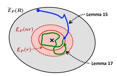
Figure 2: Behavior of trajectory

Finally, we prove Theorem III.8 by using Lemmas III.10, III.11, and III.12:

Proof of Theorem 3.8: Lemma III.10 shows that if (34) holds for all $t>0$, then $x(T_{r})\in\underline{\mathcal{E}}_{P}(r)$ for some $T_{r}>0$ and $x(t)\in\mathop{\rm Int~{}\!}(\overline{\mathcal{E}}_{P}(R))$ for all $t\in[0,T_{r}]$. Let $\tau_{1},\tau_{2},\dots$ be the instants at which $x(t)$ leaves $\underline{\mathcal{E}}_{P}(r)$. Using Lemmas III.11 and III.12 at each $\tau_{1},\tau_{2},\dots$, we have that if for each $T_{0}\geq 0$ with $\sigma(T_{0})\not=\sigma([T_{0}]^{-})$, (35) holds for every $t>T_{0}$, then there exists $\hat{\tau}_{k}\in(\tau_{k},\tau_{k+1}]$ such that $x(\hat{\tau}_{k})\in\underline{\mathcal{E}}_{P}(r)$ and $x(t)\in\mathop{\rm Int~{}\!}(\underline{\mathcal{E}}_{P}(\kappa r))$ for all $t\in[\tau_{k},\tau_{k+1}]$. Hence if $\{\tau_{k}\}$ has only finitely many elements, then the stability is achieved. On the other hand, if we have infinitely many $\tau_{k}$, then $\tau_{k}\to\infty$ as $k\to\infty$, because $\tau_{k+2}-\tau_{k}>T_{s}$ by the switching condition in Assumption II.2. Thus $x(t)\in\mathop{\rm Int~{}\!}(\underline{\mathcal{E}}_{P}(\kappa r))$ for all $t\geq T_{r}$. This completes the proof.  ∎

IV Reduction to a Dwell-Time Condition

In the preceding section, we have derived a sufficient condition on the total mismatch time $\mu$ for the stability of the quantized sampled-data systems with multiple modes. However, it may be difficult to check whether $\mu$ satisfies (34) and (35). In this section, we will show that these conditions (34) and (35) can be achieved for switching signals with a certain dwell-time property.

To proceed, we recall the definition of dwell time: We call $\sigma$ a switching signal with dwell time $T_{d}$ if the switching signal $\sigma$ has an interval between consecutive discontinuities no smaller than $T_{d}>0$ and further if $\sigma$ has no discontinuities in $[0,T_{d})$.

The following proposition gives an upper bound of the total mismatch time for switching signals with dwell time.

Proposition IV.1

Fix $n\in\mathbb{N}$. For every switching signal $\sigma$ with dwell time $nT_{s}$, $\mu$ in (30) satisfies

$$\mu(t,0)<\frac{t}{n}\qquad(t>0).$$ (46)

Furthermore, if $\sigma(T_{0})\not=\sigma([T_{0}]^{-})$, then

$$\mu(t,T_{0})<T_{s}+\frac{t-T_{0}}{n}\qquad(t>T_{0}).$$ (47)

Proof: The proof includes a lengthy but routine calculation; see Appendix A.1.  ∎

Theorem III.8 and Proposition IV.1 can be combined in the following way:

Theorem IV.2

Let Assumptions II.1, II.2, II.3, and II.4 hold. Let $n\in\mathbb{N}$ satisfy $n\geq 1+D_{P}/C_{P}$. Define

$$\kappa:=\exp\left(\frac{T_{s}(C_{P}+D_{P})}{2}\right),$$ (48)

and suppose that $\kappa$ satisfies (32). If the dwell time of $\sigma$ is $nT_{s}$, then there exists $T_{r}\geq 0$ such that for every $x(0)\in\mathop{\rm Int~{}\!}(\overline{\mathcal{E}}_{P}(R))$ and $\sigma(0)\in\mathcal{P}$, $x(t)\in\mathop{\rm Int~{}\!}(\underline{\mathcal{E}}_{P}(\kappa r))$ for all $t\geq T_{r}$. Furthermore, $x(t)\in\mathop{\rm Int~{}\!}(\overline{\mathcal{E}}_{P}(R))$ for all $t\geq 0$.

Proof: If $n$ and $\kappa$ are defined as above, Proposition IV.1 shows that $\mu$ satisfies (34) and (35) for every switching signal $\sigma$ with dwell time $nT_{s}$. Hence the conclusion of Theorem III.8 holds.  ∎

The next result implies that the upper bounds obtained in Proposition IV.1 are close to the supremum over all switching signals with dwell time $nT_{s}$ if the sampling period $T_{s}$ is sufficiently small.

Proposition IV.3

Fix $\varepsilon>0$ and $n\in\mathbb{N}$. For any $T\geq 0$, there exist a switching signal $\sigma$ with dwell time $nT_{s}$ and $t\geq T$ such that

$$\mu(t,0)\geq\frac{t}{n}-\left(\frac{T_{s}}{n}+\varepsilon\right).$$

Furthermore, for any $T\geq 0$, there exist a switching signal $\sigma$ with dwell time $nT_{s}$, $T_{0}\geq 0$ with $\sigma(T_{0})\not=\sigma([T_{0}]^{-})$, and $t\geq T_{0}+T$ such that

$$\mu(t,T_{0})\geq T_{s}+\frac{t-T_{0}}{n}-\left(\frac{T_{s}}{n}+\varepsilon\right).$$ (49)

Proof: This is again a routine calculation; see Appendix A.2.  ∎

The next result is the case $n=1$ in Proposition IV.3.

Corollary IV.4

There exist a switching signal $\sigma$ with dwell time $T_{s}$ such that $\mu(t,0)\approx t$ for sufficiently large $t>0$.

This corollary shows that, not surprisingly, if the dwell time does not exceed the sampling period, then the information on switching signals is not so useful for the stabilization of the sampled-data switched system.

V Numerical Example

Consider the switched system with the following two modes:

$$A_{1}=\frac{1}{6}\begin{bmatrix}1&-2\\ -3&2\end{bmatrix},\quad B_{1}=\frac{1}{6}\begin{bmatrix}-4\\ 3\end{bmatrix}$$

$$A_{2}=\begin{bmatrix}1&-5\\ 1&2\end{bmatrix},\quad B_{2}=\begin{bmatrix}1\\ -1\end{bmatrix}.$$

The state feedback gains $K_{1}$ and $K_{2}$ are given by

$$K_{1}=\begin{bmatrix}1.38&-1.86\end{bmatrix},\quad K_{2}=\begin{bmatrix}-2.80&3.77\end{bmatrix}.$$ (50)

We computed the above regulator gains by minimizing the cost

$$\int^{\infty}_{0}\big{(}x(t)^{\top}x(t)+u(t)^{2}\big{)}dt.$$

Note that both $A_{1}+B_{1}K_{2}$ and $A_{2}+B_{2}K_{1}$ are not Hurwitz: $A_{1}+B_{1}K_{2}$ has one unstable eigenvalue $4.4538$ and $A_{2}+B_{2}K_{1}$ has two unstable eigenvalues $1.4091$ and $4.7750$.

The sampling period $T_{s}$ was given by $T_{s}=0.025$, and we used the following logarithm quantizer: Let the state $x$ be $x=[x_{1}~{}~{}x_{2}]^{\top}$. For a nonnegative integer $n$, the quantized state $Q(x)=[Q_{1}(x_{1})~{}~{}Q_{2}(x_{2})]^{\top}$ is defined by

$$Q_{i}(x_{i}):=\begin{cases}\frac{-\xi_{0}(\eta^{n}+\eta^{n+1})}{2}&(-\xi_{0}\eta^{n+1}\leq x_{i}<-\xi_{0}\eta^{n})\\ 0&(-\xi_{0}\leq x_{i}\leq\xi_{0})\\ \frac{\xi_{0}(\eta^{n}+\eta^{n+1})}{2}&(\xi_{0}\eta^{n}<x\leq\xi_{0}\eta^{n+1}),\end{cases}$$

where $\xi_{0}=0.08$ and $\eta=1.2$.

Set $C=1$, $R=68.6$, and $r=0.175$ in Assumption II.4. Algorithm B.1 of Appendix B gave the positive definite matrix $P$ in Assumption II.4 by

$$P=\begin{bmatrix}2.9171&0.3489\\ 0.3489&3.6256\end{bmatrix}.$$

In the randomized algorithm, we used $10^{7}$ samples in state for each run, and five samples in time for each sampled state. We stopped the algorithm when there was no update for an entire run.

Since we obtain $D=55.15$ in (7) from the data above, the resulting $n$ and $\kappa$ in Theorem IV.2 are $n=76$ and $\kappa=1.2864$.

A time response ($0\leq t\leq 20$) was calculated for $\sigma(0)=1$ and some initial states on $\partial\overline{\mathcal{E}}_{P}(R-\epsilon)$ with $\epsilon=0.001$. Fig. 3 depicts the state trajectories $x$ of the switched system (1) with dwell time $76T_{s}=1.9$. After an interval of length $76T_{s}$ with no switches, a switch of the plant mode occurs with probability 0.05 per sampling interval and the distribution is uniform in a sampling interval. The blue line indicates that the feedback gain designed for the active subsystem was used, i.e.,

$$(A_{\sigma(t)},B_{\sigma(t)},K_{\sigma([t]^{-})})=(A_{1},B_{1},K_{1})~{}\text{or}~{}(A_{2},B_{2},K_{2}).$$

The red line shows that a switch led to the mismatch of the modes between the plant and the feedback gain, i.e.,

$$(A_{\sigma(t)},B_{\sigma(t)},K_{\sigma([t]^{-})})=(A_{1},B_{1},K_{2})~{}\text{or}~{}(A_{2},B_{2},K_{1}).$$

The black lines in Fig. 3 represent the ellipsoid of initial conditions $\overline{\mathcal{E}}_{P}(R)$ and the attractor set $\underline{\mathcal{E}}_{P}(\kappa r)$, respectively.

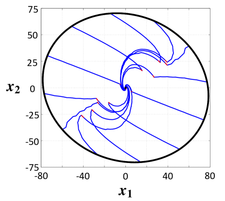
(a) Region $[-80,80]\times[-75,75]$

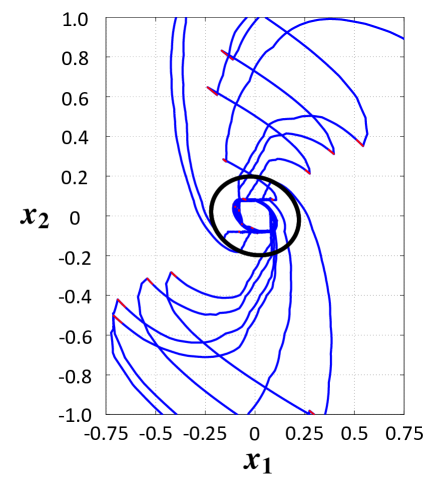
(b) Region $[-0.75,0.75]\times[-1.0,1.0]$

Figure 3: The trajectories $x$ with $\sigma(0)=1$

Here we see two conservative results: the dwell time $76T_{s}$ and the attractor set $\underline{\mathcal{E}}_{P}(\kappa r)$ in Fig. 3(b). Since we evaluate the increasing and decreasing rates of the Lyapunov function only by (7) and (6), the switching condition for stability becomes conservative. In particular, we need to refine the upper bound (7) in the mismatch case, which has been obtained by assuming that we have the worst-case trajectory whenever a mode mismatch occurs. If we know where switching happens as for piecewise affine systems, then the upper bound (7) can be improved.

As regards the attractor set $\underline{\mathcal{E}}_{P}(\kappa r)$, the trajectories in Fig. 3(b) stayed in a smaller neighborhood of the origin. The conservative result is also due to the upper bound (7); see (48). Another reason is the nonlinearity of static quantizers and this conservatism is observed for systems with a single mode as well [9, 8, 5]. Construction of polynomial Lyapunov functions may allow us to obtain less conservative bounds.

If we use multiple Lyapunov functions together with an average dwell-time property, instead of a common Lyapunov function, then the above conservatism can be reduced. On the other hand, the authors of [6] have proposed the calculation method of an ultimate bound and an invariant set for continuous-time switched systems with disturbances. If one can generalize this method to sampled-data switched systems with a static quantizer, then another insight into the state trajectory near the origin will be obtained. Details, however, are more involved, so these extensions are subjects for future research.

VI Concluding Remarks

For sampled-data switched systems with static quantizers, we have developed a stability analysis by using a common Lyapunov function computed efficiently from a randomized algorithm. We have derived a switching condition on the total mismatch time, and have found a neighborhood of the origin into which all trajectories fall whenever the initial state is within a known bound. Moreover, the condition on the total mismatch time has been reduced to a dwell-time condition. Future work will focus on improving the upper bound on the growth rate of the Lyapunov function in the mismatched case, and analyzing the stability by multiple Lyapunov functions and an average dwell-time property.

Appendix A Bound on Total Mismatch Time

A-A Proof of Proposition IV.1

Let us first prove (46). It is clear that $\mu=0$ if $\sigma$ has no discontinuities in the interval $(0,t)$. Let $t_{1},\dots,t_{m}$ be the switching times in $(0,t)$. We have

$$\mu([t_{k+1}]^{-},[t_{k}]^{-})=\begin{cases}[t_{k}]^{-}+T_{s}-t_{k}&\text{if $t_{k}\not=[t_{k}]^{-}$}\\ 0&\text{otherwise}\end{cases}$$

for $k=1,\dots,m-1$, and

$$\mu(t,[t_{m}]^{-})=\begin{cases}[t_{m}]^{-}+T_{s}-t_{m}&\text{if $t_{m}\not=[t_{m}]^{-}$ and $[t_{m}]^{-}+T_{s}<t$}\\ t-t_{m}&\text{if $t_{m}\not=[t_{m}]^{-}$ and $[t_{m}]^{-}+T_{s}\geq t$}\\ 0&\text{otherwise}\end{cases}$$

Since $t\geq mnT_{s}$, we obtain

$$\mu(t,0)\leq\sum_{k=1}^{m}([t_{k}]^{-}+T_{s}-t_{k})<mT_{s}\leq\frac{1}{n}t.$$

Hence (46) holds.

Next we show (47). Since $\sigma(T_{0})\not=\sigma([T_{0}]^{-})$ and since the dwell time is $nT_{s}\geq T_{s}$, it follows that $\sigma$ has precisely one discontinuity in the interval $([T_{0}]^{-},T_{0}]$. Let us denote the switching time by $t_{0}$.

Suppose that no switches occur in the interval $(T_{0},t)$. Since only the interval $[T_{0},[T_{0}]^{-}+T_{s})$ has a mode mismatch, it follows that

$$\mu(t,T_{0})\leq[T_{0}]^{-}+T_{s}-T_{0}<T_{s},$$

and hence (47) holds.

Suppose that $m$ switches occur in the interval $(T_{0},t)$, and let $t_{1},\dots,t_{m}$ be the switching times. Define $\xi_{k}$ by

$$\xi_{k}:=(t_{k+1}-t_{k})-nT_{s}$$ (51)

for $k=0,\dots,m-1$. The dwell-time assumption implies that $\xi_{k}\geq 0$. We also have

$$t-T_{0} =(t-t_{m})+\sum_{k=0}^{m-1}(t_{k+1}-t_{k})-(T_{0}-t_{0})$$

$$=(t-t_{m})+\sum_{k=0}^{m-1}(\xi_{k}+nT_{s})-(T_{0}-t_{0})$$

$$=mnT_{s}+(t-t_{m})+\sum_{k=0}^{m-1}\xi_{k}-(T_{0}-t_{0}).$$ (52)

We split the argument into two cases:

$$(t-t_{m})+\sum_{k=0}^{m-1}\xi_{k}\geq T_{0}-t_{0}$$ (53)

and

$$(t-t_{m})+\sum_{k=0}^{m-1}\xi_{k}<T_{0}-t_{0}.$$ (54)

First we study the case (53), where some switching intervals are sufficiently larger than $nT_{s}$. Combining (53) with (52), we obtain $t-T_{0}\geq mnT_{s}$, and hence

$$\mu(t,T_{0}) \leq([T_{0}]^{-}+T_{s}-T_{0})+\sum_{k=1}^{m}([t_{k}]^{-}+T_{s}-t_{k})$$

$$<(m+1)T_{s}\leq T_{s}+\frac{1}{n}(t-T_{0}),$$

which is a desired inequality (47).

Let us next consider the case (54), where every switching interval is smaller than $nT_{s}$. Since

$$\mu(t,T_{0})=\mu([t_{1}]^{-},T_{0}) +\sum_{k=1}^{m-1}\mu([t_{k+1}]^{-},[t_{k}]^{-})+\mu(t,[t_{m}]^{-})$$

and since $\mu([t_{1}]^{-},T_{0})=\mu([T_{0}]^{-}+T_{s},T_{0})\leq[T_{0}]^{-}+T_{s}-T_{0}$, it is enough to obtain upper bounds on $\mu([t_{k+1}]^{-},[t_{k}]^{-})$ and $\mu(t,[t_{m}]^{-})$.

We first derive

$$\mu([t_{k+1}]^{-},[t_{k}]^{-})\leq[t_{0}]^{-}+T_{s}-t_{0}$$ (55)

for $k=1,\dots,m-1$ as follows. Since $\sum_{k=0}^{m-1}\xi_{k}<T_{0}$ by (54), each switching time $t_{k}$ ($k=1,\dots,m$) satisfies

$$t_{k}-t_{0} =(t_{k}-t_{k-1})+\dots+(t_{1}-t_{0})$$

$$=\sum_{\ell=0}^{k-1}(\xi_{\ell}+nT_{s})$$

$$\leq\sum_{\ell=0}^{m-1}\xi_{\ell}+knT_{s}$$

$$<T_{0}-t_{0}+knT_{s}.$$

In conjunction with the assumption on the dwell time, this leads to

$$t_{0}+knT_{s}\leq t_{k}<T_{0}+knT_{s}$$ (56)

for every $k=1,\dots,m$. Since

$$[t_{0}]^{-}=[T_{0}]^{-}<t_{0}\leq T_{0}<[T_{0}]^{-}+T_{s},$$ (57)

(56) shows that $[t_{k}]^{-}=[t_{0}]^{-}+knT_{s}$, and hence

$$t_{0}+knT_{s}\leq t_{k}<[t_{k}]^{-}+T_{s}=[t_{0}]^{-}+knT_{s}+T_{s},$$

which gives $[t_{k}]^{-}+T_{s}-t_{k}\leq[t_{0}]^{-}+T_{s}-t_{0}$. We therefore have

$$\mu([t_{k+1}]^{-},[t_{k}]^{-}) =\mu([t_{k}]^{-}+T_{s},[t_{k}]^{-})$$

$$\leq[t_{k}]^{-}+T_{s}-t_{k}$$

$$\leq[t_{0}]^{-}+T_{s}-t_{0}.$$

Thus we obtain (55).

Similarly, we can obtain

$$\mu(t,[t_{m}]^{-})<T_{0}-t_{0}.$$ (58)

In fact, (54) and (51) give

$$t<(T_{0}-t_{0})+t_{m}-\sum_{k=0}^{m-1}\xi_{k}=T_{0}+mnT_{s}.$$

If we combine this with $t>t_{m}$ and (56), we see that

$$t_{0}+mnT_{s}\leq t_{m}<t<T_{0}+mnT_{s},$$

which implies that

$$\mu(t,[t_{m}]^{-})\leq t-t_{m}<T_{0}-t_{0}.$$

We therefore have (58).

Since $t-t_{m}>0$ and $\xi_{k}\geq 0$, it follows from (52) that $m$ satisfies $t-t_{0}>mnT_{s}$, i.e.,

$$m<\frac{t-t_{0}}{nT_{s}}.$$ (59)

By (55), (58), and (59), we have

$$\mu(t,T_{0}) <([T_{0}]^{-}+T_{s}-T_{0})+(m-1)([t_{0}]^{-}+T_{s}-t_{0})+(T_{0}-t_{0})$$

$$<\frac{t-t_{0}}{n}\frac{[t_{0}]^{-}+T_{s}-t_{0}}{T_{s}}$$

$$<\frac{t-[t_{0}]^{-}}{n}.$$ (60)

Moreover, (57) gives

$$T_{s}+\frac{t-T_{0}}{n}-\frac{t-[t_{0}]^{-}}{n} =T_{s}-\frac{T_{0}-[t_{0}]^{-}}{n}$$

$$>T_{s}-\frac{T_{s}}{n}\geq 0.$$

Hence (47) follows from (60).

A-B Proof of Proposition IV.3

Fix $T\geq 0$ and suppose that $m\in\mathbb{N}$ satisfies $mnT_{s}\geq T$.

To prove the first assertion of the theorem, let a switching signal $\sigma$ have discontinuities at $knT_{s}+\varepsilon/m$ $(k=1,\dots,m)$. If we define $t:=mnT_{s}+T_{s}$, then $t\geq T$ and we obtain

$$\mu(t,0)=m\left(T_{s}-\frac{\varepsilon}{m}\right)=mT_{s}-\varepsilon=\frac{t}{n}-\left(\frac{T_{s}}{n}+\varepsilon\right).$$

To prove the second assertion, let $T_{0}-[T_{0}]^{-}=\varepsilon/(2m+1)$ and let $\sigma$ have a switch at

$$T_{0}+knT_{s}+\frac{\varepsilon}{2(m+1)}=[T_{0}]^{-}+knT_{s}+\frac{\varepsilon}{m+1}.$$

for each $k=1,\dots,m$. If we set $t:=T_{0}+mnT_{s}+T_{s}$, then $t\geq T_{0}+T$ and we have

$$\mu(t,T_{0}) =\left(T_{s}-\frac{\varepsilon}{2(m+1)}\right)+m\left(T_{s}-\frac{\varepsilon}{m+1}\right)$$

$$\geq(m+1)T_{s}-\varepsilon$$

$$=T_{s}+\frac{t-T_{0}}{n}-\left(\frac{T_{s}}{n}+\varepsilon\right),$$

which is the desired inequality (49).

Appendix B Randomized Algorithm for Common Lypunov Functions

The randomized algorithm for the computation of $P$ in Assumption II.4 is summarized here for the sake of completeness.

For a square matrix $X\in\mathbb{R}^{\sf n\times n}$, we denote its Frobenius norm by $\|X\|_{F}=(\sum_{i,k=1}^{\sf n}x_{i,k}^{2})^{1/2}$, where $x_{i,k}$ is the $(i,k)$-th entry of $X$. For $X=X^{\top}\in\mathbb{R}^{\sf n\times n}$, let its eigenvalue decomposition be $X=U\Sigma U^{\top}$, where $U$ is orthogonal and $\Sigma=\text{diag}(\lambda_{1},\dots,\lambda_{\sf n})$. For a fixed $\gamma\geq 0$, define $\Sigma_{\gamma}:=\text{diag}(\max\{\lambda_{1},\gamma\},\dots,\max\{\lambda_{\sf n},\gamma\})$ and set $G_{\delta,\delta_{1}}(X):=U\Sigma_{\gamma}U^{\top}$, where $\gamma:=[(\delta^{2}-\delta^{2}_{1})/{\sf n}]^{1/2}$ for some $\delta>\delta_{1}>0$.

For the construction of common Lyapunov functions, we use a scheduling function $h:\mathbb{Z}_{+}\to\mathcal{P}$ that has the following revisitation property [15]: For every element $i\in\mathcal{P}$ and for every integer $l\in\mathbb{Z}_{+}$, there exists an integer $k\geq l$ such that $h(k)=i$.

We can construct the common Lyapunov function in Assumption II.4 by using the randomized algorithm of [8], which is based on the gradient method proposed in [28].

Algorithm B.1

(1)

Pick an initial $P^{[0,0]}>0$ and set $R_{0},r_{0},\delta>0$, and $\delta_{1}\in(0,\delta)$.

(2)

Find a finite index subset $\mathcal{S}_{N}$ of $\mathcal{S}$ such that $\mathcal{B}(R_{0})\subset\bigcup_{j\in\mathcal{S}_{N}}\mathcal{Q}_{j}$.

(3a)

Set $A:=A_{h(k)}$, $B:=B_{h(k)}$, and $K:=K_{h(k)}$, and define

$$\phi(x_{0},u,t) :=e^{At}x_{0}+\int^{t}_{0}e^{A\tau}Bd\tau\cdot u,$$

$$u_{j} :=Kq_{j}$$

$$v(P,x,j,t) :=(A\phi(x,u_{j},t)+Bu_{j})^{\top}P\phi(x,u_{j},t)$$

$$\qquad+\phi(x,u_{j},t)^{\top}P(A\phi(x,u_{j},t)+Bu_{j})+C\|\phi(x,u_{j},t)\|^{2}$$

$$\nabla_{P}v(P,x,j,t) :=(A\phi(x,u_{j},t)+Bu_{j})\phi(x,u_{j},t)^{\top}+\phi(x,u_{j},t)(A\phi(x,u_{j},t)+Bu_{j})^{\top}$$

$$\mathcal{X}_{P}(u) :=\{x\in\mathbb{R}^{\sf n}:~{}(Ax+Bu)^{\top}Px+x^{\top}P(Ax+Bu)\leq-C\|x\|^{2}\}.$$

(3b)

Generate

$$(x^{[k]},j^{[k]}) \in\{(x,j):x\in[\mathcal{Q}_{j}\cap(\partial\mathcal{B}(r_{0})\cup\partial\mathcal{B}(R_{0}))]\cup(\partial\mathcal{Q}_{j}\cap\mathcal{B}(R_{0})),~{}j\in\mathcal{S}_{N}\}$$

$$=:\mathcal{F}$$

according to some density function $f_{x,j}$ satisfying $f_{x,j}(x,j)>0$ for all $(x,j)\in\mathcal{F}$.

(3c)

If $x^{[k]}\in\partial\mathcal{B}(r_{0})\cup\partial\mathcal{B}(R_{0})$, then set

$$P^{[k+1,0]}=$$

$$\begin{cases}G_{\delta,\delta_{1}}(P^{[k,0]})-\mu^{[k,0]}\nabla v^{[k,0]}&\text{if $x^{[k]}\not\in\mathcal{X}_{P^{[k,0]}}(u_{j^{[k]}})$}\\ P^{[k,0]}&\text{otherwise},\end{cases}$$

where $\nabla v^{[k,0]}=\nabla_{P}v(P^{[k,0]},x^{[k]},j^{[k]},0)$ and $\mu^{[k,0]}$ is the step size given by

$$\mu^{[k,0]}:=\frac{v(P^{[k,0]},x^{[k]},j^{[k]},0)+\delta\|\nabla v^{[k,0]}\|_{F}}{\|\nabla v^{[k,0]}\|_{F}^{2}}.$$

(3d)

If $x^{[k]}\in\partial\mathcal{Q}_{j}\cap\mathcal{B}(R_{0})$, then

1. generate $\{t^{[k,i]}\}^{l-1}_{i=0}\subset[0,T_{s}]$ according to some density function $f_{t}$ satisfying $f_{t}(t)>0$ for all $t\in[0,T_{s}]$ with the indices in increasing order: $0\leq t^{[k,0]}<\dots<t^{[k,l-1]}\leq T_{s}$;

2. if $t^{[k,i]}\not=0$ and if $\phi(x^{[k]},u_{j^{[k]}},t^{[k,i]})\in\mathop{\rm Cl~{}\!}(\mathcal{Q}_{j^{[k]}}\cap\mathcal{B}(R_{0})^{c}\setminus\mathcal{B}(r_{0}))$, then set $P^{[k+1,0]}=P^{[k,i]}$; otherwise set

   $$P^{[k,i+1]}\!=\!\begin{cases}G_{\delta,\delta_{1}}(P^{[k,i]})\!-\!\mu^{[k,i]}\nabla v^{[k,i]}&\text{if $\phi(x^{[k]},u_{j^{[k]}},t^{[k,i]})\!\not\in\!\mathcal{X}_{P^{[k,0]}}(u_{j^{[k]}})\!\cup\!\mathcal{B}(R_{0})$}\\ P^{[k,i]}&\text{otherwise},\end{cases}$$

   where $\nabla v^{[k,i]}:=\nabla_{P}v(P^{[k,0]},x^{[k]},j^{[k]},t^{[k,i]})$ is the step size given by

   $$\mu^{[k,i]}:=\frac{v(P^{[k,0]},x^{[k]},j^{[k]},t^{[k,i]})+\delta\|\nabla v^{[k,i]}\|_{F}}{\|\nabla v^{[k,i]}\|_{F}^{2}};$$

3. set $P^{[k+1,0]}=P^{[k,l]}$.

(4)

Find $R>0$ satisfying $\overline{\mathcal{E}}_{P^{[k,0]}}(R)\subset\mathcal{B}(R_{0})$ and obtain $r>0$ satisfying $\mathcal{B}(r_{0})\subset\overline{\mathcal{E}}_{P^{[k,0]}}(r)\subset\overline{\mathcal{E}}_{P^{[k,0]}}(R)$ if it exists.

The major difference from the algorithm in [8] is the procedure (3a), where a scheduling function is used. Under assumptions similar to those in [8], we can show that Algorithm B.1 gives a solution in a finite number of steps with probability one. Since this is an immediate consequence of [8, 15], we omit the details.

References

• [1] S. Boyd and L. Vandenberghe. Convex Optimization. Cambridge Univ. Press, Cambridge, U. K., 2004.
• [2] C. De Persis and P. Tesi. Resilient control under denial-of-service. In Proc. 19th World Congress of IFAC, 2014.
• [3] M. C. F. Donkers, W. P. M. H. Heemels, N. van de Wouw, and L. Hetel. Stability analysis of networked control systems using a switched linear systems approach. IEEE Trans. Automat. Control, 56:2101–2115, 2011.
• [4] S. K. Elia, N. Mitter. Stabilization of linear systems with limited information. IEEE Trans. Automat. Control, 46:1384–1400, 2001.
• [5] H. Haimovich, E. Kofman, and M. M. Seron. Systematic ultimate bound computation for sampled-data systems with quantization. Automatica, 43:1117–1123, 2007.
• [6] H. Haimovich and M. M. Seron. Componentwise ultimate bound and invariant set computation for switched linear systems. Automatica, 46:1897–1901, 2010.
• [7] J. P. Hespanha and A. S. Morse. Stability of switched systems with average dwell-time. In Proc. 38th IEEE CDC, 1999.
• [8] H. Ishii, T. Başar, and R. Tempo. Randomized algorithms for quadratic stability of quantized sampled-data systems. Automatica, 40:839–846, 2004.
• [9] H. Ishii and B. A. Francis. Limited Data Rate in Control Systems with Networks. Lecture Notes on Control and Information Science, Vol. 275, Berlin: Springer, 2002.
• [10] H. Ishii and K. Tsumura. Data rate limitations in feedback control over network. IEICE Trans. Fundamentals, E95-A:680–690, 2012.
• [11] D. Liberzon. Hybrid feedback stabilization of systems with quantized signals. Automatica, 39:1543–1554, 2003.
• [12] D. Liberzon. Switching in Systems and Control. Birkhäuser, Boston, 2003.
• [13] D. Liberzon. Finite data-rate feedback stabilization of switched and hybrid linear systems. Automatica, 50:409–420, 2014.
• [14] D. Liberzon and D. Nešić. Input-to-state stabilization of linear systems with quantized state measurement. IEEE Trans. Automat. Control, 52:767–781, 2007.
• [15] D. Liberzon and R. Tempo. Common Lyapunov functions and gradient algorithm. IEEE Trans. Automat. Control, 49:990–994, 2004.
• [16] H. Lin and P. J. Antsaklis. Stability and persistent disturbance attenuation properties for a class of networked control systems: switched system approach. Int. J. Control, 78:1447–1458, 2005.
• [17] H. Lin and P. J. Antsaklis. Stability and stabilizability of switched linear systems: a survey of recent results. IEEE Trans. Automat. Control, 54:308–322, 2009.
• [18] Q. Ling and H. Lin. Necessary and sufficient bit rate conditions to stabilize quantized Markov jump linear systems. In Proc. ACC 2010, 2010.
• [19] M. Liu, W. C. H. Daniel, and J. Lu. On quantized control for Markovian jump linear systems over networks with limited information. In Proc. ASCC 2009, 2009.
• [20] D. Ma and J. Zhao. Stabilization of networked switched linear systems: An asynchronous switching delay system approach. Systems Control Lett., 77:46–54, 2015.
• [21] A. S. Matveev and A. V. Savkin. Estimation and Control over Communication Networks. Birkhäuser, Boston, 2009.
• [22] D. Muñoz de la Peña and P. D. Christofides. Stability of nonlinear asynchronous systems. Systems Control Lett., 57:465–473, 2008.
• [23] M. A. Müller and D. Liberzon. Input/output-to-state stability and state-norm estimators for switched nonlinear systems”. Automatica, 48:2029–2039, 2012.
• [24] G. N. Nair, S. Dey, and R. J. Evans. Infinmum data rates for stabilising Markov jump linear systems. In Proc. 42nd IEEE CDC, 2003.
• [25] G. N. Nair and R. J. Evans. Exponential stabilizability of finite-dimensional linear systems with limited data rates. Automatica, 39:585–593, 2003.
• [26] G. N. Nair, F. Fagnani, S. Zampieri, and R. J. Evans. Feedback control under data rate constraints: An overview. Proc. IEEE, 95:108–137, 2007.
• [27] K. Okano and H. Ishii. Stabilization of uncertain systems with finite data rates and Markovian packet losses. IEEE Trans. Control Network Systems, 1:298–307, 2014.
• [28] B. T. Polyak and R. Tempo. Probabilistic robust design with linear quadratic regulators. Systems Control Lett., 43:343–353, 2001.
• [29] R. Shorten, F. Wirth, O. Mason, K. Wulff, and C. King. Stability criteria for switched and hybrid systems. SIAM Review, 49:545–592, 2007.
• [30] I. Song and F. Kim, S. Karray. A real-time scheduler design for a class of embedded systems. IEEE/ASME Trans. Mechatronics, 13:36–45, 2008.
• [31] S. Tatikonda and S. Mitter. Control under communication constraints. IEEE Trans. Automat. Control, 2004.
• [32] M. Wakaiki and Y. Yamamoto. Output feedback stabilization of switched linear systems with limited information. In Proc. 53rd IEEE CDC, 2014.
• [33] M. Wakaiki and Y. Yamamoto. Quantized feedback stabilization of sampled-data switched linear systems. In Proc. 19th World Congress of IFAC, 2014.
• [34] M. Wakaiki and Y. Yamamoto. Quantized output feedback stabilization of switched linear systems. In Proc. MTNS 2014, 2014.
• [35] W. S. Wong and R. W. Brockett. Systems with finite communication bandwidth constraints II: Stabilization with limited information feed- back. IEEE Trans. Automat. Control, 44:1049–1053, 1999.
• [36] N. Xiao, L. Xie, and M. Fu. Stabilization of Markov jump linear systems using quantized state feedback. Automatica, 46:1696–1702, 2010.
• [37] Q. Xu, C. Zhang, and G. E. Dullerud. Stabilization of Markovian jump linear systems with log-quantized feedback. J. Dynamic Systems, Meas, Control, 136:1–10 (031919), 2013.
• [38] G. Yang and D. Liberzon. A Lyapunov-based small-gain theorem for interconnected switched systems. Systems Control Lett., 78:47–54, 2015.
• [39] G. Yang and D. Liberzon. Stabilizing a switched linear system with disturbance by sampled-data quantized feedback. In Proc. ACC 2015, 2015.
• [40] G. Zhai, B. Hu, K. Yasuda, and A. N. Michel. Stability analysis of switched systems with stable and unstable subsystems: An average dwell time approach. Int. J. Systems Science, 32:1055–1061, 2001.
• [41] W.-A. Zhang and L. Yu. Stabilization of sampled-data control systems with control inputs missing. IEEE Trans. Automat. Control, 55:447–452, 2010.