Stabilization of Continuous-time Switched Linear Systems with Quantized Output Feedback

Abstract

In this paper, we study the problem of stabilizing continuous-time switched linear systems with quantized output feedback. We assume that the observer and the control gain are given for each mode. Also, the plant mode is known to the controller and the quantizer. Extending the result in the non-switched case, we develop an update rule of the quantizer to achieve asymptotic stability of the closed-loop system under the average dwell-time assumption. To avoid quantizer saturation, we adjust the quantizer at every switching time.

I Introduction

Quantized control problems have been an active research topic in the past two decades. Discrete-level actuators/sensors and digital communication channels are typical in practical control systems, and they yield quantized signals in feedback loops. Quantization errors lead to poor system performance and even loss of stability. Therefore, various control techniques to explicitly take quantization into account have been proposed, as surveyed in [1, 2].

On the other hand, switched system models are widely used as a mathematical framework to represent both continuous and discrete dynamics. For example, such models are applied to DC-DC converters [3] and to car engines [4]. Stability and stabilization of switched systems have also been extensively studied; see, e.g., the survey [5, 6], the book [7], and many references therein.

In view of the practical importance of both research areas and common technical tools to study them, the extension of quantized control to switched systems has recently received increasing attention. There is by now a stream of papers on control with limited information for discrete-time Markovian jump systems [8, 9, 10]. Moreover, our previous work [11] has analyzed the stability of sampled-data switched systems with static quantizers.

In this paper, we study the stabilization of continuous-time switched linear systems with quantized output feedback. Our objective is to solve the following problem: Given a switched system and a controller, design a quantizer to achieve asymptotic stability of the closed-loop system. We assume that the information of the currently active plant mode is available to the controller and the quantizer. Extending the quantizer in [12, 13] for the non-switched case to the switched case, we propose a Lyapunov-based update rule of the quantizer under a slow-switching assumption of average dwell-time type [14].

The difficulty of quantized control for switched systems is that a mode switch changes the state trajectories and saturates the quantizer. In the non-switched case [12, 13], in order to avoid quantizer saturation, the quantizer is updated so that the state trajectories always belong to certain invariant regions defined by level sets of a Lyapunov function. However, for switched systems, these invariant regions are dependent on the modes. Hence the state may not belong to such regions after a switch. To keep the state in the invariant regions, we here adjust the quantizer at every switching time, which prevent quantizer saturation.

The same philosophy of emphasizing the importance of quantizer updates after switching has been proposed in [15] for sampled-data switched systems with quantized state feedback. Subsequently, related works were presented for the output feedback case [16] and for the case with bounded disturbances [17]. The crucial difference lies in the fact that these works use the quantizer based on [18] and investigates propagation of reachable sets for capturing the measurement. This approach also aims to avoid quantizer saturation, but it is fundamentally disparate from our Lyapunov-based approach.

This paper is organized as follows. In Section II, we present the main result, Theorem II.4, after explaining the components of the closed-loop system. Section III gives the update rule of the quantizer and is devoted to the proof of the convergence of the state to the origin. In Section IV, we discuss Lyapunov stability. We present a numerical example in Section V and finally conclude this paper in Section VI.

The present paper is based on the conference paper [19]. Here we extend the conference version by addressing state jumps at switching times. We also made structural improvements in this version.

Notation:  Let $\lambda_{\min}(P)$ and $\lambda_{\max}(P)$ denote the smallest and the largest eigenvalue of $P\in\mathbb{R}^{\sf n\times n}$. Let $M^{\top}$ denote the transpose of $M\in\mathbb{R}^{\sf m\times n}$.

The Euclidean norm of $v\in\mathbb{R}^{\sf n}$ is denoted by $|v|=(v^{*}v)^{1/2}$. The Euclidean induced norm of $M\in\mathbb{R}^{\sf m\times n}$ is defined by $\|M\|=\sup\{|Mv|:~{}v\in\mathbb{R}^{\sf n},~{}|v|=1\}$.

For a piecewise continuous function $f:~{}\mathbb{R}\to\mathbb{R}$, its left-sided limit at $t_{0}\in\mathbb{R}$ is denoted by $f(t_{0}^{-})=\lim_{t\nearrow t_{0}}f(t)$.

II Quantized output feedback stabilization of switched systems

II-A Switched linear systems

For a finite index set $\mathcal{P}$, let $\sigma:[0,\infty)\to\mathcal{P}$ be a right-continuous and piecewise constant function. We call $\sigma$ a switching signal and the discontinuities of $\sigma$ switching times. Let us denote by $N_{\sigma}(t,s)$ the number of discontinuities of $\sigma$ on the interval $(s,t]$. Let $t_{1},t_{2},\dots$ be switching times, and consider a switched linear system

$$\dot{x}(t)=A_{\sigma(t)}x(t)+B_{\sigma(t)}u(t),\quad y(t)=C_{\sigma(t)}x(t)$$ (1)

with the jump

$$x(t_{k})=R_{\sigma(t_{k}),\sigma(t^{-}_{k})}x(t^{-}_{k})$$ (2)

where $x(t)\in\mathbb{R}^{\sf{n}}$ is the state, $u(t)\in\mathbb{R}^{\sf{m}}$ is the control input, and $y(t)\in\mathbb{R}^{\sf{p}}$ is the output.

Assumptions on the switched system (1) are as follows.

Assumption II.1

For every $p\in\mathcal{P}$, $(A_{p},B_{p})$ is stabilizable and $(C_{p},A_{p})$ is observable. We choose $K_{p}\in\mathbb{R}^{\sf m\times n}$ and $L_{p}\in\mathbb{R}^{\sf n\times p}$ so that $A_{p}+B_{p}K_{p}$ and $A_{p}+L_{p}C_{p}$ are Hurwitz.

Furthermore, the switching signal $\sigma$ has an average dwell time [14], i.e., there exist $\tau_{a}>0$ and $N_{0}\geq 1$ such that

$$N_{\sigma}(t,s)\leq N_{0}+\frac{t-s}{\tau_{a}}\qquad(t>s\geq 0).$$ (3)

We need observability rather than detectability, because we reconstruct the state by using the observability Gramian.

II-B Quantizer

In this paper, we use the following class of quantizers proposed in [13].

Let $\mathcal{Q}$ be a finite subset of $\mathbb{R}^{\sf{p}}$. A quantizer is a piecewise constant function $q:\mathbb{R}^{\sf{p}}\to\mathcal{Q}$. This implies geometrically that $\mathbb{R^{\sf{p}}}$ is divided into a finite number of the quantization regions $\{y\in\mathbb{R^{\sf{p}}}:~{}q(y)=y_{i}\}$ $(y_{i}\in\mathcal{Q})$. For the quantizer $q$, there exist positive numbers $M$ and $\Delta$ with $M>\Delta$ such that

$$|y|\leq M \quad\Rightarrow\quad|q(y)-y|\leq\Delta$$ (4)

$$|y|>M \quad\Rightarrow\quad|q(y)|>M-\Delta.$$ (5)

The former condition (4) gives an upper bound of the quantization error when the quantizer does not saturate. The latter (5) is used for the detection of quantizer saturation.

We place the following assumption on the behavior of the quantizer near the origin. This assumption is used for Lyapunov stability of the closed-loop system.

Assumption II.2 ([13, 20])

There exists $\Delta_{0}>0$ such that $q(y)=0$ for every $y\in\mathbb{R}^{\sf{p}}$ with $|y|\leq\Delta_{0}$.

We use quantizers with the following adjustable parameter $\mu>0$:

$$q_{\mu}(y)=\mu q\left(\frac{y}{\mu}\right).$$ (6)

In (6), $\mu$ is regarded as a “zoom” variable, and $q_{\mu(t)}(y(t))$ is the data on $y(t)$ transmitted to the controller at time $t$. We need to change $\mu$ to obtain accurate information of $y$. The reader can refer to [13, 20, 7] for further discussions.

Remark II.3

The quantized output $q_{\mu}(y)$ may chatter on boundaries among quantization regions. Hence if we generate the input $u$ by $q_{\mu}(y)$, the solutions of (1) must be interpreted in the sense of Filippov [21]. However, this generalization does not affect our Lyapunov-based analysis as in [12, 13], because we will use a single quadratic Lyapunov function between switching times.

II-C Controller

Similarly to [12, 13], we construct the following dynamic output feedback law based on the standard Luenberger observers:

$$\dot{\xi}(t) =(A_{\sigma(t)}+L_{\sigma(t)}C_{\sigma(t)})\xi(t)+B_{\sigma(t)}u(t)-L_{\sigma(t)}q_{\mu(t)}(y(t))$$

$$u(t) =K_{\sigma(t)}\xi(t),$$ (7)

where $\xi(t)\in\mathbb{R}^{\sf{n}}$ is the state estimate. The estimate also jumps at each switching times $t_{k}$:

$$\xi(t_{k})=R_{\sigma(t_{k}),\sigma(t^{-}_{k})}\xi(t^{-}_{k}).$$

Then the closed-loop system is given by

$$\begin{array}[]{l}\dot{x}=A_{\sigma}x+B_{\sigma}K_{\sigma}\xi\\ \dot{\xi}=(A_{\sigma}+L_{\sigma}C_{\sigma})\xi+B_{\sigma}K_{\sigma}\xi-L_{\sigma}q_{\mu}(y).\end{array}$$ (10)

If we define $z$ and $F_{\sigma}$ by

$$z:=\begin{bmatrix}x\\ x-\xi\end{bmatrix},\quad F_{\sigma}:=\begin{bmatrix}A_{\sigma}+B_{\sigma}K_{\sigma}&-B_{\sigma}K_{\sigma}\\ 0&A_{\sigma}+L_{\sigma}C_{\sigma}\end{bmatrix},$$ (11)

then we rewrite (10) in the form

$$\dot{z}=F_{\sigma}z+\begin{bmatrix}0\\ L_{\sigma}\end{bmatrix}(q_{\mu}(y)-y).$$ (12)

The state $z$ of the closed-loop system (10) jumps at each switching time $t_{k}$:

$$z(t_{k})=J_{\sigma(t_{k}),\sigma(t^{-}_{k})}z(t^{-}_{k}),$$

where

$$J_{\sigma(t_{k}),\sigma(t^{-}_{k})}:=\begin{bmatrix}R_{\sigma(t_{k}),\sigma(t^{-}_{k})}&0\\ 0&R_{\sigma(t_{k}),\sigma(t^{-}_{k})}\end{bmatrix}.$$

We see from Assumption II.1 that $F_{p}$ is Hurwitz for each $p\in\mathcal{P}$. For every positive-definite matrix $Q_{p}\in\mathbb{R}^{2{\sf n}\rm\times 2{\sf n}}$, there exist a positive-definite matrix $P_{p}\in\mathbb{R}^{2{\sf n}\rm\times 2{\sf n}}$ such that

$$F_{p}^{\top}P_{p}+P_{p}F_{p}=-Q_{p}\qquad(p\in\mathcal{P}).$$ (13)

We define $\overline{\lambda}_{P}$, $\underline{\lambda}_{P}$, $\underline{\lambda}_{Q}$, and $C_{\max}$ by

$$\begin{array}[]{c}\overline{\lambda}_{P}:={\displaystyle\max_{p\in\mathcal{P}}\lambda_{\max}(P_{p})},\quad\underline{\lambda}_{P}:={\displaystyle\min_{p\in\mathcal{P}}\lambda_{\min}(P_{p})}\\[8.0pt] \underline{\lambda}_{Q}:={\displaystyle\min_{p\in\mathcal{P}}\lambda_{\min}(Q_{p})},\quad C_{\max}:={\displaystyle\max_{p\in\mathcal{P}}\|C_{p}\|}.\end{array}$$ (16)

Fig. 1 shows the closed-loop system we consider.

II-D Main result

By adjusting the “zoom” parameter $\mu$, we can achieve global asymptotic stability of the closed-loop system (12). This result is a natural extension of Theorem 5 in [13] to switched systems.

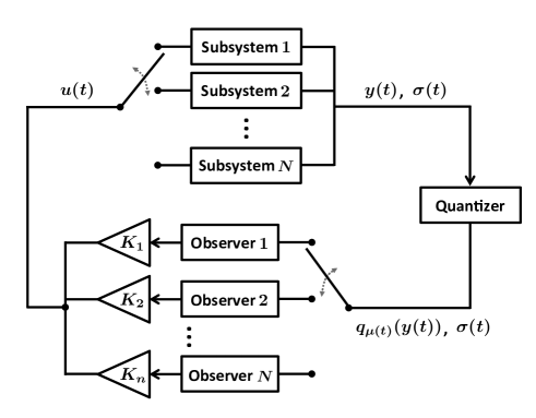
Figure 1: Continuous-time switched system with quantized output feedback.

Theorem II.4

Define $\Theta$ by

$$\Theta:=\frac{2\max_{p\in\mathcal{P}}\|P_{p}\hat{L}_{p}\|}{\underline{\lambda}_{Q}},\text{~{}~{}where~{}~{}}\hat{L}_{p}:=\begin{bmatrix}0\\ L_{p}\end{bmatrix}.$$ (17)

and let $M$ be large enough to satisfy

$$M>\max\left\{2\Delta,\quad\sqrt{\frac{\overline{\lambda}_{P}}{\underline{\lambda}_{P}}}\Theta\Delta C_{\max}\right\}.$$ (18)

If the average dwell time $\tau_{a}$ in (3) is larger than a certain value, then there exists a right-continuous and piecewise-constant function $\mu$ such that the closed-loop system (12) has the following two properties for every $x(0)\in\mathbb{R}^{\sf{n}}$ and every $\sigma(0)\in\mathcal{P}$:

(i) Convergence to the origin:  $\lim_{t\to\infty}z(t)=0$.

(ii) Lyapunov stability:  To every $\varepsilon>0$, there corresponds $\delta>0$ such that

$$|x(0)|<\delta\quad\Rightarrow\quad|z(t)|<\varepsilon~{}~{}~{}(t\geq 0).$$

We shall prove convergence to the origin and Lyapunov stability in Sections III and IV, respectively. We also present an update rule of the “zoom” parameter $\mu$ in Section 3. The sufficient condition on $\tau_{a}$ is given by (42) in Theorem III.6 below.

III The proof of convergence to the origin

Define $\Gamma$ and $\Lambda$ by

$$\Gamma:=\max_{p\in\mathcal{P}}\|A_{p}\|,\quad\Lambda:=\max\left\{1,~{}\max_{p,q\in\mathcal{P},p\not=q}\|R_{p,q}\|\right\}.$$

We split the proof into two stages: the “zooming-out” and “zooming-in” stages.

III-A Capturing the state of the closed-loop system by “zooming out”

Since the initial state $x(0)$ is unknown to the quantizer, we have to capture the state $z$ of the closed-loop system by “zooming out”, i.e., increasing the “zoom” parameter $\mu$. We first see that $z$ can be captured if we have a time-interval with a given length that has no switches.

Theorem III.1

Consider the closed-loop system (12). Set the control input $u=0$. Choose $\tau>0$, and define $\Upsilon_{p}(\tau):=\max_{0\leq t\leq\tau}\left\|C_{p}e^{A_{p}t}\right\|$ and the observability Gramian

$$W_{p}(\tau):=\int^{\tau}_{0}e^{A_{p}^{\top}t}C_{p}^{\top}C_{p}e^{A_{p}t}dt.$$

Assume that there exists $s_{0}\geq 0$ such that we can observe

$$|q_{\mu(t)}(y(t))|\leq M\mu(t)-\Delta\mu(t)$$ (19)

$$\sigma(t)=\sigma(s_{0})=:p$$ (20)

for all $t\in[s_{0},s_{0}+\tau)$. Let the “zoom” parameter $\mu$ be piecewise continuous and monotone increasing in $[0,s_{0}+\tau)$. If we set the state estimate $\xi$ at $t=s_{0}+\tau$ by

$$\xi(s_{0}+\tau):=e^{A_{p}\tau}\left(W_{p}(\tau)^{-1}\int^{\tau}_{0}e^{A_{p}^{\top}t}C_{p}^{\top}q_{\mu(s_{0}+t)}(y(s_{0}+t))dt\right)$$ (21)

and if we choose $\mu(s_{0}+\tau)$ so that

$$\mu(s_{0}+\tau)\geq\sqrt{\frac{\overline{\lambda}_{p}}{\underline{\lambda}_{p}}}\frac{C_{\max}}{M}\biggl{(}|\xi(s_{0}+\tau)|+2\|W_{p}(\tau)^{-1}\|\tau\Upsilon_{p}(\tau)\left\|e^{A_{p}\tau}\right\|\Delta\mu((s_{0}+\tau)^{-})\biggr{)},$$ (22)

then $z(s_{0}+\tau)\in\mathscr{R}_{1}(\mu(s_{0}+\tau),\sigma(s_{0}+\tau))$.

Proof: Since no switch occurs by (20), we can easily obtain this result by extending Theorem 5 in [13] for the non-switched case. We therefore omit the proof; see also the conference version [19]. $\Box$

It follows from Theorem III.1 that in order to capture the state $z$, it is enough to show the existence of $s_{0}\geq 0$ satisfying (19) and (20) for all $t\in[s_{0},s_{0}+\tau)$. To this end, we use the following lemma on average dwell time $\tau_{a}$:

Lemma III.2

Fix an initial time $t_{0}\geq 0$. Suppose that $\sigma$ satisfies the average dwell-time assumption (3). Let $\tau\in(0,\tau_{a})$. If we choose $N\in\mathbb{N}$ so that

$$N>\frac{\tau_{a}}{\tau_{a}-\tau}\left(N_{0}-\frac{\tau}{\tau_{a}}\right),$$ (23)

then there exists $\upsilon\in[0,(N-1)\tau]$ such that $N_{\sigma}(t_{0}+\upsilon+\tau,t_{0}+\upsilon)=0$.

Proof: Let us denote the switching times by $t_{1},t_{2},\dots$, and fix $N\in\mathbb{N}$. Suppose that

$$N_{\sigma}(t_{0}+\upsilon+\tau,t_{0}+\upsilon)>0$$ (24)

for all $\upsilon\in[0,(N-1)\tau]$. Then we have

$$t_{k}-t_{k-1}\leq\tau\qquad(k=1,\dots,N).$$ (25)

Indeed, if $t_{k}-t_{k-1}>\tau$ for some $k\leq N$ and if we let $\bar{k}$ be the smallest such integer, then we obtain

$$t_{\bar{k}-1}-t_{0}\leq(\bar{k}-1)\tau\leq(N-1)\tau$$

and $N_{\sigma}(t_{\bar{k}-1}+\tau,t_{\bar{k}-1})=0$. This contradicts (24) with $\upsilon=t_{\bar{k}-1}-t_{0}\in[0,(N-1)\tau]$. Thus we have (25).

From (25), we see that for $0<\epsilon<t_{1}$,

$$t_{N}-(t_{1}-\epsilon)=\sum_{k=2}^{N}(t_{k}-t_{k-1})+\epsilon\leq(N-1)\tau+\epsilon$$

It follows from (3) that

$$N=N_{\sigma}(t_{N},t_{1}-\epsilon) \leq N_{0}+\frac{(N-1)\tau+\epsilon}{\tau_{a}}.$$

Therefore $N$ satisfies the following inequality:

$$N\leq\frac{\tau_{a}}{\tau_{a}-\tau}\left(N_{0}-\frac{\tau-\epsilon}{\tau_{a}}\right).$$ (26)

Since $\epsilon\in(0,t_{1})$ was arbitrary, (26) is equivalent to

$$N\leq\frac{\tau_{a}}{\tau_{a}-\tau}\left(N_{0}-\frac{\tau}{\tau_{a}}\right).$$ (27)

Thus we have shown that if (24) holds for all $\upsilon\in[0,(N-1)\tau]$, then $N\in\mathbb{N}$ satisfies (27). The contraposition of this statement gives a desired result. $\Box$

Theorem III.3

Consider the closed-loop system (12) with average dwell-time property (3). Set the control input $u=0$. Fix $\chi>0$, $\bar{\tau}>0$, and $\tau\in(0,\tau_{a})$. Increase $\mu$ in the following way: $\mu(t)=1$ for $t\in[0,\bar{\tau})$,

$$\mu(t)=\Lambda^{N_{0}}\cdot\left(\Lambda^{1/\tau_{a}}e^{\Gamma}\right)^{(1+\chi)k\bar{\tau}}$$ (28)

for $t\in[k\bar{\tau},(k+1)\bar{\tau})$ and $k\in\mathbb{N}$. Then there exists $s_{0}\geq 0$ such that (19) and (20) hold for all $t\in[s_{0},s_{0}+\tau)$.

Proof: If $n$ switches occur in the interval $(0,t]$, then we have

$$|x(t)|\leq\left(\prod_{k=1}^{n}\Lambda\right)\cdot e^{\Gamma t}\cdot|x(0)|.$$

Since $\Lambda\geq 1$, it follows from (3) that

$$|x(t)|\leq\Lambda^{\left(N_{0}+\frac{t}{\tau_{a}}\right)}\cdot e^{\Gamma t}\cdot|x(0)|.$$ (29)

Clearly, this inequality holds in the case when no switches occur. Since (18) shows that $M-2\Delta>0$ and since the growth rate of $\mu(t)$ is larger than that of $|y(t)|$, there exists $s_{0}^{\prime}\geq 0$ such that

$$\left|y(t)\right|\leq M\mu(t)-2\Delta\mu(t)\qquad(t\geq s_{0}^{\prime}).$$ (30)

In conjunction with (4), this implies that (19) holds for every $t\geq s_{0}^{\prime}$. Let $N$ be an integer satisfying (23). Then Lemma III.2 guarantees the existence of $s_{0}\in[s_{0}^{\prime},s_{0}^{\prime}+(N-1)\tau]$ such that (20) holds for every $t\in[s_{0},s_{0}+\tau)$. This completes the proof. $\Box$

It follows from Theorems III.1 and III.3 that if we update the “zoom” parameter $\mu$ as in (28) and if we set the state estimate $\xi$ by (21), then the state $z$ of the closed-loop system can be captured.

Remark III.4

If the initial state $x(0)$ is sufficiently small, then $s_{0}^{\prime}$ in (30) is zero. In this situation, we can capture $z$ by $t=N\tau$ for all switching signal with average dwell-time property (3). We use this fact for the proof of Lyapunov stability; see Section 4.

III-B Measuring the output by “zooming in”

Next we drive the state $z$ of the closed-loop system to the origin by “zooming-in”, i.e., decreasing the “zoom” parameter $\mu$. Since $\mu$ increases at each switching time during this stage, the term “zooming-in stage” may be misleading. However, $\mu$ decreases overall under a certain average dwell-time assumption (3), so we use the term “zooming-in” as in [12, 13].

Let us first consider a fixed “zoom” parameter $\mu$. The following lemma shows that if no switches occur, then the state trajectories move from a large level set to a small level set of the Lyapunov function $V_{p}(z):=z^{\top}P_{p}z$ in a finite time that is independent of the mode $p$:

Lemma III.5

Define $F_{p}$ and $\hat{L}_{p}$ as in (11) and (17), respectively. Fix $p\in\mathcal{P}$, and consider the non-switched system

$$\dot{z}=F_{p}z+\hat{L}_{p}(q_{\mu}(y)-y).$$ (31)

Choose $\kappa>0$. If $M$ satisfies

$$\sqrt{\underline{\lambda}_{P}}M>\sqrt{\overline{\lambda}_{P}}\Theta\Delta(1+\kappa)C_{\max},$$ (32)

where $\overline{\lambda}_{P}$, $\underline{\lambda}_{P}$ $C_{\max}$, and $\Theta$ are defined by (16) and (17), then the following two level sets of the Lyapunov function $V_{p}(z):=z^{\top}P_{p}z$ are invariant regions for every trajectory of (31):

$$\mathscr{R}_{1}(\mu,p) :=\left\{z\in\mathbb{R}^{\sf n}:V_{p}(z)\leq\frac{\underline{\lambda}_{P}M^{2}\mu^{2}}{C_{\max}^{2}}\right\}$$ (33)

$$\mathscr{R}_{2}(\mu,p) :=\left\{z\in\mathbb{R}^{\sf n}:V_{p}(z)\leq\overline{\lambda}_{P}(\Theta\Delta(1+\kappa))^{2}\mu^{2}\right\}.$$ (34)

Furthermore, if $z(t)\in\mathscr{R}_{1}(\mu,p)\setminus\mathscr{R}_{2}(\mu,p)$ for all $t\in[t_{1},t_{2}]$, then

$$V_{p}(z(t_{2}))\leq V_{p}(z(t_{1}))-(t_{2}-t_{1})\underline{\lambda}_{Q}\kappa(1+\kappa)(\Theta\Delta\mu)^{2}$$ (35)

for every $p\in\mathcal{P}$. Hence if $T$ satisfies

$$T>\frac{\underline{\lambda}_{P}M^{2}-\overline{\lambda}_{P}(\Theta\Delta(1+\kappa)C_{\max})^{2}}{\underline{\lambda}_{Q}\kappa(1+\kappa)(\Theta\Delta C_{\max})^{2}},$$ (36)

then every trajectory of (31) with an initial state $z(0)\in\mathscr{R}_{1}(\mu,p)$ satisfies $z(T)\in\mathscr{R}_{2}(\mu,p)$．

Proof: Since the mode $p\in\mathcal{P}$ is fixed, this lemma is a trivial extension of Lemma 5 in [13] for single-modal systems. We therefore omit its proof; see also the conference version [19]. $\Box$

Using Lemma III.5, we obtain an update rule of the “zoom” parameter $\mu$ to drive the state $z$ to the origin.

Theorem III.6

Consider the system (31) under the same assumptions as in Lemma III.5. Assume that $z(t_{0})\in\mathscr{R}_{1}(\mu(t_{0}),\sigma(t_{0}))$. For each $p_{1},p_{2}\in\mathcal{P}$ with $p_{1}\not=p_{2}$, the positive definite matrices $P_{p_{1}}$ and $P_{p_{2}}$ in the Lyapunov equation (13) satisfy

$$z^{\top}J_{p_{2},p_{1}}^{\top}P_{p_{2}}J_{p_{2},p_{1}}z\leq c_{p_{2},p_{1}}\cdot z^{\top}P_{p_{1}}z\qquad(z\in\mathbb{R}^{2{\sf n}})$$ (37)

for some $c_{p_{2},p_{1}}>0$. Define $c$ and $\Omega$ by

$$c:=\max\left\{1,~{}\max_{p_{1},p_{2}\in\mathcal{P},p_{1}\not=p_{2}}c_{p_{2},p_{1}}\right\}$$ (38)

$$\Omega:=\sqrt{\frac{\overline{\lambda}_{P}}{\underline{\lambda}_{P}}}\frac{\Theta\Delta(1+\kappa)C_{\max}}{M}<1.$$ (39)

Fix $T>0$ so that (36) is satisfied, and set the “zoom” parameter $\mu(t_{0}+kT+t)$ for all $k\in\mathbb{Z}$ and $t\in(0,T]$ in the following way: If no switches occur in the interval $(t_{0}+kT,t_{0}+(k+1)T]$, then

$$\mu(t_{0}+kT+t)=\begin{cases}\mu(t_{0}+kT)&(0<t<T)\\ \Omega\mu(t_{0})&(t=T);\end{cases}$$ (40)

otherwise,

$$\mu(t_{0}+kT+t)=\begin{cases}\mu(t_{0}+kT)&(0<t<t_{1})\\ \sqrt{\prod_{\ell=0}^{i-1}c_{\sigma(t_{\ell+1}),\sigma(t_{\ell})}}\cdot\mu(t_{0})&(t_{i}\leq t<t_{i+1},~{}i=1,\dots,n)\\ \Omega\prod_{\ell=0}^{n-1}c_{\sigma(t_{\ell+1}),\sigma(t_{\ell})}\cdot\mu(t_{0})&(t=T),\end{cases}$$ (41)

where $t_{1},\dots,t_{n}$ are the switching times in the interval $(t_{0}+kT,t_{0}+(k+1)T]$. Then $z(t)\in\mathscr{R}_{1}(\mu(t),\sigma(t))$ for all $t\geq t_{0}$. Furthermore, if $\tau_{a}$ satisfies

$$\tau_{a}>\frac{\log(c)}{2\log(1/\Omega)}T,$$ (42)

then $\lim_{t\to\infty}z(t)=0$.

Proof: To prove that $z(t)\in\mathscr{R}_{1}(\mu(t),\sigma(t))$ for all $t\geq t_{0}$, it is enough to show that if $z(t_{0})\in\mathscr{R}_{1}(\mu(t_{0}),\sigma(t_{0}))$, then

$$z(t)\in\mathscr{R}_{1}(\mu(t),\sigma(t))\qquad(t_{0}\leq t\leq t_{0}+T)$$ (43)

Let us first investigate the case without switching on the interval $(t_{0},t_{0}+T]$. We see from Lemma III.5 that $z(t)\in\mathscr{R}_{1}(\mu(t),\sigma(t))$ for all $t\in[t_{0},t_{0}+T)$ and that $z((t_{0}+T)^{-})\in\mathscr{R}_{2}(\mu(t_{0}),\sigma(t_{0}))$. Since $\mu(t_{0}+T)=\Omega\mu(t_{0})$, a routine calculation shows that $z(t_{0}+T)\in\mathscr{R}_{1}(\mu(t_{0}+T),\sigma(t_{0}+T))$.

We now study the switched case. Let $t_{1},t_{2},\dots,t_{n}$ be the switching times in the interval $(t_{0},t_{0}+T]$. Let us define $t_{n+1}:=t_{0}+T$ for simplicity of notation. Lemma III.5 implies that $\mathscr{R}_{i}(\mu(t_{k}),\sigma(t_{k}))$ ($i=1,2$) are invariant sets for all $t\in[t_{k},t_{k+1})$, $k=0,\dots,n$. Moreover, by (37), if $z(t_{k}^{-})\in\mathscr{R}_{i}(\mu(t_{k}^{-}),\sigma(t_{k}^{-}))$, then $z(t_{k})\in\mathscr{R}_{i}(\mu(t_{k}),\sigma(t_{k}))$ ($i=1,2$) for all $k=1,\dots,n$. Hence $z(t_{0})\in\mathscr{R}_{1}(\mu(t_{0}),\sigma(t_{0}))$ leads to

$$z(t)\in\mathscr{R}_{1}(\mu(t),\sigma(t))\qquad(t_{0}\leq t<t_{n+1}).$$ (44)

To obtain

$$z(t_{n+1})\in\mathscr{R}_{1}(\mu(t_{n+1}),\sigma(t_{n+1})),$$ (45)

we show that $z(t_{n+1}^{-})\in\mathscr{R}_{2}(\mu(t_{n+1}^{-}),\sigma(t_{n+1}^{-}))$. Assume, to reach a contradiction, that

$$z(t_{n+1}^{-})\not\in\mathscr{R}_{2}(\mu(t_{n+1}^{-}),\sigma(t_{n+1}^{-})).$$ (46)

Since $\mathscr{R}_{2}(\mu(t),\sigma(t))$ is an invariant region for all $t\in[t_{0},t_{n+1})$, we also have

$$z(t)\not\in\mathscr{R}_{2}(\mu(t),\sigma(t))\qquad(t_{0}\leq t<t_{n+1}).$$

Define a Lyapunov function $V_{p}(z):=z^{\top}P_{p}z$ for each $p\in\mathcal{P}$. Since a Filippov solution is (absolutely) continuous, $\lim_{t\nearrow t_{k}}V_{\sigma(t)}(z(t))$ exists for each $k=1,\dots,n+1$. From (46), we obtain

$$\lim_{t\nearrow t_{n+1}}V_{\sigma(t)}(z(t))\geq\overline{\lambda}_{P}(\Theta\Delta(1+\kappa))^{2}\mu(t_{n})^{2}.$$ (47)

On the other hand, since $z(t)\in\mathscr{R}_{1}(\mu(t),\sigma(t))\setminus\mathscr{R}_{2}(\mu(t),\sigma(t))$ for all $t\in[t_{0},t_{1}]$, (35) gives

$$\lim_{t\nearrow t_{1}}V_{\sigma(t)}(z(t))\!\leq\!\left(\frac{\underline{\lambda}_{P}M^{2}}{C_{\max}^{2}}\!-\!(t_{1}\!-\!t_{0})\underline{\lambda}_{Q}\kappa(1\!+\!\kappa)(\Theta\Delta)^{2}\right)\mu(t_{0})^{2},$$

and hence we have from $\mu(t_{1})=\sqrt{c_{\sigma(t_{1}),\sigma(t_{0})}}\mu(t_{0})$ that

$$V_{\sigma(t_{1})}(z(t_{1})) =z(t_{1}^{-})^{\top}J_{\sigma(t_{1}),\sigma(t_{1}^{-})}^{\top}P_{\sigma({t_{1}})}J_{\sigma(t_{1}),\sigma(t_{1}^{-})}z(t_{1}^{-})$$

$$\leq c_{\sigma(t_{1}),\sigma(t_{0})}\cdot\left(\lim_{t\nearrow t_{1}}V_{\sigma(t)}(z(t))\right)$$

$$=\left(\frac{\underline{\lambda}_{P}M^{2}}{C_{\max}^{2}}\!-\!(t_{1}\!-\!t_{0})\underline{\lambda}_{Q}\kappa(1\!+\!\kappa)(\Theta\Delta)^{2}\right)\!\mu(t_{1})^{2}.$$

If we repeat this process and use (36), then

$$\lim_{t\nearrow t_{n+1}}V_{\sigma(t)}(z(t)) \leq\left(\frac{\underline{\lambda}_{P}M^{2}}{C_{\max}^{2}}-T\underline{\lambda}_{Q}\kappa(1+\kappa)(\Theta\Delta)^{2}\right)\mu(t_{n})^{2}$$

$$<\overline{\lambda}_{P}(\Theta\Delta(1+\kappa))^{2}\mu(t_{n})^{2},$$ (48)

which contradicts (47). Thus we obtain

$$z(t_{n+1}^{-})\in\mathscr{R}_{2}(\mu(t_{n+1}^{-}),\sigma(t_{n+1}^{-})),$$

and hence (45) holds.

From (44) and (45), we derive the desired result (43), because $t_{n+1}=t_{0}+T$.

Finally, since $c\geq 1$, (3) gives

$$\mu(t_{0}+mT+t)\leq\Omega^{m}\sqrt{c^{N_{\sigma}(t_{0}+mT+t,t_{0})}}\mu(t_{0})\leq\sqrt{c^{N_{0}+T/\tau_{a}}}\cdot\left(\Omega\sqrt{c^{T/\tau_{a}}}\right)^{m}\mu(t_{0})$$ (49)

for every $m\geq 0$ and $t\in[0,T)$. If $\Omega\sqrt{c^{T/\tau_{a}}}<1$, that is, if the average dwell time $\tau_{a}$ satisfies (42), then $\lim_{t\to\infty}\mu(t)=0$. Since $z(t)\in\mathscr{R}_{1}(\mu(t),\sigma(t))$ for all $t\geq t_{0}$, we obtain $\lim_{t\to\infty}z(t)=0$. $\Box$

Remark III.7

(a)  We can compute $c_{p_{2},p_{1}}$ by linear matrix inequalities. Moreover, if the jump matrix $R_{p_{2},p_{1}}$ in (2) is invertible, then Lemma 13 of [22] gives an explicit formula for $c_{p_{2},p_{1}}$.

(b)  The proposed method is sensitive to the time-delay of the switching signal at the “zooming-in” stage. If the switching signal is delayed, a mode mismatch occurs between the plant and the controller. Here we do not proceed along this line to avoid technical issues. See also [23] for the stabilization of asynchronous switched systems with time-delays.

(c)  We have updated the “zoom” parameter $\mu$ at each switching time in the “zooming-in” stage. If we would not, switching could lead to instability of the closed-loop system. In fact, since the state $z$ may not belong to the invariant region $\mathscr{R}_{1}(\mu,\sigma)$ without adjusting $\mu$, the quantizer may saturate.

(d)  Similarly, “pre-emptively” multiplying $\mu$ at time $T_{0}+kT$ by $c^{n}$ does not work, either. This is because such an adjustment does not make $\mathscr{R}_{1}(\mu,\sigma)$ invariant for the state trajectories. For example, consider the situation where the state $z$ belongs to $\mathscr{R}_{2}(\mu,\sigma)$ at $t=T_{0}+kT$ due to this pre-emptively adjustment. Then $z$ does not converge to the origin. Let $t_{1}>T_{0}+kT$ be a switching time. Since $\mathscr{R}_{2}(\mu(t_{1}^{-}),\sigma(t_{1}^{-}))$ may not be a subset of $\mathscr{R}_{1}(\mu(t_{1}),\sigma(t_{1}))$, it follows that $z$ does not belong to the invariant region $\mathscr{R}_{1}(\mu,\sigma)$ at $t=t_{1}$ in general.

IV The proof of Lyapunov stability

Let us denote by $\mathscr{B}_{\varepsilon}$ the open ball with center at the origin and radius $\varepsilon$ in $\mathbb{R}^{2{\sf n}\times 2{\sf n}}$. In what follows, we use the same letters as in the previous section and assume that the average dwell time $\tau_{a}$ satisfies (42).

The proof consists of three steps:

1. Obtain an upper bound of the time $t_{0}$ at which the quantization process transitions from the “zoom-out” stage to the “zoom-in” stage.

2. Show that there exists a time $t_{\varepsilon}\geq t_{0}$ such that the state $z$ satisfies $|z(t)|<\varepsilon$ for all $t\geq t_{\varepsilon}$.

3. Set $\delta>0$ so that if $|x(0)|<\delta$, then $|z(t)|<\varepsilon$ for all $t<t_{\varepsilon}$.

We break the proof of Lyapunov stability into the above three steps.

1) Let $N\in\mathbb{N}$ satisfy (24) and let $\delta>0$ be small enough to satisfy

$$C_{\max}\cdot\Lambda^{N_{0}}\left(\Lambda^{1/\tau_{a}}e^{\Gamma}\right)^{N\tau}\delta<\Delta_{0}.$$ (50)

We see from the state bound (29) that $q_{\mu(t)}(y(t))=0$ for $t\in[0,N\tau]$ from Assumption II.2. As we mentioned in Remark III.4 briefly, Lemma III.2 implies that the time $t_{0}$, at which the stage changes from “zooming-out” to “zooming-in”, satisfies $t_{0}\leq N\tau$ for every switching signal with the average dwell-time assumption (3).

2) Fix $\alpha>0$. By (21), $\xi(t_{0})=0$, and hence we see from (22) that $\mu(t_{0})$ achieving $z(t_{0})\in\mathscr{R}_{1}(\mu(t_{0}),\sigma(t_{0}))$ can be chosen so that

$$\alpha\leq\mu(t_{0})\leq\bar{\mu},$$ (51)

where $\bar{\mu}$ is defined by

$$\bar{\mu}:=\max\Biggl{\{}\alpha,~{}~{}2\sqrt{\frac{\overline{\lambda}_{P}}{\underline{\lambda}_{P}}}\frac{\Delta\tau C_{\max}\Lambda^{N_{0}}\left(\Lambda^{1/\tau_{a}}e^{\Gamma}\right)^{(1+\chi)N\tau}}{M}\cdot\max_{p\in\mathcal{P}}\left(\|W_{p}(\tau)^{-1}\|\Upsilon_{p}(\tau)\left\|e^{A_{p}\tau}\right\|\right)\Biggr{\}}.$$

Note that $\bar{\mu}$ is independent of switching signals.

Let $\bar{m}>0$ be the smallest integer satisfying

$$\bar{m}>\frac{\log(\bar{\mu}M\sqrt{c^{N_{0}+T/\tau_{a}}}/(\varepsilon C_{\max}))}{\log(1/(\Omega\sqrt{c^{T/\tau_{a}}}))}.$$ (52)

Define $t_{\varepsilon}:=t_{0}+\bar{m}T$. Since $c\geq 1$ and $\Omega\sqrt{c^{T/\tau_{a}}}<1$, (40) and (41) give

$$\mu(t_{\varepsilon}+kT+t) =\mu(t_{0}+(\bar{m}+k)T+t))$$

$$\leq\sqrt{c^{N_{0}+T/\tau_{a}}}\cdot\left(\Omega\sqrt{c^{T/\tau_{a}}}\right)^{\bar{m}+k}\mu(t_{0})$$

$$\leq\sqrt{c^{N_{0}+T/\tau_{a}}}\cdot\left(\Omega\sqrt{c^{T/\tau_{a}}}\right)^{\bar{m}}\bar{\mu}$$

for all $k\geq 0$ and $t\in[0,T)$. Since $\bar{m}$ satisfies (52), it follows that that $\mathscr{R}_{1}(\mu(t),\sigma(t))$ lies in $\mathscr{B}_{\varepsilon}$ for all $t\geq t_{\varepsilon}$. Recall that $z(t_{0})\in\mathscr{R}_{1}(\mu(t_{0}),\sigma(t_{0}))$ and that $\mathscr{R}_{1}(\mu(t),\sigma(t))$ is an invariant region for all $t\geq t_{0}$ from Theorem III.6. Thus we have

$$|z(t)|<\varepsilon\qquad(t\geq t_{\varepsilon}).$$ (53)

3) Define $\underline{c}:=\min\{1,\min_{p_{1},p_{2}\in\mathcal{P},p_{1}\not=p_{2}}c_{p_{2},p_{1}}\}.$ Since $\underline{c}\leq 1$, it follows from (40) (41), and (51) that

$$\mu(t)\geq\Omega^{\bar{m}}\sqrt{\underline{c}^{N_{0}+\bar{m}T/\tau_{a}}}\mu(t_{0})\geq\alpha\Omega^{\bar{m}}\sqrt{\underline{c}^{N_{0}+\bar{m}T/\tau_{a}}}=:\eta.$$ (54)

for all $t\in[t_{0},t_{\varepsilon}]$. Set $\delta>0$ so that

$$C_{\max}\cdot\Lambda^{N_{0}}\left(\Lambda^{1/\tau_{a}}e^{\Gamma}\right)^{N\tau+\bar{m}T}\delta<\eta\Delta_{0}$$ (55)

$$\Lambda^{N_{0}}\left(\Lambda^{1/\tau_{a}}e^{\Gamma}\right)^{N\tau+\bar{m}T}\delta<\varepsilon/2.$$ (56)

Since $t_{\varepsilon}=t_{0}+\bar{m}T\leq N\tau+\bar{m}T$, by (29), (50), (54), and (55), Assumption II.2 gives $q_{\mu(t)}(y(t))=0$ in the interval $[0,t_{\varepsilon}]$, so $\xi(t)=0$ and $u(t)=0$ in the same interval. Combining this with (56), we obtain $|x(t)|\leq\Lambda^{N_{0}}\left(\Lambda^{1/\tau_{a}}e^{\Gamma}\right)^{(N\tau+\bar{m}T)}\delta<\varepsilon/2$ for all $t<t_{\varepsilon}$. Thus

$$|z(t)|=2|x(t)|<\varepsilon\qquad(t<t_{\varepsilon}).$$ (57)

From (53) and (57), we see that Lyapunov stability can be achieved. $\Box$

V Numerical examples

Consider the continuous-time switched system (10) with the following two modes:

$$(A_{1},B_{1},C_{1}) =\left(\begin{bmatrix}1&-0.3\\ 0.4&-4\end{bmatrix},\ \begin{bmatrix}1\\ 0\end{bmatrix},\ \begin{bmatrix}1&1\end{bmatrix}\right)$$

$$(A_{2},B_{2},C_{2}) =\left(\begin{bmatrix}-0.1&1\\ -1&0.1\end{bmatrix},\ \begin{bmatrix}0\\ 1\end{bmatrix},\ \begin{bmatrix}0&-1\end{bmatrix}\right)$$

with jump matrices $R_{1,2}=R_{2,1}=I$. As the feedback gain and the observer gain of each mode, we take

$$(K_{1},L_{1}) =\left(\begin{bmatrix}-3&-2\end{bmatrix},~{}\begin{bmatrix}-4\\ 0\end{bmatrix}\right)$$

$$(K_{2},L_{2}) =\left(\begin{bmatrix}0&1\end{bmatrix},~{}L_{2}=\begin{bmatrix}0\\ -1\end{bmatrix}\right).$$

Let $q$ be a uniform-type quantizer with parameters $M=10$, $\Delta=0.05.$ The parameters $\tau,\bar{\tau},\chi$ in the “zooming-out” stage are $\tau=0.5$, $\bar{\tau}=1$, and $\chi=0.1$. Also, define $Q_{1}$ and $Q_{2}$ in (13) and $\kappa$ in (32) by $Q_{1}:=\mathop{\rm diag}\nolimits(6,6,2,6)$, $Q_{2}:=\mathop{\rm diag}\nolimits(1,1,1,1),$ $\kappa:=4.5$, where $\mathop{\rm diag}\nolimits(e_{1},\dots,e_{4})$ means a diagonal matrix whose diagonal elements starting in the upper left corner are $e_{1},\dots,e_{4}$. Then we obtain $T=0.6025$ in (36), $\Omega=0.9063$ in (39), $c=1.9867$ in (38), and $\tau_{a}=2.0744$ in (42).

Figure 2 (a) and (b) show that the Euclidean norm of the state $x$ and the estimate $\xi$, and the “zoom” parameter $\mu$, respectively, with initial condition $x(0)=[5~{}-\!10]^{\top}$ and $\mu(0)=1$. The vertical dashed-dotted line indicates the switching times $t=3.5,7,20$. In this example, the “zooming-out” stage finished at $t=0.5$. We see the non-smoothness of $x,\xi$ and the increase of $\mu$ at the switching times $t=3.5,7,20$ because of switches and quantizer updates. Not surprisingly, the adjustments of $\mu$ in (22) and (41) are conservative.

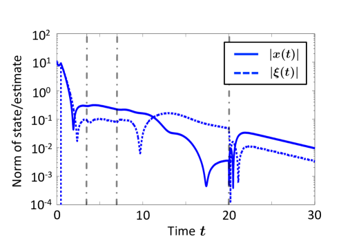
(a) Norms of state $x$ and estimate $\xi$.

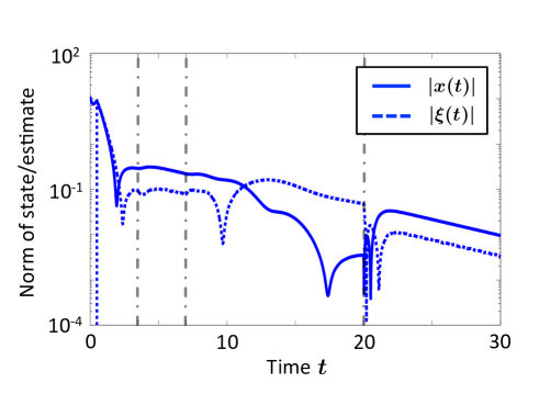
(b) Zoom parameter $\mu$.

Figure 2: Simulation with initial condition $x(0)=[5~{}-\!10]^{\top}$ and $\sigma(0)=1$. The vertical dashed-dotted line indicates the switching times $t=3.5,7,20$.

VI Concluding remarks

We have proposed an update rule of dynamic quantizers to stabilize continuous-time switched systems with quantized output feedback. The average dwell-time property has been utilized for the state reconstruction in the “zooming-out” stage and for convergence to the origin in the “zooming-in” stage. The update rule not only periodically decreases the “zoom” parameter to drive the state to the origin, but also adjusts the parameter at each switching time to avoid quantizer saturation. Future work involves designing the controller and the quantizer simultaneously, and addressing more general systems by incorporating disturbances and nonlinear dynamics.

References

• [1] G. N. Nair, F. Fagnani, S. Zampieri, and R. J. Evans, “Feedback control under data rate constraints: An overview,” Proc. IEEE, vol. 95, pp. 108–137, 2007.
• [2] H. Ishii and K. Tsumura, “Data rate limitations in feedback control over network,” IEICE Trans. Fundamentals, vol. E95-A, pp. 680–690, 2012.
• [3] G. S. Deaecto, J. C. Geromel, F. S. Garcia, and J. A. Pomilio, “Switched affine systems control design with application to DC–DC converters,” IET Control Theory Appl., vol. 4, pp. 1201–1210, 2010.
• [4] M. Rinehart, M. Dahleh, D. Reed, and I. Kolmanovsky, “Suboptimal control of switched systems with an application to the DISC engine,” IEEE Trans. Control Systems Tech., vol. 16, pp. 189–201, 2008.
• [5] R. Shorten, F. Wirth, O. Mason, K. Wulff, and C. King, “Stability criteria for switched and hybrid systems,” SIAM Review, vol. 49, pp. 545–592, 2007.
• [6] H. Lin and P. J. Antsaklis, “Stability and stabilizability of switched linear systems: a survey of recent results,” IEEE Trans. Automat. Control, vol. 54, pp. 308–322, 2009.
• [7] D. Liberzon, Switching in Systems and Control.   Birkhäuser, Boston, 2003.
• [8] G. N. Nair, S. Dey, and R. J. Evans, “Infinmum data rates for stabilising Markov jump linear systems,” in Proc. 42nd IEEE CDC, 2003.
• [9] N. Xiao, L. Xie, and M. Fu, “Stabilization of Markov jump linear systems using quantized state feedback,” Automatica, vol. 46, pp. 1696–1702, 2010.
• [10] Q. Xu, C. Zhang, and G. E. Dullerud, “Stabilization of Markovian jump linear systems with log-quantized feedback,” J. Dynamic Systems, Meas, Control, vol. 136, pp. 1–10 (031 919), 2013.
• [11] M. Wakaiki and Y. Yamamoto, “Quantized feedback stabilization of sampled-data switched linear systems,” in Proc. 19th IFAC WC, 2014.
• [12] R. W. Brockett and D. Liberzon, “Quantized feedback stabilization of linear systems,” IEEE Trans. Automat. Control, vol. 45, pp. 1279–1289, 2000.
• [13] D. Liberzon, “Hybrid feedback stabilization of systems with quantized signals,” Automatica, vol. 39, pp. 1543–1554, 2003.
• [14] J. P. Hespanha and A. S. Morse, “Stability of switched systems with average dwell-time,” in Proc. 38th IEEE CDC, 1999.
• [15] D. Liberzon, “Finite data-rate feedback stabilization of switched and hybrid linear systems,” Automatica, vol. 50, pp. 409–420, 2014.
• [16] M. Wakaiki and Y. Yamamoto, “Output feedback stabilization of switched linear systems with limited information,” in Proc. 53rd IEEE CDC, 2014.
• [17] G. Yang and D. Liberzon, “Stabilizing a switched linear system with disturbance by sampled-data quantized feedback,” in Proc. ACC’15, 2015.
• [18] D. Liberzon, “On stabilization of linear systems with limited information,” IEEE Trans. Automat. Control, vol. 48, pp. 304–307, 2003.
• [19] M. Wakaiki and Y. Yamamoto, “Quantized output feedback stabilization of switched linear systems,” in Proc. MTNS’14, 2014.
• [20] D. Liberzon and D. Nešić, “Input-to-state stabilization of linear systems with quantized state measurement,” IEEE Trans. Automat. Control, vol. 52, pp. 767–781, 2007.
• [21] A. F. Filippov, Differential Equations with Discontinuous Righthand Sides.   Dordrecht: Kluwer, 1988.
• [22] A. Tanwani and D. Liberzon, “Robust invertibility of switched linear systems,” in Proc. 50th CDC, 2011.
• [23] D. Ma and J. Zhao, “Stabilization of networked switched linear systems: An asynchronous switching delay system approach,” Systems Control Lett., vol. 77, pp. 46–54, 2015.