A Sustainability Condition for Stochastic Forest Model

Abstract.

A stochastic forest model of young and old age class trees is studied. First, we prove existence, uniqueness and boundedness of global nonnegative solutions. Second, we investigate asymptotic behavior of solutions by giving a sufficient condition for sustainability of the forest. Under this condition, we show existence of a Borel invariant measure. Third, we present several sufficient conditions for decline of the forest. Finally, we give some numerical examples.

T$\hat{\text{o}}$n Vi$\hat{\d{e}}$t Tạ^†

Promotive Center for International Education and Research of Agriculture

Faculty of Agriculture, Kyushu University

6-10-1 Hakozaki, Nishi-ku, Fukuoka 812-8581, Japan

Linh Thi Hoai Nguyen

Department of Information and Physical Sciences

Graduate School of Information Science and Technology, Osaka University

1-5 Yamadaoka, Suita, Osaka 565-0871, Japan

Atsushi Yagi^‡

Department of Applied Physics, Graduate School of Engineering, Osaka University

1-5 Yamadaoka, Suita, Osaka 565-0871, Japan

1. Introduction

In 1975, Antonovsky [1] introduced a mono-species forest model with two age classes of trees:

$$\begin{cases}\frac{du}{dt}=\rho v-\gamma(v)u-fu,\\ \frac{dv}{dt}=fu-hv.\end{cases}$$ (1)

Here, $u$ and $v$ denote the tree densities of young and old age classes, respectively. The parameters $\rho,h$ and $f$ are a reproduction rate, mortality of old trees, and aging rate of young trees, respectively; while $\gamma(v)=a(v-b)^{2}+c$ is a mortality of young trees, which is allowed to depend on the old-tree density. In addition, $a,b,c,\rho,f$ and $h$ are assumed to be positive constants.

It is not difficult to see that for any pair $(u_{0},v_{0})$ of nonnegative initial values $u_{0}$ and $v_{0}$, the system (1) possesses a nonnegative and global solution. Furthermore, (1) possesses nonnegative stationary solutions given by

1. $O=(0,0)$

2. $P^{-}=\Big{(}\frac{h}{f}(b-\sqrt{\frac{\rho f-h(c+f)}{ah}}),b-\sqrt{\frac{\rho f-h(c+f)}{ah}}\Big{)}$                  (if $h\in[h_{*},h^{*}])$

3. $P^{+}=\Big{(}\frac{h}{f}(b+\sqrt{\frac{\rho f-h(c+f)}{ah}}),b+\sqrt{\frac{\rho f-h(c+f)}{ah}}\Big{)}$                  (if $h\in(0,h^{*}])$

where $h_{*}=\frac{\rho f}{ab^{2}+c+f},h^{*}=\frac{\rho f}{c+f}.$ The stability and instability of these solutions depends strongly on the magnitude of the mortality $h$ of old age class trees (see Table 1).

$h$	$(0,h_{*})$	$(h_{*},h^{*})$	$(h^{*},\infty)$
$O$	unstable	stable	glob. asymp. stable
$P^{+}$	stable	stable	$-$
$P^{-}$	$-$	unstable	$-$

Table 1. Stability and instability of stationary solutions of (1)

On the basis of (1), Kuznetsov et al. [11] introduced a mathematical model of mono-species forest with two age classes which takes into account the seed production and dispersion. The third author studied that model with his colleagues (see, e.g., [3, 4, 5, 15] and [17, Chapter 11]). It is shown that $h$ plays a crucial role in the asymptotic behavior of solutions.

In the real world, the parameters in the model may be random variables due to unpredictability resulting from environmental, ecological and biological disturbances. In principle, the deterministic forest model can not handle randomness. Investigating the role of fluctuation of parameters by using stochastic models should be an interesting problem in environmental and ecological sciences.

As mentioned above, the asymptotic behavior of solutions to the deterministic forest model depends strongly on the magnitude of $h$. Therefore, in this paper we restrict ourselves to consider a stochastic forest model, where $h$ is perturbed by (Gaussian) white noise. Since Gaussian white noises can be expressed as the generalized derivative of a Brownian motion, we make a substitution:

$$h\leadsto h-\sigma dw_{t}$$

in (1), where $\{w_{t},t\geq 0\}$ is a one-dimensional Brownian motion defined on a filtered complete probability space $(\Omega,\mathcal{F},\{\mathcal{F}_{t}\}_{t\geq 0},\mathbb{P})$, and $\sigma>0$ is the intensity of the white noise. Our stochastic forest model is then formulated by Itô stochastic differential equations in $\mathbb{R}^{2}$:

$$\begin{cases}du_{t}=\{\rho v_{t}-[a(v_{t}-b)^{2}+c+f]u_{t}\}dt,\\ dv_{t}=(fu_{t}-hv_{t})dt+\sigma v_{t}dw_{t}.\end{cases}$$ (2)

In this paper, we study the stochastic forest model (2). We prove existence of unique global solutions to (2) and then study their asymptotic behavior. On one hand, we present a sufficient condition for sustainability of the forest. Under this condition, we also prove existence of a non-trivial Borel invariant measure. On the other hand, we give several sufficient conditions for decline of the forest. The results are illustrated by a few numerical examples.

To prove existence of non-trivial invariant measures to (2), a common method is to find four one-dimensional processes, namely $u^{1},u^{2},v^{1}$ and $v^{2}$, which satisfy two conditions:

• $u_{t}$ and $v_{t}$ are bounded by these processes, i.e. $u^{1}(t)<u_{t}<u^{2}(t)$ and $v^{1}(t)<v_{t}<v^{2}(t)$ for $0<t<\infty$

• These four processes do not hit the boundaries in the sense that there exist $\epsilon>0$ and $M>0$ such that

  $$\begin{cases}\epsilon<u^{1}(t)<u^{2}(t)<M&\hskip 28.45274pt\text{a.s.},0<t<\infty,\\ \epsilon<v^{1}(t)<v^{2}(t)<M&\hskip 28.45274pt\text{a.s.},0<t<\infty\\ \end{cases}$$

However, this can not be done because

$$\liminf_{t\to\infty}v_{t}=0\hskip 28.45274pt\text{ a.s. (see Theorem \ref{T2})}.$$

To overcome this difficulty, we use the semigroup method presented in [6, 13]. First, we establish some estimates for the average of integrals of solutions (see (19) and (20)). Then, we construct a strongly continuous semigroup generated by solutions of (2). Using these estimates and a theorem in [13], we show that the semigroup enjoys an invariant measure.

The organization of the present paper is as follows. Section 2 proves existence and boundedness of unique global nonnegative solutions to (2). Section 3 investigates sustainability of the forest and existence of a Borel invariant measure. To the contrary, Section 4 presents some sufficient conditions for decline of the forest. Finally, Section 5 gives some numerical examples.

2. Global solutions

In this section, we prove existence of unique global nonnegative solutions to (2) and show boundedness of solutions.

Put $\mathbb{R}^{2}_{+}=\{(u,v);u>0,v>0\}.$ Denote by $\overline{\mathbb{R}^{2}_{+}}$ the closure of $\mathbb{R}^{2}_{+}$ in $\mathbb{R}^{2}$. Put

$$M_{0}=\inf\{u;\rho v-[\gamma(v)+f]u<0\quad\text{ for every }v>0\}.$$

Then,

$$M_{0} =\inf\Big{\{}u;\frac{\rho v}{\gamma(v)+f}-u<0\quad\text{ for every }v>0\Big{\}}$$ (3)

$$=\sup_{v>0}\frac{\rho v}{a(v-b)^{2}+c+f}$$

$$=\frac{\rho\sqrt{ab^{2}+c+f}}{\sqrt{a}\left[(\sqrt{ab^{2}+c+f}-\sqrt{a}b)^{2}+c+f\right]}.$$

For biological reasons, throughout this paper, initial values for (2) are taken from $\overline{\mathbb{R}^{2}_{+}}$.

Let us first prove existence of unique global nonnegative solutions to (2). We use the following lemma.

Lemma 2.1.

Consider the one-dimensional stochastic differential equation:

$$\begin{cases}dx_{t}=(a_{2}-a_{1}x_{t})dt+\alpha x_{t}dw_{t},\\ x_{t}|_{t=0}=x_{0}>0,\end{cases}$$ (4)

where $a_{1},a_{2}$ and $\alpha$ are positive constants. Then, there exists a unique global solution of (4) such that

• For $0\leq a_{3}<\infty,$

  $$\lim_{t\to\infty}\frac{\log(a_{3}+x_{t})}{t}=0\hskip 28.45274pt\text{ a.s.}$$

• For $1\leq\theta<\infty$ and $0<T<\infty,$ there exists $\alpha_{\theta,T}$ depending on $\theta$ and $T$ such that

  $$\mathbb{E}x^{\theta}_{t}\leq\alpha_{\theta,T},\hskip 28.45274pt0\leq t\leq T.$$

  In addition, if $1\leq\theta<1+\frac{2a_{1}}{\alpha^{2}}$, then $\alpha_{\theta,T}$ is independent of $T$

• $\limsup_{t\to\infty}x_{t}=\infty$ and $\liminf_{t\to\infty}x_{t}=0$     a.s.

Since the proof of the lemma is quite easy, we omit it.

Theorem 2.2.

Let $(u_{0},v_{0})\in\overline{\mathbb{R}^{2}_{+}}.$ Then, there exists a unique global solution $(u_{t},v_{t})$ of (2) such that $(u_{t},v_{t})|_{t=0}=(u_{0},v_{0})$ and

$$(u_{t},v_{t})\in\overline{\mathbb{R}^{2}_{+}}\hskip 28.45274pt\text{ a.s., }0<t<\infty.$$

In addition, if $u_{0}+v_{0}>0,$ then

$$(u_{t},v_{t})\in\mathbb{R}^{2}_{+}\hskip 28.45274pt\text{ a.s., }0<t<\infty.$$

Proof.

Since all the functions on the right-hand side of (2) are locally Lipschitz continuous, there is a unique local solution $(u_{t},v_{t})$ defined on an interval $[0,\tau),$ where $\tau$ is a stopping time having the following property (see, e.g., [2, 7]). If $\mathbb{P}\{\tau<\infty\}>0,$ then $\tau$ is an explosion time on $\{\tau<\infty\}$, i.e.

$$\lim_{t\to\tau}(|u_{t}|+|v_{t}|)=\infty\hskip 28.45274pt\text{ a.s. on }\{\tau<\infty\}.$$

Therefore, it suffices to show that $\tau=\infty$ a.s. and that $u_{t}\geq 0,v_{t}\geq 0$ a.s. for $0<t<\infty$. To prove this, we use the method in [14, 16].

Consider the four cases of initial values.

Case 1: $u_{0}=v_{0}=0.$ This is a trivial case, since $u_{t}=v_{t}=0$ a.s. for $0\leq t<\infty$.

Case 2: $(u_{0},v_{0})\in\mathbb{R}^{2}_{+}$.
Let $k_{0}>0$ be a positive integer such that $u_{0}$ and $v_{0}$ lie in the interval $[\frac{1}{k_{0}},k_{0}]$. Denote

$$H_{k}=[\frac{1}{k},k]\times[\frac{1}{k},k],\hskip 28.45274ptk=1,2,\dots,$$

then $\cup_{k=k_{0}}^{\infty}H_{k}=\mathbb{R}^{2}_{+}$. Let us define a sequence $\{\tau_{k}\}_{k=k_{0}}^{\infty}$ of stopping times by

$$\tau_{k}=\inf\left\{0<t<\tau;(u_{t},v_{t})\notin H_{k}\right\}$$ (5)

with the convention $\inf\emptyset=\infty$. It is obvious that $\{\tau_{k}\}_{k=k_{0}}^{\infty}$ is nondecreasing. Hence, there exists a limit $\tau_{\infty}$ of this sequence as $k\rightarrow\infty$:

$$\tau_{\infty}=\lim_{k\rightarrow\infty}\tau_{k}\leq\tau\hskip 28.45274pt\text{a.s.}$$

Let us prove that $\tau_{\infty}=\infty$ a.s. Indeed, suppose the contrary, then there would exist $T>0$ and $0<\epsilon<1$ such that

$$\mathbb{P}\{\tau_{\infty}<T\}>\epsilon.$$ (6)

Consider a positive function $V$ on $\mathbb{R}^{2}_{+}$, which is defined by

$$V(u,v)=u^{2}+v^{2}-\log u-\log v,\hskip 28.45274ptu>0,v>0.$$

The Itô formula gives

$$dV(u_{t},v_{t})=[LV](u_{t},v_{t})dt+(2\sigma v^{2}-\sigma)dw_{t},$$

where the infinitesimal operator $L$ is given by

$$[L\cdot](u,v)=\frac{1}{2}\sigma^{2}v^{2}\frac{\partial^{2}\cdot}{\partial v^{2}}+[\rho v-\{\gamma(v)+f\}u]\frac{\partial\cdot}{\partial u}+(fu-hv)\frac{\partial\cdot}{\partial v}.$$ (7)

It is possibly seen that

$$\begin{aligned} \,[LV](u,v)=&2(\rho+f)uv-2[\gamma(v)+f]u^{2}+(\sigma^{2}-2h)v^{2}+\gamma(v)\\ &-\frac{\rho v}{u}-\frac{fu}{v}+f+h+\frac{\sigma^{2}}{2}.\end{aligned}$$

In addition, there exist $M_{i}>0\,(i=1,2)$ such that

$$[LV](u,v)<M_{1}V(u,v)+M_{2},\hskip 28.45274pt(u,v)\in\mathbb{R}^{2}_{+}.$$

Therefore,

$$\int_{0}^{t\wedge\tau_{k}}dV(u_{s},v_{s})\leq\int_{0}^{t\wedge\tau_{k}}[M_{1}V(u_{s},v_{s})+M_{2}]ds+\int_{0}^{t\wedge\tau_{k}}(2\sigma v_{s}^{2}-\sigma)dw_{s}.$$

Taking the expectations of the two sides of the latter inequality, we obtain that

$$\mathbb{E}V(u_{t\wedge\tau_{k}},v_{t\wedge\tau_{k}})$$

$$\leq V(u_{0},v_{0})+M_{2}(t\wedge\tau_{k})+M_{1}\mathbb{E}\int_{0}^{t\wedge\tau_{k}}V(u_{s},v_{s})ds$$

$$\leq[V(u_{0},v_{0})+M_{2}T]+M_{1}\int_{0}^{t}\mathbb{E}V(u_{s\wedge\tau_{k}},v_{s\wedge\tau_{k}})ds,\hskip 28.45274pt0\leq t\leq T.$$

The Gronwall inequality then provides that

$$\mathbb{E}V(u_{t\wedge\tau_{k}},v_{t\wedge\tau_{k}}) \leq[V(u_{0},v_{0})+M_{2}T]e^{M_{1}t}$$

$$\leq[V(u_{0},v_{0})+M_{2}T]e^{M_{1}T},\hskip 28.45274pt0\leq t\leq T.$$ (8)

Hence,

$$[V(u_{0},v_{0})+M_{2}T]e^{M_{1}T} \geq\mathbb{E}V(u_{T\wedge\tau_{k}},v_{T\wedge\tau_{k}})$$

$$\geq\mathbb{E}[{\bf 1}_{\{\tau_{\infty}<T\}}V(u_{T\wedge\tau_{k}},v_{T\wedge\tau_{k}})]$$

$$=\mathbb{E}[{\bf 1}_{\{\tau_{\infty}<T\}}V(u_{\tau_{k}},v_{\tau_{k}})].$$ (9)

On the other hand, (5) gives

$$V(u_{\tau_{k}},v_{\tau_{k}}) \geq\min\Big{\{}k^{2}-\log k,\Big{(}\frac{1}{k}\Big{)}^{2}-\log\Big{(}\frac{1}{k}\Big{)}\Big{\}}$$

$$=\min\Big{\{}k^{2}-\log k,\log k+\frac{1}{k^{2}}\Big{\}}\hskip 28.45274pt\text{ on }\{\tau_{k}<\infty\}.$$ (10)

Thanks to (6), (9) and (10), we observe that

$$[V(u_{0},v_{0})+M_{2}T]e^{M_{1}T}\geq\epsilon\min\Big{\{}k^{2}-\log k,\log k+\frac{1}{k^{2}}\Big{\}}.$$

Letting $k\to\infty$, we arrive at a contradiction:

$$\infty>[V(u_{0},v_{0})+M_{2}T]e^{M_{1}T}=\infty.$$

Thus, $\tau_{\infty}=\tau=\infty$ a.s. Furthermore, $(u_{t},v_{t})\in\cup_{k=k_{0}}^{\infty}H_{k}=\mathbb{R}^{2}_{+}$ a.s. for $0\leq t<\infty$.

Case 3: $u_{0}>0,v_{0}=0.$
Let $k_{0}>0$ be a positive integer such that $u_{0}$ lies in $[\frac{1}{k_{0}},k_{0}]$. Denote

$$H_{k}^{1}=[\frac{1}{k},k]$$

and

$$\tau_{k}=\inf\left\{0\leq t<\tau;u_{t}\notin H_{k}^{1}\right\},\hskip 28.45274ptk=k_{0},k_{0}+1,\dots$$

Clearly, the sequence $\{\tau_{k}\}_{k=k_{0}}^{\infty}$ has a limit $\tau_{\infty}$ as $k\to\infty$:

$$\tau_{\infty}=\lim_{k\rightarrow\infty}\tau_{k}\leq\tau\hskip 28.45274pt\text{ a.s.}$$

Let us first show that

$$v_{t}>0\hskip 28.45274pt\text{ a.s., }0<t\leq\tau_{k}.$$ (11)

Indeed, due to the comparison theorem (see [8]), $v_{t}>{\underline{v}}_{t}$ a.s. for $0<t\leq\tau_{k}$, where ${\underline{v}}_{t}$ is the solution of this equation:

$$\begin{cases}d{\underline{v}}_{t}=-h{\underline{v}}_{t}dt+\sigma{\underline{v}}_{t}dw_{t},\\ {\underline{v}}|_{t=0}=v_{0}=0.\end{cases}$$

Obviously, ${\underline{v}}_{t}=0.$ Thus, (11) follows.

Let us now verify that

$$\,\text{ there exists }\alpha>0\text{ such that }\mathbb{E}v_{t\wedge\tau_{k}}\leq\alpha\text{ for }0\leq t<\infty.\text{ In addition, for}$$ (12)

$$\hskip 5.69046pt\text{any }T>0,\text{ there exists }\beta>0\text{ such that }\mathbb{E}\gamma(v_{t\wedge\tau_{k}})\leq\beta\text{ for }0\leq t\leq T.$$

Indeed, by virtue of the first equation of (2),

$$\frac{du}{dt} =[\gamma(v)+f]\Big{[}\frac{\rho v}{\gamma(v)+f}-u\Big{]}$$

$$\leq[\gamma(v)+f](M_{0}-u),\hskip 28.45274pt0\leq t<\tau,$$

where $M_{0}$ is defined in (3). Solving this differential inequality, we obtain that

$$u_{t}\leq M_{0}-(M_{0}-u_{0})e^{-\int_{0}^{t}[\gamma(v)+f]ds},\hskip 28.45274pt0\leq t<\tau.$$ (13)

Hence,

$$u_{t}\leq\max\{u_{0},M_{0}\}\hskip 28.45274pt\text{ a.s., }0\leq t<\tau.$$ (14)

Using (14) and applying the comparison theorem for the second equation of (2), we observe that

$$v_{t}\leq\bar{v}_{t}\hskip 28.45274pt\text{a.s., }0\leq t<\tau,$$ (15)

where $\bar{v}_{t}$ is the solution of the one-dimensional stochastic differential equation:

$$\begin{cases}d\bar{v}_{t}=[\max\{u_{0},M_{0}\}-h\bar{v}_{t}]dt+\sigma\bar{v}_{t}dw_{t},\\ \bar{v}_{t}|_{t=0}=v_{0}.\end{cases}$$ (16)

Thanks to Lemma 2.1–(ii) and (15), it is easily seen that (12) holds true.

Let us finally observe that

$$\tau=\infty\quad\text{ and }\quad(u_{t},v_{t})\in\mathbb{R}^{2}_{+}\hskip 28.45274pt\text{ a.s., }0<t<\infty.$$

In view of (11), it suffices to show that $\tau_{\infty}=\infty$. Indeed, suppose the contrary, then there would exist $T>0$ and $0<\epsilon<1$ such that

$$\mathbb{P}\{\tau_{\infty}<T\}>\epsilon.$$

Consider a positive function $H$ on $(0,\infty)$ defined by

$$H(u)=u^{2}-\log u,\hskip 28.45274ptu>0.$$

The Itô formula then gives

$$\int_{0}^{t\wedge\tau_{k}}dH(u_{s}) =\int_{0}^{t\wedge\tau_{k}}[2\rho u_{s}v_{s}-2u_{s}^{2}\gamma(v_{s})-\frac{\rho v_{s}}{u_{s}}+\gamma(v_{s})]ds$$

$$\leq\int_{0}^{t}[2\rho u_{s\wedge\tau_{k}}v_{s\wedge\tau_{k}}+\gamma(v_{s\wedge\tau_{k}})]ds.$$

Taking the expectation of the two sides of this inequality and using (12) and (14), we observe that

$$\mathbb{E}H(u_{s\wedge\tau_{k}}) \leq\int_{0}^{t}(2\rho\max\{u_{0},M_{0}\}\alpha+\beta)ds$$

$$\leq(2\rho\max\{u_{0},M_{0}\}\alpha+\beta)T,\hskip 28.45274pt0\leq t\leq T.$$ (17)

By using (17) instead of (8), we repeat the same argument as in Case 2 to conclude that $\tau_{\infty}=\infty$ a.s.

Case 4: $u_{0}=0,v_{0}>0.$ The proof for this case is similar to one for Case 3.

By the above arguments, the proof of the theorem is complete. ∎

Let us now show boundedness for the density $u$ of young age class trees and for moments of the density $v$ of old age class trees.

Theorem 2.3.

Let $(u_{t},v_{t})$ be a solution of (2) such that $(u_{t},v_{t})|_{t=0}=(u_{0},v_{0})\in\overline{\mathbb{R}^{2}_{+}}.$ Then,

• $\sup_{0\leq t<\infty}u_{t}\leq M^{*}$   a.s., where $M^{*}=\max\{u_{0},M_{0}\}$ and $M_{0}$ is defined in (3)

• $\limsup_{t\to\infty}u_{t}\leq M_{0}$           a.s.

• For any $1\leq\theta<1+\frac{2h}{\sigma^{2}},$ there exists $\alpha_{\theta}>0$ such that

  $$\limsup_{t\to\infty}\mathbb{E}v^{\theta}_{t}\leq\alpha_{\theta}$$

• $\liminf_{t\to\infty}v_{t}=0$   a.s.

Proof.

Clearly, (i) and (ii) follow from (13) and (14). Meanwhile, applying Lemma 2.1 to the equation (16) and using the fact that $v_{t}\leq\bar{v}_{t},$ (iii) and (iv) follow. ∎

3. Sustainability of forest

In this section, we present a sufficient condition for sustainability of the forest. Under this condition, we also show existence of a Borel invariant measure on $\mathbb{R}^{2}_{+}$ for the system (2).

3.1. Sustainability condition

Let us show that if the intensity of noise and mortality of old age class trees are small enough, then the forest is sustainable.

Definition 3.1.

The system (2) is said to be sustainable if for every initial value $(u_{0},v_{0})\in\overline{\mathbb{R}^{2}_{+}}\backslash\{(0,0)\}$, the solution $(u_{t},v_{t})$ satisfies

$$\limsup_{t\to\infty}\mathbb{E}u_{t}>0\quad\text{ and }\quad\limsup_{t\to\infty}\mathbb{E}v_{t}>0.$$

Theorem 3.2.

Assume that

$$h<\frac{\rho f}{ab^{2}+c+f}\quad\text{ and }\quad\sigma^{2}<2(\frac{\rho f}{ab^{2}+c+f}-h)$$ (18)

and $(u_{0},v_{0})\in\overline{\mathbb{R}^{2}_{+}}\backslash\{(0,0)\}$. Let $(u_{t},v_{t})$ be the solution of (2) with $(u_{t},v_{t})|_{t=0}=(u_{0},v_{0})$. Then, there exists $\epsilon>0$ which is independent of $(u_{0},v_{0})$ such that

$$\liminf_{t\to\infty}\frac{1}{t}\int_{0}^{t}v_{s}ds>\epsilon,\quad\quad\liminf_{t\to\infty}\frac{1}{t}\int_{0}^{t}v^{2}_{s}ds>\epsilon\hskip 28.45274pt\text{ a.s.}$$ (19)

and

$$\liminf_{t\to\infty}\frac{1}{t}\int_{0}^{t}\mathbb{E}u_{s}ds>\epsilon,\quad\quad\liminf_{t\to\infty}\frac{1}{t}\int_{0}^{t}\mathbb{E}v_{s}ds>\epsilon.$$ (20)

As a consequence, (2) is sustainable.

Proof.

By virtue of (18), there exists a constant $\kappa>0$ such that

$$\begin{cases}\frac{ab^{2}+c+f}{f}<\kappa<\frac{\rho}{h},\\ \sigma^{2}<\frac{2(\rho-\kappa h)}{\kappa}.\end{cases}$$

Consider a function $Q$ on $\overline{\mathbb{R}^{2}_{+}}\backslash\{(0,0)\}$ defined by

$$Q(u,v)=\log(u+\kappa v).$$

Theorem 2.2 and the Itô formula then provide that

$$dQ(u_{t},v_{t})=[LQ](u_{t},v_{t})dt+\frac{\sigma\kappa v_{t}}{u_{t}+\kappa v_{t}}dw_{t},$$ (21)

where the operator $L$ is defined in (7). After some simple calculations, we obtain that

$$[LQ](u,v)=\frac{(\kappa f-c-f)u+(\rho-\kappa h)v}{u+\kappa v}-\frac{\sigma^{2}\kappa^{2}v^{2}}{2(u+\kappa v)^{2}}-\frac{au(v-b)^{2}}{u+\kappa v}.$$ (22)

Thereby, by using the estimate (i) of Theorem 2.3, we observe that

$$\log (u_{t}+\kappa v_{t})$$

$$= \log(u_{0}+\kappa v_{0})-\int_{0}^{t}\frac{av_{s}^{2}u_{s}-2abu_{s}v_{s}}{u_{s}+\kappa v_{s}}ds+\int_{0}^{t}\frac{\sigma\kappa v_{s}}{u_{s}+\kappa v_{s}}dw_{s}$$

$$+\int_{0}^{t}\Big{[}\frac{(\kappa f-c-f-ab^{2})u_{s}+(\rho-\kappa h)v_{s}}{u_{s}+\kappa v_{s}}-\frac{\sigma^{2}\kappa^{2}v_{s}^{2}}{2(u_{s}+\kappa v_{s})^{2}}\Big{]}ds$$

$$\geq \log(u_{0}+\kappa v_{0})-aM^{*}\int_{0}^{t}\frac{v_{s}^{2}}{M^{*}+\kappa v_{s}}ds+\int_{0}^{t}\frac{\sigma\kappa v_{s}}{u_{s}+\kappa v_{s}}dw_{s}$$

$$+\int_{0}^{t}\Big{[}\frac{(\kappa f-c-f-ab^{2})u_{s}+(\rho-\kappa h)v_{s}}{u_{s}+\kappa v_{s}}-\frac{\sigma^{2}\kappa^{2}v_{s}^{2}}{2(u_{s}+\kappa v_{s})^{2}}\Big{]}ds.$$ (23)

Let us show that there exists $\varepsilon_{1}>0$ such that for all $(u,v)\in{\mathbb{R}^{2}_{+}},$

$$\frac{(\kappa f-c-f-ab^{2})u+(\rho-\kappa h)v}{u+\kappa v}-\frac{\sigma^{2}\kappa^{2}v^{2}}{2(u+\kappa v)^{2}}\geq\frac{\varepsilon_{1}}{2}.$$ (24)

Indeed, (24) is equivalent to that $F(u,v)\geq 0$ for all $(u,v)\in{\mathbb{R}^{2}_{+}}$, where

$$\begin{aligned} F(u,v)=&[2(\kappa f-c-f-ab^{2})-\varepsilon_{1}]u^{2}+2[\kappa(\kappa f-c-f-ab^{2})\\ &+(\rho-\kappa h)-\kappa\varepsilon_{1}]vu+[2\kappa(\rho-\kappa h)-\kappa^{2}\sigma^{2}-\kappa^{2}\varepsilon_{1}]v^{2}.\end{aligned}$$

Since $\sigma^{2}<\frac{2(\rho-\kappa h)}{\kappa}$, it is easily seen that there exists a small $\varepsilon_{1}>0$ such that the quadratic equation $F(u,v)=0$ in the variable $u$ has two non-positive solutions for every $v\geq 0$. Thus, $F(u,v)\geq 0$ for all $(u,v)\in{\mathbb{R}^{2}_{+}}$.

Proof for (19). Due to (23), (24) and the fact that $v_{t}\leq\bar{v}_{t},$ where $\bar{v}_{t}$ is the solution of (16), we have

$$\frac{\log(M^{*}+\kappa\bar{v}_{t})}{t} +\frac{aM^{*}}{t}\int_{0}^{t}\frac{v^{2}}{M^{*}+\kappa v}ds$$

$$\geq\frac{\log(u_{0}+\kappa v_{0})}{t}+\frac{\varepsilon_{1}}{2}+\frac{1}{t}\int_{0}^{t}\frac{\sigma\kappa v}{u+\kappa v}dw_{s}.$$ (25)

Put

$$N_{t}=\int_{0}^{t}\frac{\sigma\kappa v_{s}}{u_{s}+\kappa v_{s}}dw_{s}.$$ (26)

Then, $\{N_{t}\}_{0\leq t<\infty}$ is a real-valued continuous martingale vanishing at $t=0$. Furthermore, $\{N_{t}\}_{0\leq t<\infty}$ has a quadratic form given by

$$\langle N\rangle_{t}=\int_{0}^{t}\frac{\sigma^{2}\kappa^{2}v^{2}_{s}}{(u_{s}+\kappa v_{s})^{2}}ds\leq\sigma^{2}t.$$

The strong law of large numbers for martingale (see, e.g., [9, 12]) then gives

$$\lim_{t\to\infty}\frac{N_{t}}{t}=0\hskip 28.45274pt\text{ a.s.}$$ (27)

In the meantime, applying Lemma 2.1–(i) to the equation (16) and using Theorem 2.3–(ii), we observe that

$$\begin{cases}\lim_{t\to\infty}\frac{\log(M^{*}+\kappa\bar{v}_{t})}{t}=0,\\ u_{t}\leq M^{*}\hskip 28.45274pt\text{ a.s., }0\leq t<\infty.\end{cases}$$

Taking the limit as $t\to\infty$ of the two sides of (25), we hence obtain that

$$\liminf_{t\to\infty}\frac{1}{t}\int_{0}^{t}\frac{aM^{*}v_{s}^{2}}{M^{*}+\kappa v_{s}}ds\geq\frac{\varepsilon_{1}}{2}\hskip 28.45274pt\text{a.s.}$$

Since $\frac{v_{s}^{2}}{M^{*}+\kappa v_{s}}<\frac{1}{\kappa}v_{s}$ and $\frac{v_{s}^{2}}{M^{*}+\kappa v_{s}}<\frac{1}{M^{*}}v_{s}^{2},$ we conclude that

$$\begin{aligned} \begin{cases}\liminf_{t\to\infty}\frac{1}{t}\int_{0}^{t}v_{s}ds>\frac{\kappa\varepsilon_{1}}{2aM^{*}}&\hskip 28.45274pt\text{ a.s.},\\ \liminf_{t\to\infty}\frac{1}{t}\int_{0}^{t}v_{s}^{2}ds>\frac{\varepsilon_{1}}{2a}&\hskip 28.45274pt\text{ a.s.}\end{cases}\end{aligned}$$

from which it follows (19).

Proof for (20). Taking the expectation of the two sides of (25), we have

$$\frac{\varepsilon_{1}}{2}\leq \liminf_{t\to\infty}\left[\frac{\log(M^{*}+\kappa\bar{v}_{t})}{t}+\frac{aM^{*}}{t}\mathbb{E}\int_{0}^{t}\frac{v^{2}}{M^{*}+\kappa v}ds\right]$$

$$\leq \liminf_{t\to\infty}\left[\frac{M^{*}+\kappa\mathbb{E}\bar{v}_{t}}{t}+\frac{aM^{*}}{\kappa}\frac{1}{t}\int_{0}^{t}\mathbb{E}vds\right],$$

here we used the estimate

$$\log(M^{*}+x)<M^{*}+x,\hskip 28.45274pt0<x<\infty.$$

On account of Lemma 2.1, the solution $\bar{v}$ of (16) satisfies the estimate

$$\mathbb{E}\bar{v}_{t}\leq\alpha_{1},\hskip 28.45274pt0<t<\infty,$$

where $\alpha_{1}$ is some positive constant. We thus have shown that

$$\liminf_{t\to\infty}\frac{1}{t}\int_{0}^{t}\mathbb{E}v_{s}ds\geq\frac{\varepsilon_{1}\kappa}{2aM^{*}}.$$

Meanwhile, taking the expectation of the two sides of the second equation of (2), it follows that

$$\liminf_{t\to\infty}\frac{f}{t}\int_{0}^{t}\mathbb{E}u_{s}ds =\liminf_{t\to\infty}\Big{[}\frac{\mathbb{E}v_{t}}{t}+\frac{h}{t}\int_{0}^{t}\mathbb{E}v_{s}ds\Big{]}$$

$$=\liminf_{t\to\infty}\frac{h}{t}\int_{0}^{t}\mathbb{E}v_{s}ds\geq\frac{h\kappa\varepsilon_{1}}{2aM^{*}}.$$

Therefore, (20) has been verified. As a consequence,

$$\limsup_{t\to\infty}\mathbb{E}u_{t}>0$$

and

$$\limsup_{t\to\infty}\mathbb{E}v_{t}>0.$$

This means that (2) is sustainable. We complete the proof. ∎

3.2. Existence of Borel invariant measure

Let us show existence of a Borel invariant measure of the Itô process $(u_{t},v_{t})$, which concentrates on some domain of $\mathbb{R}^{2}_{+}$ under the assumptions in Theorem 3.2.

Let $P(\cdot,\cdot,\cdot,\cdot)$ be the transition probability of $(u_{t},v_{t})$:

$$P(t,x,y,K)=\mathbb{P}\{(u_{t},v_{t})\in K;(u_{t},v_{t})|_{t=0}=(x,y)\},$$

for $0\leq t<\infty,(x,y)\in\overline{\mathbb{R}^{2}_{+}},$ and $K\in\mathcal{B}(\overline{\mathbb{R}^{2}_{+}}).$ It is well known that (see, e.g., [6, 13])

• $P(t,x,y,\cdot)$ induces a strongly continuous semigroup $\{P_{t}\}_{0\leq t<\infty}$ of operators on the space $C_{B}(\overline{\mathbb{R}^{2}_{+}})$ of bounded continuous functions:

  $$P_{t}f(x,y)=\int_{\mathbb{R}^{2}_{+}}f(\xi,\eta)P(t,x,y,d\xi d\eta),\hskip 28.45274ptf\in C_{B}(\overline{\mathbb{R}^{2}_{+}})$$

• $P(t,x,y,\cdot)$ induces a positive contraction $[\cdot P_{t}]$ on the space $M(\overline{\mathbb{R}^{2}_{+}},\mathcal{B}(\overline{\mathbb{R}^{2}_{+}}))$ of finite signed measures:

  $$[\mu P_{t}](K)=\int_{\mathbb{R}^{2}}P(t,x,y,K)\mu(dxdy),\hskip 28.45274pt\mu\in M(\overline{\mathbb{R}^{2}_{+}},\mathcal{B}(\overline{\mathbb{R}^{2}_{+}})),K\in\mathcal{B}(\overline{\mathbb{R}^{2}_{+}})$$

Definition 3.3.

A Borel measure $\nu$ on $\overline{\mathbb{R}^{2}_{+}}$ (i.e. a positive measure which is finite on any compact set of $\overline{\mathbb{R}^{2}_{+}}$) is said to be invariant with respect to $\{P_{t}\}_{0\leq t<\infty}$ if for $0<t<\infty$ and $K\in\mathcal{B}(\overline{\mathbb{R}^{2}_{+}}),$

$$[\nu P_{t}](K)=\nu(K).$$

The following result is well known.

Theorem 3.4 (Michael [13, Theorem 5.7]).

Let $X$ be a locally compact perfectly normal topological space. Let $\{Q_{t}\}_{0\leq t<\infty}$ be a strongly continuous semigroup on $C_{B}(X)$ generated by a transition probability on $(X,\mathcal{B}(X)).$ If there exists a nonnegative function $g$ in the space $C_{0}(X)$ of continuous functions with compact support such that

$$\int_{0}^{\infty}Q_{t}g(x)dt=\infty,\hskip 28.45274ptx\in X,$$

then there exists a Borel invariant measure for $\{Q_{t}\}_{0\leq t<\infty}$.

We are now ready to state our theorem.

Theorem 3.5.

Let (18) be satisfied. Then, $\{P_{t}\}_{0\leq t<\infty}$ has a Borel invariant measure which concentrates on some domain of $\mathbb{R}^{2}_{+}\cap\{(u,v);u\leq M_{0}\}$.

Proof.

To prove this theorem, we construct a function $g\in C_{0}(\overline{\mathbb{R}^{2}_{+}})$ which satisfies the assumption in Theorem 3.4.

On account of Theorem 3.2, we have

$$\liminf_{t\to\infty}\frac{1}{t}\int_{0}^{t}{\bf 1}_{\{v\geq\frac{\epsilon}{2}\}}vds\geq\frac{\epsilon}{2}>0\hskip 28.45274pt\text{ a.s.}$$

Using Theorem 2.3–(iii) and the Hölder inequality, for any $0\leq\theta<\frac{2h}{\sigma^{2}},$ there exists $n_{\theta}>0$ such that

$$\frac{\epsilon}{2}\leq \liminf_{t\to\infty}\frac{1}{t}\int_{0}^{t}\mathbb{E}[{\bf 1}_{\{v_{s}\geq\frac{\epsilon}{2}\}}v_{s}]ds$$

$$\leq \liminf_{t\to\infty}\left\{\left[\frac{1}{t}\int_{0}^{t}\mathbb{E}{\bf 1}_{\{v_{s}\geq\frac{\epsilon}{2}\}}ds\right]^{\frac{\theta}{\theta+1}}\left[\frac{1}{t}\int_{0}^{t}\mathbb{E}v_{s}^{1+\theta}ds\right]^{\frac{1}{\theta+1}}\right\}$$

$$\leq n_{\theta}\liminf_{t\to\infty}\left(\frac{1}{t}\int_{0}^{t}\mathbb{P}\{v_{s}\geq\frac{\epsilon}{2}\}ds\right)^{\frac{\theta}{\theta+1}}.$$

Thereby, there exists $\epsilon_{0}>0$ such that

$$\liminf_{t\to\infty}\frac{1}{t}\int_{0}^{t}\mathbb{P}\{v_{s}\geq\frac{\epsilon}{2}\}ds>\epsilon_{0}.$$ (28)

On the other hand, by Theorem 2.3–(iii), there exists $\alpha>0$ such that $\mathbb{E}v_{t}\leq\alpha$ for $0\leq t<\infty$. The Markov inequality then provides that

$$\mathbb{P}\left\{v_{t}\geq\frac{2\alpha}{\epsilon_{0}}\right\}\leq\frac{\epsilon_{0}}{2\alpha}\mathbb{E}v_{t}\leq\frac{\epsilon_{0}}{2}.$$

Hence,

$$\inf_{0\leq t<\infty}\mathbb{P}\left\{v_{t}<\frac{2\alpha}{\epsilon_{0}}\right\}\geq 1-\frac{\epsilon_{0}}{2}.$$ (29)

Put

$$K=\{(u,v);0\leq u\leq M^{*},\frac{\epsilon_{0}}{2}\leq v\leq\frac{2\alpha}{\epsilon_{0}}\}.$$

Let us show that

$$\liminf_{t\to\infty}\frac{1}{t}\int_{0}^{t}\mathbb{P}\{(u_{s},v_{s})\in K\}ds\geq\frac{\epsilon_{0}}{2}>0.$$ (30)

Indeed, suppose the contrary, then there would exist an increasing sequence $\{t_{n}\}$ such that $t_{n}\to\infty$ as $n\to\infty$ and

$$\frac{1}{t_{n}}\int_{0}^{t_{n}}\mathbb{P}\{(u_{s},v_{s})\in K\}ds<\frac{\epsilon_{0}}{2},\hskip 28.45274ptn=1,2,3,\dots$$

Theorem 2.3–(i) and (29) then give

$$\frac{1}{t_{n}}\int_{0}^{t_{n}}\mathbb{P}\left\{v_{s}<\frac{\epsilon}{2}\right\}ds$$

$$=\frac{1}{t_{n}}\int_{0}^{t_{n}}\mathbb{P}\left\{v_{s}<\frac{2\alpha}{\epsilon_{0}}\right\}ds-\frac{1}{t_{n}}\int_{0}^{t_{n}}\mathbb{P}\left\{v_{s}\in\Big{[}\frac{\epsilon}{2},\frac{2\alpha}{\epsilon_{0}}\Big{]}\right\}ds$$

$$=\frac{1}{t_{n}}\int_{0}^{t_{n}}\mathbb{P}\left\{v_{s}<\frac{2\alpha}{\epsilon_{0}}\right\}ds-\frac{1}{t_{n}}\int_{0}^{t_{n}}\mathbb{P}\{(u_{s},v_{s})\in K\}ds$$

$$>1-\frac{\epsilon_{0}}{2}-\frac{\epsilon_{0}}{2}=1-\epsilon_{0}.$$

Combining this and (28), we arrive at a contradiction:

$$1= \frac{1}{t_{n}}\int_{0}^{t_{n}}\mathbb{P}\left\{v_{s}<\frac{\epsilon}{2}\right\}ds+\frac{1}{t_{n}}\int_{0}^{t_{n}}\mathbb{P}\left\{v_{s}\geq\frac{\epsilon}{2}ds\right\}$$

$$> 1-\epsilon_{0}+\epsilon_{0}=1.$$

Therefore, (30) holds true.

Let us fix a nonnegative function $g\in C_{0}(\overline{\mathbb{R}^{2}_{+}})$ such that

$$g(x,y)=\begin{cases}1,&\hskip 28.45274pt(x,y)\in K,\\ 0,&\hskip 28.45274pt(x,y)\in\overline{\mathbb{R}^{2}_{+}}\backslash K_{1},\end{cases}$$

where $K_{1}\supset K$ is some bounded open set of $\overline{\mathbb{R}^{2}_{+}}.$ In view of (30), we have

$$\int_{0}^{t}P_{s}g(x,y)ds =\int_{0}^{t}\int_{\overline{\mathbb{R}^{2}_{+}}}g(\xi,\eta)P(s,x,y,d\xi d\eta)ds$$

$$\geq\int_{0}^{t}\int_{K}g(\xi,\eta)P(s,x,y,d\xi d\eta)ds$$

$$=\int_{0}^{t}\mathbb{P}\{(u_{s},v_{s})\in K\}ds\to\infty\hskip 28.45274pt\text{ as }t\to\infty.$$

Thanks to Theorem 3.4, we conclude that there exists a Borel invariant measure $\nu$ on $\overline{\mathbb{R}^{2}_{+}}$ for $\{P_{t}\}_{0\leq t<\infty}$ such that $\nu(K)>0.$ By Theorems 2.2–2.3, $\nu$ concentrates on some domain of $\mathbb{R}^{2}_{+}\cap\{(u,v);u\leq M_{0}\}$. The proof is now complete. ∎

4. Decline of forest

In this section, we show decline of the forest when either the mortality $h$ of old age class trees or the intensity $\sigma$ of noise is large. More precisely, if either

$$h\geq\min\left\{\frac{\rho f}{c+f},\frac{f(\rho+2abM^{*})}{ab^{2}+c+f}\right\}$$

or

$$\sigma^{2}>\frac{(\rho+c-h)^{2}}{2c},$$

then the forest falls into the decline. Here, $M^{*}$ is defined in Theorem 2.3–(i).

Theorem 4.1.

Let $(u_{t},v_{t})$ be the solution of (2) with $(u_{t},v_{t})|_{t=0}=(u_{0},v_{0})\in\overline{\mathbb{R}^{2}_{+}}\backslash\{(0,0)\}$. Assume that $h\geq\min\left\{\frac{\rho f}{c+f},\frac{f(\rho+2abM^{*})}{ab^{2}+c+f}\right\}.$ Then, as $t\to\infty$, $u_{t}$ and $v_{t}$ converge to $0$ in expectation, i.e.

$$\lim_{t\to\infty}\mathbb{E}u_{t}=\lim_{t\to\infty}\mathbb{E}v_{t}=0.$$ (31)

In particular, $u_{t}$ and $v_{t}$ converge to $0$ in probability:

$$\lim_{t\to\infty}\mathbb{P}\{u_{t}\geq C\}=\lim_{t\to\infty}\mathbb{P}\{v_{t}\geq C\}=0,\hskip 28.45274ptC>0.$$ (32)

Furthermore,

$$\lim_{t\to\infty}\mathbb{P}\{(u_{t},v_{t})\in A\}=0\quad\quad\text{ for any compact set }A\subset\mathbb{R}^{2}_{+}.$$ (33)

Proof.

Let us first prove that $u_{t}$ and $v_{t}$ converge to $0$ in expectation. Consider the two cases of the mortality $h$.

Case 1: $h\geq\frac{\rho f}{c+f}$. It follows from (2) that

$$\begin{cases}\mathbb{E}u_{t}\leq u_{0}+\int_{0}^{t}[\rho\mathbb{E}v_{s}-(c+f)\mathbb{E}u_{s}]ds,\\ \mathbb{E}v_{t}=v_{0}+\int_{0}^{t}[f\mathbb{E}u_{s}-h\mathbb{E}v_{s}]ds.\end{cases}$$

Since the functions $\varpi_{1}$ and $\varpi_{2}$ defined by

$$\varpi_{1}(X,Y)=\rho Y-(c+f)X,\quad\varpi_{2}(X,Y)=fX-hY$$

are non-decreasing with respect to arguments $Y$ and $X,$ respectively, the comparison theorem applied to the latter system provides that

$$\begin{cases}\mathbb{E}u_{t}\leq x_{t},&\hskip 28.45274pt0\leq t<\infty,\\ \mathbb{E}v_{t}\leq y_{t},&\hskip 28.45274pt0\leq t<\infty,\end{cases}$$ (34)

where $(x_{t},y_{t})$ is the positive solution to the linear system:

$$\begin{cases}\frac{dx_{t}}{dt}=\rho y_{t}-(c+f)x_{t},\\ \frac{dy_{t}}{dt}=fx_{t}-hy_{t}\end{cases}$$ (35)

with $(x_{t},y_{t})|_{t=0}=(u_{0},v_{0}).$

From this system and a fact that $h\geq\frac{\rho f}{c+f}$, we observe that

$$\begin{cases}\frac{d(hx_{t}+\rho y_{t})}{dt}=[\rho f-h(c+f)]x_{t}\leq 0,\\ \frac{d[fx_{t}+(c+f)y_{t}]}{dt}=[\rho f-h(c+f)]y_{t}\leq 0.\end{cases}$$

Hence, $hx_{t}+\rho y_{t}$ and $fx_{t}+(c+f)y_{t}$ are non-increasing as $t$ increases. As a consequence, there exist two nonnegative constants $\beta_{1}$ and $\beta_{2}$ such that

$$\begin{cases}\lim_{t\to\infty}(hx_{t}+\rho y_{t})=\beta_{1},\\ \lim_{t\to\infty}[fx_{t}+(c+f)y_{t}]=\beta_{2}.\end{cases}$$

It is then seen that

$$\begin{cases}\lim_{t\to\infty}x_{t}=\frac{\beta_{1}(c+f)-\beta_{2}\rho}{h(c+f)-\rho f},\\ \lim_{t\to\infty}y_{t}=\frac{\beta_{2}h-\beta_{1}f}{h(c+f)-\rho f}.\end{cases}$$

This means that $(\frac{\beta_{1}(c+f)-\beta_{2}\rho}{h(c+f)-\rho f},\frac{\beta_{2}h-\beta_{1}f}{h(c+f)-\rho f})$ is a stationary solution of (35). Substituting this solution for $(x_{t},y_{t})$ in (35), we obtain that

$$\begin{cases}\rho(\beta_{2}h-\beta_{1}f)-(c+f)[\beta_{1}(c+f)-\beta_{2}\rho]=0,\\ f[\beta_{1}(c+f)-\beta_{2}\rho]-h(\beta_{2}h-\beta_{1}f)=0.\end{cases}$$

Solving this system of algebraic equations, we arrive at

$$\beta_{1}=\beta_{2}=0.$$

Hence,

$$\lim_{t\to\infty}x_{t}=\lim_{t\to\infty}y_{t}=0.$$ (36)

Combining (34) and (36), we conclude that

$$\lim_{t\to\infty}\mathbb{E}u_{t}=\lim_{t\to\infty}\mathbb{E}v_{t}=0.$$

Case 2: $h\geq\frac{f(\rho+2abM^{*})}{ab^{2}+c+f}$. From (2) and Theorem 2.3–(i), we have

$$\begin{cases}\begin{aligned} \mathbb{E}u_{t}&\leq u_{0}+\int_{0}^{t}[\rho\mathbb{E}v_{s}+2ab\mathbb{E}(u_{s}v_{s})-(ab^{2}+c+f)\mathbb{E}u_{s}]ds\\ &\leq u_{0}+\int_{0}^{t}[(\rho+2abM^{*})\mathbb{E}v_{s}-(ab^{2}+c+f)\mathbb{E}u_{s}]ds,\end{aligned}\\ \mathbb{E}v_{t}=v_{0}+\int_{0}^{t}[f\mathbb{E}u_{s}-h\mathbb{E}v_{s}]ds.\end{cases}$$

Using the same argument as in Case 1, we conclude that

$$\lim_{t\to\infty}\mathbb{E}u_{t}=\lim_{t\to\infty}\mathbb{E}v_{t}=0.$$

Let us now verify (32) and (33). For any $0<c_{1}<c_{2},0<d_{1}<d_{2},$

$$\mathbb{P}\{(u_{t},v_{t})\in[c_{1},c_{2}]\times[d_{1},d_{2}]\}\leq\mathbb{P}\{u_{t}\geq c_{1}\},$$

and

$$\mathbb{P}\{u_{t}\geq c_{1}\}\leq\frac{1}{c_{1}}\mathbb{E}u_{t},\quad\mathbb{P}\{v_{t}\geq c_{1}\}\leq\frac{1}{c_{1}}\mathbb{E}v_{t}.$$

This together with (31) derives (32) and (33). It completes the proof of the theorem. ∎

Under somewhat stronger assumptions than those of Theorem 4.1, we can show almost sure convergence of $u_{t}$ and $v_{t}$ to $0$. Consider two functions $F_{1}$ and $F_{2}$ defined by

$$F_{1}(x)= f^{2}x^{4}+2f(\sigma^{2}+h-c-f)x^{3}+[(c+f-h)^{2}$$

$$-2\rho f-2(c+f)\sigma^{2}]x^{2}+2\rho(c+f-h)x+\rho^{2},$$ (37)

and

$$F_{2}(x)=fx^{2}-(c+f+h)x+\rho.$$ (38)

Assume that either

$$\inf_{x\in(0,\frac{c+f}{f})}F_{1}(x)<0,$$ (39)

or

$$\frac{2\rho}{\sigma^{2}+2h}<\frac{c+f}{f}\text{ and there exists }\lambda\text{ such that }$$ (40)

$$\frac{2\rho}{\sigma^{2}+2h}<\lambda<\frac{c+f}{f},F_{1}(\lambda)>0\text{ and }F_{2}(\lambda)<0$$

holds true. Then, the following theorem shows such convergence.

Theorem 4.2.

Let $(u_{t},v_{t})$ be the solution of (2) with $(u_{t},v_{t})|_{t=0}=(u_{0},v_{0})\in\overline{\mathbb{R}^{2}_{+}}\backslash\{(0,0)\}$. Under (39) or (40), $\lim_{t\to\infty}u_{t}=\lim_{t\to\infty}v_{t}=0$   a.s.

Proof.

We again use the function $Q$ defined by $Q(u,v)=\log(u+\kappa v)$ as in the proof of Theorem 3.2, where $\kappa$ is a positive constant that will be fixed below.

Let us first show that under (39) or (40), there exists a small $\epsilon>0$ such that

$$[LQ](u,v)\leq-\frac{\epsilon}{2}\hskip 28.45274pt\text{ for all }(u,v)\in{\mathbb{R}^{2}_{+}},$$

where $[LQ]$ is defined in (22). Indeed, it is easily seen that a sufficient condition for this (in fact, it is also a necessary condition) is that there exists $\epsilon>0$ such that

$$F(u,v)= [2(c+f-\kappa f)-\epsilon]u^{2}-2[\kappa(\kappa f-c-f)+\rho-\kappa h+\kappa\epsilon]vu$$ (41)

$$+[\sigma^{2}\kappa^{2}+2\kappa(\kappa h-\rho)-\kappa^{2}\epsilon]v^{2}\geq 0\hskip 42.67912pt\text{ for all }(u,v)\in{\mathbb{R}^{2}_{+}}.$$

If (39) takes place, choose $\kappa$ such that

$$0<\kappa<\frac{c+f}{f}\quad\text{ and }\quad F_{1}(\kappa)<0.$$

It is then easily seen that there exists a small $\epsilon>0$ such that the quadratic equation $F(u,v)=0$ in $u$ has a non-positive discriminant for all $v\geq 0.$ This implies (41). In the meantime, if (40) takes place, choose $\kappa=\lambda$ in (40). Similarly, it is seen that there exists $\epsilon>0$ such that the equation $F(u,v)=0$ has non-positive two solutions for all $v\geq 0$. This also derives (41).

Let us now verify that

$$\lim_{t\to\infty}Q(u_{t},v_{t})=-\infty\hskip 28.45274pt\text{ a.s.}$$

It follows from (21) that

$$\frac{1}{t}Q(u_{t},v_{t}) =\frac{1}{t}Q(u_{0},v_{0})+\frac{1}{t}\int_{0}^{t}[LQ](u_{s},v_{s})ds+\frac{1}{t}\int_{0}^{t}\frac{\sigma\kappa v_{s}}{u_{s}+\kappa v_{s}}dw_{s}$$

$$\leq\frac{1}{t}Q(u_{0},v_{0})-\epsilon+\frac{1}{t}\int_{0}^{t}\frac{\sigma\kappa v_{s}}{u_{s}+\kappa v_{s}}dw_{s},\hskip 28.45274pt0<t<\infty.$$ (42)

On account of (26) and (27),

$$\lim_{t\to\infty}\frac{1}{t}\int_{0}^{t}\frac{\sigma\kappa v_{s}}{u_{s}+\kappa v_{s}}dw_{s}=0\hskip 28.45274pt\text{ a.s. }$$

Hence, taking the limit as $t\to\infty$ of both the hand sides of (4), we observe that

$$\limsup_{t\to\infty}\frac{1}{t}Q(u_{t},v_{t})\leq-\frac{\epsilon}{2}\hskip 28.45274pt\text{ a.s.}$$

This implies that $\lim_{t\to\infty}Q(u_{t},v_{t})=-\infty$ a.s. Thus,

$$\lim_{t\to\infty}u_{t}=\lim_{t\to\infty}v_{t}=0\hskip 28.45274pt\text{ a.s.}$$

The proof is complete. ∎

Remark 1.

It is possibly seen that if $F_{1}(1)<0$, then (39) takes place. After some simple calculations on the inequality $F_{1}(1)<0$, we arrive at this condition:

$$\sigma^{2}>\frac{(\rho+c-h)^{2}}{2c}.$$

According to Theorem 4.2, we therefore conclude that a noise with large intensity causes decline of the forest.

5. Numerical examples

Let us exhibit some numerical examples for sustainability of the forest and possibility of decline. For the computations, we used a scheme of order $1.5$ (see, e.g., [10]).

5.1. Sustainability of forest

In the system (2), set $a=2,b=1,c=2.5,f=4,h=1,\rho=5,\sigma=0.5,$ and take initial value $(u_{0},v_{0})=(2,1).$

Figure 1 gives sample trajectories of $u$ and $v$ in the phase space and in time.

Figure 2 plots points $(u_{T},v_{T})$ of $10^{4}$ sample trajectories of $(u,v)$ at time $T=1000$.

By computing $10^{3}$ sample trajectories of $(u,v)$, Figure 3 shows a graph of the expectation of tree densities of young and old age classes.

Figure 4 gives a sample trajectory of two processes $I$ and $J$ defined by

$$I(t)=\frac{1}{t}\int_{0}^{t}u_{s}ds,\quad J(t)=\frac{1}{t}\int_{0}^{t}v_{s}ds.$$

Figure 5 demonstrates a trajectory of two probability functions $R$ and $S$ defined by

$$\begin{cases}R(t)=\mathbb{P}\{(u_{t},v_{t})\in A;(u_{0},v_{0})=(2,1)\},\\ S(t)=\mathbb{P}\{(u_{t},v_{t})\in A;(u_{0},v_{0})=(3,4)\},\end{cases}$$

along $t\in[50,100]$, where $A=[0.5,30]\times[0.1,20].$ These functions are calculated on the basis of $2000$ sample trajectories of $(u_{t},v_{t})$ corresponding to each of the two initial values.

Figure 1. Sample trajectories of $u_{t}$ and $v_{t}$ of (2) with parameters: $a=2,b=1,c=2.5,f=4,h=1,\rho=5,\sigma=0.5$ and initial value $(u_{0},v_{0})=(2,1).$ The left figure illustrates a sample trajectory of $(u_{t},v_{t})$ in the phase space; the right figure illustrates sample trajectories of $u_{t}$ and $v_{t}$ along $t\in[0,100]$.

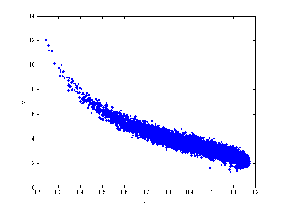
Figure 2. Distribution of $(u_{t},v_{t})$ of (2) at $t=10^{3}$. The parameters and initial value are taken as in the legend of Fig. 1.

5.2. Decline of forest

First, set $a=3,b=4,c=5,f=6,h=2,\rho=7,\sigma=4$ and take $(u_{0},v_{0})=(4,3)$. Figure 6 gives sample trajectories of $u$ and $v$ in the phase space and in time.

Second, set $a=3,b=4,c=5,f=6,h=3.82,\rho=7,\sigma=0.25$ and take $(u_{0},v_{0})=(4,3).$ By computing $5\times 10^{2}$ sample trajectories of $(u,v)$, Figure 7 shows a graph of expectation of tree densities of young and old age classes.

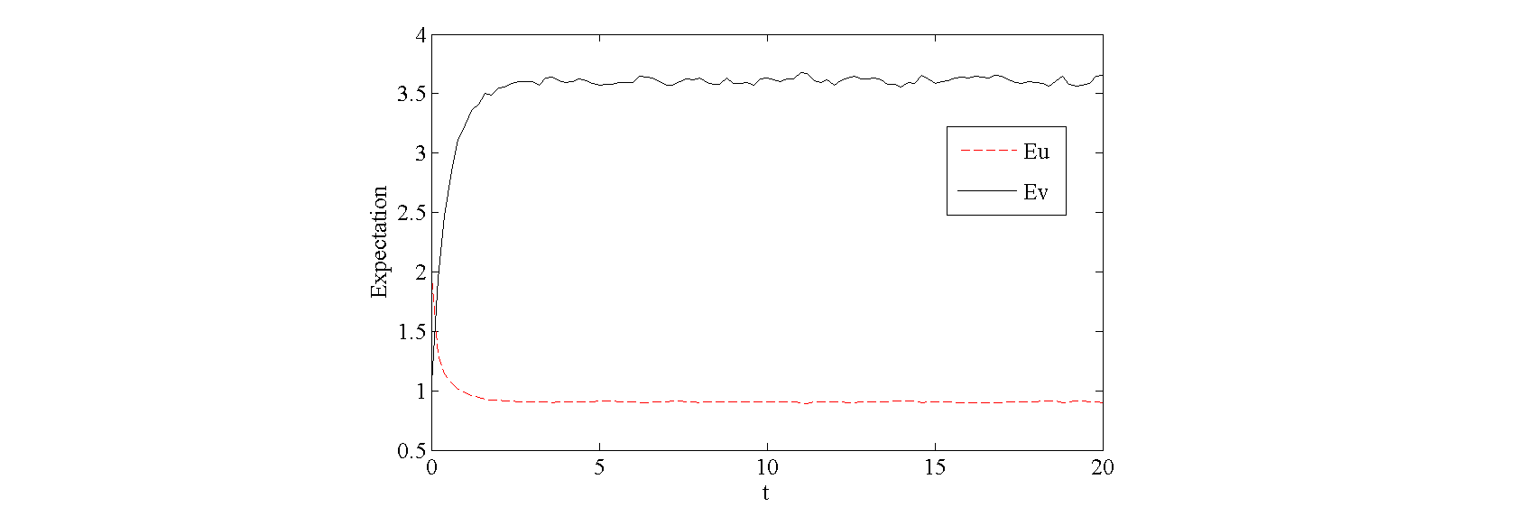
Figure 3. Graphs of $\mathbb{E}u$ and $\mathbb{E}v$ along $t\in[0,20]$. The parameters and initial value are taken as in the legend of Fig. 1.

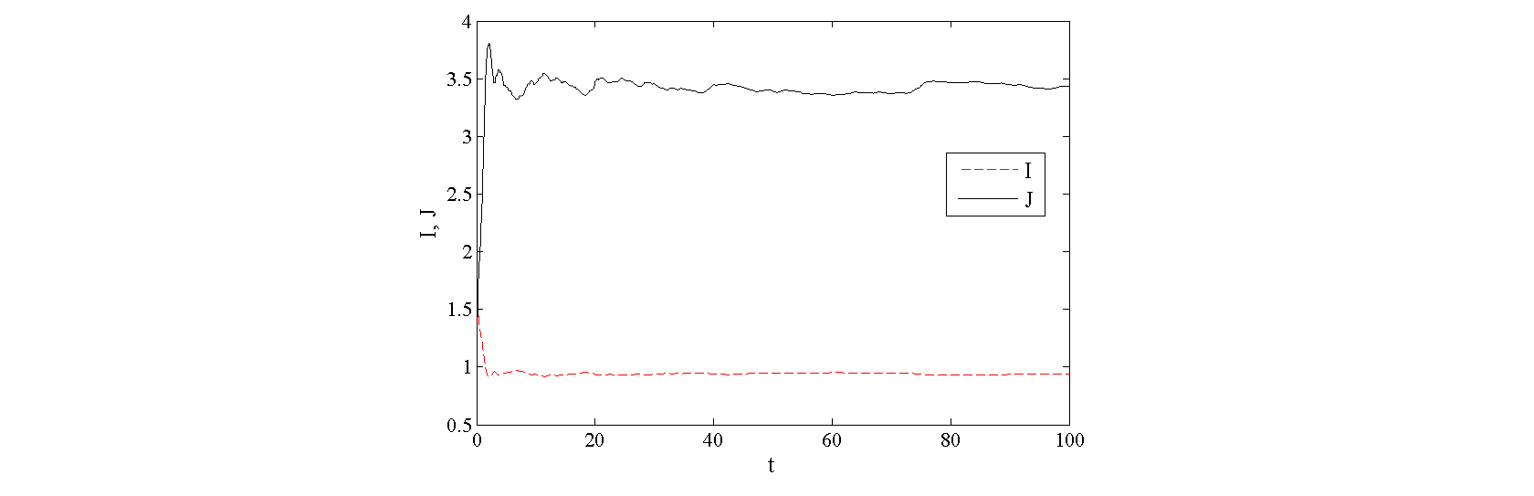
Figure 4. Sample trajectory of two processes $I$ and $J$ defined by $I(t)=\frac{1}{t}\int_{0}^{t}u_{s}ds$ and $J(t)=\frac{1}{t}\int_{0}^{t}v_{s}ds$ along $t\in[0,100].$ The parameters and initial value are taken as in the legend of Fig. 1.

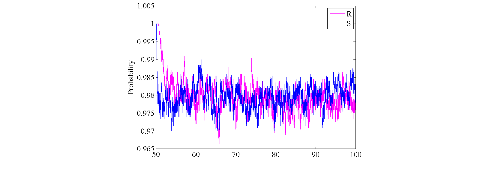
Figure 5. Graph of probability functions $R$ and $S$ defined by $R(t)=\mathbb{P}\{(u_{t},v_{t})\in A;(u_{0},v_{0})=(2,1)\}$ and $S(t)=\mathbb{P}\{(u_{t},v_{t})\in A;(u_{0},v_{0})=(3,4)\}$ along $t\in[50,100],$ where $A=[0.5,30]\times[0.1,20]$ and the parameters of (2) are taken as in the legend of Fig. 1. These functions are calculated on the basis of $2000$ sample trajectories of $(u_{t},v_{t})$ corresponding to each initial value.

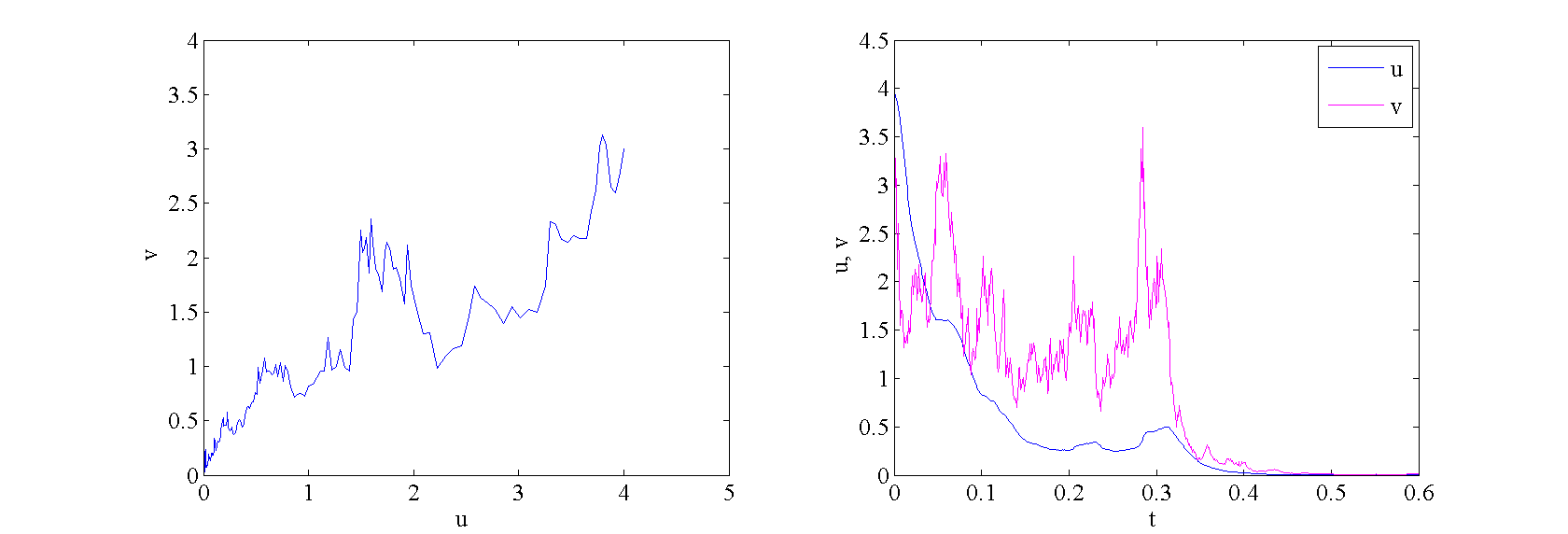
Figure 6. Decline of forest under the effect of noise with large intensity $\sigma$. Here, $a=3,b=4,c=5,f=6,h=2,\rho=7,\sigma=4$ and initial value $(u_{0},v_{0})=(4,3)$. The left figure is a sample trajectory of $(u_{t},v_{t})$ in the phase space; the right figure is a sample trajectory of $u$ and $v$ along $t\in[0,1]$.

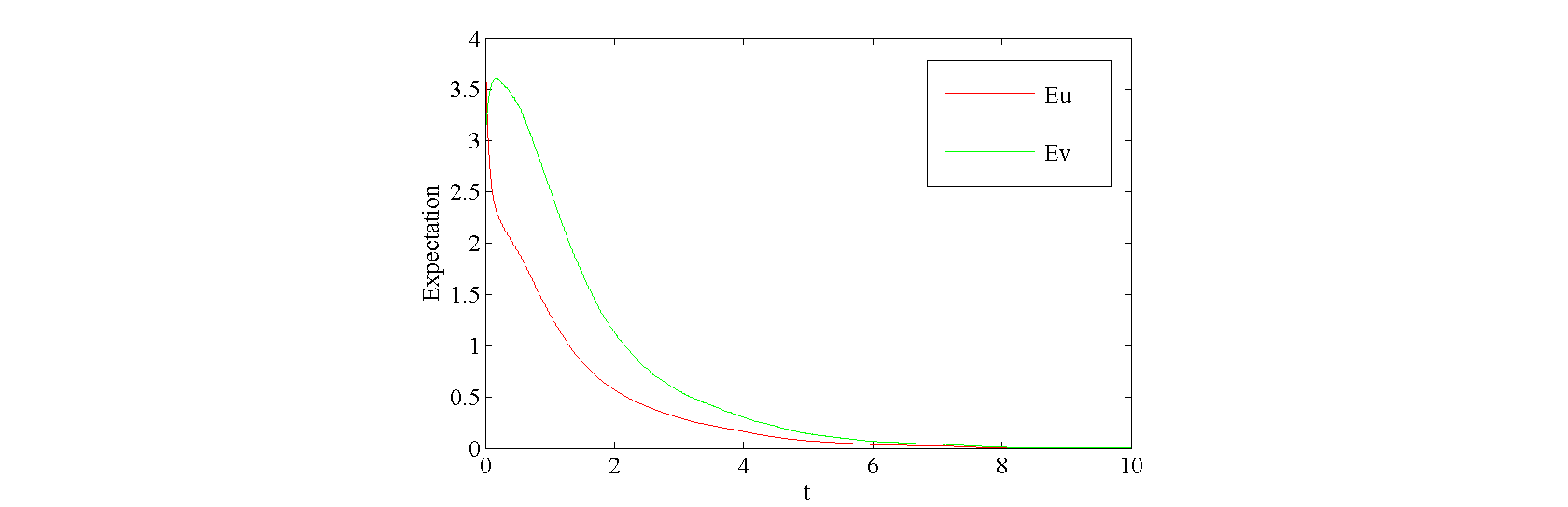
Figure 7. Decline of forest when the mortality $h$ of old trees is large. Here, $a=3,b=4,c=5,f=6,h=3.82,\rho=7,\sigma=0.25$ and initial value $(u_{0},v_{0})=(4,3).$ The figure gives a graph of $\mathbb{E}u$ and $\mathbb{E}v$ along $t\in[0,10]$.

References

- [1] M. Ya. Antonovsky, Impact of the factors of the environment on the dynamics of population (mathematical model), in Proc. Soviet-American Symp. “Comprehensive Analysis of the Environment”, Tbilisi 1974, Leningrad: Hydromet, (1975), 218–230.
- [2] (MR0443083) L. Arnold, “Stochastic Differential Equations: Theory and Applications,” Wiley, New York, 1972.
- [3] (MR2356122) L. H. Chuan and A. Yagi, Dynamical system for forest kinematic model, Adv. Math. Sci. Appl., 16 (2006), 393–409.
- [4] (MR2297947) L. H. Chuan, T. Tsujikawa and A. Yagi, Asymptotic behavior of solutions for forest kinematic model, Funkcial. Ekvac., 49 (2006), 427–449.
- [5] (MR2471671) L. H. Chuan, T. Tsujikawa and A. Yagi, Stationary solutions to forest kinematic model, Glasg. Math. J., 51 (2009), 1–17.
- [6] (MR0372154) S. R. Foguel, The ergodic theory of positive operators on continuous functions, Ann. Scuola Norm. Sup. Pisa, 27 (1973), 19–51.
- [7] (MR0494491) A. Friedman, “Stochastic Differential Equations and Applications,” Academic Press, New York, 1976.
- [8] (MR0637061) N. Ikeda and S. Watanabe, “Stochastic Differential Equations and Diffusion Processes,” North-Holland, Tokyo, 1981.
- [9] (MR1121940) I. Karatzas and S. E. Shreve, “Brownian Motion and Stochastic Calculus,” Springer-Verlag, Berlin, 1991.
- [10] (MR1260431) P. E. Kloeden, E. Platen and H. Schurz, “Numerical Solution of SDE through Computer Experiments,” Springer-Verlag, Berlin, 1994.
- [11] (MR1266986) Yu. A. Kuznetsov, M. Ya. Antonovsky, V. N. Biktashev and E. A. Aponina, A cross-diffusion model of forest boundary dynamics, J. Math. Biol., 32 (1994), 219–232.
- [12] (MR2380366) X. Mao, “Stochastic Differential Equations and Applications,” 2nd edition, Horwood, Chichester, 2008.
- [13] (MR0265559) L. Michael, Conservative Markov processes on a topological space, Isr. J. Math., 8 (1970), 165–186.
- [14] (MR2823878) L. T. H. Nguyen and T. V. Tạ, Dynamics of a stochastic ratio-dependent predator-prey model, Anal. Appl. (Singap.), 9 (2011), 329–344.
- [15] (MR2348471) T. Shirai, L. H. Chuan and A. Yagi, Asymptotic behavior of solutions for forest kinematic model under Dirichlet conditions, Sci. Math. Jpn., 66 (2007), 289–301.
- [16] (MR3150970) T. V. Tạ, L. T. H. Nguyen and A. Yagi, Flocking and non-flocking behavior in a stochastic Cucker-Smale system, Anal. Appl. (Singap.), 12 (2014), 63–73.
- [17] (MR2573296) A. Yagi, “Abstract Parabolic Evolution Equations and their Applications,” Springer-Verlag, Berlin, 2010.