Random-matrix approach to the statistical compound nuclear reaction at low energies using the Monte-Carlo technique

Abstract

Using a random-matrix approach and Monte-Carlo simulations, we generate scattering matrices and cross sections for compound-nucleus reactions. In the absence of direct reactions we compare the average cross sections with the analytic solution given by the Gaussian Orthogonal Ensemble (GOE) triple integral, and with predictions of statistical approaches such as the ones due to Moldauer, to Hofmann, Richert, Tepel, and Weidenmüller, and to Kawai, Kerman, and McVoy. We find perfect agreement with the GOE triple integral and display the limits of validity of the latter approaches. We establish a criterion for the width of the energy-averaging interval such that the relative difference between the ensemble-averaged and the energy-averaged scattering matrices lies below a given bound. Direct reactions are simulated in terms of an energy-independent background matrix. In that case, cross sections averaged over the ensemble of Monte-Carlo simulations fully agree with results from the Engelbrecht-Weidenmüller transformation. The limits of other approximate approaches are displayed.

I Introduction

For medium-weight and heavy target nuclei, nuclear reactions represent a very complex phenomenon because the number of degrees of freedom grows rapidly with mass number $A$. That fact has naturally led to the development of a statistical approach. Central to the approach are the concept of a fully equilibrated compound nucleus and the Bohr hypothesis Bohr36 , which states that a particle incident on a medium-weight or heavy nucleus shares its energy with the target nucleons. The resulting compound nucleus attains statistical equilibrium, and the modes of decay of the equilibrated system are independent of the mode of formation. The postulated independence implies a factorization of the energy-averaged compound-nucleus cross section Hauser52 . The factorization hypothesis holds very well at sufficiently large bombarding energies (i.e., in the Ericson regime) but not for isolated or weakly overlapping compound-nucleus resonances Lane57 ; Moldauer75a . In that regime the average cross section given by the factorization hypothesis must be corrected by a “width fluctuation correction” factor (WFC). The WFC factor basically accounts for an enhancement of the elastic average cross section.

In the 1970s numerous efforts were undertaken to derive the WFC factor Moldauer75a ; Moldauer75b ; Kawai73 ; Agassi75 ; Hofmann75 ; Mello79 ; Mello80 or to generate a suitable parametrization of the WFC factor with the help of the Monte-Carlo (MC) technique Hofmann75 ; Hofmann80 ; Moldauer78 ; Moldauer80 . All of these were guided by random-matrix theory (RMT). Inspired by Bohr’s idea, Wigner had introduced RMT into nuclear physics as a means to cope with the complexities of the compound nucleus (see Brody et al. Brody81 ). In RMT, the nuclear Hamiltonian is assumed to be a member of the Gaussian Orthogonal Ensemble (GOE) of random matrices. Wigner himself never went as far as formulating a statistical theory of nuclear reactions in terms of the GOE. Lacking such a theory, the above-mentioned approaches used approximations that were not fully controlled. Only in 1985 an exact closed-form expression for the average $S$ matrix and for the $S$ matrix correlation function based upon a GOE scattering approach was derived Verbaarschot85 , based upon the shell-model approach to nuclear reactions Mahaux69 and valid in the limit of a large number of resonances. In that work the $S$ matrix is written in terms of the GOE Hamiltonian $H^{({\rm GOE})}$. Averages are performed directly over the Gaussian-distributed elements of $H^{({\rm GOE})}$.

The exact results of the GOE scattering approach Verbaarschot85 apply for all values of the parameters (number of open channels, isolated or overlapping resonances) characterizing compound-nucleus reactions. More generally, that work describes universal features of quantum-chaotic scattering Weidenmueller09 ; Mitchel10 and is, therefore, relevant also beyond the confines of nuclear physics. However, the exact expression for the $S$-matrix correlation function Verbaarschot85 involves a triple integral. The computational cost of evaluating that integral is quite heavy especially when many channels are open. That is why only few numerical studies have been performed in the past. Fröhner Frohner89 and Igarasi Igarasi91 independently compared the GOE triple integral results with Moldauer’s method, and obtained good agreement. Hilaire, Lagrange, and Koning Hilaire03 extended the numerical study, and applied it to some realistic cases where neutron radiative capture and fission channels are involved. Updated parametrizations of Moldauer’s method based on the GOE triple integral calculation are also available Ernebjerg04 ; Kawano13 , which are of practical use for cross-section calculations.

In the present paper we present a thorough analysis of the results of the GOE approach and a comparison with other, approximate methods, with the aim to understand their applicability and limitation. The work is based upon a Monte-Carlo approach. We generate an ensemble of scattering matrices or cross sections. This is done by drawing at random the elements of $H^{({\rm GOE})}$ and using these to generate the elements of the scattering matrix. In this way we are able to avoid some phenomenological assumptions made in the past concerning the distribution of the decay amplitudes or of levels. In that respect our MC approach also differs from the one used by Moldauer or Hofmann et al. We average over the ensemble of realizations generated by the MC method and compare these with predictions of the exact GOE approach and of other approximate methods. We are able to answer some important and long-standing questions concerning compound nuclear reactions, such as the difference between energy and ensemble averages, the role of direct channels, the existence of correlations between distributions of levels and decay amplitudes, and the behavior of the cross section in the limit of weak absorption.

II Theory of stochastic scattering

II.1 Compound-nucleus cross section

The cross section for a reaction from channel $a$ to channel $b$ is written as

$$\sigma_{ab}=\frac{\pi}{k_{a}^{2}}g_{a}|\delta_{ab}-S_{ab}|^{2}\ .$$ (1)

Here $k_{a}$ is the wave number for channel $a$, $g_{a}$ is the spin factor, and the element $S_{ab}$ of the scattering matrix $S$ consists of an energy-averaged part $\langle S_{ab}\rangle$ and a fluctuating part $S_{ab}^{{\rm fl}}$. The energy-averaged cross section also consists of two parts,

$$\langle\sigma_{ab}\rangle = \frac{\pi}{k_{a}^{2}}g_{a}\langle|\delta_{ab}-S_{ab}|^{2}\rangle$$ (2)

$$= \frac{\pi}{k_{a}^{2}}g_{a}\left\{|\delta_{ab}-\langle S_{ab}\rangle|^{2}+\langle|S_{ab}^{{\rm fl}}|^{2}\rangle\right\}\ .$$

The term containing $|\delta_{ab}-\langle S_{ab}\rangle|^{2}$ describes shape elastic ($a=b$) or shape inelastic ($a\neq b$) scattering. The term containing $\langle|S_{ab}^{{\rm fl}}|^{2}\rangle$ is the average compound-nucleus (CN) cross section

$$\sigma^{\rm CN}_{ab}=\frac{\pi}{k_{a}^{2}}g_{a}\langle|S^{\rm fl}_{ab}|^{2}\rangle\ .$$ (3)

In the first part of the paper we confine ourselves to cases where the average $S$ matrix is diagonal, $\langle S_{ab}\rangle=\delta_{ab}\langle S_{aa}\rangle$. Then $\langle S_{aa}\rangle$ and the shape-elastic cross section

$$\sigma^{\rm SE}_{aa}=\frac{\pi}{k_{a}^{2}}g_{a}|1-\langle S_{aa}\rangle|^{2}$$ (4)

are given by the optical model. It is the aim of various theories of CN reactions to express the CN cross section in terms of $\langle S_{aa}\rangle$ and of the transmission coefficients

$$T_{a}=1-|\langle S_{aa}\rangle|^{2}\ ,\ \quad 0\leq T_{a}\leq 1\ .$$ (5)

These measure the unitary deficit of $\langle S\rangle$ and, thus, the probability of CN formation. In the second part of the paper we address the case when $\langle S_{ab}\rangle$ is not diagonal.

Bohr’s idea of the independence of formation and decay of the CN led to the Hauser-Feshbach formula Hauser52 for the CN cross section,

$$\sigma^{\rm HF}_{ab}=\frac{\pi}{k_{a}^{2}}g_{a}\frac{T_{a}T_{b}}{\sum_{c}T_{c}}\ .$$ (6)

Corrections to that formula are conveniently expressed in terms of the “width fluctuation correction” (WFC) factor Moldauer61 ,

$$\sigma^{\rm CN}_{ab}=\frac{\pi}{k_{a}^{2}}g_{a}\frac{T_{a}T_{b}}{\sum_{c}T_{c}}W_{ab}\ .$$ (7)

Rigorously speaking, $W_{ab}$ should be separated into two parts, the “elastic enhancement factor” and the proper “width fluctuation correction factor” Moldauer75a . However, for the comparison of various approaches it is more convenient to adopt the suggestion of Hilaire, Lagrange, and Koning Hilaire03 and to define the width fluctuation factor $W_{ab}$ as the ratio $\sigma^{\rm CN}_{ab}/\sigma^{\rm HF}_{ab}$.

In what follows we compare several approaches to the calculation of $\sigma^{\rm CN}_{ab}$ and/or of the WFC factor. In chronological order, these are the approach of Kawai, Kerman, and MacVoy Kawai73 (KKM), the parametrization by Hofmann, Richert, Tepel, and Weidenmüller Hofmann75 (HRTW), Moldauer’s parametrization Moldauer80 , the GOE approach by Verbaarschot, Weidenmüller, and Zirnbauer Verbaarschot85 , the parametrization by Ernebjerg and Herman Ernebjerg04 , and that by Kawano and Talou Kawano13 . These are briefly summarized in the Appendix. Hereafter we drop the kinetic and spin factors $\pi g_{a}/k_{a}^{2}$, so that all the cross sections are dimensionless.

All these approaches use GOE-inspired statistical assumptions on the parameters of the CN resonances. In our comparison we use the results of Ref. Verbaarschot85 as a benchmark. We do so because the work of Ref. Verbaarschot85 is the only one that, starting from a random-matrix model for the Hamiltonian of the CN resonances and using controlled approximations, obtains an analytical expression for $\sigma^{\rm CN}_{ab}$ that is valid in all regimes — from the regime of isolated resonances to that of strongly overlapping resonances.

II.2 $S$ matrix, $K$ matrix, $R$ matrix

In order to display the connection between various theories of resonance reactions we recall here briefly the derivation of a universal expression for the $S$ matrix Mahaux69 ; Kawai73 . Specialization of that expression then yields the formulas used in various approaches.

Given a time-reversal-invariant Hamiltonian $H$ we use Feshbach’s projection operators $P$ and $Q=1-P$ (where $P$ projects onto all open channels labelled $a,b,\ldots$) to write the Schrödinger equation $(E-H)\Psi=0$ for the scattering wave function $\Psi$ in the form of the coupled equations

$$(E-H_{PP})P\Psi = H_{PQ}Q\Psi\ ,$$ (8)

$$(E-H_{QQ})Q\Psi = H_{QP}P\Psi\ .$$ (9)

We use the standard notation, $H_{PP}=PHP$, $H_{PQ}=PHQ$, etc. With the $P$ space scattering wave function $\psi_{a}^{(+)}$ defined by

$$(E-H_{PP})\psi_{a}^{(+)}=0\ ,$$ (10)

the unitary and symmetric $S$ matrix is given by

$$S_{ab}=S_{ab}^{(0)}-2\pi i\left(\psi_{a}^{(-)}|H_{PQ}\frac{1}{E-{\cal H}_{QQ}}H_{QP}|\psi_{b}^{(+)}\right)\ .$$ (11)

Here $S_{ab}^{(0)}$ is a unitary background scattering matrix defined by the asymptotic form of the solutions $\psi_{a}^{(+)}$, and ${\cal H}_{QQ}$ is the effective Hamiltonian in $Q$ space,

$${\cal H}_{QQ}=H_{QQ}+H_{QP}\frac{1}{E^{+}-H_{PP}}H_{PQ}\ .$$ (12)

To be useful Eqs. (11) and (12) must be specialized further. The $S$-matrix approach of Ref. Verbaarschot85 and the expressions for $S$ in terms of the $K$ matrix and the $R$ matrix use different such specializations. Common to these is the assumption that the unitary background scattering matrix $S^{(0)}$ is diagonal, $S^{(0)}_{ab}=\delta_{ab}\exp\{2i\phi_{a}\}$. We assume that the phases $\phi_{a}$ are removed by the transformation $S_{ab}\to\exp\{-i\phi_{a}\}S_{ab}\exp\{-i\phi_{b}\}$. Then $\psi^{(+)}_{a}\exp\{-i\phi_{a}\}=\psi_{a}$ is real, and Eq. (11) becomes

$$S_{ab}=\delta_{ab}-2\pi i\left(\psi_{a}|H_{PQ}\frac{1}{E-{\cal H}_{QQ}}H_{QP}|\psi_{b}\right)\ .$$ (13)

For the $S$-matrix approach of Ref. Verbaarschot85 we introduce an arbitrary orthonormal basis of states labeled $\mu$ in $Q$ space and write

$$W_{\mu a}=(\mu|H_{QP}|\psi_{a})=W_{a\mu}=W^{*}_{a\mu}\ ,$$ (14)

$$\left(\mu|H_{QP}\frac{1}{E^{+}-H_{PP}}H_{PQ}|\nu\right)=\Delta_{\mu\nu}-i\pi\sum_{c}W_{\mu c}W_{c\nu}\ ,$$ (15)

$$\left(\mu|H_{QQ}|\nu\right)=H_{\mu\nu}\ .$$ (16)

The sum extends over all open channels. The real shift function $\Delta_{\mu\nu}$ is defined by a principal-value integral. It is commonly assumed that the matrix elements $W_{a\mu}$ change slowly with energy on a scale defined by the mean level spacing of the resonances. Then $\Delta_{\mu\nu}\approx 0$. We use that assumption throughout. With these definitions, Eqs. (11) and (12) take the form

$$S_{ab}=\delta_{ab}-2i\pi\sum_{\mu\nu}W_{a\mu}(D^{-1})_{\mu\nu}W_{\nu b}$$ (17)

where

$$D_{\mu\nu}=E\delta_{\mu\nu}-H_{\mu\nu}+i\pi\sum_{c}W_{\mu c}W_{c\nu}\ .$$ (18)

For the $K$-matrix parametrization of $S$ we use Eq. (12) to define the eigenvalues $E_{\sigma}$ and eigenvectors $X_{\sigma}$ of the bound compound system,

$$(E_{\sigma}-H_{QQ})X_{\sigma}=0\ .$$ (19)

The states $X_{\sigma}$ produce the CN resonances in the scattering process. These states correspond to a special choice of the basis of states $\mu$ used in Eqs. (14)–(16). The partial decay amplitude of state $X_{\sigma}$ into channel $a$ is

$$\gamma_{\sigma a}=\gamma^{*}_{\sigma a}=(X_{\sigma}|H_{QP}|\psi_{a})\ .$$ (20)

Under neglect of the shift matrix $\Delta$ the $S$ matrix of Eq. (13) can be written as

$$S_{ab}=\bigg{(}\frac{1-iK}{1+iK}\bigg{)}_{ab}$$ (21)

where

$$K_{ab}(E)=\pi\sum_{\sigma}\frac{\gamma_{a\sigma}\gamma_{\sigma b}}{E-E_{\sigma}}\ .$$ (22)

The $R$ matrix is obtained by a non-standard choice of the projection operators $P$ and $Q$. In every channel $c$ (open and closed) a radius $r_{c}$ is defined. The set $\{r_{c}\}$ of all channel radii separates the internal and the external regions of configuration space. The operator $Q$ projects onto the internal region, and $P=1-Q$. At the channel surfaces of the internal region, self-adjoint boundary conditions are introduced with real boundary condition parameters $B_{c}$. These define a Hermitian Hamiltonian $H_{QQ}$ and associated internal eigenvalues $E^{({\rm R})}_{\sigma}$ and orthonormal eigenfunctions $X^{({\rm R})}_{\sigma}$. The reduced width amplitude $\gamma^{({\rm R})}_{\sigma c}$ is the projection of the eigenfunction $X^{({\rm R})}_{\sigma}$ onto the surface of channel $c$, and the $R$ matrix is defined as

$$R_{ab}(E)=\sum_{\sigma}\frac{\gamma^{({\rm R})}_{a\sigma}\gamma^{({\rm R})}_{\sigma b}}{E^{({\rm R})}_{\sigma}-E}\ .$$ (23)

This is in close analogy to Eq. (22), except that a factor $\sqrt{\pi}$ has been absorbed by each of the reduced width amplitudes. The resulting form of the scattering matrix is

$$S_{ab} = \delta_{ab}$$ (24)

$$+ 2i\sqrt{P_{a}}\left(\{1-R(L-B)\}^{-1}R\right)_{ab}\sqrt{P_{b}}\ .$$

Here $P_{a}$ is the penetration factor in channel $a$, the matrices $B$ and $L$ are diagonal with elements $B_{a}$ and $L_{a}={\cal S}_{a}+iP_{a}$, and the real entities ${\cal S}_{a}-B_{a}$ play a role that is analogous to that of the shift function $\Delta$ in Eq. (15). The diagonal matrices $L$ and $P$ depend only on channel radius $r_{a}$ and wave number $k_{a}$ Moldauer64 . The boundary condition parameter $B_{a}$ is often taken as $B_{a}=-l_{a}$ Wigner47 , with $l_{a}$ the orbital angular momentum of relative motion in channel $a$. In the $R$-matrix approach the phases $\phi_{a}$ are caused by elastic scattering on a hard sphere of radius $r_{a}$ while in the approach of Ref. Verbaarschot85 they are elastic potential scattering phase shifts.

II.3 Implementation of stochasticity

To fully define the scattering matrices in Sec. II.2 we need to determine the resonance parameters. This is done by introducing statistical assumptions, using random-matrix theory Mehta04 as a guiding principle. The actual procedure is somewhat different for the three forms of the scattering matrix in Sec. II.2. These are referred to as the $S$-matrix approach, the $K$-matrix approach, and the $R$-matrix approach, respectively.

The relevant random-matrix ensemble is the time-reversal-invariant Gaussian Orthogonal Ensemble (GOE). The elements $H^{({\rm GOE})}_{\mu\nu}$ of the $N$-dimensional GOE matrix $H^{({\rm GOE})}$ are Gaussian-distributed real random variables with zero mean values and second moments given by

$$\overline{H_{\mu\nu}^{({\rm GOE})}H_{\rho\sigma}^{({\rm GOE})}}=\frac{\lambda^{2}}{N}(\delta_{\mu\rho}\delta_{\nu\sigma}+\delta_{\mu\sigma}\delta_{\nu\rho})\ .$$ (25)

Here and in what follows, the ensemble average is denoted by an overbar. The parameter $\lambda$ is related to the average level spacing $d$ at the center of the GOE spectrum by $d=\pi\lambda/N$. Universal properties are analytically derived Mehta04 in the limit $N\to\infty$. These are: The eigenvalues and the eigenvectors of $H^{({\rm GOE})}$ are statistically uncorrelated. The projections of the (real) eigenvectors on any fixed vector in Hilbert space have a Gaussian distribution centered at zero. The eigenvalues obey Wigner-Dyson statistics. The degree to which these properties can be implemented depends on the approach used.

In the $S$-matrix approach the $Q$-space Hamiltonian $H_{\mu\nu}$ of Eq. (18) is replaced by $H^{({\rm GOE})}_{\mu\nu}$. That replacement provides the most direct implementation of random-matrix theory into scattering theory. The average cross section is worked out as an average over the GOE. For the specification of the parameters $W_{a\mu}$ one uses the invariance of the GOE under orthogonal transformations in Hilbert space. That invariance implies that ensemble averages can depend on the $W$’s only via the invariant forms $\sum_{\mu}W_{a\mu}W_{\mu b}$. For the average $S$ matrix to be diagonal, the sums must be diagonal in the channel indices,

$$\sum_{\mu}W_{a\mu}W_{\mu b}=\delta_{ab}Nv^{2}_{a}\ ,$$ (26)

and the only parameters left are the $v^{2}_{a}$. With

$$x_{a}=\frac{\pi^{2}v^{2}_{a}}{d}\ ,$$ (27)

these determine the average $S$ matrix elements $\overline{S}_{aa}$ and the transmission coefficients $T_{a}$ as

$$\overline{S}_{aa}=\frac{1-x_{a}}{1+x_{a}}\ ,\qquad T_{a}=\frac{4x_{a}}{(1+x_{a})^{2}}\ .$$ (28)

Equations (28) imply that the average strength $x_{a}$ of the coupling of the CN resonance states to channel $a$ is fixed by the average $S$ matrix and, thus, determined by the shape-elastic input. In that sense, the GOE ensemble average of $|S^{\rm fl}_{ab}|^{2}$ is parameter-free. This is different from past calculations using a statistical $R$ matrix or $K$ matrix.

In the $K$-matrix and $R$-matrix approaches, two assumptions are made:

1. The partial width amplitudes $\gamma_{a\sigma}$ and the reduced width amplitudes $\gamma^{({\rm R})}_{a\sigma}$ both have a Gaussian distribution with zero mean and a specified second moment $\langle\gamma_{a}^{2}\rangle$.

2. The eigenvalues $E_{\sigma}$ and $E^{({\rm R})}_{\sigma}$ obey Wigner-Dyson statistics.

If fully implemented, these assumptions correspond for $N\to\infty$ to the properties of the GOE listed below Eq. (25).

In practical calculations, the implementation of these statistical assumptions causes difficulties. The $S$-matrix approach lends itself to an analytical calculation of $\sigma^{{\rm CN}}_{ab}$ in the limit $N\to\infty$. The resulting expression is given in Eq. (35) below. However, the use of that expression was limited for a long time because of the difficulties in calculating reliably the ensuing threefold integral. A direct implementation would consist in drawing the elements $H^{({\rm GOE})}_{\mu\nu}$ from a Gaussian distribution, choosing a set of matrix elements $W_{a\mu}$ consistent with Eqs. (26) and (28), and inverting the resulting matrix $D_{\mu\nu}$. For $N\gg 1$ that is quite cumbersome and, to the best of our knowledge, has not been done before. We report on such a calculation below.

For the $K$-matrix and $R$-matrix approaches, it is straightforward to draw the partial width amplitudes or the reduced width amplitudes from a Gaussian distribution. To meet postulate 2, the eigenvalues should be determined by diagonalization of the GOE matrix $H^{({\rm GOE})}$ for $N\gg 1$. This is cumbersome, and a simplified version sometimes replaces postulate 2. The Wigner surmise for the distribution $P(s)$ of spacings $s$ of neighboring eigenvalues reads

$$P_{W}(s)=\frac{\pi}{2}s\exp\left(-\frac{\pi s^{2}}{4}\right)\ ,$$ (29)

with $s$ the actual spacing in units of $d$. Spacings of neighboring eigenvalues are drawn at random from $P_{W}(s)$ and are used to construct the spectrum. Higher correlations between eigenvalue spacings are thereby neglected. In particular, the stiffness of the GOE spectrum (a central property) is not taken into account.

With this input, the energy-averaged cross section $\langle|\delta_{ab}-S_{ab}|^{2}\rangle$ can be calculated. It is often assumed that the energy average can be replaced by an ensemble average over the joint distribution of level energies and decay amplitudes. The ensemble average can be readily obtained even in the limit of isolated resonances. The energy-averaged $S$ matrix is more simply obtained using a Lorentzian average of width $I$ and given by

$$\langle S(E)\rangle=S(E+iI)\ ,$$ (30)

and $S(E+iI)$ is obtained by replacing $K(E)$ in Eq. (22) or $R(E)$ in Eq. (23) by $K(E+iI)$ or $R(E+iI)$, respectively. That yields the transmission coefficients in Eq. (5).

Monte Carlo calculations based on this approach Frohner00 have been used to define heuristic parametrizations of the width fluctuation correction factor $W_{ab}$. The results of Hofmann, Richert, Tepel, and Weidenmüller Hofmann75 ; Hofmann80 (HRTW) are based on the $K$ matrix, those of Moldauer Moldauer80 on the $R$ matrix. The resulting fit formulas for the WFC factor are collected in the Appendix.

III Monte-Carlo simulations

III.1 $R$ matrix and $S$ matrix

In the 1960s and 70s, the statistical $R$-matrix approach used by Moldauer Moldauer75a ; Moldauer75b offered the only possibility to use random-matrix ideas in CN scattering. As an example for that method we show in Fig. 1 the result of a new Monte-Carlo simulation of the elastic cross section for neutron scattering on ⁵⁶Fe (bottom panel). This is compared with the real cross section (upper panel) given in ENDF/B-VII.1 ENDF7 . In the simulation we put $\langle\gamma_{c}^{2}\rangle=10$ keV for the $s$ wave, and 200 eV for the higher partial waves ($p$, $d$, and $f$ waves). The radiative capture channel was ignored. Although the statistical $R$-matrix calculation cannot reproduce the detailed structure, the comparison provides information on average properties and, thus, a useful link between the fluctuating cross section and the optical model calculations Kawano97 .

However, the approach involves a number of parameters, such as the partial widths, the level density Gilbert65 ; Kawano06 , the energy range of interest, and so forth. Strict implementation of the more abstract GOE approach actually removes the need to define these parameters. This is most easily demonstrated for the case of the $K$ matrix. Upon scaling the energies by the mean level spacing $d$ so that $E/d\to\epsilon$, $E_{\sigma}/d\to\epsilon_{\sigma}$, the quantities $\epsilon$ and $\epsilon_{\sigma}$ are dimensionless, and the spacing distribution of the $\epsilon_{\sigma}$ is given in terms of the universal dimensionless correlation functions of the GOE Mehta04 . The expression for $P_{W}(s)$ in Eq. (29) is an example. Applying the analogous scaling to the partial width amplitudes, $\gamma_{a\sigma}/d^{1/2}\to\tilde{\gamma}_{a\sigma}$ generates dimensionless uncorrelated Gaussian-distributed random variables $\tilde{\gamma}_{a\sigma}$. The second moments of these quantities are determined by the average $S$-matrix elements of the optical model. In other words, the scaling $E/d\to\epsilon$, $E_{\sigma}/d\to\epsilon_{\sigma}$, $\gamma_{a\sigma}/d^{1/2}\to\tilde{\gamma}_{a\sigma}$ maps the CN scattering problem onto a GOE scattering problem where the only input parameters are the number of open channels and the elements $\langle S_{aa}\rangle$ of the average scattering matrix in each channel. That scattering problem describes universal chaotic scattering.

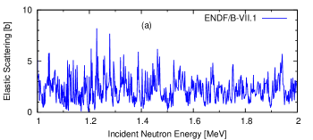
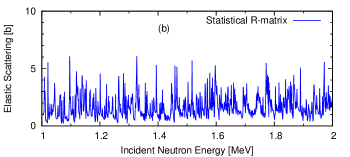
Figure 1: (Color Online) An example of an elastic scattering cross section generated with the statistical $R$-matrix method (bottom panel), compared with the real cross section in ENDF/B-VII.1 (top panel), for a neutron-induced reaction on ⁵⁶Fe in the 1–2 MeV energy range.

For the $S$-matrix simulation, Eqs. (17) and (18) with $H_{\mu\nu}$ replaced by $H^{({\rm GOE})}_{\mu\nu}$ as

$$S_{ab}^{({\rm GOE})} = \delta_{ab}-2i\pi\sum_{\mu\nu}W_{a\mu}\left(D^{-1}\right)_{\mu\nu}W_{\nu b}\ ,$$ (31)

$$D_{\mu\nu} = E\delta_{\mu\nu}-H_{\mu\nu}^{({\rm GOE})}+i\pi\sum_{c}W_{\mu c}W_{c\nu}\ ,$$ (32)

serve as starting point. The matrix elements $W_{\mu a}$ obey Eq. (26). The simulation generates an ensemble of $S$ matrices by generating a single set of matrix elements $\{W_{\mu a}\}$ combined with a number of realizations of $H^{({\rm GOE})}$. By construction, all $S$ matrices in the ensemble have for $N\to\infty$ the same mean values. The matrix elements $W_{\mu a}$ are determined as follows. Given the elements $G_{\mu a}$ of a coupling strength matrix $G$ of dimension $N\times\Lambda$, where $\Lambda$ is the number of channels, diagonalization of the real symmetric matrix $G^{T}G$ in channel space with an orthogonal matrix ${\cal O}$ yields

$${\cal O}^{-1}G^{T}G{\cal O} = \mbox{diag}(v_{a}^{2})\ ,$$ (33)

$$W = G{\cal O}\ .$$ (34)

This procedure guarantees that Eqs. (26) are satisfied. The eigenvalues $v_{a}^{2}$ and $d=\pi\lambda/N$ define $x_{a}=\pi^{2}v^{2}_{a}/d$ and these, in turn, the transmission coefficients $T_{a}$ via Eq. (28). Figure 2 shows examples of calculated elastic scattering cross sections for $\Lambda=2$, $N=20,100$, and for three different transmission coefficients $T_{a}=0.1$, $0.5$, and $0.99$. To show how the cross section evolves as the transmission coefficient increases, we fixed the random number sequence so that the eigenvalues of $H^{\rm(GOE)}$ are the same for the three $T_{a}$ cases.

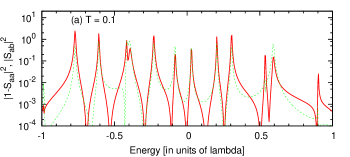
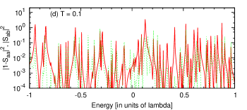
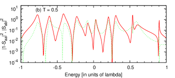
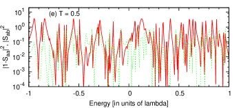
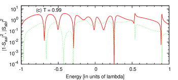
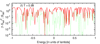
Figure 2: (Color Online) Generated elastic $|1-S_{aa}|^{2}$ and inelastic $|S_{ab}|^{2}$ scattering cross sections with the GOE $S$-matrix for three different transmission coefficients $T_{a}$ of 0.1, 0.5, and 0.99. The solid curves are the elastic, and the dotted curves are the inelastic cross sections. The left column is for $N=20$ and the right is for the $N=100$ case.

III.2 Ensemble average

The ensemble average of Eqs. (31) and (32) can be evaluated numerically either by employing the MC technique where the elements $H^{({\rm GOE})}$ are drawn from a Gaussian distribution, or by calculating the three-fold integral of Verbaarschot, Weidenmüller, and Zirnbauer Verbaarschot85

$$\overline{S_{ab}^{\rm fl}(E_{1})S_{cd}^{{\rm fl}*}(E_{2})} = \frac{1}{8}\int_{0}^{\infty}d\lambda_{1}\int_{0}^{\infty}d\lambda_{2}\int_{0}^{1}d\lambda\quad\mu(\lambda,\lambda_{1},\lambda_{2})$$ (35)

$$\times e^{-ir(\lambda_{1}+\lambda_{2}+2\lambda)}{\displaystyle\prod_{c}}\frac{1-T_{c}\lambda}{\sqrt{(1+T_{c}\lambda_{1})(1+T_{c}\lambda_{2})}}J(\lambda,\lambda_{1},\lambda_{2})\ ,$$

where

$$\mu(\lambda,\lambda_{1},\lambda_{2}) = \frac{\lambda(1-\lambda)|\lambda_{1}-\lambda_{2}|}{\sqrt{\lambda_{1}(1+\lambda_{1})}\sqrt{\lambda_{2}(1+\lambda_{2})}(\lambda+\lambda_{1})^{2}(\lambda+\lambda_{2})^{2}}\ ,$$ (36)

$$J(\lambda,\lambda_{1},\lambda_{2}) = \delta_{ab}\delta_{cd}\overline{S}_{aa}\overline{S}_{cc}^{*}T_{a}T_{c}\left(\frac{\lambda_{1}}{1+T_{a}\lambda_{1}}+\frac{\lambda_{2}}{1+T_{a}\lambda_{2}}+\frac{2\lambda}{1-T_{a}\lambda}\right)\left(\frac{\lambda_{1}}{1+T_{c}\lambda_{1}}+\frac{\lambda_{2}}{1+T_{c}\lambda_{2}}+\frac{2\lambda}{1-T_{c}\lambda}\right)$$ (37)

$$+ (\delta_{ac}\delta_{bd}+\delta_{ad}\delta_{bc})T_{a}T_{b}\left\{\frac{\lambda_{1}(1+\lambda_{1})}{(1+T_{a}\lambda_{1})(1+T_{b}\lambda_{1})}+\frac{\lambda_{2}(1+\lambda_{2})}{(1+T_{a}\lambda_{2})(1+T_{b}\lambda_{2})}+\frac{2\lambda(1+\lambda)}{(1-T_{a}\lambda)(1-T_{b}\lambda)}\right\}\ ,$$

$$r = \frac{\pi}{d}(E_{2}-E_{1})\ .$$ (38)

The triple-integral in Eq. (35) can be evaluated numerically by introducing new integration variables Verbaarschot86 that avoid singularities in the integrand, and by the Gauss-Legendre quadrature with the order high enough to obtain convergence Hilaire03 . In practical applications we need $\overline{S_{ab}S_{ab}^{*}}$ only, so that Eq. (35) can be reduced to a slightly simpler form Hilaire03 as $\overline{S}_{aa}\overline{S}_{aa}^{*}=1-T_{a}$. This is not the case if we have off-diagonal elements in $\langle S\rangle$, or different energy arguments so that $r\neq 0$.

A benefit of MC is that we are able to explore a larger parameter space, while Eq. (35) holds in the limit $N\rightarrow\infty$. In Eq. (35) we have replaced the energy average $\langle|\delta_{ab}-S_{ab}^{({\rm GOE})}|^{2}\rangle$ by the ensemble average $\overline{|\delta_{ab}-S_{ab}^{({\rm GOE})}|^{2}}$. The difference between the two averages is discussed later. Hereafter we always calculate the ensemble average unless stated explicitly otherwise. The average is evaluated at the center of the GOE eigenvalue distribution, $E=0$. As shown in Fig. 2, the calculated cross section near $E=0$ for a single realization of $H^{({\rm GOE})}$ displays chaotic fluctuations. The number of MC realizations needed to obtain a meaningful average varies from 10,000 to a million, depending on convergence. The criterion used was that the deviation of the average $S$-matrix from its input value was sufficiently small, $|\Delta\overline{S}_{ab}|<10^{-5}$.

Figure 3 shows the probability distribution of the elastic scattering cross section at $E=0$ for $N=100$, $\Lambda=2$, and three different $T_{a}=T_{b}$ values of 0.1, 0.5, and 0.99. The MC ensemble average values are indicated by the location of the arrows, e.g., in the case of $T_{a}=0.99$, the average is 1.47. To compare these averages with predictions of the statistical model, we have to subtract the direct part $(1-\Re\overline{S}_{aa})^{2}$ from the elastic channel. That gives the average fluctuating part $\overline{|S^{\rm fl}|^{2}}$ of 0.660. The Hauser-Feshbach cross section is

$$\langle|S_{aa}^{\rm fl}|^{2}\rangle=\frac{T_{a}^{2}}{T_{a}+T_{b}}=0.495\ ,$$ (39)

giving in that case a 25% smaller elastic cross section. When the GOE triple-integral of Eq. (35) is performed for the given transmission coefficients, the simulated cross sections are recovered. In Table 1 we compare the MC results with other statistical models — KKM Kawai73 , HRTW Hofmann75 ; Hofmann80 , Moldauer Moldauer80 , Ernebjerg and Herman Ernebjerg04 , and Kawano and Talou Kawano13 . In general, all the statistical models predict the average reasonably well when $\langle\Gamma\rangle/d$ is large. More comparisons of the MC generated cross sections with these statistical models can be found in Ref. Kawano13 .

One may argue that the agreement between the GOE triple-integral and the MC simulation is obvious because the triple-integral is an analytical form of the ensemble average for Eqs. (31) and (32) in the limit of $N\rightarrow\infty$. We have, therefore, studied the $N$-dependence of the calculated averages. Starting with $N=100$, we reduce the number of resonances and compare the ensemble average of the elastic cross section with the triple-integral results. Surprisingly the triple-integral still gives very accurate average values even if $N=3$. Averaging over a few resonances is certainly an extreme case, and is not realistic.

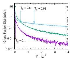
Figure 3: (Color Online) Distribution of elastic scattering cross section at $E=0$ for many GOE $S$-matrix realizations. Three cases, $T_{a}=T_{b}=0.1$, 0.5, and 0.99 are shown. The arrows show the actual average values for each distribution.

Table 1: Comparison of numerical average $\overline{|S_{aa}^{\rm fl}|^{2}}$ for some cases of $T_{a}=T_{b}=0.1$, 0.5, and 0.99, with the statistical models — Hauser-Feshbach Hauser52 , KKM Kawai73 , HRTW Hofmann80 , Moldauer Moldauer80 , GOE Verbaarschot85 , Ernebjerg-Herman Ernebjerg04 , and Kawano-Talou Kawano13 .

$T_{a}$	0.1		0.5		0.99
	Elastic	Inelastic	Elastic	Inelastic	Elastic	Inelastic
MC simulation	0.0733	0.0261	0.351	0.149	0.660	0.330
Hauser-Feshbach	0.0500	0.0500	0.250	0.250	0.495	0.495
KKM	0.0662	0.0332	0.333	0.167	0.660	0.330
HRTW	0.0737	0.0257	0.352	0.147	0.661	0.330
Moldauer	0.0734	0.0260	0.349	0.150	0.665	0.325
GOE	0.0734	0.0260	0.351	0.148	0.661	0.330
Ernebjerg-Herman	0.0742	0.0252	0.366	0.134	0.681	0.310
Kawano-Talou	0.0735	0.0259	0.351	0.148	0.661	0.330

IV Validation of statistical models

IV.1 Energy average versus ensemble average

There are three ways to calculate averages: (a) the ensemble average can be performed analytically in the limit $N\to\infty$, which is given in Eq. (35), (b) the ensemble average can be performed numerically using the MC simulations for finite $N$, and (c) the average is taken over energy and calculated for a single realization of the ensemble. Method (c) is the only way to perform averages over actual data. Such averages define the optical model. Obviously it is highly important to know whether (and if so, when) these averages agree.

Let $w(E_{0},E,I)$ be the weight function centered at energy $E_{0}$ with width $I$ used to define the average over energy $E$. In what follows $w(E_{0},E,I)$ is taken to be a Lorentzian. Our aim is to know under which circumstances the equality

$$\int_{-\infty}^{+\infty}w(E_{0},E,I)S(E)dE=\overline{S}(E_{0})$$ (40)

holds. Since there is no analytical way to investigate that relation, we ask when the weaker condition

$$\overline{\left|\langle S\rangle-\overline{S}\right|^{2}}=0$$ (41)

is fulfilled Brody81 . It is straightforward to show that Eq. (41) is equivalent to

$$\int_{-\infty}^{+\infty}dE_{1}w(E_{0},E_{1},I)\int_{-\infty}^{+\infty}dE_{2}w(E_{0},E_{2},I)$$ (42)

$$\overline{S^{\rm fl}(E_{1})S^{{\rm fl}*}(E_{2})}=0\ ,$$

where the two-point function $\overline{S^{\rm fl}(E_{1})S^{{\rm fl}*}(E_{2})}$ is given by Eq. (35).

The average two-point function $\overline{S^{\rm fl}(E_{1})S^{{\rm fl}*}(E_{2})}$ involves two $S$ matrices at energies $E_{1}$ and $E_{2}$. Because of the very weak energy dependence of the average $S$ matrix we approximate $\overline{S}(E_{1})\simeq\overline{S}(E_{2})$ and evaluate both at $E=0$. Then the energies $E_{1}$ and $E_{2}$ in the two-point function appear only in the oscillating term

$$\exp\left\{-ir(\lambda_{1}+\lambda_{2}+2\lambda)\right\}\ ,\quad r=\frac{\pi}{d}(E_{2}-E_{1})\ .$$ (43)

We assume that the level spacing $d=\pi\lambda/N$ is independent of energy. We limit ourselves to the case where all transmission coefficients are equal and given by $T_{a}$. We perform the energy averages using Lorentzians centered at zero,

$$w(E,0,I)=\frac{I}{\pi}\frac{1}{E^{2}+I^{2}}$$ (44)

with width $I$ specified in units of $d/\pi$. We define

$$L(T_{a},\Lambda,I) = \int_{-\infty}^{\infty}\int_{-\infty}^{\infty}w(E_{1},0,I)w(E_{2},0,I)$$ (45)

$$\times R(E_{2}-E_{1};T_{a},\Lambda)\ dE_{1}dE_{2}\ ,$$

where

$$R(E_{2}-E_{1};T_{a},\Lambda)=\frac{\Re\left\{\displaystyle\overline{S^{\rm fl}S^{{\rm fl}*}}(|E_{2}-E_{1}|)\right\}}{\displaystyle\overline{|S|^{2}}(0)}\ .$$ (46)

We use the real part only because integration over the imaginary part in Eq. (45) yields zero.

Our results for the elastic channel are displayed in Figs. 4 to 7. Figure 4 shows the function $L$ of Eq. (45) versus $I$ for $\Lambda=10$ and for values of $T_{a}$ ranging from 0.1 to 0.9. As expected, $L$ decreases as $I$ increases so that ensemble average and energy average agree when the Lorentzian width $I$ is sufficiently large. To get the same accuracy larger values of $T_{a}$ require larger widths $I$. The dependence of $L$ on channel number $\Lambda$ is shown versus $I$ in Fig. 5 for $T_{a}=0.5$ (logarithmic scale) and in Fig. 4 for $T_{a}=0.99$ (linear scale). Larger values of $\Lambda$ require larger values of $I$, the slowest decrease occurring for the strong-absorption case where $T_{a}$ is close to unity. For the strong-absorption case $T_{a}=0.99$, Fig. 7 shows the values of $I$ versus channel number for which $L=0.1$. The result is a clear linear dependence

$$I(L=0.1)\simeq 2.2\Lambda+1.9\ .$$ (47)

In the Ericson regime $\sum_{a}T_{a}\gg 1$ or, for equal transmission coefficients in all channels, $T_{a}\Lambda\gg 1$, the autocorrelation function is known analytically. The real part is a Lorentzian with denominator $r^{2}+\Gamma^{2}$ where the total width is given by $\Gamma=(d/2\pi)\sum_{a}T_{a}$. For large $I$ the function $L$ falls off with $(2I)^{-1}$. We have $L=0.1$ for $I\approx 5\Gamma$.

The rate of decrease of $L$ versus $I$ depends on $T_{a}$ and $\Lambda$. Using our results we can nevertheless draw some general conclusions concerning neutron-induced reactions at low energy. In the domain of isolated resonances the number of channels is effectively small ($\gamma$ channels are numerous but extremely weak individually). Here the $L$-function becomes $\sim$ 0.1 or less when $I$ is larger than 10 or so. A value of $I=100$ corresponds to $100d/\pi\sim 30d$. Hence the $L$-function will be sufficiently small when the energy-averaging interval is one or two orders of magnitude larger than the average resonance spacing $d$. In the Ericson regime that same statement applies with $d$ replaced by $\Gamma$, the average total resonance width.

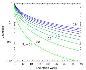
Figure 4: (Color Online) $L(T_{a},\Lambda,I)$ as defined in Eq. (45) versus the Lorentzian width $I$ for $\Lambda=10$ channels and for different values of the transmission coefficient $T_{a}$. From the lowest to the highest curve $T_{a}$ changes from 0.1 to 0.9 in steps of width 0.1.

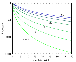
Figure 5: (Color Online) $L(0.5,\Lambda,I)$ as defined in Eq. (45) versus the the Lorentzian width $I$ for $T_{a}=0.5$ and for different channel numbers $\Lambda$. From the lowest to the highest curve the values of $\Lambda$ are 2, 5, 10, 20, 30, 40, and 50.

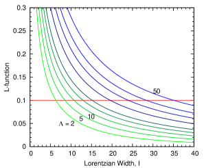
Figure 6: (Color Online) $L(0.99,\Lambda,I)$ as defined in Eq. (45) versus the Lorentzian width $I$ for $T_{a}=0.99$ and for different channel numbers $\Lambda$. From the lowest to the highest curve the values are $\Lambda$ = 2, 3, 4, 5, 6, 8, 10, 12, and 15. The horizontal line shows $L=0.1$.

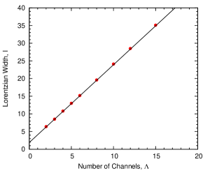
Figure 7: (Color Online) The symbols show for which values of the Lorentzian width $I$ and channel number $\Lambda$ the function $L(0.99,\Lambda,I)$ attains the value $0.1$. The line is a least-squares fit to the symbols; $I(L=0.1)\simeq 2.2\Lambda+1.9.$

IV.2 Asymptotic value at strong-absorption limit

IV.2.1 Elastic enhancement factor in Ericson limit

In the strong-absorption or Ericson limit $\sum_{a}T_{a}\gg 1$, Eq. (35) yields $W_{a}=2$ for the elastic enhancement factor or, equivalently, $\nu_{a}=2$ for the channel degree-of-freedom Verbaarschot86 . Explicitly we have

$$\langle\sigma_{ab}\rangle=\frac{(1+\delta_{ab})T_{a}T_{b}}{\sum_{c}T_{c}}+\ldots\ .$$ (48)

The dots indicate terms of order $(\sum_{c}T_{c})^{-2}$ or higher. The term of leading order is the Hauser-Feshbach result with an elastic enhancement factor of two. Most statistical models agree with that result. An exception is the model by Moldauer, which has an asymptotic value of $\nu_{a}=1.78$. Although Moldauer’s heuristic method to obtain Eq (78) in the Appendix is somewhat similar to the MC technique we adopt here, there is a notable difference between the two approaches. In the MC approach we perform the ensemble average over the elements of the Hamiltonian $H_{\mu\nu}^{({\rm GOE})}$. Moldauer’s statistical $R$-matrix model has two independent inputs: the decay widths drawn from the Porter-Thomas distribution, and the level spacing sampled from the Wigner distribution in Eq. (29).

IV.2.2 Decay amplitude distribution

Our aim is to reproduce Moldauer’s lower asymptotic value by modifying the MC sampling method. Before doing that, we show the distribution of the width amplitudes $\sqrt{\pi}\gamma_{a\sigma}$ when we rewrite our stochastic $S$-matrix of Eq. (31) in an equivalent form Verbaarschot85 ; Mitchel10

$$K_{ab}(E) = \sum_{\sigma}\frac{\tilde{W}_{a\sigma}\tilde{W}_{\sigma b}}{E-E_{\sigma}}\ ,$$ (49)

$$\tilde{W}_{\sigma a} = \sqrt{\pi}\sum_{\nu}{\cal O}_{\sigma\nu}W_{\nu a}\ ,$$ (50)

$${\cal O}^{-1}H^{(\rm GOE)}{\cal O} = \mbox{diag}(E_{\sigma})\ ,$$ (51)

where $E_{\sigma}$ is the eigenvalue of $H^{(\rm GOE)}$. In this form the width amplitudes $\tilde{W}_{a\sigma}=\sqrt{\pi}\gamma_{a\sigma}$ are uncorrelated Gaussian-distributed random variables with zero mean values and the standard deviation. We produced the distributions of $\tilde{W}$ for the case $N=100$, $\Lambda=2$, and three values of $T_{a}=0.1$, 0.5, and 0.99.

The width distributions are shown in Fig. 8 for the elastic channel. Because we used the same transmission for both channels, the distribution for the elastic and inelastic channels are identical. Figure 9 shows the standard deviation $\sigma_{a}$ for each Gaussian for various $T_{a}$.

The second moment of Gaussian distribution is given by Verbaarschot85

$$\sigma_{a}^{2}=\frac{d}{\pi}\frac{T_{a}}{2-T_{a}\pm\sqrt{1-T_{a}}}\ ,$$ (52)

which is shown by the two dashed curves in Fig. 9. The sign ambiguity in Eq. (52) is caused by the fact that there are two values of $\overline{S}_{aa}$ with opposite signs that yield the same value of $T_{a}=1-|\overline{S}_{aa}|^{2}$.

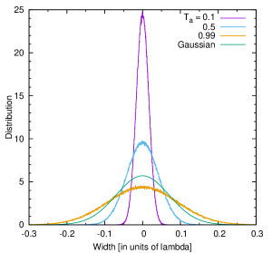
Figure 8: (Color Online) Distribution of decay amplitudes $\gamma_{a\sigma}$, when the GOE $S$ matrix is written in the $K$-matrix form. The histograms correspond to $T_{a}=0.1$, 0.5, and 0.99, respectively. For $T_{a}=0.99$, we compare the Gaussian distribution with the one obtained from the standard deviation in Eq. (59).

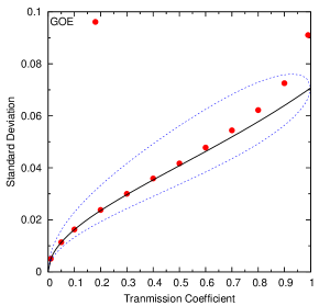
Figure 9: (Color Online) Standard deviation of GOE decay amplitude distribution as a function of transmission coefficient. The dashed curves are Eq. (52) and the solid curve is Eq. (59).

IV.2.3 Emulating Moldauer’s calculation

Moldauer’s $K$ matrix (see Section II.2) can be written as

$$K_{ab}^{\rm M}(E)=\delta_{ab}\Re K_{a}^{0}+\sum_{\sigma}\frac{w_{a\sigma}w_{\sigma b}}{E-E_{\sigma}}\ .$$ (53)

The elements $K_{a}^{0}$ of the elastic background matrix and the variances of the amplitudes $w$ are determined by the energy-averaged $S$ matrix. For $K_{a}^{0}$ we have

$$K^{0}=i\frac{1-S^{(\rm GOE)}(E+iI)}{1+S^{(\rm GOE)}(E+iI)}\ ,$$ (54)

showing that $K_{a}^{0}$ is determined by the transmission coefficient $T_{a}$. Since $\Im S(E+iI)\sim 0$, we may omit the background term $\Re K_{a}^{0}$. When we view the $K$-matrix as an $R$-matrix, $\Im K(E+iI)$ is the pole strength $2\pi\overline{\gamma_{a}^{2}}/d$, therefore the second moment for the distribution of the widths $w_{a\sigma}$ reads

$$\sigma_{a}^{2}=2\pi\overline{\gamma_{a}^{2}}=\frac{d}{\pi}\left|\Im K_{a}^{0}\right|\ .$$ (55)

The elastic enhancement factor $W_{a}$ can be defined only when all channels are identical, $T_{a}=T_{b}=\ldots=T_{\Lambda}$. That is the case we address.

The calculation of the ensemble average of Eq. (53) proceeds as follows. First we generate $S$ of Eq. (31), and convert it into $K$ via Eq. (21). As Moldauer performed in Ref. Moldauer80 , we use $K(E+iI)$ and Eq. (55) to determine the average widths of the decay amplitudes. The latter are then sampled from Gaussians with widths $\sigma_{a}$, independently of the GOE eigenvalues. The Lorentzian average width $I$ is taken to be 0.2 $\lambda$. We extract the elastic enhancement factors and compare with the standard GOE simulation that is described in Sec. III.2.

The elastic enhancement factor $W_{a}$ is calculated as

$$W_{aa} = \frac{\overline{|S_{aa}^{{\rm fl}}|^{2}}}{\sigma_{aa}^{{\rm HF}}}\ ,\qquad\sigma_{aa}^{{\rm HF}}=\frac{T_{a}^{2}}{\Lambda T_{a}}\ ,$$ (56)

$$W_{a} = \frac{(\Lambda-1)W_{aa}}{\Lambda-W_{aa}}\ ,\qquad\nu_{a}=\frac{2}{W_{a}-1}\ .$$ (57)

We calculate $K(E+iI)$ for each realization of the GOE $S$-matrix. Therefore, the ensemble average of Eq. (53) converges slowly. In addition, simulations for very large values of $N$ or $\Lambda$ are not feasible in general. We chose $N=200$, $\Lambda=5$, 10, 20, and 30. The transmission coefficients are 0.25 and 0.75. These combinations roughly cover Moldauer’s numerical study of the strong-absorption cases.

The values of $\nu_{a}$ versus $\sum_{a}T_{a}$ obtained in that way are compared with the GOE result in Fig. 10. The symbols in the upper panel show the results of the standard GOE simulation, those in the lower panel the results of the simulation described in the previous paragraph. The curves in the upper panel represent Eqs. (90), those in the lower panel represent Eq. (78), both for the cases $T_{a}=0.25$ and 0.75. These equations are meant to approximate $\nu_{a}$ for given values of the transmission coefficients. The results of the GOE simulation are well represented by Eq. (90) which has the asymptotic value of 2 in the strong-absorption limit. The MC simulation that uses Eq. (55) tends to give lower $\nu_{a}$ values, similar to Moldauer’s findings.

A plausible explanation of this discrepancy relates to the determination of the decay amplitude via Eq. (55). Since

$$\Im K_{a}^{0}=\frac{T_{a}}{2-T_{a}}\ ,$$ (58)

the widths in Moldauer’s approach have a second moment given by

$$\sigma_{a}^{2}=\frac{d}{\pi}\frac{T_{a}}{2-T_{a}}\ ,$$ (59)

which is shown in Fig. 9 by the solid curve. Comparison with Eq. (52) shows that this is correct only for small values of $T_{a}$. Discrepancies arise for $T_{a}\approx 1$. In Fig 8 we compare for $T_{a}=0.99$ the distribution of widths using for the second moment the correct expression (52) with the one obtained from Moldauer’s equation (59). (We do not show the $T_{a}=0.1$ and 0.5 cases because they perfectly overlap with the exact values). We note that Moldauer’s approach gives a slightly narrower distribution. We suspect that this is the root of Moldauer’s incorrect asymptotic value for $\nu_{a}=1.78$.

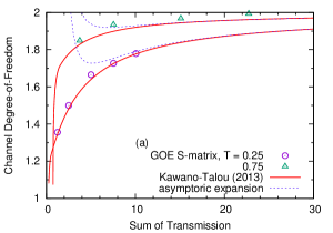
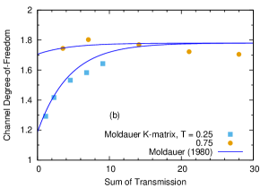
Figure 10: (Color Online) Channel degree-of-freedom values $\nu_{a}$ as functions of $\sum_{a}T_{a}$. The symbols are the Monte-Carlo simulation results, see text. The solid curves in the top panel are from Eq. (88), and the dotted curves are from Eq. (81) for $T_{a}=0.25$ and 0.75. The curves in the bottom panel show Moldauer’s systematics given by Eq. (78) for the same set of $T_{a}$.

IV.2.4 Asymptotic expansion

The next-to-leading-order term of Eq. (48) is given by an asymptotic expansion of Eq. (35) in inverse powers of $\sum_{c}T_{c}$ Weidenmuller84 ; Verbaarschot86 , which is also given in Appendix. This is shown by the dashed curves in Fig. 10 (a). The asymptotic expansion approximates the GOE triple-integral very well, when $\sum_{c}T_{c}>10$. This might be practically useful in the strong-absorption limit, in particular when the number of open channels is so large that calculation of the GOE triple-integral becomes extremely difficult.

IV.3 Very weak entrance channel

An extreme case where all the statistical models fail is reported in Ref. Kawano13 . When there are few open channels with either very small or very large transmission coefficients, none of the width fluctuation models reproduces the GOE results. That was also discussed by Moldauer Moldauer76 as the total width fluctuation, and his numerical study shows a strong enhancement in the elastic channel. We performed the GOE simulation for the case of $N=100$, $\Lambda=2$ and $T_{a}/T_{b}\ll 1$. The calculated width fluctuation correction factor $W_{aa}$, which is the ratio of the elastic channel cross section to the Hauser-Feshbach cross section, is shown in Fig. 11. Since the GOE triple-integral is correct for all values of $\Lambda$ and $T_{a}$, the MC simulation perfectly agrees with GOE, except some deviation seen at very small $T_{a}/T_{b}$ values, due to numerical instability.

Few-channel cases with very different values of the transmission coefficients are very special and hard to realize in practice. A photo-induced reaction that creates a compound nucleus just above neutron threshold could be a case in point. However, since almost all incoming flux goes to the neutron channel and to the other gamma channels, the photon compound elastic cross section is tiny even if it is enhanced by a factor of 50. That is why it might be difficult to confirm the strong enhancement in the elastic channel experimentally.

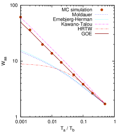
Figure 11: (Color Online) Ratio of the elastic cross section to the Hauser-Feshbach prediction as a function of the ratio $T_{a}/T_{b}$ of transmission coefficients. The symbols are the MC simulation results. The curves are predictions by various statistical models.

V Direct reactions

V.1 Engelbrecht-Weidenmüller transformation

So far it was assumed that the average $S$ matrix is diagonal. That assumption fails when some channels are strongly coupled. In practice that happens, for instance, when collective states in the target nucleus are excited by an incident nucleon (a direct reaction). In such cases, the average $S$ matrix is not diagonal. The unitarity of the scattering matrix imposes strong constraints on the scattering amplitudes. As a consequence, directly coupled channels cause correlations between the resonance amplitudes in those channels. That is why the calculation of the average compound-nucleus cross section in the presence of direct reactions has been a long-standing problem.

When $\langle S\rangle$ is not diagonal, the definition of the transmission coefficients $T$ must be generalized. That is done using Satchler’s transmission matrix Satchler63

$$P_{ab}=\delta_{ab}-\sum_{c}\langle S_{ac}\rangle\langle S_{bc}^{*}\rangle\ .$$ (60)

In the strong-absorption limit, Kawai, Kerman and McVoy (KKM) Kawai73 expressed the compound-nucleus cross section in terms of the matrix $P$ (see Eqs. (79) and (80)). Actual calculations using KKM including the direct channels are, unfortunately, very limited, e.g. Refs.Arbanas08 and Kawano08 .

In practical calculations, an often-used approximate way to include the direct reaction in the statistical model consists in redefining the transmission coefficients so as to take account of some direct reaction contribution,

$$T^{\prime}_{a}=1-\sum_{c}|\langle S_{ac}\rangle\langle S_{ac}\rangle^{*}|^{2}\ .$$ (61)

The sum of the modified transmission coefficients $T^{\prime}_{a}$ equals ${\rm Tr}(P)$. Therefore, it is reasonable to expect that GOE cross-section calculations using the modified transmission coefficients $T^{\prime}_{a}$ as input parameters as done in Ref. Kawano09 may not be far off the mark. In comparison with the exact approach introduced below, the method greatly simplifies the calculations. However, a quantitative validation of the simplification (61) and an understanding of its limitations are still needed.

The following rigorous treatment of the direct reaction was proposed by Engelbrecht and Weidenmüller (EW) Engelbrecht73 . Since $P$ is hermitian, $P$ can be diagonalized by a unitary matrix

$$(UPU^{\dagger})_{ab}=\delta_{ab}p_{a}\ ,\qquad 0\leq p_{a}\leq 1\ .$$ (62)

The transformation $U$ also diagonalizes the average scattering matrix,

$$\langle\tilde{S}\rangle=U\langle S\rangle U^{T}\ {\rm with}\ \langle\tilde{S}\rangle_{ab}=\delta_{ab}\langle\tilde{S}\rangle_{aa}\ .$$ (63)

In the diagonal basis of $P$, the transmission coefficients are given by

$$p_{a}=1-|\langle\tilde{S}_{aa}\rangle|^{2}\ .$$ (64)

In that basis, the decay amplitudes in different channels are statistically uncorrelated, and the calculation of $\overline{\tilde{S}_{pq}\tilde{S}_{rs}^{*}}$ proceeds as described above for the case without direct reactions, with $p_{a}$ as input parameters. The result must be transformed back to the physical channels. That gives Hofmann75

$$\overline{|S_{ab}|^{2}}=\sum_{pqrs}U_{pa}^{*}U_{qb}^{*}U_{ra}U_{sb}\overline{\tilde{S}_{pq}\tilde{S}_{rs}^{*}}\ .$$ (65)

Moldauer demonstrated the impact of the EW transformation numerically Moldauer75b . He argued that the flux into the strongly coupled inelastic channels is enhanced. Capote et al. Capote14 demonstrated that enhancement by applying the coupled-channels code ECIS ECIS to neutron scattering off ²³⁸U. Although ECIS is capable of performing the EW transformation, it has some approximations and limited functionality, particularly for calculating the neutron radiative capture and fission channels. The EW approach uses only the average $S$ matrix as input and facilitates showing how direct reactions impact on the compound nucleus.

A closed form of the average cross section based on the GOE triple-integral formula that takes the EW transformation into account, was derived by Nishioka, Weidenmüller, and Yoshida Nishioka89 . However, the computation might be impractical. We follow the EW transformation step-by-step from Eq. (60) to Eq (65). The result allows us to estimate uncertainties due to the approximation Eq. (61).

V.2 Ensemble average using EW transformation

To implement direct reactions, one may use, for instance, the pole expansion of the $S$ matrix. We find it simpler to employ the $K$-matrix as in Eq. (22). We allow for a direct background by writing

$$K_{ab}(E)=K^{(0)}_{ab}+\sum_{\sigma}\frac{\tilde{W}_{a\sigma}\tilde{W}_{\sigma b}}{E-E_{\sigma}}$$ (66)

where the elements of the background matrix $K^{(0)}$ serve as parameters. When $K$ is real and symmetric, $S$ is automatically unitary.

We consider a case with direct coupling between two channels only. The background matrix $K^{(0)}$ is

$$K^{(0)}=\left(\begin{array}[]{cccc}k_{aa}&k_{ab}&0&\cdots\\ k_{ab}&k_{bb}&0&\cdots\\ 0&0&0&\cdots\\ \vdots&\vdots&\vdots\\ \end{array}\right)\ .$$ (67)

For the sake of simplicity, we take $k_{aa}=k_{ab}=k_{bb}=k_{0}$, where $k_{0}$ is real. The average $S$ matrix is

$$\overline{S}=\frac{1-iK^{(0)}+\pi\langle\tilde{W}_{a}\tilde{W}_{b}\rangle}{1+iK^{(0)}-\pi\langle\tilde{W}_{a}\tilde{W}_{b}\rangle}\ .$$ (68)

The amplitudes $\tilde{W}_{a\sigma}$ are zero-centered Gaussian-distributed random variables, uncorrelated for $a\neq b$. The parameters then are $N,\Lambda,T_{a},k_{0}$. For simplicity we use the same $T_{a}$ for all channels.

The cross sections are calculated in the following three ways.

• For each value of $k_{0}$, the MC method is used to generate 100,000 realizations of $S$. The average cross section is obtained directly as the average of $|\delta_{ab}-S_{ab}|^{2}$ over that ensemble. Figure 12 shows the cross sections for $N=100$, $\Lambda=2$, $T_{a}=0.8=T_{b}$, and for $k_{0}$ varying from 0 to 2 obtained in that way. The top panel shows the elastic scattering cross section $|1-S_{aa}|^{2}$, the bottom panel shows the inelastic scattering cross section $|S_{ab}|^{2}$.

• The average of $S$ over the ensemble of 100,000 realizations is used to calculate the modified transmission coefficients $T^{\prime}_{a}$ of Eq. (61). These are used in the GOE triple-integral to calculate the width fluctuation correction.

• $\overline{S}$ as obtained in the previous step is diagonalized using the EW transformation. The eigenvalues $p_{a}$ are used in the GOE triple-integral. The result $\overline{\tilde{S}_{pq}\tilde{S}_{rs}^{*}}$ is back-transformed to $\overline{|S_{ab}|^{2}}$.

We analyze our results in terms of the usual “optical model” cross sections

$$\sigma_{\rm T} = 2(1-\Re\overline{S}_{aa})\ ,$$ (69)

$$\sigma_{\rm SE} = |1-\overline{S}_{aa}|^{2}\ ,$$ (70)

$$\sigma_{\rm DI} = |\overline{S}_{ab}|^{2}\ .$$ (71)

Here $\sigma_{\rm T}$, $\sigma_{\rm SE}$ and $\sigma_{\rm DI}$ stand for the total, the shape elastic, and the direct inelastic cross section, respectively. The reaction cross section and the compound formation cross section are defined as $\sigma_{\rm R}=\sigma_{\rm T}-\sigma_{\rm SE}$ and $\sigma_{\rm CN}=\sigma_{\rm R}-\sigma_{\rm DI}$, respectively. All these cross sections are given by the coupled-channels optical model, while the compound elastic ($\sigma_{\rm CE}$) and compound inelastic ($\sigma_{\rm CI}$) cross sections require statistical-model calculations. We do not use a coupled-channels optical model in the present context but are able to calculate all these cross sections directly from the MC simulation. The parameter $k_{0}$ controls the strength of $\sigma_{\rm DI}$ up to a limit defined by unitarity — since $\sigma_{\rm T}$ and $\sigma_{\rm SE}$ are connected by $\overline{S}_{aa}$, $\sigma_{\rm R}$ is constrained even if $k_{0}$ is very large.

Figure 13 shows how the compound-inelastic scattering cross section changes with the strength of the direct reaction. We plot the ratio of $\sigma_{\rm CI}$ to the reaction cross section $\sigma_{\rm R}$ as a function of the ratio $\sigma_{\rm DI}/\sigma_{\rm R}$. The upper panel is for $T_{a}=0.5$ and the lower panel is for $T_{a}=0.9$. In each panel we show two cases, $\Lambda=2$ and 10. The results from the EW transformation agree perfectly with the MC simulations, confirming that the EW transformation with the GOE triple-integral yields the correct average cross section when there are strongly coupled channels.

When the background $K$-matrix is parametrized as in Eq. (67), $\sigma_{\rm CI}$ approaches the unitarity limit for very large $k_{0}$. At this limit, we have $\sigma_{\rm CE}\simeq\sigma_{\rm CI}$. The elastic enhancement disappears when a direct channel becomes very strong. Since we employed the same transmission coefficients for all channels, the compound elastic and inelastic scattering cross sections are equal in that limit and given by $\sigma_{\rm CN}/\Lambda$. Use of the modified transmission coefficients $T_{a}^{\prime}$ overestimates $\sigma_{\rm CE}$ and underestimates $\sigma_{\rm CI}$. The discrepancy increases with increasing $\sigma_{\rm DI}$.

The EW transformation is definitely required to calculate the correct compound cross sections when $\Lambda$ is small and $\sigma_{\rm DI}/\sigma_{\rm R}$ is larger than about 5%. A case in point might be a reaction induced by neutrons of several 100 keV impinging on an actinide. Several levels of the ground-state rotational band will be excited by the direct inelastic scattering process. A simple coupled-channels calculation for the 300-keV neutron-induced reaction on ²³⁸U gives $\sigma_{\rm DI}/\sigma_{\rm R}$ of about 0.1. Therefore the approximate method that uses the modified transmission coefficients $T^{\prime}_{a}$ is expected to result in an underestimate of $\sigma_{\rm CI}$.

Figure 12: (Color Online) Simulated elastic (top panel) and inelastic (bottom panel) scattering cross sections as functions of the background parameter $k_{0}$.

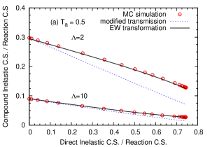
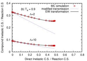
Figure 13: (Color Online) Ratio $\sigma_{\rm CI}/\sigma_{\rm R}$ of the compound inelastic scattering cross section to the reaction cross section as a function of the ratio $\sigma_{\rm DI}/\sigma_{\rm R}$ of direct reaction cross section to the reaction cross section. The symbols show the ensemble average of the MC simulation, the dotted lines are cross sections calculated with the modified transmission coefficients $T^{\prime}_{a}$, and the solid lines are the result of the EW transformation. The top panel is for $T_{a}=0.5$, and the bottom panel is for $T_{a}=0.9$.

VI Conclusion

We have investigated the statistical properties of the scattering matrix containing a GOE Hamiltonian in the propagator. That $S$ matrix describes general chaotic scattering and applies to compound-nuclear reactions at low incident energies (below the precompound regime). We have compared results for average cross sections obtained from Monte-Carlo (MC) simulations with those from the GOE triple integral and from statistical models. The latter give heuristic accounts of the width fluctuation correction. In the GOE approach, the results depend on few parameters: the number $N$ of resonances, the number $\Lambda$ of open channels, and the average $S$ matrix elements. Without direct reactions, the average $S$ matrix is diagonal, and the relevant parameters are the transmission coefficients in the channels. When the channels are strongly coupled and the average $S$ matrix is not diagonal, the number of parameters is correspondingly increased. Our simulations indicate the range of validity of the heuristic models and have led to the following conclusions:

• For all parameter values studied, the numerical average of MC-generated cross sections coincides with the result of the GOE triple-integral formula (35). Although that formula is derived in the limit of a large number of resonances, it gives the correct average even if the number of resonances is small.

• Energy average and ensemble average agree reasonably well (i) for isolated resonances when the width of the Lorentzian averaging function is one or two orders of magnitude larger than the average resonance spacing and (ii) in the Ericson regime when the width of the Lorentzian averaging function is one or two orders of magnitude larger than the average total width of the resonances.

• In the strong-absorption limit (Ericson regime) where $\sum_{a}T_{a}\gg 1$, the channel degree-of-freedom $\nu_{a}$ is 2, different from Moldauer’s asymptotic value of 1.78.

• In extreme cases where a few open channels (including the incident channel) have very small transmission coefficients and a few others have transmission coefficients close to unity, the elastic channel is significantly enhanced. Most of the standard statistical models cannot predict that enhancement. The GOE triple integral is the only way to produce the correct average cross section.

• Direct reactions (for instance, the excitation of states of a rotational band due to inelastic scattering) cause the average $S$ matrix $\overline{S}$ to acquire large off-diagonal elements. Using the Engelbrecht-Weidenmüller (EW) transformation we have diagonalized $\overline{S}$ and evaluated the GOE triple integral in the diagonal channel basis. The results agree with the MC simulations. We find that the direct reaction increases the inelastic cross sections while the elastic cross section is reduced.

*

Appendix A Statistical models

A.1 HRTW

In the HRTW approach Hofmann75 ; Hofmann80 , an elastic enhancement factor $W_{a}$ is expressed by the channel transmission coefficient $T_{a}$, and all the channel cross sections are calculated from an effective transmission coefficient $V_{a}$

$$\langle\sigma_{ab}\rangle=\frac{V_{a}V_{b}}{\sum_{c}V_{c}}\left\{1+\delta_{ab}(W_{a}-1)\right\}\ ,$$ (72)

where $V_{c}$’s are determined from the unitarity of $S$-matrix, in another word, the flux conservation. The values of $W_{a}$ were derived from the statistical $K$-matrix analysis. There are two sets of $W_{a}$ parameterization, namely in the original paper of Ref. Hofmann75 , and the updated parameters in Ref. Hofmann80 . We refer to the updated parameters as HRTW, which reads

$$W_{a} = 1+\frac{2}{1+T_{a}^{F}}+87\left(\frac{T_{a}-\overline{T}}{T}\right)^{2}\left(\frac{T_{a}}{T}\right)^{5}\ ,$$ (73)

$$F = 4\frac{\overline{T}}{T}\left(1+\frac{T_{a}}{T}\right)\left(1+3\frac{\overline{T}}{T}\right)^{-1}\ ,$$ (74)

where $\overline{T}$ is the average value of $T_{a}$, and $T$ is the sum of $T_{a}$ for the all open channels $T=\sum_{c}T_{c}$.

A.2 Moldauer

The Gaussian distribution of $\gamma_{\mu a}$ yields the Porter-Thomas distribution of $\gamma_{\mu a}^{2}$ when there is only one channel. More generally, the distribution of $\gamma_{\mu a}^{2}$ will be the $\chi^{2}$ distribution with the channel degree-of-freedom $\nu_{a}$. In these circumstances, the width fluctuation correction factor can be evaluated numerically as Moldauer75a ; Moldauer75b ; Moldauer76

$$W_{ab} = (1+\frac{2\delta_{ab}}{\nu_{a}})\int_{0}^{\infty}\!\!\!\frac{dt}{F_{a}(t)F_{b}(t)\Pi_{k}F_{k}(t)^{\nu_{k}/2}},$$ (75)

$$F_{k}(t) = 1+\frac{2}{\nu_{k}}\frac{T_{k}}{T}t\ .$$ (76)

The integration can be performed easily by changing the variable $t$ into $z$ as

$$t=\frac{z}{1-z},\qquad\frac{dt}{dz}=\frac{1}{(1-z)^{2}}\ ,$$ (77)

where $z\rightarrow 0$ for $t=0$, and $z\rightarrow 1$ for $t\rightarrow\infty$.

In contrast to HRTW, Moldauer’s prescription gives the width fluctuation correction factor that ensures the unitarity for all the channels when the channel degree-of-freedom $\nu_{a}$ is provided. Moldauer obtained $\nu_{a}$ as a function of each channel transmission coefficient $T_{a}$ and the sum of them $T=\sum_{c}T_{c}$ with the MC simulation, which reads Moldauer80

$$\nu_{a}=1.78+(T_{a}^{1.212}-0.78)\exp(-0.228T)\ .$$ (78)

The channel degree-of-freedom $\nu_{a}$ is related to the elastic enhancement factor $W_{a}=1+2/\nu_{a}$.

A.3 KKM

The model of Kawai, Kerman, McVoy Kawai73 is very different from the MC approach of HRTW or Moldauer. The $S$-matrix is expressed in terms of the optical $S$-matrix background, in which the energy average of the resonance sum part will be zero. The optical model (or the coupled-channels optical model) yields Satchler’s transmission matrix Satchler63 , and a new hermitian matrix $X$ in channel space is defined as

$$X=-\frac{1}{2}{\rm tr}X+\left\{({\rm tr}X/2)^{2}+P\right\}^{1/2}\ .$$ (79)

In the overlapping resonance limit ($\Gamma/D\gg 1$), the average cross section is written in terms of the $X$-matrix as

$$\langle\sigma_{ab}\rangle=X_{aa}X_{bb}+X_{ab}X_{ba}\ .$$ (80)

Since Eq. (79) is a non-linear equation in $X$, one has to solve it by an iterative procedure Kawano08 . When $\langle S\rangle$ is diagonal (no direct channel), KKM yields an elastic enhancement factor $W_{a}=2$. In other words, KKM gives the correct asymptotic value in the Ericson regime. That same statement applies in the case of direct reactions. This is seen using the EW transformation.

A.4 GOE

The analytical expression of the correct Hauser-Feshbach cross section, i.e. an analytical average over the GOE resonance parameter distributions, was given by Verbaarschot, Weidenmüller, and Zirnbauer Verbaarschot85 , which is the so-called triple-integral of Eq. (35). The result includes the elastic enhancement and the width fluctuation correction at the same time, which is one of the reasons we defined the width fluctuation correction factor by Eq. (7), namely the cross section ratio to the Hauser-Feshbach formula.

A.5 Asymptotic expansion

An asymptotic expansion of the GOE triple-integral formula in powers of $1/T$ is given by Weidenmuller84

$$\langle\sigma_{ab}\rangle\simeq(1+\delta_{ab})\frac{T_{a}T_{b}}{T}A+2\delta_{ab}\frac{T_{a}^{2}}{T^{2}}B,$$ (81)

where

$$A = 1+\frac{1}{T}\left(1+\frac{2}{T}\right)\left\{\Sigma_{2}-(T_{a}+T_{b})\right\}$$ (82)

$$+ \frac{5}{T^{2}}\Sigma_{2}\left\{\Sigma_{2}-(T_{a}+T_{b})\right\}$$

$$+ \frac{4}{T^{2}}\left(T_{a}^{2}+T_{a}T_{b}+T_{b}^{2}-\Sigma_{3}\right),$$

$$B = (1-T_{a})\left\{1-\frac{2}{T}(1+2T_{a})+\frac{3}{T}\Sigma_{2}\right\},$$ (83)

and

$$\Sigma_{2}=\frac{1}{T}\sum_{c}T_{c}^{2},\qquad\Sigma_{3}=\frac{1}{T}\sum_{c}T_{c}^{3}.$$ (84)

A.6 Ernebjerg and Herman

Ernebjerg and Herman Ernebjerg04 generated a quasi-random set of transmission coefficients, and compared the simulated cross sections with Eqs. (72), (75), and (35). They obtained a new parameterization of the channel degree-of-freedom

$$\nu_{a}=\frac{1}{1+f(T_{a})T^{g(T_{a})}}\ ,$$ (85)

where

$$f(T_{a}) = \frac{0.177}{1-20.337T_{a}}\ ,$$ (86)

$$g(T_{a}) = 1+3.148T_{a}(1-T_{a})\ .$$ (87)

A.7 Kawano and Talou

Similar to Ernebjerg and Herman’s attempt, the GOE triple-integral calculation can be well-approximated by putting the following channel degree-of-freedom in Moldauer’s method

$$\nu_{a}=2-\frac{1}{1+f}\ ,\qquad f=\alpha\beta_{1}\frac{T_{a}+T}{1-T_{a}}\ .$$ (88)

They obtained

$$\alpha = 0.0288T_{a}+0.246\ ,$$ (89)

$$\beta_{1} = 1+2.5T_{a}(1-T_{a})\exp(-2T)\ .$$ (90)

In the special case of $T<2T_{a}$, a better fit can be obtained with

$$f = 3\alpha\beta_{2}x_{a}\left(\frac{T-T_{a}}{T_{a}}\right)^{q}\ ,$$ (91)

$$\beta_{2} = 1+2.5T_{a}(1-T_{a})\exp(-4T)\ ,$$ (92)

where $q=0.4x_{a}^{0.4}$ and $x_{a}=T_{a}/(1-T_{a})$.

References

- (1) N. Bohr, Nature 137, 344 (1936).
- (2) W. Hauser, H. Feshbach, Phys. Rev. 87, 366 (1952).
- (3) A. M. Lane, J. E. Lynn, Proc. Phys. Soc. A 70, 557 (1957).
- (4) P. A. Moldauer, Phys. Rev. C 11, 426 (1975).
- (5) P. A. Moldauer, Phys. Rev. C 12, 744 (1975).
- (6) M. Kawai, A. K. Kerman, K. W. McVoy, Ann. Phys. 75, 156 (1973).
- (7) D. Agassi, H. A. Weidenmüller, G. Mantzouranis, Phys. Rep. 22, 145 (1975).
- (8) H. M. Hofmann, J. Richert, J. W. Tepel, H. A. Weidenmüller, Ann. Phys. 90, 403 (1975).
- (9) P. A. Mello, Phys. Lett. B81, 103 (1979).
- (10) P. A. Mello, T. H. Seligman, Nucl. Phys. A 344, 489 (1980).
- (11) H. M. Hofmann, T. Mertelmeier, M. Herman, J. W. Tepel, Z. Phys. A 297, 153 (1980).
- (12) P. A. Moldauer, “Statistical Theory of Neutron Nuclear Reactions,” ANL/NDM-40, Argonne National Laboratory (1978).
- (13) P. A. Moldauer, Nucl. Phys. A, 344, 185 (1980).
- (14) T. A. Brody, J. Flores, J. B. French, P. A. Mello, A. Pandey, S. S. M. Wong, Rev. Mod. Phys. 53, 385 (1981).
- (15) J. J. M. Verbaarschot, H. A. Weidenmüller, M. R. Zirnbauer, Phys. Rep. 129, 367 (1985).
- (16) C. Mahaux, H. A. Weidenmüller, “Shell-Model Approach to Nuclear Reactions,” North-Holland, Amsterdam, London (1969).
- (17) H. A. Weidenmüller, G. E. Mitchell, Rev. Mod. Phys. 81, 539 (2009).
- (18) G. E. Mitchell, A. Richter, H. A. Weidenmüller, Rev. Mod. Phys. 82, 2845 (2010).
- (19) F. H. Fröhner, Nucl. Sci. Eng. 103, 119 (1989).
- (20) S. Igarasi, “On application of the S-matrix two-point function to nuclear data evaluation,” Proc. Int. Conf. on Nuclear Data for Science and Technology, 13 – 17 May, 1991, Jülich, Germany, Ed. S.M. Qaim, Springer-Verlag, p.903 (1992).
- (21) S. Hilaire, Ch. Lagrange, A. J. Koning, Ann. Phys. 306, 209 (2003).
- (22) M. Ernebjerg, M. Herman, Proc. Int. Conf. on Nuclear Data for Science and Technology, 26 Sept. – 1 Oct., 2004, Santa Fe, USA, Ed. R.C. Haight, M.B. Chadwick, T. Kawano, and P. Talou, American Institute of Physics, AIP Conference Proceedings 769, p.1233 (2005).
- (23) T. Kawano, P. Talou, Nuclear Data Sheets 118, 183 (2014).
- (24) P. A. Moldauer, Phys. Rev. 123, 968 (1961).
- (25) P. A. Moldauer, Phys. Rev. 135, B642 (1964).
- (26) E. P. Wigner, L. Eisenbud, Phys. Rev. 72, 29 (1947).
- (27) M. L. Mehta, “Random Matrices, Third Edition,” Elsevier, Amsterdam (2004).
- (28) F. H. Fröhner, “Evaluation and Analysis of Nuclear Resonance Data,” JEFF Report 18, OECD Nuclear Energy Agency (2000).
- (29) M. B. Chadwick, M. Herman, P. Obložinský, M.E. Dunn, Y. Danon, A.C. Kahler, D.L. Smith, B. Pritychenko, G. Arbanas, R. Arcilla, R. Brewer, D.A. Brown, R. Capote, A.D. Carlson, Y.S. Cho, H. Derrien, K. Guber, G.M. Hale, S. Hoblit, S. Holloway, T.D. Johnson, T. Kawano, B.C. Kiedrowski, H. Kim, S. Kunieda, N.M. Larson, L. Leal, J.P. Lestone, R.C. Little, E.A. McCutchan, R.E. MacFarlane, M. MacInnes, C.M. Mattoon, R.D. McKnight, S.F. Mughabghab, G.P.A. Nobre, G. Palmiotti, A. Palumbo, M.T. Pigni, V.G. Pronyaev, R.O. Sayer, A.A. Sonzogni, N.C. Summers, P. Talou, I.J. Thompson, A. Trkov, R.L. Vogt, S.C. van der Marck, A. Wallner, M.C. White, D. Wiarda, P.G. Young Nuclear Data Sheets 112, 2887 (2011).
- (30) T. Kawano, F. H. Fröhner, Nucl. Sci. Eng. 127, 130 (1997).
- (31) A. Gilbert, A. G. W. Cameron, Can. J. Phys. 43, 1446 (1965).
- (32) T. Kawano, S. Chiba, H. Koura, J. Nucl. Sci. Technol. 43, 1 (2006); T. Kawano, “updated parameters based on RIPL-3,” (unpublished, 2009).
- (33) J. J. M. Verbaarschot, Ann. Phys. 168, 368 (1986).
- (34) H. A. Weidenmüller, Ann. Phys. 158, 120 (1984).
- (35) P. A. Moldauer, Phys. Rev. C 14, 764 (1976).
- (36) G. R. Satchler, Phys. Lett. 7, 55 (1963).
- (37) G. Arbanas, C. Bertulani, D. J. Dean, A. K. Kerman, “Statistical properties of Kawai-Kerman-McVoy T-matrix,” Proc. of the 2007 Int. Workshop on Compound-Nuclear Reactions and Related Topics (CNR* 2007), Tenaya Lodge at Yosemite National Park, Fish Camp, California, USA 22-26 October 2007, AIP Conference Proceedings 1005, pp.160–163 Eds. J. Escher, F.S. Dietrich, T. Kawano, I. Thompson (2008).
- (38) T. Kawano, L. Bonneau, A. Kerman, “Effects of direct reaction coupling in compound reactions,” Proc. Int. Conf. on Nuclear Data for Science and Technology, 22 – 27 Apr., 2007, Nice, France, Ed. O. Bersillon, F. Gunsing, E. Bauge, R. Jacqmin, and S. Leray, EDP Sciences, pp.147–150 (2008).
- (39) T. Kawano, P. Talou, J. E. Lynn, M. B. Chadwick, D. G. Madland, Phys. Rev. C 80, 024611 (2009).
- (40) C. A. Engelbrecht, H. A. Weidenmüller, Phys. Rev. C 8, 859 (1973).
- (41) R. Capote, A. Trkov, M. Sin, M. Herman, A. Daskalakis, Y. Danon, Nucl. Data Sheets 118, 26 (2014).
- (42) J. Raynal, computer code ECIS [unpublished].
- (43) H. Nishioka, H.A. Weidenmüller, S. Yoshida, Ann. Phys. 193, 195 (1989).
*