Using a Power Law Distribution to describe Big Data

Abstract

The gap between data production and user ability to access, compute and produce meaningful results calls for tools that address the challenges associated with big data volume, velocity and variety. One of the key hurdles is the inability to methodically remove expected or uninteresting elements from large data sets. This difficulty often wastes valuable researcher and computational time by expending resources on uninteresting parts of data. Social sensors, or sensors which produce data based on human activity, such as Wikipedia, Twitter, and Facebook have an underlying structure which can be thought of as having a Power Law distribution. Such a distribution implies that few nodes generate large amounts of data. In this article, we propose a technique to take an arbitrary dataset and compute a power law distributed background model that bases its parameters on observed statistics. This model can be used to determine the suitability of using a power law or automatically identify high degree nodes for filtering and can be scaled to work with big data.

Index Terms—  Big Data, Signal Processing, Power Law

1 Introduction

The 3 V’s of big data: volume, velocity and variety [1], provide a guide to the outstanding challenges associated with working with big data systems. Big data volume stresses the storage, memory and compute capacity of a computing system and requires access to a computing cloud. The velocity of big data stresses the rate at which data can be absorbed and meaningful answers produced. Big data variety makes it difficult to develop algorithms and tools that can address the large diversity of input data. One of the key challenges is in developing algorithms that can provide analysts with basic knowledge about their dataset when they have little to no knowledge of the data itself.

In [2], we proposed a series of steps that an analyst should take in analyzing an unknown dataset including a technique similar to spectral analysis - Dimensional Data Analysis (DDA). As a next step in the data analysis pipeline, we propose determining a suitable background model. Big data sets come from a variety of sources such as social media, health care records, and deployed sensors, and the background model for such datasets are as varied as the data itself. One of the popular statistical distributions used to explain such data is the power law distribution. There is much related work in the area. Studies such as  [3, 4, 5, 6] have looked at power laws as underlying models for human generated big data collected from sources such as social media, network activity and census data. However, there has also been some controversy that while data may look like it follows a power law it may in fact be better described by other distributions such as exponential or log-normal distributions [7, 8]. While a power law distribution may seem a fitting background model for an observed dataset, large fluctuations in lower degree terms (the tail of the distribution) may skew the estimation of power law parameters [9]. Further, the estimation of power law exponent can be heavily dependent on decisions such as binning [10] which may lead to problems such as estimator bias [11].

We propose a technique that takes an unknown dataset, estimates the parameters and binning of the degree distribution of an power law distributed dataset that follows constraints enforced by the observed dataset, and aligns the degree distribution of the observed dataset to the structure of the perfect power law distribution in order to provide a clear view into the applicability of a power law model.

The article is structured as follows: Section 2 describes the relationship between signal processing and big data; Section 3 describes the proposed technique to estimate the power law parameters of a dataset; Section 4 describes application examples. Finally, we conclude in Section 5.

2 Signal Processing and Big Data

Detection theory in signal processing is the ability to discern between different signals based on the statistical properties of the signals. In the simplest form, the decision is to choose whether a signal is present or absent. In making this determination, the observed signal is compared against the expected background signal when no signal is present. A deviation from this background model indicates the presence of a signal. While it is common to represent the background model as additive white gaussian noise (AWGN), the model may change depending on physical factors such as channel parameters or known noise characteristics.

Big data can be as a considered a high dimensional signal that is projected to an n-dimensional space. Big data, similar to the 1-, 2- and 3-D signals that signal processing has traditionally dealt with, are often noisy, corrupted, or misaligned. The concept of noise in big data can be thought of as unwanted information which impairs the detection of activity or important entities present in the dataset. For example, consider a situation in which network logs are collected to determine foreign or dangerous connections out of a network. Detecting such activity may be difficult due to the presence of few vertices (such as connections to www.google.com) with a very large number of connections (edges). This information can be considered the equivalent of stop words in text analytics [12, 13]. While such data may help form a useful statistic, often, these entries impair the ability to find activity of interest that occurs at a lower activity threshold. Often, such vertices with a large number of edges (high degree vertices) are manually removed based on empirical evidence in order to improve the big data signal to noise ratio. Knowledge of a suitable big data background model can highlight such vertices and help with the automated removal of components in the dataset which are of minimal interest. This concept parallels the concept of filtering in signal processing. In fact, such parallels between big data and signal processing kernels are numerous. In [14], for example, the authors look at the commonality between certain signal processing kernels and graph operations. As another example, the authors of  [15] study data collected from social networks and their underlying statistical distribution.

Fig. 1: Computing the histogram and degree distribution of 10,000 data points in which the magnitude was determine by drawing from a power law distribution with $\alpha=1.8$.

A common distribution that is observed in many datasets is the power law distribution. A power law distribution is one in which a small number of vertices are incident to a large number of edges. This principle has also been referred to as the Pareto principle, Zepf’s Law, or the 80-20 rule. A power law distribution for a random variable x, is defined to be:

$$p(x)=cx^{-\alpha}$$

where the exponent $\alpha$ represents with the power of the distribution. An illustrative example of 10,000 randomly generated points drawn from a power law distribution with exponent $\alpha=1.8$ is shown in Figure 1. The middle figure shows the histogram of such a random variable. Finally, the rightmost image shows the degree distribution of the signal. Note the large number of low degree nodes and small number of high degree nodes. While a power law distribution may be applicable to a given dataset based on physical characteristics or empirical evidence, a more rigorous approach is needed to fit observed data to a power law model in order to verify the applicability of a power law distribution.

3 Power Law Modeling Technique

This section describes the proposed technique for comparing an observed dataset with an ideal power law distributed dataset whose parameters are derived from a statistical analysis of the observed dataset.

3.1 Definitions

A large dataset can be represented by a graph through the adjacency matrix representation or incidence matrix representation [16]. An adjacency matrix has dimensions $n\times n$, where $n$ corresponds to the number of vertices in the graph. A vertex out-degree is a count of the number of edges in a directed graph which leave a particular vertex. The vertex in-degree, on the contrary, is a count of the number of edges in a directed graph which enter a particular vertex. A popular way to represent the in-degree and out-degree distributions is through the degree distribution which is a statistic that computes the number of vertices that are of a certain degree. Such a count is very relevant to techniques such as graph algorithms and social networks.

The in-degree and out-degree of a graph can be determined by the following relations:

$$d_{in}(i)=\sum_{j}E_{ij}$$

$$d_{out}(i)=\sum_{j}E_{ji}$$

where $d_{in}(i)$ and $d_{out}(i)$ represent the in and out degree at bin $i$ and $E$ represents the graph incidence matrix. The selection of the the total number of bins ($N_{d}$) is an important factor in determining the degree distribution given by $d_{in}$, $d_{out}$, and $i\leq N_{d}$. An illustrative example is shown in Figure 2 to demonstrate the parameters described in this section.

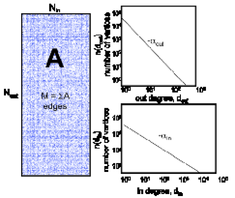
Fig. 2: Adjacency matrix for notional power law distributed random graph with corresponding in and out degree distributions.

The degree distribution conveys many important pieces of information. For example, it may show that a large number of vertices have a degree of 1, which implies that a majority of vertices are connected only to one other vertex. Further, it may show that there are a small number of vertices with high degree (many edges). In a social media dataset, such vertices may correspond to popular users or items.

The maximum degree vertex is said to be $d_{N_{d}}=d_{max}$. The total number of vertices ($N$) and edges ($M$) can be computed as:

$$N=\sum_{i=1}^{N_{d}}n(d_{i})$$

$$M=\sum_{i}^{N_{d}}n(d_{i})*d_{i}$$

where $n(d_{i})$ is defined as number (count) of vertices with degree $d_{i}$.

3.2 Power Law Fitting

Step 1: Find parameters of observed data

In order to determine the power law parameters for an arbitrary data set, data is first converted to an adjacency matrix representation. In the adjacency matrix, row and columns represent vertices with outbound and inbound edges respectively. A non-zero entry at a particular row and column pair indicates the existence of an edge between two vertices. Often, data may be collected and stored in an incidence matrix where rows of the matrix represent edges and columns represent vertices. For data in an intermediate format such as the incidence matrix ($E$), it is possible to convert this representation to the adjacency matrix ($A$) using the following relation:

$$A=|E<0|^{T}*|E>0|$$

where $|E<0|$ and $|E>0|$ represent the incidence matrix with outbound and inbound edges only. From the adjacency matrix, it is possible to calculate the degree distribution as described to extract the parameters $\alpha$, the vertex with maximum degree $d_{max}$, the number of vertices with exactly 1 edge, $n(d_{1})$, and the number of bins $N_{d}$. There are many proposed methods to calculate the power law exponent  [17, 10]. For the purpose of this study, a simple first order estimate of $\alpha$ is sufficient and it should satisfy the intuitive property that the count $n(d_{1})$ and degree $d_{max}$ be included since most natural datasets will have at least one vertex with $degree=1$ and a vertex with large degree. Furthermore, the exponent should take into account. Therefore, we propose the following simple relationship to calculate $\alpha$:

$$\alpha=log(n(d_{1}))/log(d_{max})$$ (1)

Using the power law exponent calculated in Equation 1 allows an initial comparison between the observed dataset and a power law distribution.

Step 2: Calculate “Perfect” Power Law Parameters

Given the degree distribution of the observed data we can compute the parameters: $\alpha^{obs}$, $d_{i}^{obs}$, $n(d_{i}^{obs})$, $N^{obs}_{d}$, $M^{obs}$, and $N^{obs}$, using the relations provided in the definitions section (Section 3.1). In order to see if the observed data fits a power law distribution, we need to be able to determine what an ideal power law distributed dataset would look like for parameters similar to those observed. This ideal distribution is referred to as a “perfect” power law distribution.

The “perfect” power law distribution can be determined by computing the parameters $d_{i}$, $n(d_{i})$, and $N_{d}$ which closely fit the observed data while also maintaining the number of vertices and edges. While theoretically, any distribution which satisfies the properties $\alpha>0$, $d_{max}>1$ and $N_{d}>1$ can be used to form a power law model, we also desire values which maintain the total number of vertices and edges, $N$ and $M$. Essentially, given an observed number of vertices and edges, compute the quantities $N_{d}$, $n(d_{i})$ and $d_{i}$ where $i\leq N_{d}$ that form a power law distribution (with $\alpha$) which also satisfy the property that $M\approx M^{obs}$ and $N\approx N^{obs}$.

These values can be solved by using a combination of optimization techniques such as exhaustive search, simulated annealing, or Broyden’s algorithm, to find the values $d_{i}$ and $n(d_{i})$ that minimize:

$$\min_{d,n}f(d_{i},n(d_{i}))\\ =\sqrt{\arrowvert M^{obs}-\sum_{i}n(d_{i})\arrowvert^{2}+\arrowvert N^{obs}-\sum_{i}n(d_{i})*d_{i}\arrowvert^{2}}$$ (2)

where $M^{obs}$ and $N^{obs}$ are the observed number of edges and vertices. From the estimate of $d_{i}$ and $n(d_{i})$ we can determine $N_{d}$ (given by the number of output $d_{i}$), and $d_{max}$ (given by $d_{N_{d}}$).

Step 3: Align observed data with background model

The values of $N_{d}$, $d_{i}$, and $n(d_{i})$ from the previous step, provides a power law distributed dataset with power $\alpha$. However, the degree binning may be different from the observed distribution. In order to compare the observed data with the background model, it is necessary to rebin the observed data such that it aligns with the background model. Using the rebinned observed data (represented by the parameters $d_{i}^{rebin}$ and $n(d_{i}^{rebin})$) it is possible to determine the power law nature of the observed dataset. Both datasets use the same degree binning using algorithm 1.

Data: $d_{i}$, $d_{i}^{obs}$

Result: $d_{i}^{rebin}$, $n(d_{i}^{rebin})$

for i=1:$N_{d}$ do

      $d_{i}^{rebin}=d_{i}$

      $n(d_{i}^{rebin})$ = number of vertices binned to $i$

end for

Algorithm 1 Algorithm to rebin observed data into fitted data bins

4 Application Example

To demonstrate the application of steps provided in Section  3.2, we describe two examples - a Twitter dataset and a corpus of news articles provided by Reuters. We use the open source Dynamic Distributed Dimensional Data Model (D4M, d4m.mit.edu) to store and access the required data. As a first step, data is converted to the D4M schema  [18], which organizes data into an associative array, representing data as an incidence matrix. The Twitter dataset contains all the metadata associated with approximately 2 million tweets. For the purpose of this example, we have considered only a subset of the data which corresponds to Twitter usernames.

To begin, we determine the adjacency matrix of the associative array data using the relation outlined in the previous section. With the adjacency matrix, we can determine the degree distribution of the observed dataset as demonstrated by the blue circles in Figure 3. Using the values of N and M from this distribution, we can find the values of $d_{i}$ and $n(d_{i})$ that fit the N and M values of the observed dataset. The obtained values are plotted in Figure 3 as the black triangles. As a final step, we rebin the original degree distribution to align with the bins of the ideal distribution. The results of rebinning the observed distribution are shown in Figure 3 as red plus signs.

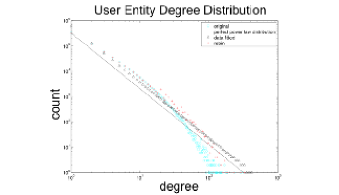
Fig. 3: Fitting a Power Law distribution to Twitter user data.

For the Twitter user data of Figure 3, we see that a power law distribution provides a good representation of the data. The second dataset, a corpus of news articles from Reuters, seems to follow a power law distribution. However, once we fit the perfect power law distribution and rebin the original data, we see that the dataset does not follow a power law distributions evidenced by the large bulge in Figure 4.

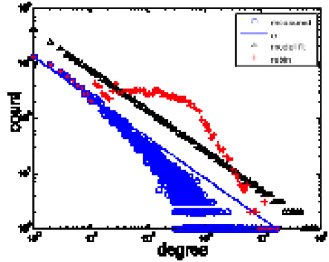
Fig. 4: Fitting a Power Law distribution to Reuters data corpus.

5 Conclusions and Future Work

In this article, we presented a technique to uncover the underlying distribution of a big dataset. One of the most common statistical distributions attributed to a variety of human generated big data sources, such as social media, is the power law distribution. Often, however, data that seems to adhere to a power law distribution may not be well described by such a distribution. In such situations, it is important to be aware of the underlying background model of the dataset before further processing. Our future work includes investigating the big data equivalents of sampling and big data filtering.

6 Acknowledgements

The authors wish to thank the LLGrid team at MIT Lincoln Laboratory for their assisstance in setting up the experiments.

References

- [1] Doug Laney, “3D data management: Controlling data volume, velocity and variety,” META Group Research Note, vol. 6, 2001.
- [2] Vijay Gadepally and Jeremy Kepner, “Big data dimensional analysis,” IEEE High Performance Extreme Computing (HPEC), 2014.
- [3] Mark Newman, “Power laws, pareto distributions and zipf’s law,” Contemporary Physics, vol. 46, no. 5, pp. 323–351, 2005.
- [4] Xavier Gabaix, “Zipf’s law for cities: an explanation,” Quarterly Journal of Economics, pp. 739–767, 1999.
- [5] Lada Adamic and Bernardo Huberman, “Zipf’s law and the internet,” Glottometrics, vol. 3, no. 1, pp. 143–150, 2002.
- [6] Paul Krugman, “The power law of twitter,” http://krugman.blogs.nytimes.com/2012/02/08/the-power-law-of-twitter/?_php=true&_type=blogs&_r=0, 2014.
- [7] Michael Mitzenmacher, “A brief history of generative models for power law and lognormal distributions,” Internet mathematics, vol. 1, no. 2, pp. 226–251, 2004.
- [8] “Twitter followers do not obey a power law, or paul krugman is wrong,” http://blog.luminoso.com/2012/02/09/twitter-followers-do-not-obey-a-power-law-or-paul-krugman-is-wrong/.
- [9] Aaron Clauset, Cosma Rohilla Shalizi, and Mark Newman, “Power-law distributions in empirical data,” SIAM review, vol. 51, no. 4, pp. 661–703, 2009.
- [10] Ethan White, Brian Enquist, and Jessica Green, “On estimating the exponent of power-law frequency distributions,” Ecology, vol. 89, no. 4, pp. 905–912, 2008.
- [11] Michel L. Goldstein, Steven A. Morris, and Gary G. Yen, “Problems with fitting to the power-law distribution,” The European Physical Journal B-Condensed Matter and Complex Systems, vol. 41, no. 2, pp. 255–258, 2004.
- [12] Wayne Xin Zhao, Jing Jiang, Jianshu Weng, Jing He, Ee-Peng Lim, Hongfei Yan, and Xiaoming Li, “Comparing twitter and traditional media using topic models,” in Advances in Information Retrieval, pp. 338–349. Springer, 2011.
- [13] Efthymios Kouloumpis, Theresa Wilson, and Johanna Moore, “Twitter sentiment analysis: The good the bad and the omg!,” Icwsm, vol. 11, pp. 538–541, 2011.
- [14] Aliaksei Sandryhaila and Jose Moura, “Big data analysis with signal processing on graphs: Representation and processing of massive data sets with irregular structure,” Signal Processing Magazine, IEEE, vol. 31, no. 5, pp. 80–90, 2014.
- [15] Lev Muchnik, Sen Pei, Lucas C. Parra, Saulo D. S. Reis, José. Andrade Jr, Shlomo Havlin, and Hernán A. Makse, “Origins of power-law degree distribution in the heterogeneity of human activity in social networks,” Nature Scientific Reports, vol. 3, 05 2013.
- [16] Delbert Fulkerson and Oliver Gross, “Incidence matrices and interval graphs,” Pacific journal of mathematics, vol. 15, no. 3, pp. 835–855, 1965.
- [17] Heiko Bauke, “Parameter estimation for power-law distributions by maximum likelihood methods,” The European Physical Journal B-Condensed Matter and Complex Systems, vol. 58, no. 2, pp. 167–173, 2007.
- [18] Jeremy Kepner, Christian Anderson, William Arcand, David Bestor, Bill Bergeron, Chansup Byun, Matthew Hubbell, Peter Michaleas, Julie Mullen, David O’Gwynn, et al., “D4M 2.0 schema: A general purpose high performance schema for the accumulo database,” in IEEE High Performance Extreme Computing Conference (HPEC), 2013.