Connecting massive galaxies to dark matter halos in BOSS - I. Is galaxy color a stochastic process in high-mass halos?
Abstract
We use subhalo abundance matching (SHAM) to model the stellar mass function (SMF) and clustering of the Baryon Oscillation Spectroscopic Survey (BOSS) “CMASS” sample at . We introduce a novel method which accounts for the stellar mass incompleteness of CMASS as a function of redshift, and produce CMASS mock catalogs which include selection effects, reproduce the overall SMF, the projected two-point correlation function , the CMASS , and are made publicly available. We study the effects of assembly bias above collapse mass in the context of “age matching” and show that these effects are markedly different compared to the ones explored by Hearin et al. (2013) at lower stellar masses. We construct two models, one in which galaxy color is stochastic (“AbM” model) as well as a model which contains assembly bias effects (“AgM” model). By confronting the redshift dependent clustering of CMASS with the predictions from our model, we argue that that galaxy colors are not a stochastic process in high-mass halos. Our results suggest that the colors of galaxies in high-mass halos are determined by other halo properties besides halo peak velocity and that assembly bias effects play an important role in determining the clustering properties of this sample.
keywords:
cosmology: large-scale structure of Universe, cosmological parameters, galaxies: halos, statistics1 Introduction
The overall picture that galaxies form, evolve, and reside in dark matter halos that assemble hierarchically has gained consensus by passing a variety of observational tests over a wide range of cosmic history (for a review, see Mo et al., 2010). However, understanding the detailed relation between galaxies and dark matter halos is critical in order to form a more concrete theory of galaxy formation and evolution. In particular, unveiling how the stellar masses and star-formation properties of galaxies depend on halo properties is still a topic of active investigation. For low-mass galaxies (), recent studies of galaxy clustering and galaxy-galaxy lensing suggest that red and blue galaxies live in halos of different mass at fixed stellar mass at (Zehavi et al., 2005; Mandelbaum et al., 2006; Tinker et al., 2013; Coupon et al., 2015; Mandelbaum et al., 2015) or that at fixed stellar mass, galaxy color may correlate with halo age (Hearin et al., 2014b).
While many previous studies focus on low or intermediate mass galaxies, the galaxy-halo mass connection is also worth investigating for the most massive galaxies in the universe. The majority of galaxies with masses are centrals hosted by massive halos () (White et al., 2011; Leauthaud et al., 2011; Coupon et al., 2015). From a theoretical standpoint, gas in these high-mass halos is thought to be heated by pressure-supported shocks (the so-called “hot halo mode", Dekel & Birnboim, 2006). In addition, at these halo masses, “maintenance mode" feed-back mechanisms such as radio-mode feedback are thought to further limit star-formation in the most massive galaxies (e.g., Croton et al., 2006). Observationally, however, not all massive galaxies are systematically “red and dead". For example, although they are rare, brightest cluster galaxies associated with cool core clusters can exhibit star formation rates of order (e.g., in Abell 1835 at and in Perseus A and Cygnus A at ) (e.g., Liu et al., 2012; McDonald et al., 2012; Fraser-McKelvie et al., 2014). At group scales, Tinker et al. (2012) found that as many as 20% of central galaxies in halos with at have sufficient levels of star formation to exhibit blue colors. A key question is then: what determines color in high mass halos? Is star formation in massive galaxies simply a stochastic process due to episodic amount of gas cooling and/or due to mergers with gas rich satellites? Or are the colors of massive galaxies more fundamentally linked to assembly history of their parent dark matter halos?
Large spectroscopic samples of massive galaxies are of tremendous value in addressing these types of questions. Spectroscopic redshifts are crucial for computing precise measurements of galaxy-clustering and galaxy-galaxy lensing which can be used to constrain the galaxy-halo connection (e.g., Mandelbaum et al., 2006; Leauthaud et al., 2011; Coupon et al., 2015). The availability of spectroscopic redshifts also reduces uncertainties on stellar mass estimates. Spectroscopic surveys such as zCOSMOS (Lilly et al., 2007), VVDS (Fèvre et al., 2015), DEEP2 (Newman et al., 2013), PRIMUS (Coil et al., 2011), and VIPERS (Guzzo et al., 2014), however, cover relatively small areas ranging from a few square degrees to a few tens of square degrees and do not provide statistically significant samples of the most massive galaxies (). For this reason, we turn our attention instead to the Sloan Digital Sky Survey III (SDSS-III, Eisenstein et al., 2011) Baryon Oscillation Spectroscopic Survey (BOSS, Dawson et al., 2013). The main BOSS cosmological sample, the so-called CMASS sample (Reid et al., 2016), includes roughly half a million massive galaxies at at and covers a gigantic volume of approximately at the tenth data release (DR10) (Ahn et al., 2014). This gigantic dataset enables high signal-to-noise ratio measurements of three dimensional galaxy clustering on large scales (typically separation of ) and provides the most accurate measurement of the Baryon Acoustic Oscillation (BAO) scale and the Redshift-Space Distortion (RSD) signal with a precision in DR11 (Alam et al., 2015) of and respectively (e.g., Anderson et al., 2014; Beutler et al., 2014a, b; Samushia et al., 2014).
The main goal of this paper is to model the connection between galaxy mass, color, and halo mass for massive galaxies using the BOSS CMASS dataset. In addition to providing insight on the evolution of massive galaxies, a detailed understanding of the CMASS-halo connection is also critical because BOSS analysis pipelines need to be systematically tested against realistic CMASS mock catalogs. Mock catalogs within the BOSS collaboration (e.g., White et al., 2011; Manera et al., 2012; White et al., 2013; Kitaura et al., 2013) are typically based on the Halo Occupation Distribution (HOD) approach (see e.g., Berlind & Weinberg, 2002; Zheng et al., 2005). However, until present, most studies have assumed that CMASS is a homogeneous sample and have ignored any redshift-dependent selection effects.
Indeed, one difficulty with the CMASS sample that affects both studies of massive galaxies as well as the creation of realistic mock catalogs, is accounting for the selection function of the sample. The CMASS selection algorithm was roughly designed to select a “constant stellar-mass" sample and is often quoted as being mass limited at over the redshift range . However, Leauthaud et al. (2015) (hereafter, L15) demonstrate that CMASS is only 80% complete at in the narrow redshift range . Our paper improves on previous analyses by presenting a careful treatment of the stellar mass completeness of the CMASS sample in our models.
To model the CMASS-halo connection we adopt the subhalo abundance matching (SHAM) technique. SHAM is a fairly simple and empirical approach which assumes that galaxy properties such as luminosity or stellar mass are monotonically related to (sub)halo properties such as mass or circular velocity (see e.g., Kravtsov et al., 2004; Vale & Ostriker, 2004; Conroy et al., 2006; Moster et al., 2010; Behroozi et al., 2010). Although there are model ambiguities in this method (e.g., in choosing which properties to relate and how scatter is introduced), SHAM requires relatively few parameters and also provides a straightforward prescription for linking galaxy properties to dark matter halos in numerical -body simulations. Our work can be considered as an update to Nuza et al. (2013) who used the SHAM approach to model the CMASS-halo connection but without accounting for the stellar mass completeness of the CMASS sample.
In addition to the standard implementation of SHAM, we also explore the age matching model introduced by Hearin et al. (2013a) (hereafter, H13) which introduces galaxy color by assuming that at fixed stellar mass, redder galaxies reside in older sub-halos. The age matching scheme can qualitatively explain a variety of observed statistics in the SDSS main galaxy sample including color-dependent galaxy clustering (Hearin et al., 2013a; Watson et al., 2014), magnitude gap statistics in galaxy groups (Hearin et al., 2013b), galaxy-galaxy lensing (Hearin et al., 2014b), galaxy conformity (Hearin et al., 2014a), and halo mass dependence of the specific star formation rate (Lim et al., 2015).
Our models are constrained by three observables: the clustering of CMASS on radial scales , the galaxy stellar mass function (SMF), and the SMF of CMASS galaxies as a function of redshift.
This paper is organized as follows. The observational data are summarized in Section 2. Our measurements of the correlation function and the galaxy stellar mass function are described in Section 3. In particular, Section 3.3 presents our measurements of the redshift-dependent CMASS SMFs that are an essential ingredient in this study. Section 4 briefly summarizes the simulated subhalo catalog. Section 5 is a detailed presentation of our SHAM and age matching methodology. Our results are described in Section 6 and discussed in Section 7. Finally we summarize and conclude our study in Section 8.
Our measurements assume a flat CDM cosmology with and . For all quantities related to , or to -body simulations, we adopt and hence distance and mass units are written as and . Note that there are small differences between this choice and the cosmological parameters assumed for the -body simulations that we introduce in Section 4.
2 Observational Data
This section begins with a brief review of the BOSS DR10 CMASS sample. In addition to the BOSS sample, our analysis also relies on data from the SDSS Stripe 82 region which is roughly two magnitudes deeper than the SDSS main survey.
2.1 The BOSS DR10 CMASS sample
The BOSS survey (Dawson et al., 2013) is a part of SDSS-III which measured 1.5 million spectroscopic redshifts of luminous galaxies and 160,000 quasars over an extragalactic footprint covering . Spectroscopic observations were obtained using the 1000 object fiber-fed BOSS spectrograph (Smee et al., 2013) on the 2.5 m aperture Sloan Foundation Telescope at the Apache Point Observatory (Gunn et al., 1998, 2006). The BOSS pipeline is described in Bolton et al. (2012), and BOSS galaxies were selected from Data Release 8 (DR8, Aihara et al., 2011) ugriz photometry (Fukugita et al., 1996). The main purpose of BOSS is to measure the BAO feature and RSD from galaxy clustering. The internal data release 11 (DR11) and the final DR12 dataset are made public in Alam et al. (2015), although the DR12 large-scale structure CMASS catalog is not yet publicly available at this point. Using DR11 which contains nearly one million spectroscopic redshifts of galaxies over , the BOSS collaboration has measured BAO and RSD signals to an unprecedented precision of and , respectively (e.g., Anderson et al., 2014; Beutler et al., 2014a, b; Samushia et al., 2014)
The BOSS target selection is divided into two samples, a low-redshift sample (“LOWZ”) that selects luminous red galaxies at (for details see Tojeiro et al., 2014) and a high-redshift sample (“CMASS”) that targets galaxies at (Reid et al., 2016). This paper focuses only on the CMASS sample which is selected using a series of color-magnitude cuts motivated by stellar population models from Maraston et al. (2009). The CMASS sample is selected as:
| (1) |
where
| (2) |
Model magnitudes are denoted with the subscript ‘’, composite model magnitudes are denoted with the subscript ‘’, fiber magnitude within a aperture is denoted with the subscript ‘’. The BOSS color cuts are computed using model magnitudes, whereas magnitude cuts are computed using cmodel magnitudes. All magnitudes are corrected for Galactic extinction using the dust maps of Schlegel et al. (1998).
In this paper, we use the CMASS sample from the public DR10 dataset (Ahn et al., 2014) that includes 409,365 galaxies over in the North Galactic Cap (NGC) and 112,593 galaxies over in the South Galactic Cap (SGC). Note that these numbers differ from those reported in Anderson et al. (2014) simply because we adopt a different weighting scheme for our clustering measurements (see following section). While previous studies have focused on sub-samples of CMASS in limited redshift or magnitude ranges (e.g., Guo et al., 2013; Miyatake et al., 2013; Guo et al., 2014; More et al., 2014), in this paper we model the full CMASS sample over the full redshift range .
2.2 Stripe 82 Co-add Catalog Combined with UKIDDS Photometry For Improved Stellar Mass Estimates
A key aspect of our approach is the use of Stripe 82 — a deeper but narrower subset of the survey area — for which it is possible to construct a galaxy sample with a well-understood completeness function. Stripe 82 provides two key advantages. First, it was the subject of repeat imaging campaigns in SDSS and therefore reaches depths that are roughly two magnitudes deeper than the single-epoch SDSS imaging that was used to construct the BOSS target catalog. This added depth is critical for obtaining reliable photometric redshifts (photo-z’s) for massive galaxies () that can be used to supplement the color-selected BOSS samples out to . Second, Stripe 82 was imaged by the UKIRT Infrared Deep Sky Survey (UKIDSS, Lawrence et al., 2007) providing near-IR photometry for robust stellar mass estimates.
In this paper, we use the Stripe 82 Massive Galaxy catalog (hereafter, s82-mgc). The s82-mgc catalog construction, photometric matching, redshift validation, masking, and other details are described in Bundy et al. (2015). The s82-mgc catalog contains all classified galaxies from UKIDSS-LAS frames with 10 detection limits deeper than (AB) (Oke & Gunn, 1983). These limits are those roughly needed for 10 detections in these bands of passive galaxies with . UKIDSS and BOSS masks are applied to this catalog which covers a total area of 139.4 deg2.
The s82-mgc catalog contains both spectroscopic and photometric redshifts. For each galaxy, we adopt the spectroscopic redshift when it is available and use the photometric redshift otherwise. L15 demonstrate that the impact of photo-z scatter on the high mass end of the SMF is negligible. Stellar masses are estimated for this catalog by applying the SED-fitting code described in Bundy et al. (2010) to the SDSS+UKIDSS PSF-matched photometry. For a prior grid of SED templates and a Chabrier IMF (Chabrier, 2003), an probability distribution is obtained by scaling the model ratios by the inferred luminosity in the observed -band, or -band if a -band magnitude is not available. The median of this distribution is taken as the estimate.
3 Correlation Function and Stellar Mass Function Measurements
This section summarizes our measurements of several statistics derived from the observational data described in the previous section. After briefly explaining the measurement of the two-point correlation function (note that we use the measurement computed by Reid et al. (2014, hereafter R14)), we present our measurement of the CMASS SMFs as a function of redshift.
3.1 The CMASS Two-Point Correlation Function
In this paper we adopt the DR10 projected two-point correlation function, , and the monopole and quadrupole of the correlation function, , and the associated covariance matrices determined by R14. We only give a brief summary of how these measurements were performed; we refer the reader to R14 for additional details. The two-dimensional redshift-space correlation function is measured using the Landy-Szalay estimator Landy & Szalay (1993):
| (3) |
where , , and are the data-data, data-random, and random-random pairs in a given bin . The randoms account for the survey geometry and for the completeness factor which depends on angular position and a radial selection function, . The correlation function is integrated over the line-of-sight separation to obtain the projected correlation function (Davis & Peebles, 1983),
| (4) |
where the three-dimensional pair separation in redshift space is split into a component transverse () and parallel () to the line-of-sight direction. The integral is performed to and is measured from 0.194 to 25.98 with 18 equally spaced logarithmic bins. The advantage of using the projected correlation function is that it is less sensitive than to the effects of galaxy peculiar velocities. Note that, however, we do account for the RSD effect (van den Bosch et al., 2013) in our modeling through the velocity of subhalos. The projected two-point correlation function is measured separately for the North and South Galactic Caps and these measurements are combined using a simple average, weighted by the number of CMASS galaxies in each hemisphere.
The measurement from R14 does not use the optimal weights (the so-called “FKP” weights), or the systematic weights (Anderson et al., 2014). The systematic weights affect large scales and hence are not relevant for our small-scale measurement. Also, this approach enables a fairer comparison with our measurement of the galaxy SMF which does not use any weighting schemes. Weights are applied, however, to account for redshift failures and for fiber collisions. Fiber collisions are particularly important for small scale clustering measurements with BOSS – the fiber-collision scale in BOSS is which corresponds to a comoving scale of at . To complicate matters, the BOSS tiling strategy also introduces a correlation between fiber collisions and the density field. R14 studied the impact of fiber collisions for the CMASS sample using tiled mock catalogs. They adopt a radial dependent correction scheme in which an angular up-weighting method is used at and a nearest neighbor (NN) weighting scheme is used at larger scales. Finally, the correlation function is debiased for residual fiber-collision effects using the tiled mock catalogs.
The covariance matrix for , , is derived from 5,000,000 realizations drawn from 200 bootstrap regions which are roughly equal in size and shape. An additional 10% uncertainty due to the angular up-weighting method and the debiasing procedure are propagated into the diagonal element of the covariance matrix. As a result, the measurement error on increases below . Finally, the inverse covariance matrix is corrected following Hartlap et al. (2007). With and , this leads to a 0.904 correction to the final inverse covariance matrix, .
In addition to , we will also use the monopole and quadrupole of the correlation function which contain information about the peculiar velocities of galaxies. Again, following R14, we adopt the pseudo multipole correlation function defined by
| (5) |
where , , and is the -th order Legendre polynomial. The integration over the azimuthal angle is performed up to in order to minimize the impact of fiber collisions on the small-scale measurements. We refer the reader to R14 for further details.
3.2 The Stripe 82 Stellar Mass Function at
As shown in L15, the CMASS sample is only stellar mass complete at the high mass end and in a narrow redshift range. To perform abundance matching, however, we need to measure the total SMF. Indeed, for abundance matching, a complete galaxy sample is necessary when rank ordering galaxies versus halos.
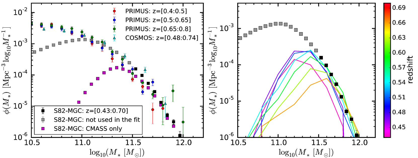
Bundy et al. (2015) present an estimate of the SMF at by using the s82-mgc catalog. In order to compute the SMF, Bundy et al. (2015) use a combination of spectroscopic redshifts, supplemented with photometric redshifts (photo-z’s) when a spectroscopic redshift is not available. We adopt a similar approach and compute the SMF from the s82-mgc at over . Our analysis assumes that the SMF does not vary over this redshift range. The result is shown in Figure 1. Error bars on the SMF represent the square root of the diagonal component of the covariance matrix, which is estimated from the data using 214 nearly-equal area bootstrap regions.
Because the majority of galaxies at the high mass end have a spectroscopic redshift, the impact of photo-z uncertainty on the Stripe 82 SMF is negligible (see L15), i.e., the use of photometric redshifts only adds a negligible amount of scatter in the total stellar mass estimate and does not inflate the high mass end of the SMF.
The left panel of Figure 1 presents a comparison between our SMF with results from COSMOS (Leauthaud et al., 2011) and PRIMUS (Moustakas et al., 2013) at similar redshifts. Figure 1 demonstrates that, because of the large area covered by Stripe 82, the high mass end of the total SMF is tightly constrained at over , while COSMOS and PRIMUS constrain the low mass end. The comparison with COSMOS and PRIMUS suggests that the s82-mgc is complete to at (Bundy et al., 2015).
We will use the s82-mgc SMF measured using 8 data points over the range . The inverse covariance matrix for the s82-mgc SMF, is computed as follows. First we compute the covariance matrix from 214 bootstrap regions, and then smooth the noise in the non-diagonal components using a boxcar algorithm (Mandelbaum et al., 2006). Finally we multiply by the Hartlap correction factor which is , i.e., . Although the error budget is dominated by the Poisson noise which only contributes to diagonal components (Smith, 2012), the Poisson error underestimate the errors. We find that the diagonal component in our jackknife covariance matrix is larger than the Poisson errors by a factor of in the mass range of our interest.
3.3 SMF of CMASS galaxies as a Function of Redshift
The other ingredient that will be important in our analysis are the SMFs of CMASS galaxies as a function of redshift. The right panel of Figure 1 shows SMFs for CMASS galaxies measured using the s82-mgc in 7 redshift bins with . As can be seen from the right panel of Figure 1, the completeness of CMASS depends both on redshift and stellar mass; this is because the effects of the magnitude and color cuts that define the CMASS sample vary with redshift. The utility of the these CMASS SMFs will be apparent when we describe our methodology in Section 5.
4 Subhalo Catalog
In this section we present the N-body simulation and subhalo catalog that is an essential ingredient in our abundance-matching study. We also perform tests of the completeness of the subhalo catalog.
4.1 N-body Simulation
Because the BOSS DR10 CMASS sample covers a large comoving volume, , with a high number density of , our analysis requires a large volume N-body simulation that can resolve halos to . We use the publicly available MultiDark simulation, MDR1 (Prada et al., 2012; Riebe et al., 2013). The cosmological parameters in MDR1 are consistent with a flat WMAP5 CDM cosmology (Komatsu et al., 2009): , , , , and . This cosmology is similar to the one used for our measurements of the clustering signals, therefore safely ignore the cosmological uncertainty in the distance scale (More, 2013). MDR1 is a simulation with a particle mass of ( particles). We use an output at which is close to the the peak of the BOSS CMASS at .
4.2 Halo Catalogs and Merger Trees
Halos and subhalos are identified using the Rockstar algorithm (Behroozi et al., 2013b; Behroozi et al., 2013a). Rockstar is a phase-space halo finder that also considers halo merger histories to provide a robust and stable identification of halos and subhalos. The advantages of Rockstar compared to other halo finders are well documented in Knebe et al. (2011) and Onions et al. (2012). These studies suggest that among halo finders, Rockstar finder is the least sensitive to resolution effects. Rockstar, with the Consistent Trees algorithm, produces halo merger trees and catalogs with various parameters derived from the halo assembly history, including, for example, , the maximum halo circular velocity for each subhalo.
We use the “”-axis of the MDR1 simulation as the line-of-sight direction. In order to maximize the volume of our mock, we re-map the 1-Gpc MDR1 cube into a cuboid of dimensions, following the method developed by Carlson & White (2010). After remapping, the -axis has a length of corresponding to a redshift range of . This includes a margin that is sufficient to account for peculiar velocities at the boundary of our mock catalog.
Peculiar velocities of subhalos are defined as the average velocity of particles within the innermost 10% of the virial radius. The virial overdensity in Rockstar is defined by at . This definition does not correspond to the definition of the halo bulk flow velocity that uses all particle members of the halo, because the halo core and its outer regions have different velocity structure. For a demonstration of this point, see Figure 11 of Behroozi et al. (2013b) and also Appendix B of R14.111The definition of halo peculiar velocity in R14 is the average of particles within of the virial radius where . All subhalos are mapped into redshift space by including the peculiar velocity component along the direction before performing abundance matching.
4.3 Time evolution and Resolution Tests
In this section, we discuss potential issues in the subhalo catalog, focusing in particular on the time evolution of subhalo clustering and completeness issues due to the resolution of the simulation. Here we only summarize our findings – Figures and further details can be found in Appendix. A.
We adopt a single redshift output at from the MDR1 simulation. We test if a single redshift output is sufficient to model CMASS over the redshift range . There are three outputs available in the MDR1 simulation over the redshift range of interest: and . Using these redshift outputs, we find a difference in the real-space correlation function at fixed number density, , at the % level at large scales. The largest differences (at the level of 5%) are seen at the 1-halo to 2-halo regime at (see Appendix. A). This level of evolution is below our measurement errors, but these effects will need to be taken into account in future work, especially when the of the measurements increases (currently we are using DR10 measurements).
We also perform two tests concerning the impact of the resolution of MDR1 on our results. First, we determine if the subhalo catalog resolves the mass scale required for our abundance matching. Based on White et al. (2011) and R14, we estimate that abundance matching for CMASS will require subhalos with . Our tests demonstrate that MDR1 resolves halos down to .
Second, we examine the impact of resolution effects on the radial profiles of subhalos. Our estimates suggest that subhalo radial profiles become incomplete at - (and depend on the ratio between the peak velocity of hosts and subhalos). The smallest scale in our measurement is and is close to this incompleteness limit. The impact of resolution on our results is at least partly counteracted by the boost to the errors of our measured by systematic fiber-collision correction uncertainties on these scales. We conclude that the resolution of MDR1 is sufficient for our purpose, but that recently-completed higher resolution simulations such as Skillman et al. (2014) or Ishiyama et al. (2014) would be preferable and will be adopted in subsequent work.
5 Methodology
Our goal is to find a model of the CMASS-halo connection which can simultaneously explain the SMF and the two-point correlation function and which also accounts for stellar mass completeness of CMASS. This section explains the details of our methodology. In this paper we only explore models that reproduce the projected two-point correlation function of the full CMASS sample over the redshift range of . In future work we will explore how well our models match the clustering of sub-samples (e.g., dividing CMASS by color and redshift).
We begin with a broad overview of our global methodology and the two classes of models explored in this paper. The details of our approach are then provided in the later half of this section. The casual reader may wish to read the overview of the methodology and then skip directly to the summary provided in Section 5.6.
5.1 Overview of Methodology and Models
Our approach is based on the SHAM framework for connecting galaxies and dark matter halos (see Section 5.2). Within the context of SHAM, we will explore two broad classes of models that relate galaxy color to halo properties. The first model that we explore is a “stochastic model” in which at fixed stellar mass, galaxy color in high-mass halos is simply a random process that does not correlate with halo properties. We will refer to this model as the “AbM" model. After abundance matching our mock catalog, we tag CMASS galaxies by randomly down-sampling the full mock galaxy catalog in such a way that the mock CMASS SMFs reproduce the ones measured in Section 3.3. Unless an additional correlation between this CMASS flag and halo properties is explicitly introduced, this procedure makes the implicit assumption that at fixed stellar mass, CMASS galaxies are a random sample of the overall population. However, L15 show that at fixed stellar mass, CMASS is not a random sample of the overall population in terms of galaxy color. Hence, the abundance matched catalog that we obtain after the down-sampling procedure will only correctly represent the true relation between galaxy color, stellar mass, and halo properties if color is a random process at fixed stellar mass.
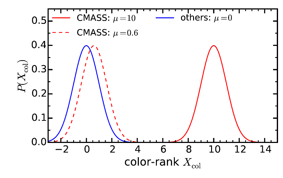
The second model is an extension to the traditional abundance matching scheme introduced by H13 called age matching. This model is based on the premise that galaxy color correlates with a secondary halo property at fixed stellar mass (see Section 5.3). After first abundance matching our mock catalog, the age-matched model will be built by re-shuffling CMASS galaxies according to a secondary halo property. In order to fully implement the age-matching model, however, we need to characterize the color distributions of galaxies from the s82-mgc as a function of mass and redshift and also to understand the effects of scatter introduced in these color distributions from photometric redshifts. This is a non-trivial task that we defer to Paper II - opting here instead to simply perform a qualitative investigation of the effects of age matching on the two-point correlation function. For this purpose, we will adopt a simple color model for the galaxy population that is based on a “color-rank distribution” represented by which effectively characterizes the color ranking of the CMASS versus other galaxies. This distribution is characterized by one free parameter called . As described in §5.3, this parameter controls the correlation strength between subhalo properties and the CMASS selection function.
5.2 Subhalo Abundance Matching
The SHAM scheme provides an effective and simple way to model the galaxy-halo relation and has been successful at modeling both the galaxy stellar mass function as well as the galaxy two-point correlation function (see e.g., Kravtsov et al., 2004; Vale & Ostriker, 2004; Conroy et al., 2006; Moster et al., 2010; Behroozi et al., 2010). The basic philosophy of SHAM is that massive (sub)halos host bright galaxies. More concretely, the SHAM method begins by rank ordering galaxies by stellar mass (or luminosity). Halos drawn from -body simulations are rank ordered by peak maximum circular velocity . Galaxies are then assigned to subhalos in descending order such that . In practice, there are multiple ambiguities in the SHAM technique. First, there is freedom in choosing how to rank order subhalos. For example, Reddick et al. (2013) showed how the predicted two point correlation function varies when rank ordering is performed using different halo mass proxies such as halo mass , maximum circular velocity , and its peak over entire merging history, . Motivated by this work, we will evaluate how our model varies when rank ordering by either or . Second, SHAM models must also account for scatter between galaxy properties and halo properties. We account for scatter by adopting the methodology of Behroozi et al. (2010) and Reddick et al. (2013).
To perform abundance matching, we need to evaluate the total SMF over the entire mass range covered by the CMASS sample, i.e., down to . This value is below the completeness limit of the s82-mgc. Our strategy will be to fit the total SMF from the s82-mgc in the range using a double Schechter function (Baldry et al., 2008):
| (6) |
where and the second term dominate at the low-mass end. The amplitude of the SMF below is unconstrained by the s82-mgc SMF but will be adjusted by our joint fit to the clustering of CMASS galaxies. Section 6 shows that our joint fit to the s82-mgc SMF and to yields a SMF that is consistent at the low-mass end with results from PRIMUS and COSMOS.
We abundance match subhalos against this SMF, and convolve it with a uniform log-normal scatter,
| (7) | |||||
which introduces a scatter in the relation between stellar and halo mass. This scatter arises due to a combination of intrinsic scatter in the stellar-to-halo-mass relation and errors associated with stellar mass measurements (Behroozi et al., 2010; Leauthaud et al., 2011). Hence, for a realistic model, the value of must be equal to, or greater than, the measurement errors in stellar mass measurements – we will return to this question in Section 6.
We fit the s82-mgc SMF over 8 data points at . Our SMF measurements probe the high mass end of the stellar mass function and hence are insensitive to some parameters in the double Schechter function. For this reason, in our fits, we simply fix the parameters that is not sensitive to the very high mass end to . This is motivated by results at the low-mass end from Baldry et al. (2008). In summary, our abundance matching model contains three free parameters, , , and .
We compute a for the s82-mgc SMF as follows:
| (8) |
where is the theoretical SMF predicted by Equation (7).
5.3 Subhalo Age Matching
SHAM essentially specifies the stellar-to-halo mass relation between galaxies and halos. It is normally assumed that halo mass is the primary variable on which the galaxy-halo connection depends. However, in addition to halo mass, halo clustering also depends on other parameters such as halo age, a phenomenon known as assembly bias (see e.g., Gao et al., 2005; Wechsler et al., 2006; Jing et al., 2007; Gao & White, 2007; Dalal et al., 2008; Li et al., 2008; Lin et al., 2015; Miyatake et al., 2015).
H13 introduced an extension to the traditional abundance matching scheme called age matching which can reproduce the color-dependent clustering of the SDSS main galaxy sample (also see Masaki et al., 2013). This method matches galaxies and halos using both stellar mass as well as galaxy color. The basic premise of the approach is that redder galaxies are assigned to older subhalos at fixed stellar mass.
In the age matching scheme, each halo is assigned a characteristic redshift () computed from halo merger trees. This parameter is defined as the maximum of three distinct age components:
-
•
: the earliest redshift at which the most massive progenitor of a given subhalo exceeds . For subhalos less massive than , .
-
•
: the epoch when a subhalo accretes onto a host halo. For host halos, .
-
•
: the epoch defined by , motivated by the fact that there is a tight correlation between the concentration parameter and the epoch when halo growth transits from a fast to slow accretion regime (Wechsler et al., 2006). Note that .
We adopt while in the original work of H13, .
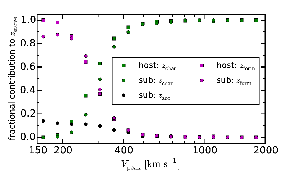
There is a critical difference between this work and H13: our relevant mass regime () is much higher than that of H13 (). H13 found that is the dominant component of for the SDSS main sample whereas we find that is the dominant component for CMASS (see Section 6). This is in keeping with the results shown in Figure 5 of Hearin et al. (2014b), which demonstrates that begins to dominate the contribution to for stellar masses at . In our CMASS sample, these higher-mass galaxies dominate the sample, whereas the Main Galaxy Sample is dominated by lower-mass galaxies. Because of these key differences, the impact of assembly bias in our models will be qualitatively different compared to H13 (see Section 6).
In Paper II we will use the actual color distributions of massive galaxies as a function of redshift to perform age matching. Our goal in this paper, however, is to perform a first qualitative analysis of the general effects of age matching above collapse mass, a regime that has not yet been fully investigated. For this purpose, we introduce a simple color-rank distribution denoted . This color-rank distribution will be used to assign “colors” to CMASS and to non-CMASS galaxies and to perform the color-based rank ordering in the age matching scheme. Our goal is to construct a model that allows for a simple “mixing” between these two populations.
Operationally, we accomplish this mixing with our age matching model as follows. First, at each stellar mass we generate a random distribution of values. Suppose there are subhalos in the stellar mass bin, and that the fraction of galaxies of this stellar mass that are CMASS-selected is denoted by We then draw values from a Gaussian distribution of mean and unit variance; these draws will be the “colors" of our mock CMASS galaxies. We next draw values from a Gaussian distribution of zero mean and unit variance; these draws will be the “colors" of our non-CMASS galaxies. We then rank-order the joint collection of the randomly drawn values of Subhalos in the same stellar mass bin are rank-ordered by . In monotonic fashion, the larger draws are assigned to the subhalos with larger values, and the CMASS-designation associated with is also assigned to the subhalo, defining the CMASS selection function in the “AgM" model.
The value of determines the strength of the correlation between the CMASS selection function and subhalo at fixed stellar mass. If is large (for instance, ), then values with a CMASS-designation are always larger than values attached to non-CMASS draws, in which case at fixed stellar mass, subhalos with the highest are always selected to be CMASS galaxies. On the other hand, if , the distributions of CMASS and non-CMASS draws are identical, so in this case matching the and distributions has no impact on the CMASS designation assigned to the subhalos, and the CMASS selection function is uncorrelated with at fixed stellar mass. Finally, for intermediate values of (for instance, ), then CMASS and non-CMASS galaxies have overlapping distributions, but CMASS galaxies are “redder" on average. Figure 2 illustrates these concepts.
In our analysis, is left as a free parameter which means that we determine the degree to which CMASS colors overlap with non CMASS galaxies directly from the data. We do not however currently account for any redshift and stellar-mass dependence of , thus we do not account for any redshift and stellar-mass dependence of the CMASS color-cuts. This is a limitation of our current model, the importance of which will become clearer in Section 6.3.
5.4 Accounting for the Stellar Mass Completeness of CMASS as a Function of Redshift
We assume a single global SMF over the CMASS redshift range. For each set of parameters , we create a mock catalog via abundance matching. At this point galaxies in the mock catalog have redshifts and stellar masses. The next step is to tag CMASS galaxies in the abundance-matched mock catalog as a function of redshift. We divide our simulation into seven redshift bins along the direction (the bin width is ). The redshift width of is conservative and this choice is motivated by the uncertainty of photometric redshift estimation in the s82-mgc catalog.
The CMASS SMF varies as a function of redshift as a result of the BOSS selection function. In Section 3.3, we used the s82-mgc catalog to measure the number densities of CMASS galaxies as a function of mass and redshift, . Because we assume that the total SMF does not vary over our redshift baseline, we can compute how many CMASS galaxies are expected for every redshift slice in the mock catalog simply by scaling this number by the ratio of volume in the redshift slice in the mock () to the s82-mgc volume ():
| (9) |
In order to predict the number of mock galaxies as a function of mass and redshift, we construct bins in stellar mass from 10.6 to 12.3 dex with . We have checked that our prediction is stable with . In the mock catalog, we randomly tag galaxies with a CMASS flag. For a small number of bins, exceeds the number predicted by the total SMF (simply due to sample variance). In this case, we simply set . Following this procedure, every galaxy in our mock catalog is now assigned a stellar mass, a redshift, and a flag that indicates mock CMASS galaxies. By design, mock CMASS galaxies have stellar mass distributions that match the ones measured in Section 3.3.
5.5 Predicting the CMASS Two-Point Correlation Function
We now have a mock catalog that contains galaxies with three dimensional positions and with a flag that indicates CMASS galaxies. The next step is to compute the predicted the CMASS two-point correlation function. is computed from the mock following the exact same procedure as for the BOSS DR10 data. To account for the finite volume of the simulation, we compute a covariance matrix for (referred to as ), which is estimated via jack-knife by dividing the -plane into 256 equal regions. For the small scales of concern in this paper, jack-knife errors outperform bootstrap errors (P. Norberg, private communication, Arnalte-Mur & Norberg et al., in prep).
The fitting for is performed with
| (10) |
where , and the total covariance matrix includes uncertainties in both measurement and our theory estimates, i.e., .
5.6 Summary of Methodology
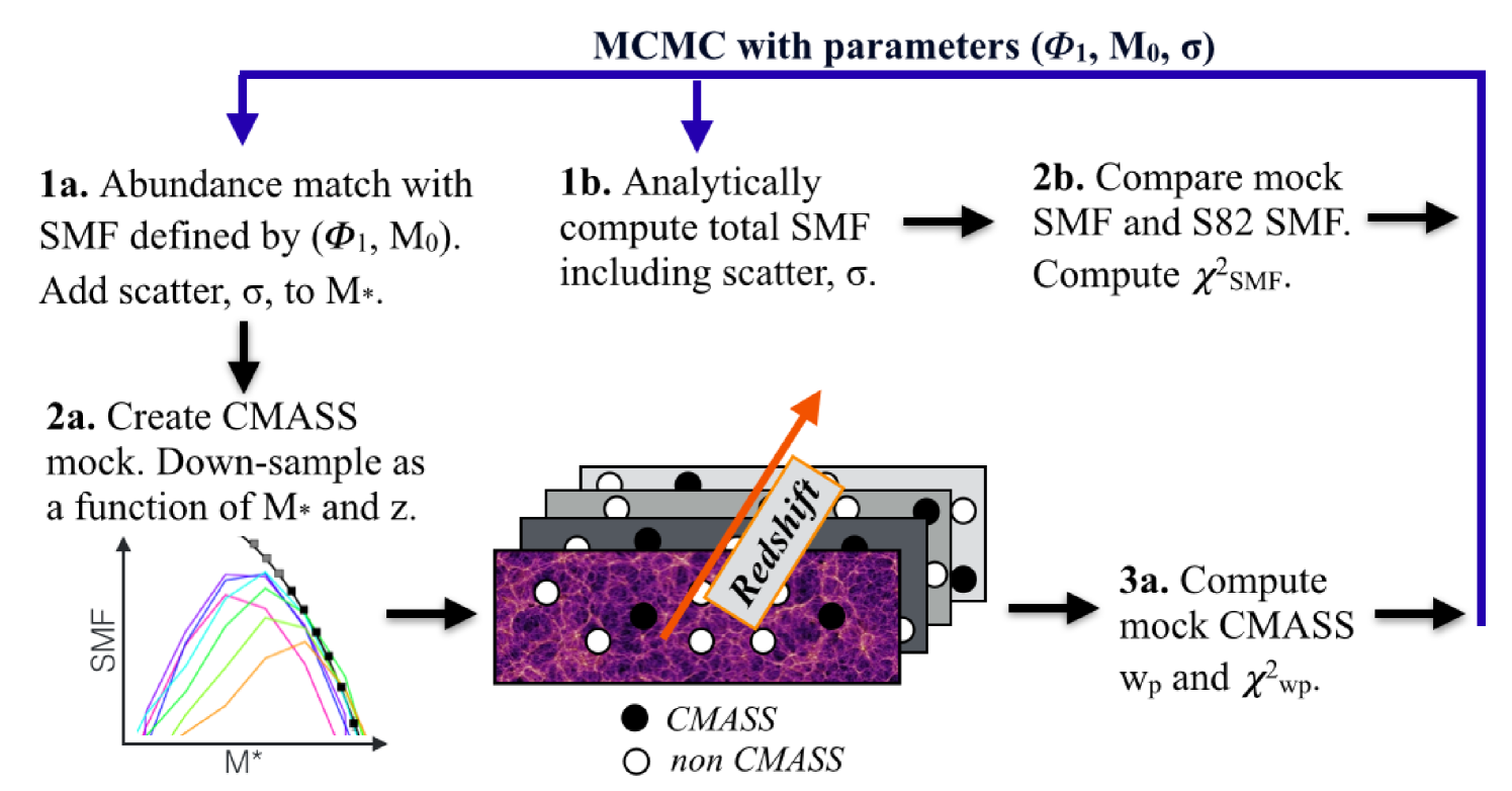
Figure 3 presents an illustration of our methodology for the AbM model. A summary of our methodology is as follows:
-
1.
Start with a set of SMF parameter values. For the stochastic (“AbM”) model, the parameters are . For the age-matching (“AgM”) model there is an additional parameter, . The parameter only impacts the modeling of two-point statistics such as - one-point statistics such as the SMF are entirely unaffected by
- 2.
-
3.
In parallel, we generate a mock catalog to model . The first step in generating this mock catalog is to abundance match the mock catalog using the same total SMF (without scatter) as in the previous step. We test abundance matching both in terms of and . Scatter () is introduced into stellar mass in the mock catalog at fixed (or ). We have checked that the mock catalog is large enough that stochasticity due to the rare number of high mass halos is a negligible effect, i.e., the Poisson error in the measured mass function dominates the error budget at high stellar masses.
-
4.
The direction of the mock is taken as the redshift axis. Mock CMASS galaxies are tagged in the mock catalog by down-sampling the overall population in redshift and stellar mass in order to reproduce the CMASS SMFs measured in Section 3.3.
-
5.
At this stage, mock CMASS galaxies are simply a random sub-sample of the overall population; this mock corresponds to our stochastic “AbM" model.
-
6.
For the age-matching model, we begin by assigning the subhalos a color-rank, , as follows. For subhalos hosting a non-CMASS galaxy, is drawn from a Gaussian distribution with zero mean and unit variance. For subhalos hosting a CMASS galaxy, is drawn from a Gaussian distribution with mean and unit variance. At fixed stellar mass, the random values are rank-ordered. At the same stellar mass, the mock galaxies are rank-ordered by a secondary halo property, where we choose as this secondary parameter in our fiducial model, where is concretely defined in §5.3. In monotonic fashion, the subhalos with the largest values are assigned the largest values, and the CMASS/non-CMASS designation associated with each value is also assigned to the subhalo.222For certain tests, we may rank-order the subhalos only according to or (Section 5.3). Thus subhalos in the “AbM" and “AgM" mocks in general have different CMASS-designations: in “AgM", the CMASS-designation is correlated with at fixed , with the correlation strength governed by our parameter.
-
7.
Generate a random catalog that follows the CMASS and compute . Note that is fixed using our best-fitting parameters (after a first initial iteration).
-
8.
Compute between and , and then add as .
-
9.
Iterate this procedure.
The best-fit parameters and errors are determined using the Markov chain Monte Carlo (MCMC) technique. We use a modified version of COSMOMC (Lewis & Bridle, 2002) that has been well tested in previous work (Saito et al., 2011; Zhao et al., 2013; Saito et al., 2014). Since our SMF is estimated from s82-mgc and the correlation function is computed over the full DR10 footprint, the cross correlation between these two statistics are negligible. The for the multipoles is defined in a similar way. The correlation between the monopole and the quadrupole is properly taken into account by the covariance matrix.
6 Results
6.1 Abundance Matching
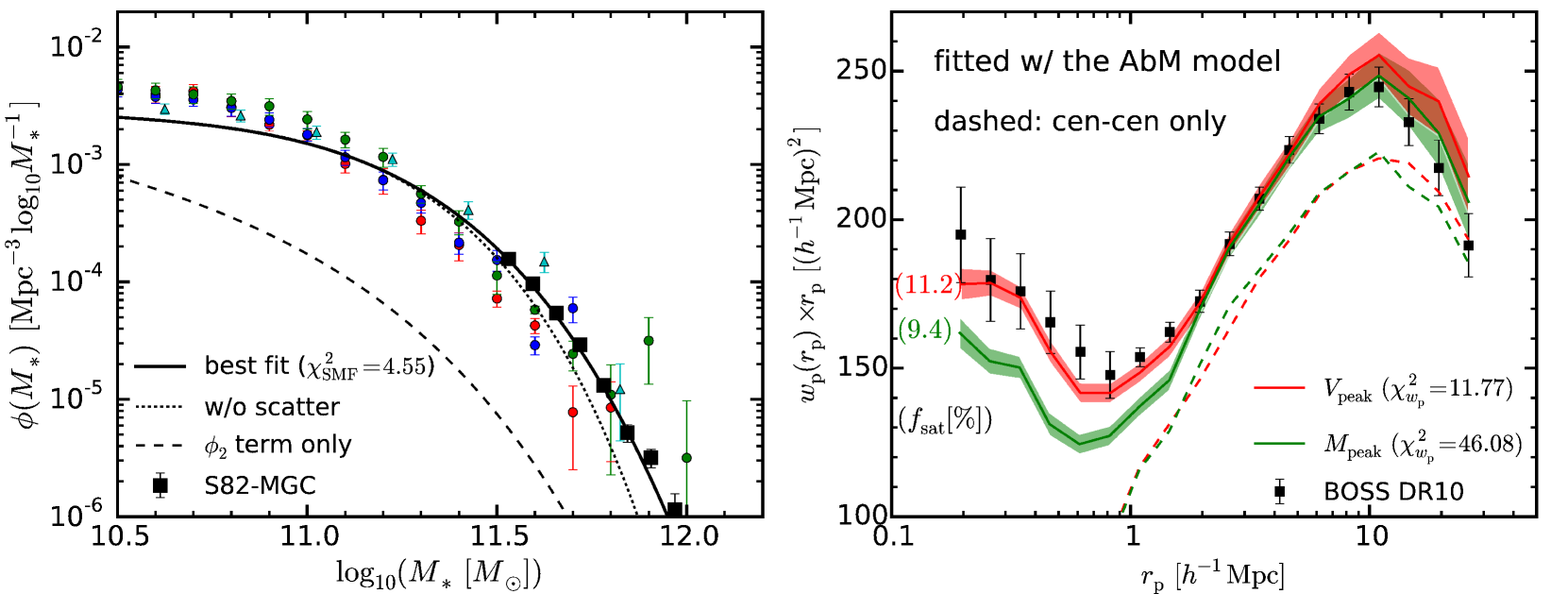
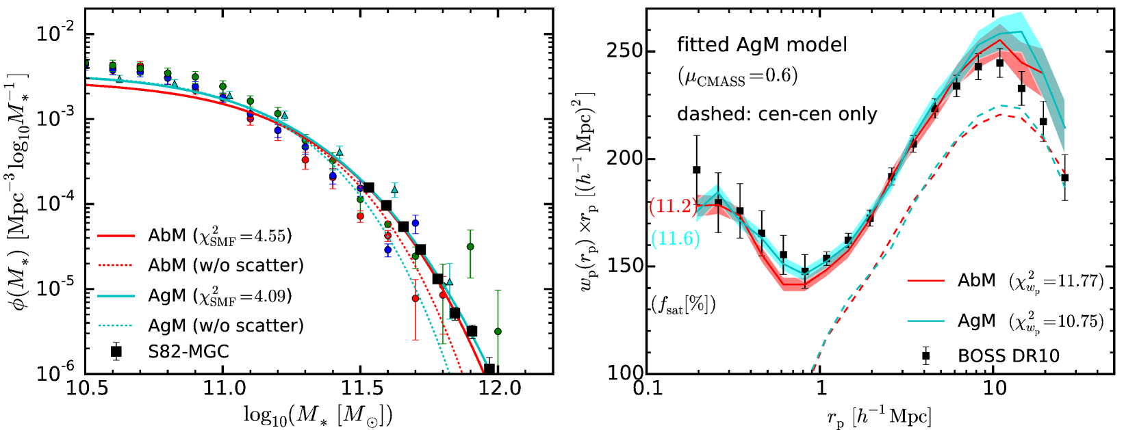
We now perform a joint fit to the SMF and to . The left panel of Figure 4 presents our best-fit to the SMF using a double Schechter function and abundance-matching against . The best-fit parameters for the double Schechter function are: with . Errors are reported with a 68% confidence level. We find excellent fits to both the SMF and with two specific points worth highlighting. First, the amplitude of our best fit SMF agrees well with COSMOS and PRIMUS at but has a lower amplitude at . Because the number density of CMASS drops sharply below this mass scale, we simply do not expect to constrain the total SMF in this range. Second, the best fit value for the scatter is lower than our naive expectation. Indeed, should include contributions from measurements errors as well as from intrinsic scatter in the stellar-to-halo mass relation. The average uncertainty in stellar mass measurements from the s82-mgc is of order dex in this mass and redshift range. Hence, a value of implies a very small intrinsic scatter in the stellar-to-halo mass relation. We will return to this point in the discussion section.
The right hand panel of Figure 4 presents our best-fit to as the red line (). The goodness of fit in this case is . We have also tested abundance matching against instead of . The blue line shows the results of abundance matching against using the same best-fitting SMF parameters as above. As can be seen from Figure 4, yields a larger clustering amplitude and is more consistent with the BOSS data than .
There are two factors which lead to the differences in these clustering predictions. First, host halos selected by cluster more weakly relative to host halos selected by as discussed in Zentner et al. (2014). This effect is small in our halo mass range, which we have verified by comparing the central-central pair counts between the two models, which are nearly identical. Second, the satellite fractions predicted by the two models are different: our based SHAM model has a larger satellite fraction relative to the based model. Indeed, at fixed , subhalos have larger than host halos (see Figure 2 in Reddick et al., 2013), which suggests that rank-ordering with results in similar clustering of central galaxies but the larger satellite fraction boosts the overall clustering amplitude. We adopt as our fiducial model and do not explore abundance matching with any further.
6.2 CMASS
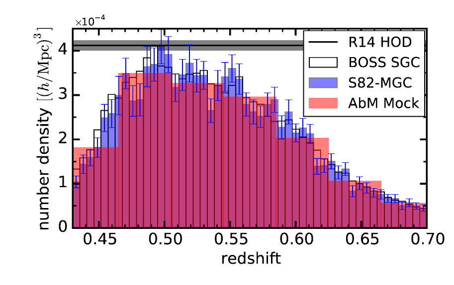
Figure 5 presents a comparison between the redshift distribution of CMASS galaxies from our best-fitting mock catalog with the redshift distribution of CMASS galaxies in the s82-mgc and from the full BOSS DR10 SGC. Our mock reproduces the CMASS from the s82-mgc catalog and is consistent with from the BOSS DR10 SGC. The amplitude differences between the from our mock and the DR10 are due to sample variance. In our current methodology, the sample variance introduced by matching the CMASS SMFs from Stripe 82 is not taken into account which is a limitation of our current approach. This reflects a trade-off made to take advantage of the higher quality stellar mass estimates from the s82-mgc, but doing so, our current analysis is also limited by the sample variance from Stripe 82.
6.3 Gaining an Intuition for Age Matching Above Collapse Mass
In the previous section, we showed that a reasonable fit to and can be achieved using a simple abundance matching scheme in which galaxy color in high mass halos is simply a stochastic process. We now investigate whether or not models in which galaxy color correlates with halo assembly properties can achieve comparable results. One caution worth mentioning here with respect to the age matching model is that, unlike in H13, the combination of the steep relation and the non-zero scatter in this relation leads to a difference in the mean host halo mass compared to the standard abundance matching model (see Appendix. B for details).
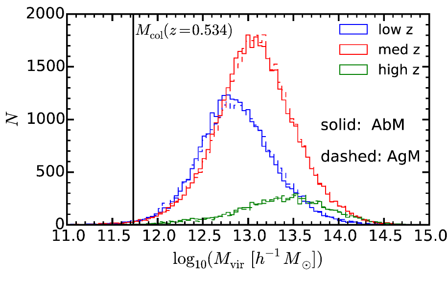
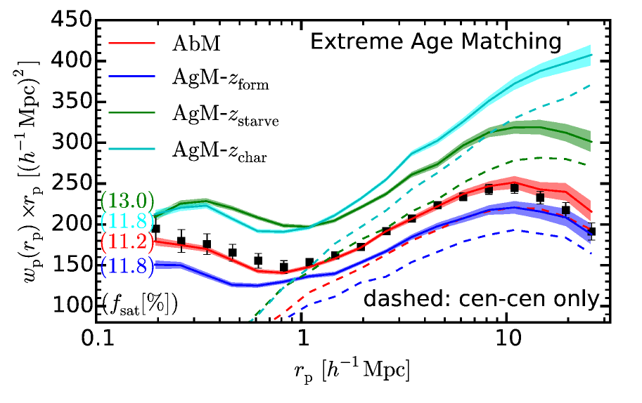
First, we wish to develop some intuition for how the different components of affect in this high halo mass regime. Figure 6 shows that CMASS galaxies are firmly in halo masses above collapse mass, . Hence, the behavior of may be fundamentally different compared to previous work by H13. Let us begin by considering an extreme case in which CMASS galaxies are all redder than non-CMASS galaxies (, see solid lines in Figure 2). For this test, we adopt the values of the best fit to from Figure 4 . At fixed stellar mass, we rank order galaxies according to , , or . The results of this extreme case are presented in Figure 7. Interestingly, but perhaps not surprisingly, we find that (blue curve) lowers the clustering amplitude. This is because is defined using halo concentrations and the effects of assembly bias have an opposite effect above and below collapse mass when using the concentration parameter (see e.g. Wechsler et al., 2006; Dalal et al., 2008). Thus, in this high-mass regime, causes red galaxies to cluster less strongly than blue ones.
Let us now turn our attention to . Interestingly, rank ordering according to produces the opposite effect and causes an increase in the clustering amplitude. Previous work on assembly bias has shown the switch in the assembly bias effect seen when considering halo concentration is not always reflected when considering other halo parameters. Previous work has not studied the specific case of ; however, Jing et al. (2007) and Li et al. (2008) report that when an age parameter based on a fixed mass threshold such as is used where denotes the redshift when a halo acquires half of the final mass at the observational time, a similar behavior is observed (see Figure 4 in Li et al., 2008).
Finally, let us now examine the component, which includes contributions from both and . The prediction for lies between the and the cases but is closer to than to . This is because in this mass regime, is dominated by not (see Figure 8). Thus the impact of the assembly bias for CMASS is qualitatively distinct from the trends identified by H13 in lower mass halos, a fact which traces to the change in character of assembly bias for halos above and below collapse mass.
The dashed curves in Figure 7 display for central galaxies only – demonstrating that the trends discussed above are not simply due to varying satellite fractions.
6.4 Fit to with an Age Matching Type Model
Of course, the true differences between the color distributions of CMASS galaxies compared to non-CMASS galaxies of similar mass are not as extreme as the case explored in the previous section. As discussed in section 5.1, the implementation of age-matching first requires a characterization of the color distributions of galaxies from the s82-mgc as a function of mass and redshift and also requires modeling the effects of scatter introduced in these color distributions from photometric redshifts. This is an aspect that we defer to Paper II. Here, we perform a qualitative investigation of the effects of age matching on the two-point correlation function using the color-rank variable .
We now perform a joint fit to the SMF and to in which is left as a free parameter (the “AgM” model). The results are presented in Figure 9. The best-fit parameters are with and . The AbM model and the AgM model yield a comparable goodness of fit ( for the AbM model and for the AgM model). There are three points worth highlighting concerning the results of the AgM model. First, the best-fit SMF has a slightly higher amplitude at low stellar masses compared to the AbM model and is in better agreement with PRIMUS and COSMOS. Second, the best-fit value for the scatter is larger than the AbM model ( versus ), which leaves a larger margin for intrinsic scatter. Finally, the best-fit value for of corresponds to a scenario in which CMASS and non-CMASS galaxies have overlapping color distributions, but with CMASS galaxies being somewhat redder on average. Reassuringly, this result matches our qualitative expectations for this sample.
The AgM model explored here is simplistic in the sense that we have used a single value of over a whole CMASS redshift range, whereas the true color distribution of CMASS versus other galaxies depends on redshift. A more sophisticated model which accounts for this effect will be presented in a forthcoming paper.
7 Discussion
7.1 HOD Modeling in the Context of Complex Samples such as CMASS
Both HOD and SHAM are popular methods for modeling the SMF and the galaxy-two-point correlation functions. One reason that HOD methods are popular is that they provide a relatively simple framework that can also be used to rapidly model a variety of observables. However, one of the downsides of this method is that specific functional forms must be assumed for the central and satellite occupation functions. These assumptions may be robust for volume-limited threshold samples such as those commonly studied in the SDSS main samples (e.g., Zehavi et al., 2011). However, it is less clear if these types of methods can be applied to samples such as CMASS which are selected via complex color and luminosity cuts and for which both the shape and normalization of the effective HOD may vary with redshift.
There have been several attempts to model the CMASS-halo connection on the basis of HOD type models. Among these studies, Guo et al. (2013, 2014) and More et al. (2014) focused on specific sub-samples of CMASS, whereas White et al. (2011) and R14 used a HOD type model to describe the clustering of the full CMASS, assuming no redshift evolution in the HOD.
In this paper, we have introduced a novel SHAM-based method333After this paper was submitted, a parallel effort was brought to our attention which adopts a similar methodology as our paper (Rodríguez-Torres et al., 2015). that can be used to model complex populations such as CMASS by accounting for the mass completeness of the sample as a function of redshift. We explore a first qualitative approach for also considering color completeness which will be developed further in Paper II. We now investigate what these models predict in terms of the redshift dependence of the CMASS HOD. The right panel of Figure 1 shows that the SMF of CMASS varies strongly with redshift. This figure alone suggests that the HOD of the CMASS sample is not likely to be uniform over the CMASS redshift range.
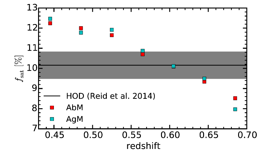
Figure 10 presents the HODs predicted from our AbM and AgM mock catalogs as a function of redshift. As a comparison we also display the HOD from R14, which assumes no redshift evolution. R14 fit the clustering assuming a constant number density with a derived value of (see Figure 5) under the assumption that the CMASS can be obtained by simply down-sampling the best-fit HOD as a function of redshift. We down-sample the R14 HOD to match the CMASS and present the results in Figure 10.
There are several noteworthy differences between our HODs and the single non-evolving one from R14. At the lowest redshift bin, , the mean occupation for central galaxies does not approach unity due to incompleteness in the SMF at high mass end (see the magenta curve in the right panel of Figure 1). At , which corresponds to the peak of the CMASS , our HOD is more similar to R14, but there is still a discrepancy in the shape of , especially at the low mass end. The largest differences are at . Our HODs converge to unity at large halo masses whereas the down-sampled R14 one converges to ; this is due to the stellar mass completeness of CMASS. This difference arises, because, in our models, the decline of the CMASS number density above is caused by the fact that the mean stellar mass of the sample increases (as constrained by data from the s82-mgc). In contrast, the fixed HOD of R14 must significantly down-sample the overall amplitude of the HOD to achieve comparable number densities.
Finally, our model predicts an evolution of the mean halo mass of CMASS, as a function of redshift. More specifically, our models predict that, at and , the mean halo mass of central CMASS galaxies is 13.12 (13.15), 13.34 (13.35), and 13.66 (13.68) for the abundance-matched (age-matched) cases, respectively. This variation is driven by the fact that mean stellar mass of the sample varies with redshift, as is clearly seen in the right panel of Figure 1. These values are compared with the HOD result, , which is higher (lower) than our results at low (high) redshift. In addition, our models predict that the CMASS satellite fraction varies with redshift from 12% to 9%, as shown in Figure 11. While this effect might seem like a small and negligible variation, the fiducial HOD from R14 constrains the satellite fraction at 6.8 % precision. It is interesting that the value inferred from the single HOD fit in R14 is consistent with our values at but that not at lower redshifts.
In conclusion, our work suggests that CMASS is a complex sample for which the HODs are likely to vary with redshift in a non-trivial manner. A single HOD fit to the overall broadly agrees with the predictions from our model at the median redshift of the sample. However, at lower and higher redshifts, our model predicts that HODs are not simple down-sampled versions of the HOD at the peak of the .
7.2 A Cautionary Tale of Modeling Small Scale Statistics
Many previous studies have used a combination of galaxy abundances and the projected galaxy two-point correlation function in order to constrain the galaxy-halo connection (e.g., Leauthaud et al., 2011; Coupon et al., 2015; Zu & Mandelbaum, 2015). However, just because SHAM or HOD models can reproduce these observables does not necessarily imply that the models accurately capture the true underlying galaxy halo connection, i.e., just because the model provides a good fit to the data does not necessarily imply that the model is correct. A clear illustration of this statement in the context of mock galaxy samples with strong assembly bias is discussed in Zentner et al. (2014). In this paper, we have studied two distinct models: standard abundance matching and a simplified form of age matching, abbreviated by AbM and AgM, respectively. We have demonstrated that both models can reproduce the galaxy SMF as well as , suggesting that there are fundamental degeneracies among traditional HOD model, AbM, and AgM models, in modeling the SMF and . This naturally leads to two interesting and inter-related questions.
-
1.
How well do these models predict other statistics derived from the data?
-
2.
Are there other statistics which can distinguish between these two distinct models?
Instead of considering just the projected correlation function, we turn our attention to the multipoles of the full 2D correlation function. Figure 12 shows the pseudo multipoles (see Section 3) for our best-fitting AbM and AgM models. The left panel of Figure 12 demonstrates that both models fail dramatically to reproduce the pseudo multipoles even though both models provide a satisfactory description of . In the following section, we will use the redshift dependent clustering of CMASS to argue that in addition to stellar mass, galaxy color must play an important role in determining the clustering of CMASS galaxies and that the failure of our model in reproducing the pseudo-multipoles must be a consequence of these effects.
In conclusion, our paper provides a clear cautionary example of the limitation of inferring the galaxy-halo connection from the projected correlation function alone. It is also clear from Figure 12 that the pseudo-multipoles contain additional information not captured by and that these may represent a powerful and under-utilized tool to provide additional constraints on the galaxy-halo connection. These aspects will be explored in greater detail in a forthcoming paper.
7.3 Redshift Evolution of CMASS Clustering
As discussed in section 7.1, one major difference between the R14 model and this work is the treatment of the redshift evolution of the CMASS sample. In R14, CMASS is assumed to be a single homogenous sample with a that is modeled by down-sampling a redshift independent HOD. In contrast, in this paper, the varying number density of CMASS is a direct result of the measured mass incompleteness of the sample as constrained by the 82-mgc catalog. We now explore the consequences of these differences by examining the redshift dependent clustering of CMASS.
The original motivation for the non-evolving HOD in R14 originates from the observation that the clustering of CMASS galaxies does not vary strongly with redshift. This is shown by Figure A1 in R14 (reproduced here in the right two panels of Figure 12). Because randomly downsampling galaxies does not modify their clustering, the R14 model leads to a constant clustering amplitude with redshift, which indeed, seems well supported by Figure 12. However, another consequence of this procedure is that the halo mass of the CMASS sample is constant with redshift in the R14 model. In contrast, the S82-MCG catalog shows that the stellar mass of the CMASS sample increases by a factor of 1.8 over the range which leads to a factor of 3.5 increase in the predicted mean halo mass of CMASS based on our SHAM modeling.
How much redshift evolution should we expect in the clustering of CMASS galaxies given this factor of 1.8 increase in stellar mass? The right hand side of Figure 12 presents the predicted redshift evolution of the pseudo-multipoles from our SHAM modeling. We find that the observed stellar mass variation of the CMASS sample should lead to more than a factor of 1.5 increase in the clustering amplitude over the CMASS redshift range444 Notice that we here ignore the redshift evolution in the MDR1 simulation. However, as seen in Figure. 13, the effect of the redshift evolution is at the level of 5%. . Figure 12 clearly reveals a fundamental contrast between the measured non evolution of the clustering of CMASS and the expectation based on the redshift-dependent stellar mass distributions. This discrepancy is qualitatively insensitive to the exact details of our SHAM methodology. The observed increase in stellar mass will lead to a roughy similar increase in halo mass (and hence clustering amplitude) independently of the exact halo parameter ( or ) used in the abundance matching.
We argue that the discrepancy revealed in Figure 12 suggests, in addition to stellar mass, galaxy color must also play an important role in determining the clustering amplitude of CMASS galaxies. Figure 5 in L15 demonstrates that CMASS galaxies display a range in star-formation histories at fixed stellar mass. At low redshift and fixed stellar mass, the CMASS selection function excludes galaxies that have experienced recent star formation. At higher redshifts (), the CMASS sample is mainly flux limited and includes a larger range of galaxy colors at fixed magnitude. A variety of lensing and clustering studies suggest that, for low mass galaxies, the clustering of blue galaxies is lower than red galaxies at fixed stellar mass (e.g., Tinker et al., 2013). It is not trivial that these trends persist in this very high galaxy mass regime, but if so, the inclusion of bluer galaxies in CMASS at higher redshifts may exactly compensate for the increase in the mean stellar mass. In other words, the observed constant clustering of CMASS may be due to a coincidental compensation between color and stellar mass with redshift.
7.4 What Determines Color in the Most Massive Galaxies?
One of the main goals of this paper is to understand the connection between halo properties and the colors of very massive galaxies. As shown in Figure 6, CMASS galaxies live in halos with halo masses above . In this regime, gas accretion is thought to be dominated by the “hot halo mode” and heated by pressure-supported shocks to a temperature that limits star-formation (Dekel & Birnboim, 2006). In addition, at these halo masses, “maintenance mode” feed-back mechanisms, such as radio-mode feed-back, are thought to further limit star-formation in the most massive galaxies Croton et al. (2006). However, massive galaxies at these redshifts are observationally not all red and dead. The CMASS sample in fact contains a blue population (Guo et al., 2013; Ross et al., 2013). Based on high-resolution Hubble Space Telescope imaging, Masters et al. (2011) estimate that of the CMASS sample has a late-type morphology associated with the star-forming disk (Masters et al., 2011). Using a maximum likelihood approach that accounts for photometric errors as well as the CMASS selection cuts, Montero-Dorta et al. (2014) estimate that 37% of CMASS object may intrinsically belong to the blue cloud.
Semi-analytic models (SAMs) sometimes assume that galaxy color in high mass halos is a stochastic process. For example, Lu et al. (2014) adopts a simplified halo quenching model to mimic the effects of AGN feedback that stops radiative cooling in high-mass halos. In this model, radiative cooling is randomly switched off when halos reach a critical mass of (with a Gaussian spread of 0.3 dex). In Benson (2012), the galacticus model is more sophisticated and follows the growth and spins of black holes. The AGN jet power is computed from the accretion rates and spins of the black hole and is used to counterbalance radiative cooling in the hot halo. The parameters of the galacticus model are tuned to produce a transition around few in halo mass, such that quenching begins above that mass. In this sense, quenching will be stochastic at but also depends on the black hole accretion rate and spin. In the galacticus model, feedback may also shut down temporarily, for example after a merging event with high accretion rates which causes the black hole accretion disk to transition to a thin (radiative) mode with weaker jet power.
It is thus interesting to ask what drives color in massive galaxies which live in halos above . Is color a stochastic processes that is simply linked to small episodic amounts of gas cooling and/or merging events? Or is the color in massive galaxies linked to halo properties such as halo age and hence perhaps more fundamentally tied to the large scale reservoir of fuel and the assembly history?
Our current paper does not fully account for the color selection of CMASS but we can address some of the questions above. In our AbM model, galaxy color is randomly assigned at fixed stellar mass. In the AgM model, on the other hand, color is correlated with and hence with subhalo age. The degree to which color correlates with is left as a free parameter and determined from the data. We have shown that both models can reproduce the galaxy SMF as well as but fail to match the pseudo-multipoles.
To begin, let us focus on the consequences of Figure 12 in terms of the AbM model. Because the mean stellar mass of the CMASS sample increases with redshift, the AbM model predicts a strong variation in the clustering amplitude with redshift which is clearly ruled out by the data. Hence, we argue that the stochastic color model (i.e., the AbM model) can be ruled out with high significance by our analysis.
We now turn our attention to the AgM model. Our current implementation of the AgM model provides an excellent description of the SMF and but fails to reproduce the pseudo-multipoles. However, unlike in the case of the AbM model in which the redshift dependence of the color cuts are unimportant, we know that our AgM model will be sensitive to these effects which we have treated in a simplistic fashion. In a forthcoming paper, we will investigate if a more realistic AgM model which accounts for the color completeness of CMASS with redshift can describe the redshift dependent multipoles. This approach should provide with powerful constraints on the physical mechanism that drives galaxy color in massive halos.


8 Summary and Conclusions
The last decade has seen rapid observational progress in our understanding of the relationship between galaxies and their underlying dark matter halos, However, the connection between galaxies and dark matter remains poorly constrained for massive galaxies with because these galaxies are rare with low number densities, and require large areas surveys to obtain statistically significant samples. The BOSS survey provides a spectroscopic data set of massive galaxies at intermediate redshifts with number densities of in a survey volume that covers several cubic Gigaparsec (the “CMASS” sample). This gigantic dataset enables high-signal-to-noise ratio measurements of three dimensional galaxy clustering of massive galaxies.
In this paper, we introduce a novel method based on the SHAM framework that can be used to model complex populations such as CMASS by accounting for stellar mass (and eventually color) completeness as a function of redshift. CMASS is referred to as a “constant stellar mass” sample but L15 demonstrate that CMASS is only truly stellar mass limited in a narrow mass and redshift range. In order to fully utilize this sample to understand the galaxy-halo connection, it is critical to account for the CMASS mass completeness function. Our paper accounts for these effects and hence addresses an important limitation of the CMASS sample which has typically been neglected in previous work. Our mock catalogs account for CMASS selection effects, reproduce the overall SMF, the two-point correlation function of CMASS, and the CMASS ; the HOD table as a function of redshift; all made publicly available at www.massivegalaxies.com. After submitting our paper, a related effort by Rodríguez-Torres et al. (2015) was brought to our attention. Several key differences between Rodríguez-Torres et al. (2015) and our work include the choice of the input stellar mass function, as well as the methodology for introducing scatter between stellar and halo mass.
We use data from Stripe 82 to measure the total SMF down to and perform a joint fit to both the SMF and the projected two point correlation function of CMASS galaxies. Our SHAM model (our “AbM model") provides an excellent description of these two observables. Previous work has assumed that the CMASS HOD does not evolve with redshift. We re-investigate this assumption and show that the CMASS HOD should in fact vary strongly with redshift. Our model predicts that both the mean halo mass and the CMASS satellite fraction should vary with redshift. This variation is driven by the fact that the mean stellar mass of the sample increases at higher redshifts. In conclusion, our work suggests that CMASS is a complex sample for which the HODs are likely to vary with redshift in a non-trivial manner.
The color selection applied to the CMASS sample may cause the two-point correlation function to be sensitive to assembly bias effects. We study the impact of such effects on the two-point correlation function using the age matching framework recently introduced by H13. In contrast with H13, our sample lies firmly above collapse mass at , which corresponds to a relatively unexplored mass range. We demonstrate that in this regime, the effects of assembly bias are markedly different compared to the ones explored by H13 at lower stellar masses. For example, unlike H13, in this regime is dominated by and not by . Also, the component of causes red galaxies to cluster less strongly than blue ones. However, we also find that the rank ordering according to produces the opposite effect and causes an increase in the clustering amplitude. We show that an excellent fit to the CMASS two-point correlation function (which includes assembly bias effects) can be achieved by balancing these two opposing effects.
Overall, our two distinct models (standard abundance matching and age matching) can reproduce the galaxy SMF as well as , suggesting at first view a fundamental degeneracy between these models. However, we show that both models fail to reproduce the pseudo multipoles even though both models provide a satisfactory description of . Hence, our paper provides a clear cautionary example of the limitation of inferring the galaxy-halo connection from the projected correlation function alone.
We investigate the redshift dependent clustering of CMASS and find that the observed stellar mass variation of the CMASS sample should lead to more than a factor of 2.0 increase in the clustering amplitude over the CMASS redshift range which is in stark contrast with the data. We argue that this discrepancy suggests that, in addition to stellar mass, galaxy color must also play an important role in determining the clustering amplitude of CMASS galaxies and that the observed constant clustering of CMASS may be due to a coincidental compensation between color and stellar mass with redshift. Given a discrepancy in shape of the multipole correlation function, it may be necessary to consider velocity bias as recently studied in Reid et al. (2014); Guo et al. (2014) in the HOD framework. However, the velocity bias between subhalos and galaxies are not well investigated yet for the mass scale and redshift range of our interest, and we defer this aspect to future work (but see Guo et al. (2016) for such an effort against the SDSS main sample).
Finally, we discuss the physical processes that drive galaxy color in high mass halos. We are interested in determining if color in these massive galaxies is a stochastic processes that is simply linked to small episodic amounts of gas cooling and/or merging events. Or is color in massive galaxies linked to halo properties such as halo age and hence perhaps more fundamentally tied to the large scale reservoir of fuel and the assembly history? The stochastic scenario corresponds to our AbM model in which galaxy color is randomly assigned at fixed stellar mass. Because the comparison of the redshift dependent clustering of CMASS with our AbM model, we argue that the stochastic color model can be ruled out with high significance by our analysis. In this case, color in high mass halos may be linked to other properties besides halo peak velocity, suggesting that assembly bias effects may play a role in determining the clustering properties of this sample.
Our current implementation of age-matching also fails to reproduce the pseudo-multipoles. However, unlike in the case of the AbM model in which redshift dependence of the color cuts are unimportant, we know that our AgM model will be sensitive to these effects which we have treated in a simplistic fashion. Hence, in a forthcoming paper, we will characterize the CMASS color distributions in greater detail and investigate if a more realistic age-matching model can describe the CMASS pseudo-multipoles. This approach will provide powerful constraints on the physical mechanisms that drives galaxy color in massive halos.
We are grateful to Francisco Prada, Risa Wechsler, Chiaki Hikage, and Surhud More for useful discussions. We acknowledge Yu Lu and Andrew Benson for useful discussions related to SAMs. This work was supported by World Premier International Research Center Initiative (WPI Initiative), MEXT, Japan. Numerical computations were partly carried out on Cray XC30 at Center for Computational Astrophysics, National Astronomical Observatory of Japan. S.S. is supported by a Grant-in-Aid for Young Scientists (Start-up) from the Japan Society for the Promotion of Science (JSPS) (No. 25887012). The MultiDark Database used in this paper and the web application providing online access to it were constructed as part of the activities of the German Astrophysical Virtual Observatory as result of a collaboration between the Leibniz-Institute for Astrophysics Potsdam (AIP) and the Spanish MultiDark Consolider Project CSD2009-00064. The Bolshoi and MultiDark simulations were run on the NASA’s Pleiades supercomputer at the NASA Ames Research Center. The MultiDark-Planck (MDPL) and the BigMD simulation suite have been performed in the Supermuc supercomputer at LRZ using time granted by PRACE. Funding for SDSS-III has been provided by the Alfred P. Sloan Foundation, the Participating Institutions, the National Science Foundation, and the U.S. Department of Energy Office of Science. The SDSS-III web site is http://www.sdss3.org/. SDSS-III is managed by the Astrophysical Research Consortium for the Participating Institutions of the SDSS-III Collaboration including the University of Arizona, the Brazilian Participation Group, Brookhaven National Laboratory, Carnegie Mellon University, University of Florida, the French Participation Group, the German Participation Group, Harvard University, the Instituto de Astrofisica de Canarias, the Michigan State/Notre Dame/JINA Participation Group, Johns Hopkins University, Lawrence Berkeley National Laboratory, Max Planck Institute for Astrophysics, Max Planck Institute for Extraterrestrial Physics, New Mexico State University, New York University, Ohio State University, Pennsylvania State University, University of Portsmouth, Princeton University, the Spanish Participation Group, University of Tokyo, University of Utah, Vanderbilt University, University of Virginia, University of Washington, and Yale University.
Appendix A Tests of the subhalo catalog
In this appendix, we discuss potential issues in the subhalo catalog, focusing in particular on the time evolution of subhalo clustering and completeness issues due to the resolution of the simulation.
We begin by testing if a single redshift output is sufficient to model CMASS over the redshift range of . We rank order subhalos by and select the top subhalos with a number density of . This value roughly corresponds to the number density of galaxies with . Figure 13 shows the three-dimensional correlation function of subhalos in real space as a function of separation at three different redshift outputs and at fixed number density . The correlation function varies by at most 5% compared to over the CMASS redshift range. The fractional difference at large scales, , is %. The largest differences (at the level of 5%) are seen at the transition regime from the 2-halo to 1-halo term, , where the errors on our observational clustering signal are increased by uncertainties due to the fiber-collision correction. In future work, especially when the of the measurements increase (currently we are using DR10 measurements), these effects will need to be taken into account.
We perform two tests concerning the impact of the resolution of MDR1 on our results. Based on White et al. (2011) and also R14, we estimate that abundance matching for CMASS will require subhalos with . Figure 14 presents the histogram of subhalos as a function of . This histogram starts to deviate from a power law at and has a clear turnover at . Figure 14 demonstrates that MDR1 has a sufficient resolution for CMASS, although a higher resolution would be preferable.
However, Figure 14 does not guarantee that the resolution is sufficiently high to trust our clustering predictions down to arbitrarily small scales. Our clustering signal is dominated by central-satellite pairs in the 1-halo term regime, implying that it is important to study the completeness of subhalos as a function of distance to their host-hosts, . Because the true radial profiles of subhalos remain poorly known, it is difficult to precisely characterize the radius at which incompleteness effects become important. With this caveat in mind, Behroozi et al. (2013b) define the radius at which subhalo detections are incomplete as the radius where the logarithmic slope of the profile becomes larger than -1.5 (or -1.7). This cut-off is motivated by the density profiles of observed subhalos in the maxBCG cluster catalog (Tinker et al., 2011). Figure 15 displays the radial profiles of subhalos for different ratios of , , and for three different bins in host halo mass (but divided by ). In general, this radial profile becomes gradually shallower at smaller due to the fact that density contrast between the parent halo and subhalos decreases in the inner regions of halos and subhalos become more difficult to detect. Using the Behroozi et al. (2013b) criterion, we estimate that subhalo detections become incomplete at -, depending on and , as shown in Figure 16. The smallest scale in our measurement is and is indeed close to the incompleteness limit. We can definitely improve this situation by using higher resolution simulations. However, we expect that the impact of the resolution on our results should be relatively small, since the errors of our measured on these scales are boosted by systematic uncertainties in the fiber collision correction. We conclude that the resolution of MDR1 is sufficient for our purpose, but higher resolution simulations would be preferable and will be adopted in subsequent work.
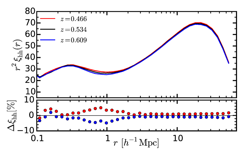
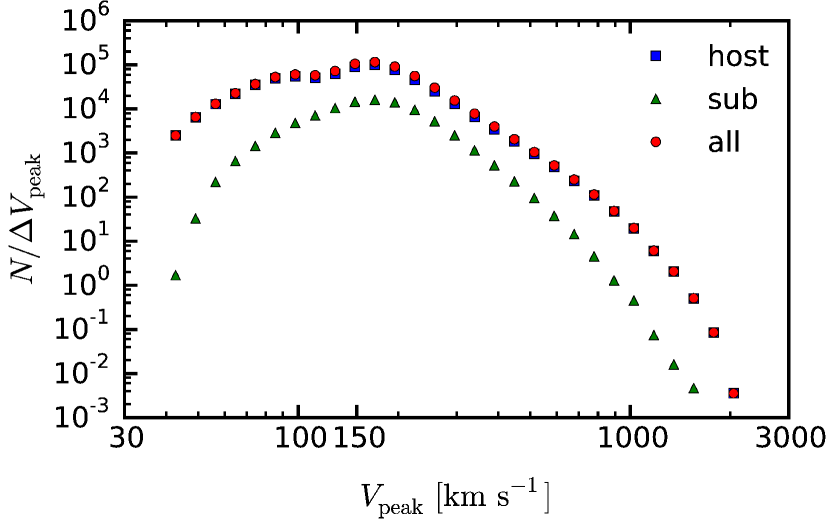
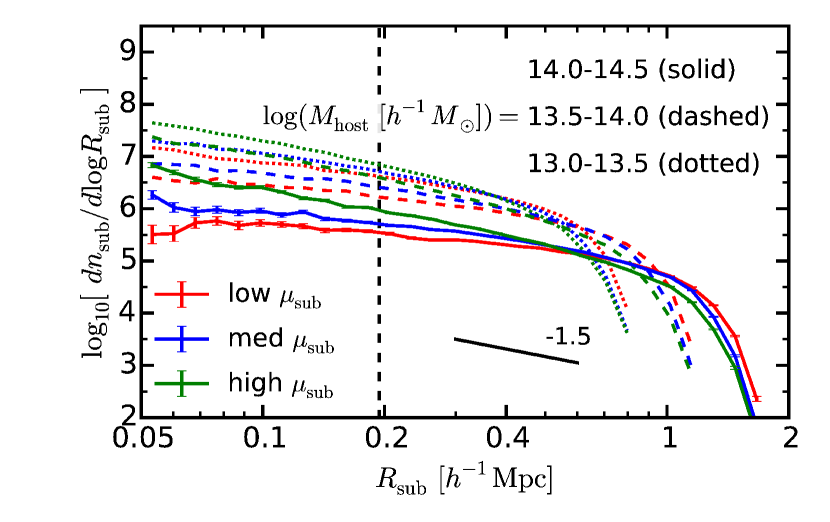
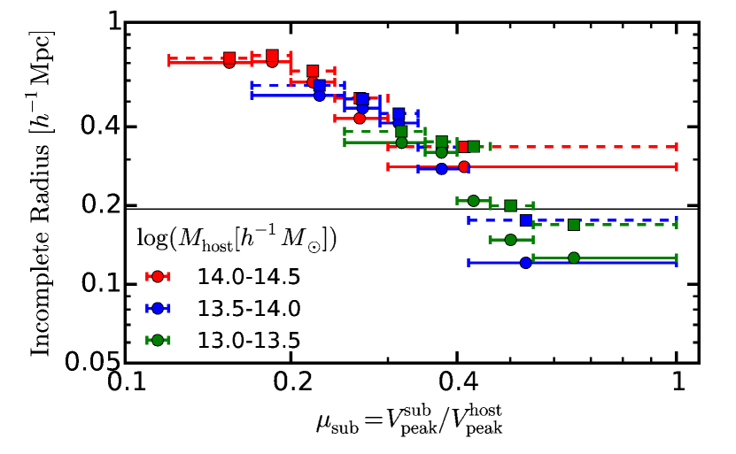
Appendix B Impact of the scatter in the relation for the age-matching model
To study the impact of the assembly bias effect, we adopt the age-matching model where we reorganize the relation between subhalo age and galaxy color at fixed stellar mass rather than at fixed halo mass (or ). This is because we can perform rank-order matching only against observable quantities. However, because our study operates in the very steep end of the stellar mass function, we must verify that our results do not depend on the stellar mass bin width when performing age-matching. In H13, the authors report that their analysis is insensitive to a stellar-mass bin width of . In this appendix, we perform a similar exercise to H13 for our extreme age-matching model (see section 6.3). In the following, we demonstrate that our results are insensitive to our fiducial bin width of . However, we also show that the choice of a fiducial bin width needs to take into consideration the scatter (in our case ).
We perform a test in which we consider the extreme age-matching model in section 6.3 but we reshuffle with respect to rather than . In addition, we test how the results vary if we use a different bin width. Figure 17 demonstrates that our results are insensitive to this change in bin width ( (blue) and (cyan)). We have also checked that our mean halo masses and satellite fractions are unchanged when going from to .
Nevertheless, figure 17 shows a clear difference between the simple abundance matching (‘AbM’, red) and the extreme age matching results (‘AgM-’, blue or cyan). In fact, the mean halo mass and the satellite fraction for the AbM (AgM-) models are (13.551), and (9.12%), respectively. We argue that this difference originates from the non-zero scatter in the relation in the abundance matching. In performing the extreme age-matching model with , CMASS galaxies with larger at fixed stellar mass are likely to have larger .
Our argument is confirmed by figure 18 where we perform the same exercise but we set . In this case, we find that our clustering prediction becomes stable with bin widths smaller than , and that AbM result is similar to the AgM- one (compare red with magenta lines). In figure 18, we also display the AgM model with a variety of halo-age indicators (see section 6.3). The halos masses of the blue, green and cyan curves are very similar (). Hence, differences in the clustering for the blue, green and cyan curves are a consequence of assembly bias effects.
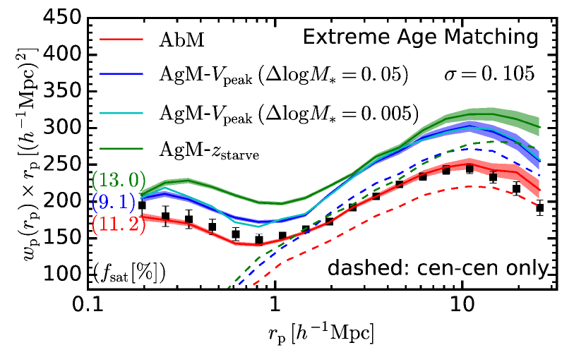
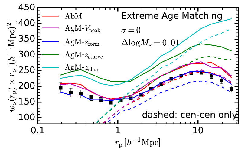
References
- Ahn et al. (2014) Ahn C. P., et al., 2014, ApJS, 211, 17
- Aihara et al. (2011) Aihara H., et al., 2011, ApJS, 193, 29
- Alam et al. (2015) Alam S., et al., 2015, preprint, (arXiv:1501.00963)
- Anderson et al. (2014) Anderson L., et al., 2014, Monthly Notices of the Royal Astronomical Society, 441, 24
- Baldry et al. (2008) Baldry I. K., Glazebrook K., Driver S. P., 2008, Monthly Notices of the Royal Astronomical Society, 388, 945
- Behroozi et al. (2010) Behroozi P. S., Conroy C., Wechsler R. H., 2010, ApJ, 717, 379
- Behroozi et al. (2013a) Behroozi P. S., Wechsler R. H., Wu H.-Y., 2013a, The Astrophysical Journal, 762, 109
- Behroozi et al. (2013b) Behroozi P. S., Wechsler R. H., Wu H.-Y., Busha M. T., Klypin A. A., Primack J. R., 2013b, The Astrophysical Journal, 763, 18
- Benson (2012) Benson A. J., 2012, New Astronomy, 17, 175
- Berlind & Weinberg (2002) Berlind A. A., Weinberg D. H., 2002, ApJ, 575, 587
- Beutler et al. (2014a) Beutler F., et al., 2014a, Monthly Notices of the Royal Astronomical Society, 443, 1065
- Beutler et al. (2014b) Beutler F., et al., 2014b, Monthly Notices of the Royal Astronomical Society, 444, 3501
- Bolton et al. (2012) Bolton A. S., et al., 2012, The Astronomical Journal, 144, 144
- Bundy et al. (2010) Bundy K., et al., 2010, ApJ, 719, 1969
- Bundy et al. (2015) Bundy K., et al., 2015, ApJS, 221, 15
- Carlson & White (2010) Carlson J., White M., 2010, ApJS, 190, 311
- Chabrier (2003) Chabrier G., 2003, PASP, 115, 763
- Coil et al. (2011) Coil A. L., et al., 2011, ApJ, 741, 8
- Conroy et al. (2006) Conroy C., Wechsler R. H., Kravtsov A. V., 2006, ApJ, 647, 201
- Coupon et al. (2015) Coupon J., et al., 2015, Monthly Notices of the Royal Astronomical Society, 449, 1352
- Croton et al. (2006) Croton D. J., et al., 2006, Monthly Notices of the Royal Astronomical Society, 365, 11
- Dalal et al. (2008) Dalal N., White M., Bond J. R., Shirokov A., 2008, Astrophysical Journal, 687, 12
- Davis & Peebles (1983) Davis M., Peebles P. J. E., 1983, ApJL, 267, 465
- Dawson et al. (2013) Dawson K. S., et al., 2013, The Astronomical Journal, 145, 10
- Dekel & Birnboim (2006) Dekel A., Birnboim Y., 2006, Monthly Notices of the Royal Astronomical Society, 368, 2
- Eisenstein et al. (2011) Eisenstein D. J., et al., 2011, The Astronomical Journal, 142, 72
- Fèvre et al. (2015) Fèvre O. L., et al., 2015, Astronomy & Astrophysics, 576, A79
- Fraser-McKelvie et al. (2014) Fraser-McKelvie A., Brown M. J. I., Pimbblet K. A., 2014, Monthly Notices of the Royal Astronomical Society: Letters, 444, L63
- Fukugita et al. (1996) Fukugita M., Ichikawa T., Gunn J. E., Doi M., Shimasaku K., Schneider D. P., 1996, The Astronomical Journal, 111, 1748
- Gao & White (2007) Gao L., White S. D. M., 2007, Monthly Notices of the Royal Astronomical Society: Letters, 377, L5
- Gao et al. (2005) Gao L., Springel V., White S. D. M., 2005, Monthly Notices of the Royal Astronomical Society: Letters, 363, L66
- Gunn et al. (1998) Gunn J. E., et al., 1998, The Astronomical Journal, 116, 3040
- Gunn et al. (2006) Gunn J. E., et al., 2006, AJ, 131, 2332
- Guo et al. (2013) Guo H., et al., 2013, ApJ, 767, 122
- Guo et al. (2014) Guo H., et al., 2014, Monthly Notices of the Royal Astronomical Society, 446, 578
- Guo et al. (2016) Guo H., et al., 2016, MNRAS,
- Guzzo et al. (2014) Guzzo L., et al., 2014, Astronomy & Astrophysics, 566, A108
- Hartlap et al. (2007) Hartlap J., Simon P., Schneider P., 2007, Astronomy and Astrophysics, 464, 399
- Hearin et al. (2013a) Hearin A. P., Zentner A. R., Berlind A. A., Newman J. A., 2013a, Monthly Notices of the Royal Astronomical Society, 433, 659
- Hearin et al. (2013b) Hearin A. P., Zentner A. R., Berlind A. A., Newman J. A., 2013b, Monthly Notices of the Royal Astronomical Society, 433, 659
- Hearin et al. (2014a) Hearin A. P., Watson D. F., van den Bosch F. C., 2014a, preprint, (arXiv:1404.6524)
- Hearin et al. (2014b) Hearin A. P., Watson D. F., Becker M. R., Reyes R., Berlind A. A., Zentner A. R., 2014b, Monthly Notices of the Royal Astronomical Society, 444, 729
- Ishiyama et al. (2014) Ishiyama T., Enoki M., Kobayashi M. A. R., Makiya R., Nagashima M., Oogi T., 2014, preprint, (arXiv:1412.2860)
- Jing et al. (2007) Jing Y. P., Suto Y., Mo H. J., 2007, ApJ, 657, 664
- Kitaura et al. (2013) Kitaura F.-S., Yepes G., Prada F., 2013, Monthly Notices of the Royal Astronomical Society: Letters, 439, L21
- Knebe et al. (2011) Knebe A., et al., 2011, Monthly Notices of the Royal Astronomical Society, 415, 2293
- Komatsu et al. (2009) Komatsu E., et al., 2009, The Astrophysical Journal Supplement Series, 180, 330–376
- Kravtsov et al. (2004) Kravtsov A. V., Berlind A. A., Wechsler R. H., Klypin A. A., Gottlober S., Allgood B., Primack J. R., 2004, ApJ, 609, 35
- Landy & Szalay (1993) Landy S. D., Szalay A. S., 1993, ApJL, 412, 64
- Lawrence et al. (2007) Lawrence A., et al., 2007, MNRAS, 379, 1599
- Leauthaud et al. (2011) Leauthaud A., et al., 2011, ApJ, 744, 159
- Leauthaud et al. (2015) Leauthaud A., et al., 2015, preprint, (arXiv:1507.04752)
- Lewis & Bridle (2002) Lewis A., Bridle S., 2002, Physical Review D, 66
- Li et al. (2008) Li Y., Mo H. J., Gao L., 2008, Monthly Notices of the Royal Astronomical Society, 389, 1419
- Lilly et al. (2007) Lilly S. J., et al., 2007, The Astrophysical Journal Supplement, 172, 70
- Lim et al. (2015) Lim S. H., Mo H. J., Wang H., Yang X., 2015, preprint, (arXiv:1502.01256)
- Lin et al. (2015) Lin Y.-T., Mandelbaum R., Huang Y.-H., Huang H.-J., Dalal N., Diemer B., Jian H.-Y., Kravtsov A., 2015, preprint, (arXiv:1504.07632)
- Liu et al. (2012) Liu F. S., Mao S., Meng X. M., 2012, Monthly Notices of the Royal Astronomical Society, 423, 422
- Lu et al. (2014) Lu Y., et al., 2014, ApJ, 795, 123
- Mandelbaum et al. (2006) Mandelbaum R., Seljak U., Kauffmann G., Hirata C. M., Brinkmann J., 2006, Monthly Notices of the Royal Astronomical Society, 368, 715
- Mandelbaum et al. (2015) Mandelbaum R., Wang W., Zu Y., White S., Henriques B., More S., 2015, preprint, (arXiv:1509.06762)
- Manera et al. (2012) Manera M., et al., 2012, Monthly Notices of the Royal Astronomical Society, 428, 1036
- Maraston et al. (2009) Maraston C., Strömbäck G., Thomas D., Wake D. A., Nichol R. C., 2009, Monthly Notices of the Royal Astronomical Society: Letters, 394, L107
- Masaki et al. (2013) Masaki S., Lin Y.-T., Yoshida N., 2013, Monthly Notices of the Royal Astronomical Society, 436, 2286
- Masters et al. (2011) Masters K. L., et al., 2011, Monthly Notices of the Royal Astronomical Society, 418, 1055
- McDonald et al. (2012) McDonald M., et al., 2012, Nature, 488, 349
- Miyatake et al. (2013) Miyatake H., et al., 2013, preprint, (arXiv:1311.1480)
- Miyatake et al. (2015) Miyatake H., More S., Takada M., Spergel D. N., Mandelbaum R., Rykoff E. S., Rozo E., 2015, preprint, (arXiv:1506.06135)
- Mo et al. (2010) Mo H., van den Bosch F. C., White S., 2010, Galaxy Formation and Evolution
- Montero-Dorta et al. (2014) Montero-Dorta A. D., et al., 2014, preprint, (arXiv:1410.5854)
- More (2013) More S., 2013, ApJ, 777, L26
- More et al. (2014) More S., Miyatake H., Mandelbaum R., Takada M., Spergel D., Brownstein J., Schneider D. P., 2014,
- Moster et al. (2010) Moster B. P., Somerville R. S., Maulbetsch C., van den Bosch F. C., Macciò A. V., Naab T., Oser L., 2010, ApJ, 710, 903
- Moustakas et al. (2013) Moustakas J., et al., 2013, ApJ, 767, 50
- Newman et al. (2013) Newman J. A., et al., 2013, ApJS, 208, 5
- Nuza et al. (2013) Nuza S. E., et al., 2013, Monthly Notices of the Royal Astronomical Society, 432, 743
- Oke & Gunn (1983) Oke J. B., Gunn J. E., 1983, ApJ, 266, 713
- Onions et al. (2012) Onions J., et al., 2012, Monthly Notices of the Royal Astronomical Society, 423, 1200–1214
- Prada et al. (2012) Prada F., Klypin A. A., Cuesta A. J., Betancort-Rijo J. E., Primack J., 2012, Monthly Notices of the Royal Astronomical Society, 423, 3018
- Reddick et al. (2013) Reddick R. M., Wechsler R. H., Tinker J. L., Behroozi P. S., 2013, ApJ, 771, 30
- Reid et al. (2014) Reid B. A., Seo H.-J., Leauthaud A., Tinker J. L., White M., 2014, Monthly Notices of the Royal Astronomical Society, 444, 476
- Reid et al. (2016) Reid B., et al., 2016, MNRAS, 455, 1553
- Riebe et al. (2013) Riebe K., et al., 2013, Astronomische Nachrichten, 334, 691
- Rodríguez-Torres et al. (2015) Rodríguez-Torres S. A., et al., 2015, preprint, (arXiv:1509.06404)
- Ross et al. (2013) Ross A. J., et al., 2013, Monthly Notices of the Royal Astronomical Society, 437, 1109
- Saito et al. (2011) Saito S., Takada M., Taruya A., 2011, Physical Review D, 83
- Saito et al. (2014) Saito S., Baldauf T., Vlah Z., Seljak U., Okumura T., McDonald P., 2014, Physical Review D, 90
- Samushia et al. (2014) Samushia L., et al., 2014, Monthly Notices of the Royal Astronomical Society, 439, 3504
- Schlegel et al. (1998) Schlegel D. J., Finkbeiner D. P., Davis M., 1998, ApJ, 500, 525
- Skillman et al. (2014) Skillman S. W., Warren M. S., Turk M. J., Wechsler R. H., Holz D. E., Sutter P. M., 2014,
- Smee et al. (2013) Smee S. A., et al., 2013, The Astronomical Journal, 146, 32
- Smith (2012) Smith R. E., 2012, Monthly Notices of the Royal Astronomical Society, 426, 531
- Tinker et al. (2011) Tinker J. L., et al., 2011, ApJ, 745, 16
- Tinker et al. (2012) Tinker J. L., George M. R., Leauthaud A., Bundy K., Finoguenov A., Massey R., Rhodes J., Wechsler R. H., 2012, ApJ, 755, L5
- Tinker et al. (2013) Tinker J. L., Leauthaud A., Bundy K., George M. R., Behroozi P., Massey R., Rhodes J., Wechsler R. H., 2013, ApJ, 778, 93
- Tojeiro et al. (2014) Tojeiro R., et al., 2014, Monthly Notices of the Royal Astronomical Society, 440, 2222
- Vale & Ostriker (2004) Vale A., Ostriker J. P., 2004, Monthly Notices of the Royal Astronomical Society, 353, 189
- Watson et al. (2014) Watson D. F., et al., 2014, Monthly Notices of the Royal Astronomical Society, 446, 651
- Wechsler et al. (2006) Wechsler R. H., Zentner A. R., Bullock J. S., Kravtsov A. V., Allgood B., 2006, ApJ, 652, 71
- White et al. (2011) White M., et al., 2011, ApJ, 728, 126
- White et al. (2013) White M., Tinker J. L., McBride C. K., 2013, Monthly Notices of the Royal Astronomical Society, 437, 2594
- Zehavi et al. (2005) Zehavi I., et al., 2005, ApJ, 630, 1
- Zehavi et al. (2011) Zehavi I., et al., 2011, ApJ, 736, 59
- Zentner et al. (2014) Zentner A. R., Hearin A. P., van den Bosch F. C., 2014, Monthly Notices of the Royal Astronomical Society, 443, 3044
- Zhao et al. (2013) Zhao G.-B., et al., 2013, Monthly Notices of the Royal Astronomical Society, 436, 2038
- Zheng et al. (2005) Zheng Z., et al., 2005, ApJ, 633, 791
- Zu & Mandelbaum (2015) Zu Y., Mandelbaum R., 2015, preprint, (arXiv:1505.02781)
- van den Bosch et al. (2013) van den Bosch F. C., More S., Cacciato M., Mo H., Yang X., 2013, MNRAS, 430, 725