Radiation from a Relativistic Poynting Jet: some general considerations

Abstract

We provide estimates for the flux and maximum frequency of radiation produced when the magnetic field in a relativistic, highly magnetized, jet is dissipated and particles are accelerated using general considerations. We also provide limits on the jet Lorentz factor and magnetization parameter from the observed flux. Furthermore, using the Lorentz invariance of scalar quantities produced with electromagnetic tensor, we provide constraints on particle acceleration, and general features of the emergent radiation. We find that the spectrum below the peak softens with decreasing frequency. This spectral feature might be one way of identifying a magnetic jet.

1 Introduction

Relativistic jets where the energy is transported outward by Poynting flux ($\vec{E}$x$\vec{B}$) have been invoked for many energetic outflows in astrophysical systems such as pulsars, quasars, micro-quasars and gamma-ray bursts (GRB). There is a vast peer reviewed literature on this topic e.g., Michel (1969), Blandford & Znajek (1977) Blandford & Payne (1982), Kennel and Coroniti (1884), Begelman, et al. (1984), Coroniti (1990), Mészáros & Rees (1997), Lyubarsky & Kirk (2001), de Gouveia dal Pino & Lazarian (2005), Drenkhahn & Spruit (2002), Lovelace et al. (2002), Kulsrud (2005), Giannios & Spruit (2006), Komissarov et al. (2007), Tchekhovskoy et al. (2008), Metzger et al. (2011), Cerutti et al. (2012).

The radiation is produced in these systems as a result of magnetic field dissipation (referred to as reconnection, a generic phrase, which we will be using throughout this article), where particles are accelerated either via parallel electric field or first order Fermi process in converging flows, and they then emit photons via the synchrotron process. Radiation could also be produced in shocks internal to the jet or when the jet interacts with the surrounding medium via a shock and transfers a fraction of its energy to particles in the external medium We do not consider the latter process in this paper.

Magnetic reconnection is a complex and poorly understood process despite the work of numerous people on this problem for the last more than 50 years, e.g. Dungey (1953), Sweet (1958), Parker (1957), Petschek (1964), Syrovatskii (1981), Biskamp (1986), Yamada et al. (1997), Kulsrud (1998), Uzdensky & Kulsrud (2000), Birn et al.(2001), Drake (2006), Samtaney et al. (2009), Zweibel & Yamada (2009). Does this mean that we are doomed in our effort to understand those astrophysical systems where Poynting jets play an important role until a predictive theory for reconnections is developed? The answer depends on what it is that we want to understand about these systems. If we are interested in the general, global, properties then the fine details of the reconnection process might not matter. A basic understanding can be obtained from certain Lorentz invariant functions of electromagnetic tensor and conservation laws. The goal of this paper is thus modest, and highly restricted in this sense, i.e. to try to provide some constraints on Poynting jet parameters (without having to rely on a particular reconnection model) so that magnetic dissipation can explain some broad aspects of the data such as the efficiency for converting magnetic energy to radiation and the general shape of the emergent spectrum. In a recent paper Beniamini & Piran (2014) have provided constraints on a Poynting jet model for GRBs. Their general approach and results are very different from the one we pursue here.

In section 2 we provide a few general properties of Poynting jet. We estimate the maximum energy electrons could achieve in reconnection, and the shape of emergent spectrum also in §2.

2 Poynting jet: a few general considerations

Figure 1 provides a schematic sketch of the system we are considering. The magnetic fields of a relativistic Poynting jet undergo dissipation at some radius $R$ and a number of current sheets form within the causally connected region of the jet of comoving size $R/\Gamma$ ($R/\Gamma^{2}$ in lab frame) and efficiently convert the magnetic energy to particle energy and radiation. Within any current sheet there are likely to be a number of different regions where particles are accelerated, and within a space of size $R/\Gamma$ there are obviously many more. These acceleration regions are usually associated with X-points — located in between plasmoids or magnetic islands that form due to tearing instability – where the magnetic field vanishes in absence of a guide field and where the electric field can accelerate particles, or with converging flows where particle acceleration takes place via first order Fermi process. Regions where particles are accelerated will be referred to as PASs (particle acceleration sites). Some general considerations regarding particle acceleration in an individual PAS is discussed in §2.1. The maximum Lorentz factor (LF) of particles in PASs is determined by a combination of electric field strength and radiative losses in addition to energy conservation (§2.1). While outside PASs, particles lose energy to radiation and any acceleration they experience is negligible. The particle distribution function inside PASs is not determined in this paper and is taken to be a hard powerlaw function as per numerical simulations (Zenitani & Hoshino 2001; Jaroschek et al. 2004; Sironi & Spitkovsky 2011, 2014; Guo et al. 2014). However, the distribution function outside PASs is determined by solving an appropriate set of equations (§2.2). Synchrotron radiation emanating from PASs and outside PASs is considered in §2.3. In §2.4 we provide an estimate for distance from the center where Poynting jet is likely dissipated and the number of current sheets in the causally connected region for an efficient conversion of magnetic energy to radiation.

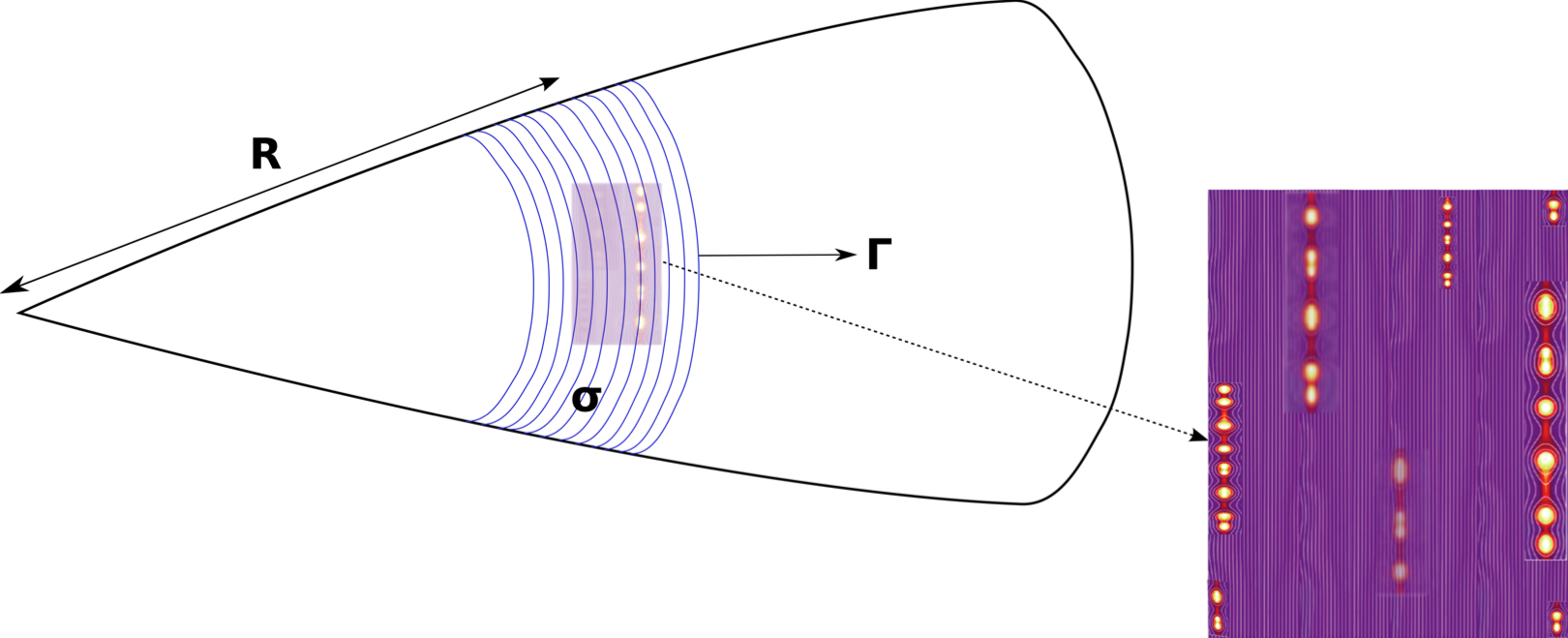
Figure 1: A schematic sketch of a Poynting jet and multiple reconnection zones within the causally connected region of comoving size $R/\Gamma$. Each reconnection zone has a number of particle-acceleration-sites (PASs), which are either regions between bright spots or plasmoids where magnetic field is small and particles are accelerated by electric fields or regions of converging flows where particles are accelerated by the Fermi process. The reconnection zones shown in this figure are artistic renditions of numerical simulations of Hesse & Zenitani (2007).

Let us consider a Poynting jet with magnetization parameter $\sigma$, Lorentz factor (LF) $\Gamma$, and isotropic equivalent luminosity $L$. The dissipation of magnetic field takes place when the jet is at radius R, and that is also roughly the radius where radiation is produced. The plasma is sufficiently cold before magnetic reconnections so that the thermal pressure of particles can be ignored.

The magnetic field in the jet comoving frame is $B^{\prime}_{0}$ — all physical quantities in the jet comoving frame are denoted by a prime and observer frame variables are un-primed — which is related to jet luminosity as

$$L=B^{\prime 2}_{0}\Gamma^{2}R^{2}c\quad\Longrightarrow\quad B^{\prime}_{0}={(L/c)^{1/2}\over\Gamma R}=(58\ {\rm G}){L_{48}^{1/2}\over\Gamma_{2}R_{15}}$$ (1)

provided that $\sigma>1$; we are using the convenient notation $X_{n}\equiv X/10^{n}$.

We adopt the standard model that charged particles are accelerated in reconnection layers where magnetic field dissipation takes place. The accelerated electrons with “thermal” LF $\gamma^{\prime}_{e}$ emit synchrotron photons of frequency less than or equal to $\nu$ (in the observer frame) which is given by

$$\nu\approx{qB^{\prime}_{0}\gamma^{\prime 2}_{e}\Gamma\over 2\pi m_{e}c(1+z)},$$ (2)

where $q$ and $m_{e}$ are electron charge and mass, and $z$ is the redshift of the object. An upper limit to $\gamma^{\prime}_{e}$ can be obtained from energy conservation, i.e. the energy in accelerated particles cannot exceed the energy in magnetic field. This condition gives

$$n^{\prime}_{e}\gamma^{\prime}_{max}m_{e}c^{2}\lower 2.0pt\hbox{$\,\buildrel\scriptstyle<\over{\scriptstyle\sim}\,$}{B^{\prime 2}_{0}\over 8\pi}\Longrightarrow\gamma^{\prime}_{max}\lower 2.0pt\hbox{$\,\buildrel\scriptstyle<\over{\scriptstyle\sim}\,$}(m_{p}/m_{e})\sigma,$$ (3)

where $n^{\prime}_{e}$ is electron number density in the jet comoving frame, and

$$\sigma\equiv B^{\prime 2}_{0}/(8\pi n_{e}^{\prime}m_{p}c^{2})$$ (4)

is jet magnetization parameter. The reason that equation (3) gives the maximum electron LF and not the average LF is because electrons accelerated in current sheets have a power-law distribution function ($dn_{e}/d\gamma_{e}\propto\gamma_{e}^{-p}$) with $p<2$, and therefore most of the electron “thermal” energy is carried by the highest energy electrons; numerical simulations find $p<2$ when the region where the reconnection takes place is strongly magnetized, $\sigma\lower 2.0pt\hbox{$\,\buildrel\scriptstyle>\over{\scriptstyle\sim}\,$}$ a few, and when the reconnection layer is sufficiently large in size (e.g. Romanova & Lovelace 1992; Zenitani & Hoshino 2001; Sironi & Spitkovsky 2014; Bessho & Bhattacharjee 2012, Werner et al. 2014, Guo et al. 2014). Making use of equations 1 & 3 for magnetic field strength and electron LF, we obtain an expression for the maximum synchrotron frequency

$$\nu_{max}^{syn}\sim{qL^{1/2}\sigma^{2}(m_{p}/m_{e})^{2}\over 2\pi m_{e}c^{3/2}R(1+z)}=(2.2\times 10^{2}{\rm eV}){\sigma^{2}L_{48}^{1/2}\over R_{15}(1+z)}.$$ (5)

A more accurate estimate for $\nu_{max}^{syn}$ that takes into account radiative losses are presented in §2.1. The synchrotron photons will be inverse-Compton (IC) scattered to higher energies by electrons producing these photons, and the maximum IC photon energy in observer frame is the smaller of $m_{e}c^{2}\gamma^{\prime}_{e}\Gamma/(1+z)$ and $\sim\nu\gamma^{\prime 2}_{max}$.

The specific flux at frequency $\nu$, i.e. flux per unit frequency, in the observer frame is

$$f_{\nu}\approx\left[{q^{3}B^{\prime}_{0}\Gamma N_{e}\over m_{e}c^{2}}\right]{1+z\over 4\pi d_{L}^{2}},$$ (6)

where $N_{e}$ is the total number of electrons (isotropic equivalent) in the causally connected part of the jet with thermal LF $\geq\gamma_{e}$, and $d_{L}$ is the luminosity distance to the source. We can calculate the number of electrons needed to produce a given observed flux by combining equations (1)–(6):

$$N_{e}\approx 1.2\times 10^{49}f_{\nu,mJy}L_{48}^{-1/2}R_{15}d_{L,28}^{2}(1+z)^{-1},$$ (7)

The optical depth of these electrons to Thomson scattering is,

$$\tau_{T}\approx{\sigma_{T}N_{e}\over 4\pi R^{2}}=8\times 10^{-7}\,f_{\nu,mJy}L_{48}^{-1/2}R_{15}^{-1}d_{L,28}^{2}(1+z)^{-1},$$ (8)

and their “thermal” LF and kinetic energy luminosity they carry are

$$\gamma^{\prime}_{e}\approx\left[{2\pi m_{e}\nu Rc^{3/2}\over qL^{1/2}(1+z)^{-1}}\right]^{1/2}=4\times 10^{3}{[R_{15}\nu_{kev}(1+z)]^{1/2}\over L_{48}^{1/4}},$$ (9)

$$L_{e} \approx {N_{e}m_{e}c^{3}\gamma_{e}\Gamma\over(R/\Gamma^{2})}$$ (10)

$$= (1.2\times 10^{42}{\rm erg\,s^{-1}}){\Gamma^{3}f_{\nu,mJy}R_{15}^{1/2}d_{L,28}^{2}\nu_{keV}^{1/2}\over L_{48}^{3/4}(1+z)^{1/2}},$$

where $\nu_{keV}$ is photon frequency (in units of 1 keV) for which the observed specific flux is $f_{\nu,mJy}$. Considering that the energy carried by electrons cannot exceed the energy in magnetic fields for a Poynting jet, we find

$$L_{e}/L\lower 2.0pt\hbox{$\,\buildrel\scriptstyle<\over{\scriptstyle\sim}\,$}1\quad\Longrightarrow\quad\Gamma\lower 2.0pt\hbox{$\,\buildrel\scriptstyle<\over{\scriptstyle\sim}\,$}90\;{L_{48}^{7/12}(1+z)^{1/6}\over f_{\nu,mJy}^{1/3}R_{15}^{1/6}d_{L,28}^{2/3}\nu_{keV}^{1/6}}.$$ (11)

The reason for the approximate inequality sign in the above equation is because magnetic fields of a Poynting jet could be compressed by a factor a few and thus $L_{e}$ could in principle exceed $L$ by order unity.

If we consider that there are $\eta_{p}$ protons for every electron that radiates at frequency $\nu$, then the kinetic energy luminosity carried by cold protons is

$$L_{p}\approx{N_{e}\eta_{p}m_{p}c^{3}\Gamma\over(R/\Gamma^{2})}\approx(5\times 10^{41}{\rm erg\,s^{-1}}){\Gamma^{3}\eta_{p}f_{\nu,mJy}d_{L,28}^{2}\over L_{48}^{1/2}(1+z)}.$$ (12)

Therefore, the magnetization parameter for the jet at location where jet magnetic energy is dissipated and radiation is produced is given by

$$\sigma(R)\approx{L\over L_{p}}\approx{2\times 10^{6}\over\eta_{p}\Gamma^{3}}f_{\nu,mJy}^{-1}L_{48}^{3/2}d_{L,28}^{-2}(1+z).$$ (13)

If 10% of electrons in the jet are accelerated. i.e. $\eta_{p}=10$, and $\Gamma=20$, then $\sigma(R)\approx 25$. And that means that the magnetization parameter at the let launching site where $\Gamma\sim 1$ is $\sigma_{0}\approx\Gamma(R)\sigma(R)\sim 500$.

2.1 Particle acceleration in current sheets

Consider an electron undergoing acceleration in a reconnection region where the electric field is $\vec{E}^{\prime}$, and the magnetic field is $\vec{B}^{\prime}$. In the absence of a guide field, the magnetic field vanishes at the X-point, and far away from it its magnitude is $B_{0}^{\prime}$, but otherwise at this stage we place no further constraint on the electric and magnetic fields. The electron starting from some place in the vicinity of the X-point is accelerated, and as it moves away it finds the strength of the magnetic field increasing. At some point when the magnetic field becomes sufficiently strong, which will be quantified shortly, the acceleration ceases if $\vec{E}^{\prime}\cdot\vec{B}^{\prime}=0$. However, even well before this happens, the electron could stop accelerating due to radiative losses which will determine its terminal Lorentz factor. We consider this interplay between acceleration and radiative losses to determine maximum electron LF.

It is best to view the motion of a particle acted upon by $\vec{E}^{\prime}$ and $\vec{B}^{\prime}$ from a frame where the fields point in the same direction (which is always possible except when $|\vec{E}^{\prime}|=|\vec{B}^{\prime}|$ and the two fields are exactly perpendicular to each other). This special frame where $\vec{E}^{\prime\prime}\parallel\vec{B}^{\prime\prime}$ will be referred to as the AF frame (Aligned Fields frame). There are two quadratic Lorentz invariant functions of $\vec{E}^{\prime}$ and $\vec{B}^{\prime}$:

$$I_{1} = -\epsilon_{\alpha\beta\gamma\delta}F^{\alpha\beta}F^{\gamma\delta}/8=\vec{E}^{\prime}\cdot\vec{B}^{\prime}\quad{\it and}$$

$$I_{2} = -F^{\alpha\beta}F_{\alpha\beta}/2=E^{\prime 2}-B^{\prime 2},$$ (14)

where $F_{\alpha\beta}$ is the electromagnetic tensor (anti-symmetric 2-form). Since $\vec{E^{\prime}}\cdot\vec{B^{\prime}}$ is Lorentz invariant, if there is a non-zero component of magnetic field in the direction of the electric field in one inertial frame, there will be a non-zero component in all inertial frames. However, the component of magnetic field perpendicular to the electric field can be made to vanish by frame transformation if $E^{\prime 2}-B^{\prime 2}>0$, or the electric field perpendicular to magnetic field can be transformed away in an appropriate frame when $E^{\prime 2}-B^{\prime 2}<0$. The point is that there exists an inertial frame (AF) where the transformed electric and magnetic fields are parallel, and the motion of the electron is the AF frame is as simple as can be — the electron momentum parallel to the fields increases linearly with time (if the electric field is non-zero in this frame), and the perpendicular component of momentum has a constant magnitude (time independent) and it rotates about the magnetic field at a constant rate.

The simplest way to get to the AF frame is by a Lorentz boost in the direction $\vec{E}^{\prime}\times\vec{B}^{\prime}$; if $\vec{E}^{\prime}\times\vec{B}^{\prime}=0$, then obviously no Lorentz transformation is needed as we are already in a frame where the two fields are either parallel or one of them is zero. A straightforward Lorentz transformation algebra shows that the speed of the Lorentz boost required so that the fields are parallel in the new frame is

$$\beta_{LT}={(1+\epsilon^{2})-\left[(1-\epsilon^{2})^{2}+4\epsilon^{2}\cos^{2}\theta^{\prime}\right]^{1/2}\over 2\epsilon\sin\theta^{\prime}}$$ (15)

where

$$\epsilon\equiv{E^{\prime}\over B^{\prime}},\quad\cos\theta^{\prime}={\vec{E}^{\prime}\cdot\vec{B}^{\prime}\over|\vec{E}^{\prime}||\vec{B}^{\prime}|}.$$ (16)

Figure 2 shows the LF of needed boost as a function of $\epsilon$ for a few different values of $\theta^{\prime}$; a simple analytical expression for $\epsilon\gg 1$ and $\epsilon\ll 1$ is

$$\beta_{LT}\approx\min\left\{\epsilon,\epsilon^{-1}\right\}\sin\theta^{\prime},$$ (17)

which turns out to be exact (as opposed to approximate) for all values of $\epsilon$ for the special case of $\theta^{\prime}=\pi/2$.

Figure 2: The Lorentz factor of the inertial frame (wrt jet rest-frame) in which the electric and magnetic fields in some region of current sheet are parallel to each other is shown in the upper panel as a function of $\epsilon\equiv E^{\prime}/B^{\prime}$; $\Gamma_{LT}\equiv(1-\beta_{LT}^{2})^{-1/2}$, where $\beta_{LT}$ is given by equation (15). The three different curves correspond to three different angles ($\theta^{\prime}$) between electric and magnetic fields; $\theta^{\prime}=70^{o}$ (dashed curve), $80^{o}$ (dotted line), and $90^{o}$ (solid line). Note that $\Gamma_{LT}\sim 1$ except when electric field is almost exactly perpendicular to the magnetic field and the strengths of these fields are about the same. This makes it rather easy to carry out calculations in the AF frame where $\vec{E}^{\prime\prime}\parallel\vec{B}^{\prime\prime}$ and transform variables back to the jet comoving frame. The lower panel shows the angle (measured in the jet comoving frame in degrees) by which the electric field direction is rotated in the AF frame for three different values of $\theta^{\prime}$ which are same as in the upper panel; when the electric field vanishes is the AF frame then the angle is the rotation for magnetic field plus $\pi/2$.

The electric field in the new frame follows from the two Lorentz invariant quantities mentioned above and is given by

$$E^{\prime\prime 2}={I_{2}+\sqrt{4I_{1}^{2}+I_{2}^{2}}\over 2},$$ (18)

and the magnetic field is

$$B^{\prime\prime}={I_{1}\over E^{\prime\prime}},$$ (19)

where $I_{1}$ and $I_{2}$ are defined in equation (14). The angle between the aligned electro-magnetic field in the AF frame and the electric field in the jet frame can be easily calculated and is

$$\cos\theta^{\prime}_{E}={(\epsilon-\beta_{LT}\sin\theta^{\prime})\over\sqrt{\epsilon^{2}+\beta_{LT}^{2}-2\epsilon\beta_{LT}\sin\theta^{\prime}}},$$ (20)

The lower panel of Figure 2 shows $\theta^{\prime}_{E}$ as a function of $\epsilon$ for a few different values of $\theta^{\prime}$.

With these results in hand, we are ready to describe particle acceleration in a current sheet. Consider a charged particle in the vicinity of the X-point where $E^{\prime}\gg B^{\prime}$. We can transform away the perpendicular component of the magnetic field by going to the AF frame, and in this frame the particle Lorentz factor $\gamma_{e}^{\prime\prime}$ (the double prime emphasizes that we are in a different inertial frame, and not the jet comoving frame) increases as $qE^{\prime\prime}t^{\prime\prime}/(m_{e}c^{2})$, which can be rewritten from the point of view of the jet frame as

$$\gamma^{\prime}_{e}\approx{q\epsilon_{0}B^{\prime}_{0}\ell^{\prime}\over m_{e}c^{2}},$$ (21)

where $\ell^{\prime}$ is the distance the electron has traveled along the direction of the electric field from its starting position in the jet comoving frame, and

$$\epsilon_{0}\equiv E^{\prime}/B^{\prime}_{0}.$$ (22)

As the electron travels further and further away from the X-point, it feels the strength of the magnetic field increase and at some point when $B^{\prime}$ becomes stronger than $E^{\prime}$ the electron is no longer accelerated (unless $\vec{E}^{\prime}\cdot\vec{B}^{\prime}\not=0$) and its momentum vector gyrates about the magnetic field and the LF oscillations and drifts slowly with time. This generic behavior can been in figure (3) where numerical result for particle motion in a current sheet is presented.

If the length of the region where $E^{\prime}>B^{\prime}$ is $\ell^{\prime}_{E}$, then the maximum LF of electron $\gamma^{\prime}_{max}\sim q\epsilon_{0}B^{\prime}_{0}\ell^{\prime}_{E}/(m_{e}c^{2})$; it should be noted that $\ell^{\prime}_{E}\lower 2.0pt\hbox{$\,\buildrel\scriptstyle\propto\over{\scriptstyle\sim}\,$}\epsilon_{0}$ for a magnetic field configuration where $B^{\prime}$ increases linearly with distance from the X-point, and thus $\gamma^{\prime}_{max}\lower 2.0pt\hbox{$\,\buildrel\scriptstyle\propto\over{\scriptstyle\sim}\,$}\epsilon_{0}^{2}$ (see e.g. Larrabee et al, 2003). However, two effects can substantially limit electron LF below this value. One of which is “global” energy conservation, which provides a limit for $\gamma^{\prime}_{max}$ as described by equation (3). And the other is radiative losses — synchrotron and inverse-Compton (IC) for systems of interest to us — that could restrict particle LF further. This is discussed below.

Figure 3: Acceleration of an electron in a current sheet is shown as a function of time in unit of $1/\omega_{c}$, where $\omega_{c}=qB^{\prime}_{0}/(m_{e}c)$ is Larmor frequency. The electric and magnetic field configurations in the current sheet are taken from Larrabee et al (2003), i.e. sheet lies in the x-y plane with the electric field pointing in the x-direction and has a constant magnitude $E^{\prime}=\epsilon_{0}B^{\prime}_{0}$, and the vector potential is ${\vec{A}}=[B^{\prime}_{0}(y^{2}-z^{2})/2\ell^{\prime}_{s}]\hat{z}$; we took $\epsilon_{0}=0.01$ and the length of the “sheet” $\ell^{\prime}_{s}\omega_{c}/c=5\times 10^{5}$ for this calculation. The particle started out in the $z=0$ plane with initial velocity of zero. The LF of the electron ($\gamma^{\prime}_{e}$) increases linearly with time as long as it is in the region where $E^{\prime}>B^{\prime}$ (which is for about 2x10${}^{4}\omega_{c}^{-1}$ for the parameters we have chosen for this calculation), and afterward when $B^{\prime}>E^{\prime}$ the acceleration ceases and the electron gyrates about the magnetic field. These results are entirely consistent with analytical calculations presented in this section.

Viewed from the AF frame where $\vec{E}^{\prime\prime}\parallel\vec{B}^{\prime\prime}$, the electron suffers radiative losses due to acceleration along the electric field direction, gyration about the magnetic field, and inverse-Compton scatterings. We evaluate each of these to determine the dominant loss mechanism, and its effect on $\gamma^{\prime}_{max}$. The energy loss rate is calculated by first assuming that the magnetic field lines are parallel, i.e. $\vec{B}^{\prime}\cdot\vec{\nabla}\vec{B}^{\prime}=0$, and the electric field is nearly uniform. This estimate is then improved by relaxing these assumptions and by considering the more realistic possibility that magnetic field lines have non-zero curvature, and that the electric field has spacial fluctuations in the acceleration region.

The power radiated due to particle acceleration along the electric field can be calculated using the Larmor’s formula. The momentum vector of the electron in the AF frame is nearly parallel to $\vec{E}^{\prime\prime}$ since it is being accelerated along the electric field and the magnetic field is parallel to $\vec{E}^{\prime\prime}$ in this frame. Therefore, the electric field in the instantaneous rest-frame of electron is also $\vec{E}^{\prime\prime}$, and the magnitude of its acceleration in this frame is $qE^{\prime\prime}/m_{e}$. It then follows from Larmor’s formula that the power radiated (which is a Lorentz invariant quantity) is $\sigma_{T}E^{\prime\prime 2}c/4\pi\sim\sigma_{T}\epsilon_{0}^{2}B^{\prime 2}_{0}c/4\pi$; from equation (15) and Fig. 2 we know that $\Gamma_{LT}\sim 1$ for $\epsilon>2$, and hence $E^{\prime\prime}\sim E^{\prime}=\epsilon_{0}B^{\prime}_{0}$. This rate of loss of energy is independent of electron LF, and so the maximum electron LF in this case is bounded only by the size of the acceleration region.

The synchrotron loss rate due to electron gyration about the magnetic field is $\sigma_{T}B^{\prime\prime 2}\gamma^{\prime\prime 2}_{\perp}\beta^{\prime\prime 2}_{\perp}c/(6\pi)$; where $m_{e}c\gamma^{\prime\prime}_{\perp}\beta^{\prime\prime}_{\perp}$ is the 4-momentum of the electron perpendicular to the magnetic field. In the region where particles are undergoing acceleration, the magnetic field in the AF frame ($B^{\prime\prime}$) either vanishes (if $\vec{E}^{\prime}\cdot\vec{B}^{\prime}=0$) or is parallel to $\vec{E}^{\prime}$, and in either case the value of $\gamma^{\prime\prime}_{\perp}\beta^{\prime\prime}_{\perp}$ does not change with time even as the electron continues to accelerate. Thus, the synchrotron loss rate (like the loss rate due to acceleration along the electric field) is nearly independent of electron momentum, which continues to increase linearly with time along $\vec{E}^{\prime}$ while the electron is in the acceleration region.

For realistic astrophysical systems we don’t expect the magnetic and electric field lines to be perfectly straight in the acceleration region. The curvature of field lines and the variation of $E^{\prime}/B^{\prime}$ with distance from the X-point causes the direction of $\vec{E}^{\prime\prime}$ to change (see Fig. 2 for the dependence of $\theta^{\prime}_{E}$ on $E^{\prime}/B^{\prime}$), and therefore particle momentum vector is also rotated. Due to these effects $\gamma^{\prime\prime}_{\perp}$ is no longer independent of time, and in fact even a modest curvature in $\vec{E}^{\prime}$ would lead to $\gamma^{\prime\prime}_{\perp}\sim\gamma^{\prime\prime}_{\parallel}$. In this case the synchrotron loss estimated above increases by a factor $\gamma^{\prime 2}$ (the loss due to acceleration along $\vec{E}^{\prime}$ increases by a similar factor) and is given by

$${dm_{e}c^{2}\gamma^{\prime 2}\over dt^{\prime}}\sim\sigma_{T}(\epsilon^{2}_{0}+\sin^{2}\theta^{\prime}_{g})B_{0}^{\prime 2}\gamma^{\prime 2}c/6\pi\sim\sigma_{T}B_{0}^{\prime 2}\gamma^{\prime 2}c/6\pi$$ (23)

where $B^{\prime}_{0}\sin\theta^{\prime}_{g}$ is the strength of the guide field. From here on we assume that the guide field is not much smaller than $B^{\prime}_{0}$ and therefore particle acceleration is dominated by electric field parallel to the magnetic field.

The inverse-Compton loss rate is proportional to the energy density of photons, which is closely related to magnetic field dissipation. Photons are produced via the synchrotron process in acceleration regions and also outside it. Assuming that a fraction $\psi_{B}$ of magnetic field energy in a causally connected region of size $R/\Gamma$ is dissipated in a dynamical time and converted to radiation, the photon energy density in the comoving jet frame is $\psi_{B}B^{\prime 2}_{0}/8\pi$, and therefore the IC loss rate is

$${dm_{e}c^{2}\gamma^{\prime 2}\over dt^{\prime}}=\sigma_{T}\psi_{B}B^{\prime 2}_{0}\gamma^{\prime 2}c/6\pi.$$ (24)

Equating the rate of energy gain for an electron as it is accelerated along the electric field with the rate of radiative loses we arrive at the following equation for the maximum value for LF

$$q\epsilon_{0}B^{\prime}_{0}c\approx{\sigma_{T}B^{\prime 2}_{0}\gamma^{\prime 2}_{max}c(1+\psi_{B})\over 6\pi}.$$ (25)

Or

$$\gamma^{\prime}_{max}\approx 1.5\times 10^{7}\epsilon_{0}^{1/2}(1+\psi_{B})^{-1/2}\Gamma_{2}^{1/2}L_{48}^{-1/4}R_{15}^{1/2},$$ (26)

where we made use of equation (1) to substitute for $B_{0}^{\prime}$, and we are considering the case where $\vec{E}^{\prime}\cdot\vec{B}^{\prime}\not=0$. The maximum electron LF is the smaller of values given in equations (3) and (26).

The distance an electron travels to get accelerated to $\gamma_{max}$ is

$$\ell_{a}^{\prime} \approx {\gamma^{\prime}_{max}m_{e}c^{2}\over q\epsilon_{0}B^{\prime}_{0}}$$ (30)

$$\approx \min\left\{\begin{array}[]{l}\hskip-5.0pt(4.7\times 10^{8}{\rm cm})\,{\Gamma_{2}^{3/2}L_{48}^{-3/4}R_{15}^{3/2}\over\epsilon_{0}^{1/2}(1+\psi_{B})^{1/2}},\\ \\ \hskip-5.0pt(5.2\times 10^{4}{\rm cm})\,\epsilon_{0}^{-1}\sigma L_{48}^{-1/2}\Gamma_{2}R_{15}\\ \end{array}\hskip-4.0pt\right\}$$

The synchrotron photon energy corresponding to $\gamma^{\prime}_{max}$ is

$$\nu_{max}\sim\min\left\{\begin{array}[]{l}\hskip-5.0pt(150\,{\rm MeV})\Gamma{\epsilon_{0}(1+\psi_{B})^{-1}},\\ \\ \hskip-5.0pt(200\,{\rm eV})\;\sigma^{2}L_{48}^{1/2}R_{15}^{-1}\\ \end{array}\hskip-4.0pt\right\}$$ (31)

The minimum electron LF can be obtained by taking the length of the acceleration region to be no less than proton Larmor radius. This gives $\gamma^{\prime}_{min}\sim\epsilon_{0}^{2}(m_{p}/m_{e})$.

2.2 Electron distribution function

Simulations of particle acceleration in a reconnection layer show that the energy distribution is a hard powerlaw function below $\gamma^{\prime}_{max}$ and exponentially cut-off above it, i.e. $dn^{\prime}_{e}/d\gamma^{\prime}_{e}\propto\gamma^{\prime-p_{0}}_{e}$, for $\gamma^{\prime}_{e}<\gamma^{\prime}_{max}$ with $p_{0}<2$.

When we add up particle distribution functions in all PASs within the causally connected region of the jet at the radius where a good fraction of magnetic energy in the jet is dissipated, the resulting distribution is

$${dn^{\prime}_{e}\over d\gamma^{\prime}_{e}}\propto\gamma^{\prime-p}_{e}\quad\quad\quad\quad{\rm for}\quad\gamma^{\prime}_{min}\lower 2.0pt\hbox{$\,\buildrel\scriptstyle<\over{\scriptstyle\sim}\,$}\gamma^{\prime}_{e}\lower 2.0pt\hbox{$\,\buildrel\scriptstyle<\over{\scriptstyle\sim}\,$}\gamma^{\prime}_{p}.$$ (32)

The value of $p$ depends on how many electrons pass through PASs which can accelerate them to LF $\gamma^{\prime}_{e}$; if the number of PASs increases rapidly with decreasing $\gamma^{\prime}_{max}$ then $p>p_{0}$. The electron distribution below $\gamma^{\prime}_{min}$ is either cutoff or drops off such that the total number of electrons with $\gamma^{\prime}_{e}<\gamma^{\prime}_{min}$ is small and can be ignored. The distribution above $\gamma^{\prime}_{p}$ also falls off more rapidly than $\gamma^{\prime-2}_{e}$.

Let us assume that electrons spend an average of $t^{\prime}_{cs}$ time in an acceleration region which is larger than $\ell^{\prime}_{a}/c$; the average is taken over all particle acceleration sites or PASs in causally connected part of the jet. Furthermore, the total number of electrons injected into these acceleration regions, in the causally connected part of the jet, per unit time is $\dot{N}^{\prime}_{e,cs}$. The average rate at which particles exit PASs should also be $\dot{N}^{\prime}_{e,cs}$. Particles outside PASs cool down radiatively and therefore the particle distribution outside is much steeper. We calculate this distribution, and estimate the synchrotron flux from electrons inside and outside PASs.

If the average time spent by electrons outside PASs is $t^{\prime}_{dz}$, then in that time electrons cool down to LF

$$\gamma^{\prime}_{c}\approx{6\pi m_{e}c\over\sigma_{T}B^{\prime 2}_{0}t^{\prime}_{dz}}\approx{6\pi m_{e}c^{3}\Gamma^{3}R\xi\over\sigma_{T}L}\approx\xi\Gamma_{1}^{3}R_{15}L_{48}^{-1},$$ (33)

where

$$\xi\equiv{R\over c\Gamma t^{\prime}_{dz}},$$ (34)

is the ratio of dynamical time in jet comoving frame and $t^{\prime}_{dz}$.

The electron distribution outside PASs is obtained by solving

$${\partial(dN^{\prime}_{e,dz}/d\gamma^{\prime}_{e})\over\partial t^{\prime}}+{\partial\dot{\gamma}^{\prime}_{e}(dN^{\prime}_{e,dz}/d\gamma^{\prime}_{e})\over\partial\gamma^{\prime}_{e}}=S^{\prime}(\gamma^{\prime}_{e}),$$ (35)

where the source function is

$$S^{\prime}(\gamma^{\prime}_{e})\approx{(p-1)\dot{N}^{\prime}_{e,cs}\over\gamma^{\prime}_{min}}\left({\gamma^{\prime}_{e}\over\gamma^{\prime}_{min}}\right)^{-p}\quad{\rm for}\;\gamma^{\prime}_{min}\leq\gamma^{\prime}_{e}\leq\gamma^{\prime}_{p}$$ (36)

$p>1$, $\dot{N}^{\prime}_{e,cs}$ is the rate at which electrons with Lorentz factors $\geq\gamma^{\prime}_{min}$ leave acceleration regions and enter the surrounding medium, and

$$\dot{\gamma}^{\prime}_{e}=-{\sigma_{T}B^{\prime 2}_{0}\gamma^{\prime 2}_{e}\over 6\pi m_{e}c}.$$ (37)

A quasi-steady state solution is reasonable to consider when the time it takes for a typical PAS in the jet to form and disappears is much shorter than the dynamical time, and there are many PASs in the causally connected region of the jet that contribute to particle acceleration and radiation; the average of all these PASs can be taken to be roughly constant for about a dynamical time. The solution of equation (35) for $p\geq 1$, in quasi-steady state, is easy to obtain and for $\gamma^{\prime}_{c}<\gamma^{\prime}_{min}$ is given by

$${dN^{\prime}_{e,dz}\over d\gamma^{\prime}_{e}}\approx{t^{\prime}_{dz}\dot{N}^{\prime}_{e,cs}\over\gamma^{\prime}_{c}}\left\{\begin{array}[]{ll}\hskip-7.0pt{\gamma^{\prime 2}_{c}\gamma^{\prime-p-1}_{e}\over\gamma^{\prime-p+1}_{min}}&\gamma^{\prime}_{min}\leq\gamma^{\prime}_{e}\leq\gamma^{\prime}_{p}\\ \\ \hskip-7.0pt\left({\gamma^{\prime}_{e}\over\gamma^{\prime}_{c}}\right)^{-2}&\gamma^{\prime}_{c}\leq\gamma^{\prime}_{e}\leq\gamma^{\prime}_{min}\\ \end{array}\right.$$ (38)

The above derivation assumes $\gamma^{\prime}_{p}\gg\gamma^{\prime}_{c}$, which should be a good approximation considering that $\gamma^{\prime}_{p}\sim\gamma^{\prime}_{max}\sim 10^{7}$ (eq. 26) and $\gamma^{\prime}_{c}\sim 1$ (eq. 33). The distribution is effectively cutoff above $\gamma^{\prime}_{p}$ outside the PASs since electrons of this high energy cool efficiently and their LF drops below $\gamma^{\prime}_{p}$ quickly. The distribution function for the case where $\gamma^{\prime}_{p}>\gamma^{\prime}_{c}>\gamma^{\prime}_{min}$ is

$${dN^{\prime}_{e,dz}\over d\gamma^{\prime}_{e}}\approx t^{\prime}_{dz}\dot{N}^{\prime}_{e,cs}\left\{\begin{array}[]{ll}\hskip-7.0pt{\gamma^{\prime}_{c}\gamma^{\prime-p-1}_{e}\over\gamma^{\prime-p+1}_{min}}&\gamma^{\prime}_{c}\leq\gamma^{\prime}_{e}\leq\gamma^{\prime}_{p}\\ \\ \hskip-7.0pt{\gamma^{\prime-p}_{e}\over\gamma^{\prime-p+1}_{min}}&\gamma^{\prime}_{min}\leq\gamma^{\prime}_{e}\leq\gamma^{\prime}_{c}\\ \end{array}\right.$$ (39)

For $p<1$, the source function is

$$S^{\prime}(\gamma^{\prime}_{e})\sim{(1-p)\dot{N}^{\prime}_{e,cs}\over\gamma^{\prime}_{p}}\left({\gamma^{\prime}_{e}\over\gamma^{\prime}_{p}}\right)^{-p}\quad{\rm for}\;\gamma^{\prime}_{min}\leq\gamma^{\prime}_{e}\leq\gamma^{\prime}_{p}$$ (40)

and therefore most of the electrons are at $\gamma^{\prime}_{e}\sim\gamma^{\prime}_{p}$. The solution of equation (35) using the above source function for $\gamma^{\prime}_{c}<\gamma^{\prime}_{min}$ is

$${dN^{\prime}_{e,dz}\over d\gamma^{\prime}_{e}}\approx{t^{\prime}_{dz}\dot{N}^{\prime}_{e,cs}\over\gamma^{\prime}_{c}}\left({\gamma^{\prime}_{e}\over\gamma^{\prime}_{c}}\right)^{-2}\quad\quad\quad{\rm for}\quad\gamma^{\prime}_{c}<\gamma^{\prime}_{e}\lower 2.0pt\hbox{$\,\buildrel\scriptstyle<\over{\scriptstyle\sim}\,$}\gamma^{\prime}_{p}.$$ (41)

And the distribution function when $\gamma^{\prime}_{p}>\gamma^{\prime}_{c}>\gamma^{\prime}_{min}$ is given by

$${dN^{\prime}_{e,dz}\over d\gamma^{\prime}_{e}}\approx t^{\prime}_{dz}\dot{N}^{\prime}_{e,cs}\left\{\begin{array}[]{ll}\hskip-7.0pt{\gamma^{\prime}_{c}\over\gamma^{\prime 2}_{e}}&\gamma^{\prime}_{c}\ll\gamma^{\prime}_{e}\leq\gamma^{\prime}_{p}\\ \\ \hskip-7.0pt{1\over\gamma^{\prime}_{p}}\left({\gamma^{\prime}_{e}\over\gamma^{\prime}_{p}}\right)^{-p}&\gamma^{\prime}_{min}\leq\gamma^{\prime}_{e}\ll\gamma^{\prime}_{c}\\ \end{array}\right.$$ (42)

The apparent discontinuity of the distribution function in equation (42) at $\gamma^{\prime}_{e}=\gamma^{\prime}_{c}$ is because the two branches of solutions are inaccurate as $\gamma^{\prime}_{e}$ approaches $\gamma^{\prime}_{c}$. However, a steep drop off of the distribution function just below $\gamma^{\prime}_{c}$ is physical. This is due to the fact that electrons with LF $\sim\gamma^{\prime}_{p}$ (which are a majority of the electrons entering the medium in between PASs when $p<1$) radiatively cool down to LF $\sim\gamma^{\prime}_{c}$ in the available time $t^{\prime}_{dz}$, and hence there is an accumulation of electrons in the neighborhood of $\gamma^{\prime}_{c}$ and that is responsible for a drop in the distribution function just below this LF.

2.3 Synchrotron and IC spectra

Electrons inside PASs gain energy due to acceleration along electric fields or as a result of Fermi mechanism operating in a converging flow field. The balance between energy loss and gain determines the terminal Lorentz factor for particles. Moreover, the particle distribution function, and index $p$, are also determined by the acceleration and radiative loss processes, and thus the synchrotron spectrum due to radiation from electrons inside PASs is $f_{\nu}\propto\nu^{-(p-1)/2}$ for $\nu\lower 2.0pt\hbox{$\,\buildrel\scriptstyle<\over{\scriptstyle\sim}\,$}\nu_{p}$; where

$$\nu_{p}\approx{qB^{\prime}_{0}\gamma^{\prime 2}_{p}\Gamma\over 2\pi m_{e}c(1+z)}\approx{qL^{1/2}\gamma^{\prime 2}_{p}\over 2\pi m_{e}c^{3/2}R(1+z)}$$ (43)

is synchrotron frequency in the observer frame corresponding to electron LF $\gamma^{\prime}_{p}$; the electron distribution function starts to fall off faster than $\gamma^{\prime-p}_{e}$ for $\gamma^{\prime}_{e}>\gamma^{\prime}_{p}$. The specific flux (flux per unit frequency) at $\nu_{p}$ due to PAS electrons is (e.g. Rybicki and Lightman, 1979)

$$f_{cs}(\nu_{p}) \sim {q^{3}B^{\prime}_{0}\Gamma N_{e}(\lower 2.0pt\hbox{$\,\buildrel\scriptstyle>\over{\scriptstyle\sim}\,$}\gamma^{\prime}_{p})\over m_{e}c^{2}}{1+z\over 4\pi d_{L}^{2}}\quad\quad$$ (47)

$$\sim {q^{3}L^{1/2}\dot{N}^{\prime}_{e,cs}t^{\prime}_{cs}\over m_{e}c^{5/2}R}{1+z\over 4\pi d_{L}^{2}}\left\{\begin{array}[]{ll}\hskip-7.0pt1&p<1\\ \\ \hskip-7.0pt\left[{\gamma^{\prime}_{p}\over\gamma^{\prime}_{min}}\right]^{1-p}&p>1\\ \end{array}\right.\quad$$

where $N_{e}(\lower 2.0pt\hbox{$\,\buildrel\scriptstyle>\over{\scriptstyle\sim}\,$}\gamma^{\prime}_{p})$ is the total number of electrons inside PASs with LF $\lower 2.0pt\hbox{$\,\buildrel\scriptstyle>\over{\scriptstyle\sim}\,$}\gamma^{\prime}_{p}$ (which is $t^{\prime}_{cs}$ times the integral of the source function given in equations 36 & 40), $t^{\prime}_{cs}$ is the average time electrons spend in acceleration regions, and $d_{L}$ is the luminosity distance of the source at redshift $z$.

The synchrotron spectrum due to electrons outside PASs is either $f_{\nu}\propto\nu^{-p/2}$, $\nu^{-1/2}$ or $\nu^{-(p-1)/2}$ depending on whether $p$ is larger or smaller than 1, and the ordering of $\nu$ and synchrotron characteristic frequencies.

The synchrotron flux at $\nu_{p}$ due to electrons outside PASs can be estimated using the distribution function calculated in the previous subsection (eqs. 38, 39, 41, 42). For the case we are considering where the guide field strength is of order $B^{\prime}_{0}$, the magnetic fields outside and inside PAS are of similar strength, and in that case the flux at $\nu_{p}$ due to electrons outside PASs is

$$f_{dz}(\nu_{p})\sim f_{cs}(\nu_{p})\left[{t^{\prime}_{cool}(\gamma^{\prime}_{p})\over t^{\prime}_{cs}}\right],\sim f_{cs}(\nu_{p})\left[{t^{\prime}_{dz}\gamma^{\prime}_{c}\over t^{\prime}_{cs}\gamma^{\prime}_{p}}\right]$$ (48)

where $f_{cs}(\nu_{p})$ is synchrotron flux at $\nu_{p}$ due to electrons inside PASs (see eq. 47), and

$$t^{\prime}_{cool}(\gamma^{\prime}_{p})={6\pi m_{e}c\over\sigma_{T}B^{\prime 2}_{0}\gamma^{\prime}_{p}}=({\rm 2.3\,s})L_{48}^{-1}\gamma^{\prime-1}_{p,5}\Gamma_{2}^{2}R_{15}^{2}$$ (49)

is synchrotron cooling time for an electron of LF $\gamma^{\prime}_{p}$ outside PASs. Therefore, the ratio of synchrotron flux at $\nu_{p}$ due to electrons inside and outside PASs is

$${\cal R}_{p}\equiv{f_{cs}(\nu_{p})\over f_{dz}(\nu_{p})}\sim{t^{\prime}_{cs}\over t^{\prime}_{cool}(\gamma^{\prime}_{p})}.$$ (50)

At a frequency $\nu$ between $\nu_{min}$ and $\nu_{p}$ (assuming that $\nu_{min}>\nu_{c}$), the ratio of the flux from the two regions is

$${f_{cs}(\nu)\over f_{dz}(\nu)}\approx{\cal R}_{p}\left\{\begin{array}[]{ll}\hskip-5.0pt(\nu/\nu_{p})^{(2-p)/2}&1/3<p<1\\ \\ \hskip-5.0pt(\nu/\nu_{p})^{1/2}&\quad\quad\;\;\;p>1\\ \end{array}\right.$$ (51)

And the flux ratio at a frequency such that $\nu_{c}<\nu<\nu_{min}$ is

$${f_{cs}(\nu)\over f_{dz}(\nu)}\approx{\cal R}_{p}\left\{\begin{array}[]{ll}\hskip-7.0pt\left({\nu\over\nu_{min}}\right)^{5/6}\left[{\nu_{min}\over\nu_{p}}\right]^{(2-p)/2}&1/3<p<1\\ \\ \hskip-7.0pt\left({\nu\over\nu_{min}}\right)^{5/6}\left[{\nu_{min}\over\nu_{p}}\right]^{1/2}&p>1\\ \end{array}\right.$$ (52)

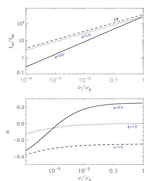
Figure 4: The upper panel shows the ratio of synchrotron flux from electrons in acceleration regions (PASs) and electrons in regions outside; three different lines correspond to three different values of $p$: 0.5 (solid line), 1.0 (dotted line) and 1.5 (dashed line). The parameters for these calculations are: $L=10^{48}$erg/s, $\Gamma=10$, $\sigma=10^{2}$, $R=10^{15}$cm, $\epsilon_{0}=0.1$, $\psi_{B}=0.1$, $\gamma^{\prime}_{p}=\gamma^{\prime}_{max}$, $\gamma^{\prime}_{min}=\gamma^{\prime}_{max}/10^{2}$, and $t^{\prime}_{cs}=10^{-3}\times R/(c\Gamma)$. The lower panel shows the spectral index for the observed flux, i.e. $\alpha=d\ln(f_{cs}+f_{dz})/d\ln\nu$ for the same three values of $p$. Note that for the parameters chosen for these calculations the observed flux is dominated by electrons radiating in PASs for $\nu\lower 2.0pt\hbox{$\,\buildrel\scriptstyle>\over{\scriptstyle\sim}\,$}10^{-3}\nu_{p}$ and therefore the spectral index in this frequency range is $\alpha\approx-(p-1)/2$, i.e. the spectrum is hard.

The observed spectrum is a superposition of synchrotron radiation from electrons in PASs and electrons outside acceleration regions. We have provided all the relevant equations to determine specific flux at an arbitrary frequency from these two sources. We note that if the observed flux between $\nu_{min}$ and $\nu_{p}$ is dominated by synchrotron radiation within PASs then the spectrum would be $f_{\nu}\propto\nu^{-(p-1)/2}$, which is harder by $\nu^{1/2}$ than the case where the flux comes mostly from electrons in the medium between PASs. Figure 4 shows the relative contributions of the two sources (upper panel), and the spectral index of the observed flux (lower panel), as a function of frequency. The figure clearly shows that the flux at $\nu_{p}$ is dominated by electrons in PASs and thus the spectral index is harder. Electrons outside PASs make the dominant contribution to the observed flux at sufficiently low frequencies (below $\nu_{p}/10^{2}$ for the parameters considered in Fig. 4), and therefore the spectrum is softer. This behavior — softening of spectrum with decreasing frequency — is opposite to what we observe in the synchrotron radiation from particles that are accelerated in shocks. This spectral feature may be a way to determine if magnetic or shock dissipation of jet energy is responsible for the observed radiation.

In practice, the spectral softening before the peak could be produced in a baryonic jet if there are multiple emission processes at work, for instance synchrotron radiation with a thermal component or synchrotron self-Compton (SSC). For a synchrotron + thermal component, the expected softening at low energies is very large which cannot be confused with the softening we expect for reconnection described above. It is more difficult to tell apart a kinetic jet with SSC radiation mechanism and a magnetic jet where synchrotron dominates. The SSC should produce two distinct peaks in the spectrum, one for synchrotron and one for inverse Compton, and in this case the radiation at lower energies dominated by the synchrotron process can be softer. The spectrum for the magnetic model on the other hand has just one peak, and therefore in principle it can be distinguished from the SSC model. However, in practice, the first peak for the SSC model may be at a frequency that is below the observing band, and that would make the task of identifying a Poynting jet more difficult. There are examples of low energy spectral softening in astrophysical objects, e.g., GRB 090926A (Ackermann et al. 2011), but it is difficult to say whether or not it is due to multiple components to the spectrum or from the spectral feature described in this paper. We looked for the spectral feature we predict for a magnetic reconnection model in solar flares where magnetic dissipation is widely believed be at work (e.g. Lin et. al, 2003). Unfortunately, solar flares have a large thermal component, so the presence of a soft spectral feature at low frequencies is difficult to discern in these transients.

The ratio of the luminosity in synchrotron and IC radiations is equal to the ratio of energy densities in magnetic field and photons. Since only a small fraction of energy in magnetic fields in dissipated in current sheets, it is expected that the IC luminosity of a Poynting jet would be smaller than the synchrotron luminosity. The IC spectrum, or to be precise synchrotron-self-Compton spectrum, is straightforward to calculate using the results for particle distribution and synchrotron spectrum described above.

2.4 Constraint on the number of current sheets in the jet

The radius interval where conversion of magnetic energy to thermal energy for a Poynting jet takes place depends on the magnetic field configuration and instabilities that develop in the jet. These are very difficult to calculate with any confidence. However, some general considerations described in this subsection provide broad guidance which can be used to constrain the dissipation radius and the number of current sheets in the jet.

Consider a short segment of the jet that was launched at radius $R_{0}$. The dissipation of magnetic energy in this segment could take place anywhere between $R_{0}$ and $\sim R_{d}$ (the deceleration radius of the jet), either gradually over this long distance interval or suddenly within a short distance. Once the reconnection gets started at one location in the jet, it could trigger magnetic field dissipation at other sites — possibly as a result of plasma outflow from this region or magnetic field reconfiguration propagating at Alfv́en speed and triggering reconnection at other sites — and these secondary reconnection sites lie in a region of the jet that is in causal contact with the current sheet triggering these events. It is unlikely that most of the energy of this segment of the jet under consideration will be dissipated at a radius smaller than $(\delta t)c\Gamma^{2}$ because of causality considerations (provided of course that different parts of this segment of the jet don’t independently develop instability and/or reconnection centers). We can describe the dissipation with radius as a monotonically increasing function of radius, $\zeta_{B}(R)$; $\zeta_{B}$ is the fraction of the magnetic energy in the segment that is dissipated or converted to bulk kinetic energy of the jet.

For reconnections in a jet consisting of stripped magnetic wind geometry (magnetic fields reversing direction over distance of $r_{0}$ in the lab frame), $\zeta_{B}\propto R^{1/3}$ (e.g. Drenkhahn and Spruit, 2002; Kumar & Zhang, 2014), and the process is completed at a radius $R_{c}\sim r_{0}\Gamma^{2}/\epsilon_{0}$; where $\epsilon_{0}$ as defined in §2.1 is the ratio of electric and magnetic fields and $v^{\prime}_{p}\sim\epsilon_{0}c$ is the speed for plasma flow into current sheets. So, although, the magnetic field dissipation process in this case is slow and extends over a large distance interval of $R_{0}$ — $r_{0}\Gamma^{2}/\epsilon_{0}\gg R_{0}$, roughly half of the magnetic energy is in fact dissipated within a factor of a few of $r_{0}\Gamma^{2}/\epsilon_{0}$. This follows from causality, i.e. the size of the region where magnetic field is dissipated cannot increase at a speed faster than light, and hence the radial width of region where field has been dissipated grows proportional to $R/\Gamma$ (in jet comoving frame) and that is the reason that a good fraction of magnetic energy dissipation occurs within a factor a few of the terminal radius where the dissipation process is completed. This property is likely to be generic, and independent of magnetic field geometry and reconnection model.

Current sheets are likely to form and disappear on a time short compared with the dynamical time ($R/(c\Gamma)$ in jet comoving frame). We envision that there are an average $\aleph_{s}$ PASs present in the region at any given time, for a time duration $\sim R/(c\Gamma)$, and the average length of these current sheets in jet comoving frame is $\ell^{\prime}_{s}$.

The total volume of plasma in the jet in the causally connected region at $R$ is

$${\cal V}^{\prime}_{c}\sim(R/\Gamma)^{3},$$ (53)

provided that the jet opening angle is $>\theta_{j}$. Since plasma flows into current sheets at speed $v^{\prime}_{p}\sim\epsilon_{0}c$, the total volume of plasma passing through current sheets in a dynamical time is

$${\cal V}^{\prime}_{plasma,cs}\sim\aleph_{s}{\ell^{\prime}_{s}}^{2}\epsilon_{0}(R/\Gamma).$$ (54)

If the fraction of the magnetic energy in the jet dissipated in this region is $\zeta_{B}(R)$, then that means that the total volume of plasma passing through current sheets in volume ${\cal V}^{\prime}_{c}$ should be $\zeta_{B}{\cal V}^{\prime}_{c}$. Thus, we obtain the number of PASs in the region to be

$$\aleph_{s}\sim[\zeta_{B}(R)/\epsilon_{0}]\left\{R/(\Gamma\ell^{\prime}_{s})\right\}^{2}.$$ (55)

A lower limit for $\aleph_{s}$ can be obtained by substituting $\ell^{\prime}_{s}\sim R/\Gamma$ in equation (55), which gives

$$\aleph_{s}\lower 2.0pt\hbox{$\,\buildrel\scriptstyle>\over{\scriptstyle\sim}\,$}\zeta_{B}(R)/\epsilon_{0}.$$ (56)

And a generous upper limit on the number of current sheets can be obtained by taking $\ell^{\prime}_{s}\sim\ell^{\prime}_{a}$ (the distance an electron travels in order to get accelerated to LF $\gamma^{\prime}_{max}$). Using (30) we find $\aleph_{s}\lower 2.0pt\hbox{$\,\buildrel\scriptstyle<\over{\scriptstyle\sim}\,$}5\times 10^{8}\zeta_{B}(R)\Gamma_{2}^{-5}R_{15}^{-1}L_{48}^{3/2}$. This upper limit is much too large to be of practical use. The length of an acceleration region can be much larger than $\ell^{\prime}_{a}$ when electron acceleration is balanced by radiative losses, and in that case far fewer number of PASs are needed to process magnetic energy to radiation. Let us take $\ell^{\prime}_{s}=\eta\ell^{\prime}_{a}$, with $\eta\sim 10^{3}$ that is needed to ensure that the observed radiation is dominated by electrons in PASs (as opposed to electrons in inter-PAS regions) and therefore the emergent spectrum is hard (see §2.3). This results in

$$\aleph_{s}\sim 5\times 10^{2}\zeta_{B}(R)\eta_{3}^{-2}\Gamma_{2}^{-5}R_{15}^{-1}L_{48}^{3/2}.$$ (57)

3 Discussion

This work was motivated in part by a puzzle regarding gamma-ray bursts. A broad class of models for $\gamma$-ray emission from GRBs is based on the jet being baryonic, which moves with a Lorentz factor $\lower 2.0pt\hbox{$\,\buildrel\scriptstyle>\over{\scriptstyle\sim}\,$}10^{2}$. The kinetic energy of baryons in the jet is converted to particle thermal energy via a series of shocks, and radiated away via the synchrotron process. According to this model, the spectrum below the peak should be $f_{\nu}\propto\nu^{-1/2}$ or softer whereas the observed spectra for most bursts are close to $\nu^{0}$, i.e. much harder than the baryonic jet model predicts (e.g. Ghisellini et al., 2000; Kumar & McMahon, 2008). The origin of this problem can be traced to the fact that particles are accelerated while crossing the shock front but otherwise they cool rapidly as they travel down-stream. Therefore, the number of electrons increases rapidly with decreasing LF ($dn^{\prime}_{e}/d\gamma^{\prime}_{e}\propto\gamma^{\prime-2}_{e}$ or faster) and that is the reason for the soft spectrum for a generic model that is based on dissipation of baryonic jet energy in shocks.

What we find is that if the GRB jet were not baryonic but Poynting, then the dissipation of magnetic fields and particle acceleration provides a way out this problem. This is because particles can be kept in acceleration regions for a time much longer than the their radiative cooling time, thereby preventing the development of a large population of lower energy electrons that give rise to a soft spectrum. The spectrum of radiation from electrons in the region in between PASs (where electrons are undergoing cooling without acceleration) is soft like that it is for the shock model, but the spectrum emanating from PASs is hard because the powerlaw index for the particle distribution function in current sheets has $p\approx 1$. We have shown in §2.3 that the observed spectrum, which is a superposition of contributions from the two regions (PASs and inter-PASs), is hard when the average time electrons spend in acceleration region is much larger than their synchrotron cooling time.

One of the general results reported here may be able to determine whether a jet is baryonic or Poynting — for a Poynting jet, the spectrum below the peak softens with decreasing frequency, which is opposite to the case of a baryonic jet where shocks convert jet energy to radiation via the synchrotron process.

4 Acknowledgments

PK would like to thank Fan Guo for useful discussions. We are grateful to Sera Markoff and an anonymous referee for offering numerous suggestions that significantly improved the paper.

References

• [1] Ackermann, M., Ajello, M., Asano, K., et al.Β 2011, ApJ, 729, 114
• [2] Begelman, M.Β C., Blandford, R.Β D., & Rees, M.Β J.Β 1984, Reviews of Modern Physics, 56, 255
• [3] Beloborodov, A. M., 2010, MNRAS 407, 1033
• [4] Beniamini, P. and Piran, T. 2014, MNRAS 445, 3892
• [5] Bessho, N., & Bhattacharjee, A.Β 2012, ApJ, 750, 129
• [6] Birn, J., Drake, J.Β F., Shay, M.Β A., et al.Β 2001, JGR, 106, 3715
• [7] Biskamp, D.Β 1986, Physics of Fluids, 29, 1520
• [8] Blandford, R.Β D., & Payne, D.Β G.Β 1982, MNRAS, 199, 883
• [9] Blandford, R.Β D., & Znajek, R.Β L.Β 1977, MNRAS, 179, 433
• [10] Cerutti, B., Uzdensky, D.Β A., & Begelman, M.Β C.Β 2012, ApJ, 746, 148
• [11] Coroniti, F.Β V.Β 1990, ApJ, 349, 538
• [12] Dermer, C. D., Chiang, J., Bottcher, M., 1999, ApJ 513, 656
• [13] Drake, J.Β F., Swisdak, M., Che, H., & Shay, M.Β A.Β 2006, Nat, 443, 553
• [14] Drenkhahn, G.Β 2002, AA 387, 714
• [15] Drenkhahn, G., Spruit, H. C., 2002, AA 391, 1141
• [16] Dungey, J.W. 1953, Phil. Mag. 44, 725
• [17] Giannios, D., & Spruit, H.Β C.Β 2006, AA, 450, 887
• [18] Ghisellini, G. & Celotti, A. 1999, AAS, 138, 527
• [19] Ghisellini, G., Celotti, A., Lazzati, D., 2000, MNRAS 313, L1
• [20] de Gouveia dal Pino, E.Β M., & Lazarian, A.Β 2005, AA, 441, 845
• [21] Guo, F., Li, H., Daughton, W. and Liu, Y-H, 2014, PRL 113, 155005
• [22] Hesse, M., & Zenitani, S., 2007, Physics of Plasmas, 14, 112102
• [23] Jaroschek, C.Β H., Treumann, R.Β A., Lesch, H., & Scholer, M.Β 2004, Physics of Plasmas, 11, 1151
• [24] Kennel, C. F., Coroniti, F. V. 1984, ApJ 283, 694
• [25] Komissarov, S. S., Barkov, M. V., Vlahakis, N., Konigl, A. 2007, MNRAS 380, 51
• [26] Kulsrud, R.Β M.Β 1998, Physics of Plasmas, 5, 1599
• [27] Kulsrud R.M. 2005, Plasma Physics for Astrophysics. Princeton, NJ: Princeton Univ. Press
• [28] Kumar, P., 1999, ApJ 523, L113
• [29] Kumar, P. Zhang, B., 2014, Physics Reports, http://dx.doi.org/10.1016/j.physrep.2014.09.008
• [30] Kumar, P., McMahon, E., 2008, MNRAS 384, 33
• [31] Larrabee, D. A., Lovelace, R. V. E., Romanova, M. M., 2003, ApJ 586, 72
• [32] Lin, R.Β P., Krucker, S., Hurford, G.Β J., et al.Β 2003, ApJ, 595, L69
• [33] Lovelace, R.Β V.Β E., Li, H., Koldoba, A.Β V., Ustyugova, G.Β V., & Romanova, M.Β M.Β 2002, ApJ, 572, 445
• [34] Lyubarsky, Y., & Kirk, J.Β G.Β 2001, ApJ, 547, 437
• [35] Meszaros, P. & Rees, M., 1993, ApJ 405, 278
• [36] MΓ©szΓ‘ros, P., & Rees, M.Β J.Β 1997, ApJ, 482, L29
• [37] Metzger, B.Β D., Giannios, D., Thompson, T.Β A., Bucciantini, N., & Quataert, E.Β 2011, MNRAS, 413, 2031
• [38] Michel, F.Β C.Β 1969, ApJ, 158, 727
• [39] Parker, E. N., 1957, JGR 62, 509
• [40] Petschek, H. E., 1964, The Physics of Solar Flares, Proceedings of the AAS-NASA Symposium Oct. 28-30 1963, Edited by Wilmot N. Hess. p.425
• [41] Rees, M. & Meszaros, P., 1994, ApJ 430, L93
• [42] Romanova, M.Β M., & Lovelace, R.Β V.Β E.Β 1992, AA, 262, 26
• [43] Rybicki, G. B., Lightman, A. P., 1979. Radiative processes in astrophysics, New York, Wiley-Interscience, 1979. 393 p.
• [44] Samtaney, R., Loureiro, N.Β F., Uzdensky, D.Β A., Schekochihin, A.Β A., & Cowley, S.Β C.Β 2009, Physical Review Letters, 103, 105004
• [45] Sironi, L., & Spitkovsky, A.Β 2011, ApJ, 741, 39
• [46] Sironi, L., & Spitkovsky, A.Β 2014, ApJ, 783, L21
• [47] Stern, B.E. & Poutanen, J., 2004, MNRAS 352, L35
• [48] Sweet, P.A., 1958, Proceedings of the IAU Symposiuomn on Electromagnetic Phenomena in Cosmical Physics, Stockholm, 1956
• [49] Syrovatskii, S.Β I.Β 1981, Annual review of astronomy and astrophysics, 19, 163
• [50] Tchekhovskoy, A., McKinney, J. C., Narayan, R., 2008, MNRAS 388, 551
• [51] Thompson, C. & Gill, R., 2014, ApJ 791, 46
• [52] Uzdensky, D.Β A., & Kulsrud, R.Β M.Β 2000, Physics of Plasmas, 7, 4018
• [53] Werner, G.Β R., Uzdensky, D.Β A., Cerutti, B., Nalewajko, K., & Begelman, M.Β C.Β 2014, arXiv:1409.8262
• [54] Yamada, M., Ji, H., Hsu, S., et al.Β 1997, Physical Review Letters, 78, 3117
• [55] Zenitani, S., & Hoshino, M.Β 2001, ApJ, 562, L63
• [56] Zweibel, E.G. and Yamada, M. 2009, Annu. Rev. Astro. Astrophys.47, 291
• [57]