Simple criteria for noise resistance of two qudit entanglement

Abstract

Too much noise kills entanglement. This is the main problem in its production and transmission. We use a handy approach to indicate noise resistance of entanglement of a bi-partite system described by $d\times d$ Hilbert space. Our analysis uses a geometric approach based on the fact that if a scalar product of a vector $\vec{s}$ with a vector $\vec{e}$ is less than the square of the norm of $\vec{e}$, then $\vec{s}\neq\vec{e}$. We use such concepts for correlation tensors of separable and entangled states. As a general form correlation tensors for pairs of qudits, for $d>2$, is very difficult to obtain, because one does not have a Bloch sphere for pure one qudit states, we use a simplified approach. The criterion reads: if the largest Schmidt eigenvalue of a correlation tensor is smaller than the square of its norm, then the state is entangled. this criterion is applied in the case of various types of noise admixtures to the initial (pure) state. These include white noise, colored noise, local depolarizing noise and amplitude damping noise. A broad set of numerical and analytical results is presented. As the other simple criterion for entanglement is violation of Bell’s inequalities, we also find critical noise parameters to violate specific family of Bell inequalities (CGLMP), for maximally entangled states. We give analytical forms of our results for $d$ approaching infinity.

I Introduction

Detection of entanglement is a fundamental problem in quantum information . Many theoretical works have been done to establish a criterion to identify multipartite entanglement Horodecki09 ; Guhne09 ; Vicente ; Laskowski11 ; Laskowski15 ; Huber2010 ; Spengler . Although not all of these works have direct impact on experiments, still they provide a mathematical background to understand the phenomena.

An arbitrary density operator for two qudits can be written as

$$\rho = \frac{d-1}{2d}\Big{(}M_{0}\otimes M_{0}+\sum_{i,j=1}^{d^{2}-1}T_{ij}M_{i}\otimes M_{j}$$

$$+ (d-1)\sum_{i=1}^{d^{2}-1}(T_{0i}M_{0}\otimes M_{i}+T_{i0}M_{i}\otimes M_{0})\Big{)},$$

where $T_{ij},T_{0i},T_{i0}$ are components of the correlation tensor $\hat{T},$ and $M_{i}(\text{except}~{}i=0)$ are the generalized Gell-Mann matrices (see Appendix A for details) with $M_{0}=\sqrt{\frac{2}{d(d-1)}}\openone_{d}.$ The components $T_{ij}$ are real and given by $T_{ij}=c(d)\textrm{Tr}[\rho(M_{i}\otimes M_{j})]$, where the coefficient $c(d)$ depends on the dimensionality (see Appendix B).

In  Badziag08 it has been shown that the correlation tensor could be utilized to construct entanglement indicators. The nonlinear character of the resulting entanglement indicator of Badziag08 make them more versatile than linear entanglement witnesses. The study of  Badziag08 was mainly done for multi-qubit systems. Here, we use the geometric approach of  Badziag08 to detect entanglement for pairs of systems, more complicated than qubits. In our approach we do not study the dynamics of noise, but we concentrate on properties of the state after evolving through a noisy channel. The white noise usually arises due to imperfections in experimental set up, while a “colored” noise can appear when multi particle entanglement is produced via multiple emissions  SEN . We also analyze the effects of different local noises, modeling random environment and dissipative process Nielsen_book .

We find that in some of the cases there exist significant differences in numerical values of the critical noise admixture parameters for having entanglement after a transfer via various noisy channels. A study of this kind was done for qubits in Ref. Laskowski10 . Here, we study higher dimensions. Note that, a different approach to obtain the criterion of separability of entangled qutrits in noisy channel is given in Ref. Chcińska .

Another way to detect entanglement is to violate Bell inequalities Bell64 . In our paper, we discuss resistance to noise of Bell-type inequalities for arbitrary dimension $d,$ e.g. Collins-Gisin-Linden-Massar-Popescu (CGLMP) inequality CGLMP .

II Simplified entanglement condition

Separable states can be described by a fully separable extended correlation tensor, $\hat{T}^{\text{sep}}=\sum_{i}p_{i}\hat{T}_{i}^{\text{prod}}$, where $\hat{T}_{i}^{\text{prod}}=\hat{T}_{i}^{1}\otimes\hat{T}_{i}^{2}$, and each $\hat{T}_{i}^{k}$ is the $d^{2}$-dimensional generalized Bloch vector of $k$th single qudit subsystem. To produce entanglement conditions we employ a geometrical approach based on correlation functions, which was introduced in Ref. Badziag08 . The criterion has the following form: the state $\rho$ described by its correlation tensor $\hat{T}$ is entangled, if

$$\max_{\hat{T}^{\text{prod}}}(\hat{T},\hat{T}^{\text{prod}})<(\hat{T},\hat{T})=||\hat{T}||^{2}.$$ (2)

The scalar product may be defined in various ways, provided it satisfies all required axioms. However the simplest choice is :

$$(\hat{X},\hat{Y})=\sum_{i,j=1}^{d^{2}-1}X_{ij}Y_{ij}.$$ (3)

In such a case, the maximum of the left-hand side of Eq. (2) can be obtained by the highest generalized Schmidt coefficient of the correlation tensor $\hat{T}$ as

$$T_{\text{max}}=\max_{\vec{m}_{1},\vec{m}_{2}}(\hat{T},\vec{m}_{1}\otimes\vec{m}_{2}),$$ (4)

where $\vec{m}_{k}$ is a $(d^{2}-1)$-dimensional generalized Bloch vector which describes a quantum state of $k$th subsystem. Note that, for $d>2$ we do not have a Bloch sphere. Thus $\vec{m}_{k}$’s represent the admissible Bloch vectors which represent a physical state. One can also take the maximum of the left-hand side of (2) as the square root of the highest eigenvalue of $TT^{\dagger}$, denoted by $L_{\text{max}}$. However, note that $L_{\text{max}}\geq T_{\text{max}},$ and this estimate gives a less robust criterion for entanglement. Still it is technically much easier, and thus we shall use it.

III Basic aims

We analyze entanglement of bipartite quantum states which are initially pure. For technical reasons we always put them in the Schmidt form:

$$|\psi\rangle=\sum_{i=0}^{d-1}c_{i}|ii\rangle.$$ (5)

We study various noisy channels, i.e., white, product, colored, local depolarizing and amplitude damping. In some cases, one can define a critical parameter $v_{\text{crit}}$ for the noisy output, of the form $\rho(v)=v|\psi\rangle\langle\psi|+(1-v)\rho_{\text{noise}}$, such that for $v>v^{d}_{\text{crit},ENT}$ the state $\rho(v)$ is entangled. The action of a channel on a density matrix of a two-qudit can also be written in terms of its operation elements, more precisely $\rho\to\sum_{u,v}E_{u}(p)\otimes E_{v}(p)\rho(E_{u}(p)\otimes E_{v}(p))^{\dagger}$, where $E_{l}$ is an operation element of the channel parametrized by $p,$ a certain strength parameter to be specified later. We define this parametrization in such a way, so that $p=1$ defines no noise, just unitary(local) evolution, while $p=0$ signifies the maximally noisy state leaving the channel. Hence, one can show presence of entanglement by satisfying the condition $p>p^{d}_{\text{crit},ENT}.$ Thus such a description is a generalization of the one involving $v_{\text{crit}}.$ We introduce a quantity

$$\xi(p^{d}_{\text{crit},ENT})=\text{min}\left(\left(\frac{||\hat{T}(p^{d}_{\text{crit},ENT})||^{2}}{||\hat{T}(p=1)||^{2}}\right)^{\frac{1}{2}},1\right)$$ (6)

to compare different noisy channels on the same footing. In order to check the entanglement condition (2), we put the correlation tensor of a state $\eqref{state0}$ in a Schmidt form itself. The general form of the tensor elements is given in Appendix C. Note that the Schmidt form of the state (5) does not imply a diagonal form of the corresponding tensor. Even for a two-qutrit state non-diagonal elements appear. This is not the case for qubits. Because of, the above reason, calculations of $L_{\text{max}}$ require the diagonalization of the tensor, which is a computationally difficult problem even for small $d$.

For white, product, and colored noises we analytically compute the critical parameter $v^{d}_{\text{crit},ENT}$ for the maximally entangled states (diagonal form of the correlation tensor)of a pair of qudits:

$$|\psi_{\text{max}}^{d}\rangle=\frac{1}{\sqrt{d}}\sum_{i=0}^{d-1}|ii\rangle$$ (7)

We present results for arbitrary $d$ and for $d\to\infty$.

We also analyze all non-maximally entangled pure initial states of qutrits ($d=3$), parametrized as follows:

$$|\psi^{3}(\alpha,\beta)\rangle = \cos\alpha|00\rangle+\sin\alpha\sin\beta|11\rangle$$ (8)

$$+ \sin\alpha\cos\beta|22\rangle.$$

The study is also done for lower Schmidt rank states, for $d=3,4$:

$$|\psi^{d}_{\textrm{rank-}k}\rangle=\sum_{j=d-k}^{d-1}c_{j}|jj\rangle,$$ (9)

where $k<d$ and $\sum_{j=d-k}^{d-1}|c_{j}|^{2}=1.$

IV Results for various types of noise

IV.1 White noise

White noise is represented by an admixture of the totally mixed state. A mixture of white noise and two-qudit pure state $|\psi\rangle$ can be written as

$$\rho_{\text{white}}(v)=v|\psi\rangle\langle\psi|+\frac{1-v}{d^{2}}\openone_{d}\otimes\openone_{d}.$$ (10)

Since white noise has no correlations, the correlation tensor $\hat{T}(v)$ for the state $\rho_{\text{white}}(v)$ is given by $\hat{T}(v)=v\hat{T}$. In the case of the maximally entangled state, only diagonal components of the tensor are nonzero and given by $T_{ii}(v)=\pm v/(d-1)$ for $i\in\{1,2,\dots,d^{2}-1\}$. Therefore, we have $L_{\text{max}}=v/(d-1)$ and $||\hat{T}(v)||^{2}=v^{2}(d+1)/(d-1)$. Using the criterion (2), we can conclude that the state (10) is entangled if $v>(d+1)^{-1}$. This recovers the result of Ref. Werner89 . In the limit of $d\to\infty$, the critical value $v^{d}_{\text{crit},ENT}$ tends to 0.

For the case of two-qutrit non-maximally entangled states (8)we obtain $L_{\text{max}}=v(8+\sqrt{K})/16$ and $||\hat{T}(v)||^{2}=v^{2}(2-K/64)$, where $K=31+12\cos 2\alpha+21\cos 4\alpha+24\cos 4\beta\sin^{4}\alpha$. In Fig. 1, we present the critical values $v^{3}_{\text{crit},ENT}$. The pure state (8) is entangled for all $\alpha$ and $\beta$ except for $\alpha=0$, $\{\alpha=\pi/2,\beta=0\}$, and $\{\alpha=\pi/2,\beta=\pi/2\}$. The lowest value of $v^{3}_{\text{crit},ENT}=0.25$ is obtained by the maximally entangled state $|\psi_{\text{max}}^{3}\rangle$.

In Table 2 we present the numerical results for states $\eqref{eq:SR_state}.$ They are for two-qutrit states of the Schmidt form $\frac{1}{\sqrt{2}}(|11\rangle+|22\rangle),$ and of two-ququart states $\frac{1}{\sqrt{2}}(|22\rangle+|33\rangle)$ and $\frac{1}{\sqrt{3}}(|11\rangle+|22\rangle+|33\rangle).$ All this is compared with proper maximally entangled states. The analysis shows that the lower is the Schmidt rank of such states the more fragile is their entanglement.

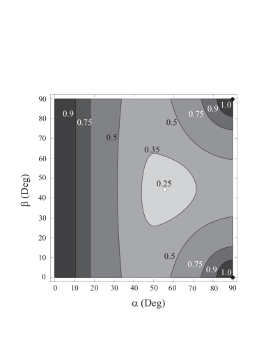
Figure 1: The critical values $v_{\text{crit}}$ to detect entanglement for two-qutrit non-maximally entangled states (8) and white noise admixture. For $v>v^{3}_{\text{crit},ENT}$, the state is entangled. The lowest critical value, $v^{3}_{\text{crit},ENT}=0.25$, is obtained for the maximally entangled state $|\psi^{3}_{\text{max}}\rangle$.

IV.1.1 White noise treated as local depolarizing noise

A $d$-dimensional quantum state exiting a local depolarizing channel is given by

$$\Lambda_{r}^{\text{depol}}(\rho)=(1-r)\rho+\frac{r}{d}\openone.$$ (11)

The use of such a formalism gives us a method of estimating how much noise (disturbance) is introduced per qudit. With probability $1-r$ the initial state $\rho$ still remain unaltered by the decoherence. To describe the local depolarizing effect on a two-qudit system, one can use the following transformation of the generalized Gell-Mann matrices:

$$\Lambda_{r}^{\text{depol}}(M_{k})=(1-r)M_{k},$$ (12)

where $k\in\{1,2,\dots,d^{2}-1\},$ and make the replacement in $T_{ij}=c(d)\textrm{Tr}[\rho(M_{i}\otimes M_{j})].$

For the maximally entangled state (7), after such a transformation only diagonal components of the correlation tensor are nonvanishing, and they read

$$T_{ii}(r)=\pm\frac{(1-r)^{2}}{(d-1)}~{}~{}~{}\text{for}~{}i\in\{1,2,\dots,d^{2}-1\}.$$ (13)

Therefore, we have $L_{\text{max}}=(1-r)^{2}/(d-1)$ and $||\hat{T}(r)||^{2}=(1-r)^{4}(d+1)/(d-1)$. We define $1-r=p$, the critical value $p^{d}_{\text{crit},ENT}$ in local depolarized channel is obtained as

$$p^{d}_{\text{crit},ENT}=(d+1)^{-\frac{1}{2}}.$$ (14)

We see that when $d\to\infty$, $p^{d}_{\text{crit},ENT}\to 0$. Thus with increasing d the maximal entanglement is more and more resistant with respect to the depolarizing noise.

Our study for arbitrary (initially) pure states of two qutrits (8) gives $L_{\text{max}}=p^{2}(8+\sqrt{K})/16$ and $||\hat{T}(p)||^{2}=p^{4}(2-K/64)$. The critical values $p^{d}_{\text{crit},ENT}$ are ploted in Fig. 2. It is entangled for all $\alpha$ and $\beta$ except those related to product states: $\alpha=0$, $\{\alpha=\frac{\pi}{2},\beta=0\}$ and $\{\alpha=\frac{\pi}{2},\beta=\frac{\pi}{2}\}$. The lowest value of $p^{3}_{\text{crit},ENT}=0.5$ is obtained by the maximally entangled state (7). In Tab. 1 we give numerical results of the critical values $p^{d}_{\text{crit},ENT}$ for lower Schmidt rank states $\eqref{eq:SR_state}$ for $d=3,4.$ We see that for a specific dimension, entangled states of lower Schmidt rank are less resistant to local depolarizing noise than entangled states of higher Schmidt rank. Thus the new analysis does not change the picture much.

For local depolarizing channel $||\hat{T}(p^{d}_{\text{crit},ENT})||^{2}=\frac{1}{d^{2}-1}$ and $||\hat{T}(p=1)||^{2}=\frac{d+1}{d-1}$ for the maximally entangled state which yields $\xi(p^{d}_{\text{crit},ENT})=\frac{1}{d+1}.$ This is identical to $v^{d}_{\text{crit},ENT}$ to detect entanglement for the maximally entangled state in a global depolarizing noisy channel (white noise).

Figure 2: Critical values $p^{3}_{\text{crit},ENT}$ for entanglement detection are shown for two-qutrit non-maximally entangled state under local depolarizing noise. The lowest critical value, $p^{3}_{\text{crit},ENT}=0.5$, is achieved for the maximally entangled state $|\psi^{3}_{\text{max}}\rangle$.

IV.2 Product noise

We consider the following output states:

$$\rho_{\text{prod}}(v)=v|\psi\rangle\langle\psi|+(1-v)\rho_{a}\otimes\rho_{b},$$ (15)

where $\rho_{i}=\sum_{j=0}^{d-1}|c_{j}|^{2}|j\rangle_{i}\langle j|$ is the reduced density matrix of the $i$th subsystem. The critical values $v^{3}_{\text{crit},ENT}$ are presented in Fig. 3. The lowest critical value $v^{3}_{\text{crit},ENT}=0.25$ is also obtained by the maximally entangled state $|\psi^{3}_{\text{max}}\rangle$ (for this state the product noise is reduced to white noise) Note that $v^{3}_{\text{crit},ENT}=1$ for product states, whereas in the limits $\alpha\to 0$, $\{\alpha\to\pi/2,\beta\to 0\}$, or $\{\alpha\to\pi/2,\beta\to\pi/2\}$, the state (15) is entangled for the critical visibility approaching 0.6039. In other words, our geometrical method is very sensitive in the presence of product noise.

Figure 3: The critical values $v^{3}_{\text{crit},ENT}$ to indicate entanglement for product noise. For $\alpha\to 0$, $\{\alpha\to\pi/2,\beta\to 0\}$, and $\{\alpha\to\pi/2,\beta\to\pi/2\}$, the state $\eqref{prod}$ is entangled for the critical visibility approaching $0.6039$.

IV.3 Colored product noise

In the special case of output states

$$\rho_{\text{c}}(v)=v|\psi_{\text{max}}^{d}\rangle\langle\psi_{\text{max}}^{d}|+(1-v)\hat{\pi}_{c}\otimes\hat{\pi}_{c},$$ (16)

with $\hat{\pi}_{c}=|d-1\rangle\langle d-1|,$ the correlation tensor of the state (16) has the following non-vanishing components:

$$T_{ii}(v)=\left\{\begin{array}[]{ll}\pm\,\frac{v}{d-1}&\text{for}\,\,\,i\in\{1,\dots,d^{2}-2\},\\ 1-\frac{v(d-2)}{d-1}&\text{for}\,\,\,i=d^{2}-1.\end{array}\right.$$ (17)

In order to get more efficient entanglement condition, we consider a generalized version of the criterion of Eq. (2)

$$\max_{\hat{T}^{\text{prod}}}(\hat{T},\hat{T}^{\text{prod}})_{G}<||\hat{T}||_{G}^{2},$$ (18)

where now the scalar product is defined by a positive semidefinite diagonal metric $G$ Badziag08 :

$$(\hat{X},\hat{Y})_{G}=\sum_{i,j=1}^{d^{2}-1}X_{ij}G_{ij}Y_{ij}.$$ (19)

We consider a diagonal metric $G$ with the following nonzero elements: $G_{ii}=1$ for $i\in\{1,2,\dots,d^{2}-2\}$ and $G_{d^{2}-1d^{2}-1}=v$. With such a metric, the left-hand side (18) reads $L_{\text{max}}^{G}=v[1-v(d-2)/(d-1)]$ and $||\hat{T}(v)||_{G}^{2}$ as $v[1+v(-6+6d-d^{2}+v(d-2)^{2})/(d-1)^{2}]$. For $d\geq 2$, $||\hat{T}(v)||_{G}^{2}$ is always greater than $L_{\text{max}}^{G}$. It implies that the state $\rho_{\text{c}}(v)$ is always entangled except $v=0$, i.e., even for an infinitesimally small $v$ the state is entangled.

IV.4 Amplitude damping noise

An amplitude damping channel can be described by a process of energy dissipation of a quantum system to environment. The transition of excitation occurs between excited state and the ground state with a finite probability. No transition is allowed between excited states. Such an amplitude damping channel can be described by:

$$\rho_{\text{AD}}(r)=\!\!\!\!\sum_{k,m=0}^{d-1}{E_{k}(r)\otimes E_{m}(r)\rho(E_{k}(r)\otimes E_{m}(r))^{\dagger}},$$ (20)

where

$$E_{0} = |0\rangle\langle 0|+\sqrt{1-r}\sum_{i=1}^{d-1}|i\rangle\langle i|,$$

$$E_{j} = \sqrt{r}~{}|0\rangle\langle j|,~{}~{}~{}j\in\{1,2,\dots,d-1\}.$$ (21)

The transformation of the generalized Gell-Mann matrices is given by

$$M_{j}(r)=\left\{\begin{array}[]{ll}\sqrt{1-r}M_{j}{}{}&\text{for}~{}M_{j}\in\{M_{1,k}^{s(\text{or}\,a)}\}\\ (1-r)M_{j}{}&\text{otherwise},\end{array}\right.$$ (24)

where $j\in\{1,2,\dots,d^{2}-d\},k\in\{2,3,\dots,d\}$, the $M_{1,k}^{s(\text{or}\,a)}$ is the symmetric (or antisymmetric) Gell-Mann matrices (see Appendix A for details). Here, we do not consider the transformation rule for diagonal Gell-Mann matrices as they are redundant in later calculation.

For the two-qudit maximally entangled state (7), we have the following nonzero components of the correlation tensor

$$T_{ii}(r)=\begin{cases}\pm\frac{(1-r)}{(d-1)}~{}~{}&\text{for}~{}M_{i}\in\{M_{1,k}^{s(\text{or}\,a)}\}\\ \pm\frac{(1-r)^{2}}{(d-1)}~{}~{}&\text{otherwise},\end{cases}$$ (25)

where $i\in\{1,2,\dots,d^{2}-d\}$. Although $T_{ij}(r)$ are non zero for $i,j\in\{d^{2}-d,d^{2}-d+1,...d^{2}-1\},$ still they do not have any impact in our calculation to obtain the sufficient condition for entanglement. More precisely, to calculate the critical value $p_{\text{crit}}$ for amplitude damping noise with a specific combination of components of correlation tensor, we use the generalized criterion (18) involving the diagonal metric; $G_{ii}=1$ for $i\in\{1,2,\dots,d^{2}-d\}$ and other components are zero. As a result, we have $L_{\text{max}}=(1-r)/(d-1)$ and $||\hat{T}(r)||^{2}=(1-r)^{2}\left[2+(d-2)(1-r)^{2}\right]/(d-1)$. Thus, the entanglement criterion (18) reduces to $(d-2)p^{3}+2p>1$, where $p=1-r$. We find that for $d>2$ the state is entangled if the value $p$ exceeds the critical value

$$p^{d}_{\text{crit},ENT}=\left(\frac{1}{2(d-2)}\right)^{1/3}\left(1-\frac{A^{1/3}}{B^{2}}\right)B,$$ (26)

where $A=2^{5}/[3^{3}(d-2)]$ and $B=[1+(1+A)^{1/2}]^{1/3}$. The critical value $p^{d}_{\text{crit},ENT}$ goes to zero when $d\to\infty$.

It is worth noting that non-maximally entangled states for $d=3,4$ in Eq. (8) are more robust than the maximally entangled state (7) against this type of noise. The corresponding non-maximally entangled states are $|\psi(\frac{4\pi}{15},\frac{\pi}{4})\rangle$ for $d=3$ and $|\psi^{4}_{\text{nmax}}\rangle=\cos(0.853)|00\rangle+\frac{1}{\sqrt{3}}\sin(0.853)(|11\rangle+|22\rangle+|33\rangle).$ The critical values $p^{3}_{\text{crit},ENT}$ are ploted in Fig. 4. In Table 1 we show numerical results of the critical values $p^{d}_{\text{crit},ENT}$ for lower Schmidt rank states $\eqref{eq:SR_state}$ for $d=3,4.$ It is found that the maximally entangled states  $\eqref{eq:MES}$ of lower Schmidt rank are less robust than the maximally entangled states of higher Schmidt rank. As a matter of fact the positive semidefinite diagonal metric $G$ is not unique, one can obtain lower values for $p^{d}_{\text{crit},ENT}$ than the results presented in our manuscript with the optimal $G.$

Also, we check critical parameter in $\eqref{square}$ for the maximally entangled state $\eqref{eq:MES}.$ Here $||\hat{T}(p^{d}_{\text{crit},ENT})||^{2}=\frac{(p^{d}_{\text{crit},ENT})^{2}}{d-1}(2+(d-2)(p^{d}_{\text{crit},ENT})^{2})$ and $||\hat{T}(p=1)||^{2}=\frac{d}{d-1}$ which yields $\xi(p^{d}_{\text{crit},ENT})=p^{d}_{\text{crit},ENT}(2+(d-2)(p^{d}_{\text{crit},ENT})^{2})^{\frac{1}{2}}d^{-\frac{1}{2}}.$ Hence, $\xi(p^{d}_{\text{crit},ENT})\to 0$, when $d\to\infty.$ Due to our entanglement criterion we obtain lower value for $\xi(p^{3}_{\text{crit},ENT})$ for a specific non-maximally entangled state Eq. (8) than the maximally entangled state (7) while analyzing for amplitude damping noise. The corresponding non-maximally entangled state is $|\psi(\frac{7\pi}{18},\frac{\pi}{4})\rangle$ for $d=3.$ For this specific state $|\psi(\frac{7\pi}{18},\frac{\pi}{4})\rangle,$ we obtain $p^{3}_{\text{crit},ENT}=0.4990.$ The critical values $\xi(p^{3}_{\text{crit},ENT})$ are plotted in Fig. 5. A comparison between values of $v^{d}_{\text{crit},ENT}$ and $\xi(p^{d}_{\text{crit},ENT})$ parameter, calculated for white or local depolarizing noise and amplitude damping noise, respectively is shown in Table 2 .

Figure 4: We show the critical value $p^{3}_{\text{crit},ENT}$ of entanglement identification for non-maximally entangled state of qutrits for amplitude damping noise. The lowest value( 0.447(approximate)) for $p^{3}_{\text{crit},ENT}$ is obtained for the state $|\psi(\frac{4\pi}{15},\frac{\pi}{4})\rangle$(8)

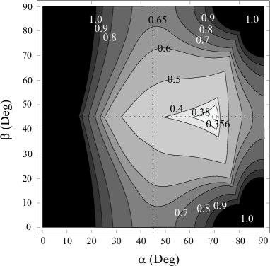
Figure 5: We show the critical value $\xi(p^{3}_{\text{crit},ENT})$ of entanglement identification for non-maximally entangled state of qutrits for amplitude damping noise. The lowest value (0.3560) for $p^{3}_{\text{crit},ENT}$ is obtained for the state $|\psi(\frac{7\pi}{18},\frac{\pi}{4})\rangle$(8)

noise	$d$	$|\psi_{\text{max}}^{d}\rangle$	$|\psi^{d}_{\text{rank-}2}\rangle$	$|\psi^{d}_{\textrm{rank-}3}\rangle$	$|\psi^{d}_{\text{nmax}}\rangle$
	2	0.5773	-	-	-
local depolarizing	3	0.5	0.6546	-	-
	4	0.4472	0.6794	0.5283	-
	2	0.5	-	-	-
amplitude damping	3	0.4534	0.8165	-	0.4465
	4	0.4239	0.8660	0.6124	0.4074

Table 1: Summary of the critical values $p^{d}_{\text{crit},ENT}$ to detect entanglement for the various bipartite states under depolarizing and amplitude damping noises: the maximally entangled state $|\psi_{\text{max}}^{d}\rangle$, the non-maximally entangled state $|\psi^{d}_{\text{nmax}}\rangle$, and the lower Schmidt rank states $|\psi^{d}_{\text{rank-}k}\rangle$. For amplitude damping noise, the specific non-maximally entangled states present lower critical value $p^{d}_{\text{crit},ENT}$ than the maximally entangled ones. The specific states are presented below Eq. (26).

noise	$d$	$|\psi_{\text{max}}^{d}\rangle$	$|\psi^{d}_{\text{rank-}2}\rangle$	$|\psi^{d}_{\textrm{rank-}3}\rangle$	$|\psi^{d}_{\text{nmax}}\rangle$
	2	0.3333	-	-	-
local depolarizing	3	0.25	0.4285	-	-
	4	0.2	0.4615	0.2790
	2	0.5	-	-	-
amplitude damping	3	0.3888	0.6667	-	0.3560
	4	0.3256	0.750	0.3750	-

Table 2: A summary of the critical values $\xi(p^{d}_{\text{crit},ENT})$ for local depolarizing noises, and amplitude damping noise in detection of entanglement for $|\psi_{\text{max}}^{d}\rangle$ and the lower Schmidt rank states $|\psi^{d}_{\text{rank-}k}\rangle$ is given in a tabular form. As a mater of fact, $\xi(p^{d}_{\text{crit},ENT})$ computed for each cases with local depolarizing noise is identical to $v^{d}_{\text{crit},ENT}$ obtained for the identical states with white noise. Also, for amplitude damping noise, the specific non-maximally entangled state presents lower critical values $\xi(p^{3}_{\text{crit},ENT})$ than the maximally entangled one. The specific state is $|\psi(\frac{7\pi}{18},\frac{\pi}{4})\rangle$ for $d=3.$

V Testing Entanglement with Bell inequalities

In this section, we analyze noise resistance of violation of Bell-type inequalities for the bipartite quantum states (5). To this end, we employ the CGLMP inequality introduced in Ref. CGLMP , which can be written as

$$I_{d}=\sum_{k=0}^{\lfloor\frac{d}{2}\rfloor-1}\left(1-\frac{2k}{d-1}\right)\left(\mathcal{B}_{k}-\mathcal{B}_{-(k+1)}\right)\leq 2,$$ (27)

where $\mathcal{B}_{k}=P(A_{1}=B_{1}+k)+P(B_{1}=A_{2}+k+1)+P(A_{2}=B_{2}+k)+P(B_{2}=A_{1}+k)$.

We compare robustness of violation of the CGLMP inequality, with respect to white noise, in case of the maximally entangled state $|\psi^{d}_{\text{max}}\rangle$ (7), presented in CGLMP with robustness of violation by the same state under different noisy channels.

V.1 White noise

In this section we give an analytical solution for the critical visibility to violate the inequality 27 with the maximally entangled states and then consider the case for $d\to\infty.$

Since white noise does not contribute to the violation of the CGLMP inequality (27) as stated in Ref. (27), the quantum value for the state $\rho_{\text{white}}(v)$ in Eq. (10) is given by

$$I^{d}_{QM}[\rho_{\text{white}}(v)]=vI^{d}_{QM}[|\psi\rangle].$$ (28)

Therefore the critical parameters for the violation of the CGLMP inequality (27) are given by

$$v_{crit,LR}^{d}=2/I^{d}_{QM}[|\psi\rangle].$$ (29)

and equal: $v_{crit,LR}^{2}\approx 0.7073$, $v_{crit,LR}^{3}\approx 0.6962$, $v_{crit,LR}^{4}\approx 0.6906$ and $v_{crit,LR}^{\infty}\approx 0.6734$ CGLMP . Note that the lowest critical visibility for the CGLMP inequality is achieved by non-maximally entangled states ACIN and studied in details (for $d=3$) in Ref. GRUCA2 . The lowest critical visibility ($v^{3}_{\text{crit},LR}$=0.6861)(Ref. GRUCA2 ) to violate CGLMP inequality in $d=3$ is obtained for non-maximally entangled state $|\psi^{3}(1.0601,0.7854)\rangle$ (see  $\eqref{eq:NMES}).$ For this specific non-maximally entangled state $|\psi^{3}(1.0601,0.7854)\rangle,$ we obtain $v^{3}_{\text{crit},ENT}=0.2883.$

V.1.1 White noise treated as local depolarizing channel

In this section we check the robustness of CGLMP inequality in a local depolarizing channel with maximally entangled state $|\psi^{d}_{\text{max}}\rangle$.

Following the transformation rules for the Gell-Mann matrices shown in 12, the state $|\psi^{d}_{\text{max}}\rangle$ after local depolarizing channel can be written as

$$\rho_{\text{depol}}(r)=(1-r)^{2}|\psi^{d}_{\text{max}}\rangle\langle\psi^{d}_{\text{max}}|+\frac{r(2-r)}{d^{2}}\openone_{d}\otimes\openone_{d}.$$ (30)

Since the noise part does not contribute to the Bell expression (27) with quantum mechanical observables, leads to the following condition for the critical parameters for the violation of (27):

$$p_{crit,LR}^{d}=\sqrt{2/I^{d}_{QM}[|\psi\rangle]},$$ (31)

where $p^{d}_{crit,LR}=(1-r^{d}_{crit,LR}).$ The results are given in Tab. 3. However in terms of visibility $v^{d}_{crit,LR}$, the result is identical with $\eqref{wnn}.$

$d$	depolarizing noise	amplitude damping noise
2	0.8410	0.7071
3	0.8344	0.7468
4	0.8310	0.7647
5	0.8290	0.7750
10	0.8248	0.7954
$\infty$	0.8206	0.8206

Table 3: The critical parameter to indicate violation of CGLMP inequality, $p^{d}_{crit,LR}$ are calculated for local depolarizing noise and amplitude damping noise for the bipartite maximally entangled state in higher dimensional systems.

V.2 Colored noise

In this section we check the violation of CGLMP inequality by the maximally entangled state , $|\psi^{d}_{\text{max}}\rangle$ III mixed with colored noise 16. Numerically we find that for $d=3$ instead of choosing settings $(\ref{settings})$ if we choose generalized $SU(3)$ transformation matrix, then $\eqref{Bell}$ is violated whenever $v>0.$

V.3 Amplitude damping channel

The same as in the previous cases, we examine the violation of the CGLMP inequality with state $|\psi^{d}_{\text{max}}\rangle$.

The state $|\psi^{d}_{\text{max}}\rangle$ after amplitude damping channel (IV.4) is given by

$$\rho_{\text{AD}}(r)=$$ (32)

$$\frac{1+r^{2}(d-1)}{d}|00\rangle\langle 00|+\frac{(1-r)^{2}}{d}\sum_{m,k\neq 0}^{d-1}|mm\rangle\langle kk|$$

$$+ \frac{(1-r)}{d}\left[\sum_{m\neq 0}^{d-1}|mm\rangle\langle 00|+\sum_{k\neq 0}^{d-1}|00\rangle\langle kk|\right]$$

$$+ \frac{r(1-r)}{d}\left[\sum_{m\neq 0}^{d-1}|m0\rangle\langle m0|+\sum_{k\neq 0}^{d-1}|0k\rangle\langle 0k|\right].$$

We numerically check the critical parameters for $d=2,3,4,5,10$. The results are given in Table 3.

We see that the critical parameter increases with the dimension. It has a tendency to attain saturation for very large $d$. We give an analytical result for $d$ tends to $\infty$ in Appendix (D). However, the lowest critical visibility ($p^{3}_{\text{crit},LR}$=0.7316) to violate CGLMP inequality in $d=3$ is obtained for non-maximally entangled state $|\psi^{3}(0.8730,0.6449)\rangle$ (see  $\eqref{eq:NMES}).$ For this specific non-maximally entangled state we obtain $p^{3}_{\text{crit},ENT}=0.5,$ whereas $\xi(p^{3}_{\text{crit},ENT})=0.4513.$ Also we check $p^{3}_{\text{crit},LR}$ for the specific non-maximally entangled state $|\psi^{3}(\frac{4\pi}{15},\frac{\pi}{4})\rangle,$ which gives the lowest $p^{3}_{\text{crit},ENT}.$ We obtain $p^{3}_{\text{crit},LR}=0.7429$ for the state. We extend our calculation by checking $p^{3}_{\text{crit},LR}$ for the non-maximally state $|\psi^{3}(\frac{7\pi}{18},\frac{\pi}{4})\rangle$ for which we obtain the lowest $\xi(p^{3}_{\text{crit},ENT})$ considering all two-qutrit states. The value is obtained as $0.8640.$

Although for $d\to\infty$, $p^{\infty}_{\text{crit},LR}$ to violate $\eqref{Bell}$ in presence of local depolarizing noise coincides (see Tab. 3) with the same parameter obtained in case of amplitude damping noise but in lower dimensions the variation in $p^{d}_{\text{crit},LR}$ in case of amplitude damping noise differs with the one for local depolarizing noise.

V.4 Fidelity of quantum states with critical noise

In this section we give analytic expression of fidelity, i.e., the measure of closeness between two quantum states, e.g., the state after noisy channel with the pure state (here we only consider the maximally entangled state $\eqref{eq:MES})$ of the system under investigation.

Usually fidelity $F$ for two quantum states is defined as $\sqrt{\langle\phi|\rho|\phi\rangle},$ where $\phi$ is a pure state whereas $\rho$ is a mixed state. We choose $\eqref{eq:MES}$ as $\phi$, and $\rho$ is parametrized by critical parameters $v^{d}_{\text{crit},LR}$ for white noise and $r^{d}_{\text{crit},LR}$ for local depolarizing and amplitude damping noises. The general form of $\rho$’s are given in $\eqref{eq:white}$, $\eqref{dee}$, and $\eqref{state1}$ for white , local depolarizing, and amplitude damping channels, respectively. The corresponding critical fidelity is written as:

$$F^{d}_{\text{crit},LR}=\begin{cases}(v^{d}_{\text{crit},LR}+\frac{1-v^{d}_{\text{crit},LR}}{d^{2}})^{\frac{1}{2}}&\text{for white noise,}\\ ((1-r^{d}_{\text{crit},LR})^{2}+\frac{r^{d}_{\text{crit},LR}(2-r^{d}_{\text{crit},LR})}{d^{2}})^{\frac{1}{2}}&\text{for local depolarizing noise},\\ \frac{1}{d}((1+(d-1)((1-r^{d}_{\text{crit},LR})^{2}+1)+(d-1)^{2}(1-r^{d}_{\text{crit},LR})^{2})^{\frac{1}{2}}&\text{for amplitude damping noise}.\end{cases}$$ (33)

We obtain identical value for $F^{d}_{\text{crit},LR}$ for white and local depolarizing channel but it differs with critical fidelity parameter for amplitude damping noise in finite dimension. But, they coincide when $d\to\infty.$ To show comparison between critical values of fidelity parameter for different noises we write down our results for specific dimensions in a tabular form in Tab. 4.

$d$	local depolarizing	amplitude damping
2	0.8834	0.8660
3	0.8544	0.8397
4	0.8426	0.8298
$\infty$	0.8206	0.8206

Table 4: $F^{d}_{crit,LR}$ is calculated for white, local depolarizing and amplitude damping noise for the bipartite maximally entangled state.

V.5 Werner gap

In Table 5, we compare $(p^{d}_{crit,LR}-p^{d}_{crit,ENT})$ for local depolarizing and amplitude damping channels in case of bipartite maximally entangled states for $d=2,3,4,\infty.$ As a matter of fact $(p^{d}_{crit,LR}-p^{d}_{crit,ENT})$ has same physical interpretation as “Werner-gap”, which is defined as $v^{d}_{crit,LR}-v^{d}_{crit,ENT}.$

$d$	local depolarizing	amplitude damping
2	0.2637	0.2071
3	0.3344	0.2934
4	0.3838	0.3408
$\infty$	0.8206	0.8206

Table 5: $(p^{d}_{crit,LR}-p^{d}_{crit,ENT})$ is calculated for local depolarizing noise and amplitude damping noise for the bipartite maximally entangled state.

It is apparent from the chart that, as we increase the dimension of the system, the difference between $p^{d}_{crit,LR},$ and $p^{d}_{crit,ENT}$ increases. We find that, when $d\to\infty,$ $p^{d}_{crit,ENT}\to 0$ for both noisy channels, whereas $p^{d}_{crit,LR}$ increases with the increase of the dimension of the system for amplitude damping noise and decreases with the increase of the dimension for depolarizing noise. The overall effect reflects the fact that, if violation of CGLMP inequality is considered as an indicator to test the entanglement of the two-qudit maximally entangled state, then the maximally entangled state violates the inequality for very high value of $p^{d}_{crit,LR}$ in comparison to $p^{d}_{crit,ENT}.$ The discrepancy between $p^{d}_{crit,LR},$ and $p^{d}_{crit,ENT}$ increases with the dimension. Therefore, the result indicates the known fact that not all states which are entangled violate specific Bell inequalities (in this case CGLMP ones).

VI Final remarks

We analyze entanglement of bi-partite qudit systems using a special class of entanglement identifier defined with correlation tensors $\eqref{eq:ent_criterion0}.$ To employ the criterion, in some cases we use operator-sum representations of the transformed states to describe the action of different noisy channels. We characterize the entanglement with a set of parameters, e.g., $v^{d}_{crit,ENT},$ $p^{d}_{crit,ENT},$ and $\xi(p^{d}_{crit,ENT}).$ All these parameters indicate identical behavior of entanglement when $d\to\infty.$ On the other hand we investigate violation of CGLMP inequality for the specific states and also compare $p^{d}_{crit,LR},$ and $p^{d}_{crit,ENT}.$ In addition, we compute fidelity ($F^{d}_{\text{crit},LR}$) of states as a tool to quantify violation of local realism. At the end, it is worth to make few comments on the entanglement criterion with amplitude damping noise. May be due to the specific type of entanglement indicator, a specific non-maximally entangled state for $d=3$ yields lower $\xi({p^{d}_{crit,ENT}}),$ than the maximally entangled state of the respective dimension. It will also be interesting to investigate if it can be possible to detect entanglement for lower values of $\xi({p^{d}_{crit,ENT}}),$ using either $\eqref{eq:ent_criterion0}$ or $\eqref{eq:ent_criterion1_modi}$ for different types of amplitude damping channels with different types of Kraus operator representations other than the one used here.

Appendix A Generalized Gell-Mann matrices

The generalized Gell-Mann matrices in an arbitrary dimension $d$ are the generators of the Lie algebra associated to the special unitary group SU($d$). A recipe for the construction of the generalized Gell-Mann matrices is given in the next paragraph.

Let $\lambda_{j,k}$ denote a matrix with a $1$ in the $(j,k)$-th entry and 0 elsewhere. This leads one to define three groups of matrices: (a) symmetric group; $M_{j,k}^{s}=\lambda_{j,k}+\lambda_{k,j}$ for $1\leq j<k\leq d$. (b) antisymmetric group; $M^{a}_{j,k}=-i(\lambda_{j,k}-\lambda_{k,j})$ for $1\leq j<k\leq d$. (c) diagonal group; $M_{l}^{d}=\sqrt{\frac{2}{l(l+1)}}(\sum_{j=1}^{l}\lambda_{j,j}-l\lambda_{l+1,l+1})$ for $1\leq l\leq d-1$. The elements of three groups compose the generators of SU($d$) group as $\mathcal{M}=\{M_{1,2}^{s},M_{1,3}^{s},\dots,M_{1,2}^{a},M_{1,3}^{a},\dots,M_{1}^{d},\dots,M_{d-1}^{d}\}$. For an arbitrary dimension $d$, the total number of Gell-Mann matrices is $d^{2}-1$. For simplicity, we re-index the elements of the above set as $\mathcal{M}=\{M_{1},M_{2},\dots,M_{d^{2}-1}\}$. The components satisfy the relations of tracelessness as $\text{Tr}(M_{j})=0$ and orthogonality as $\text{Tr}(M_{i}M_{j})=2\delta_{ij}$. For example, for $d=3$ the set $\mathcal{M}$ is given by

$$M_{1}=\begin{pmatrix}0&1&0\\ 1&0&0\\ 0&0&0\end{pmatrix},~{}M_{2}=\begin{pmatrix}0&0&1\\ 0&0&0\\ 1&0&0\end{pmatrix},~{}$$

$$M_{3}=\begin{pmatrix}0&0&0\\ 0&0&1\\ 0&1&0\end{pmatrix},~{}M_{4}=\begin{pmatrix}0&-i&0\\ i&0&0\\ 0&0&0\end{pmatrix},~{}$$

$$M_{5}=\begin{pmatrix}0&0&-i\\ 0&0&0\\ i&0&0\end{pmatrix},M_{6}=\begin{pmatrix}0&0&0\\ 0&0&-i\\ 0&i&0\end{pmatrix},~{}$$

$$M_{7}=\begin{pmatrix}1&0&0\\ 0&-1&0\\ 0&0&0\end{pmatrix},~{}M_{8}=\begin{pmatrix}\frac{1}{\sqrt{3}}&0&0\\ 0&\frac{1}{\sqrt{3}}&0\\ 0&0&-\frac{2}{\sqrt{3}}\end{pmatrix},$$ (34)

where the first three matrices, $M_{1},M_{2}$ and $M_{3}$, are symmetric matrices, $M_{4},M_{5}$ and $M_{6}$ are antisymmetric matrices, and $M_{7}$ and $M_{8}$ are diagonal matrices.

Appendix B Calculation of coefficient $c(d)$

A single qudit density matrix is characterized by $(d^{2}-1)$ dimensional real vector as

$$\rho=\frac{1}{d}\left(\openone_{d}+k\sum_{i=1}^{d^{2}-1}{\rho_{i}M_{i}}\right),$$ (35)

where $\rho_{i}=\text{Tr}(\rho M_{i})$ and we call $\vec{\rho}=(\rho_{1},\dots,\rho_{d^{2}-1})$ a Generalized Bloch vector, and $k$ is a normalization coefficient that results in $|\vec{\rho}|=1$ for pure state. One can obtain the coefficient $k=\sqrt{d(d-1)/2}$ as follows: for pure state, $\text{Tr}(\rho^{2})=1/d+2k^{2}|\vec{\rho}|^{2}/d^{2}=1$. Therefore, the coefficient is given by $k=\sqrt{d(d-1)/2}$.

The element of correlation tensor for single qudit can be written as $T_{j}=\frac{d}{2}\sqrt{\frac{2}{d(d-1)}}$Tr[$\rho M_{j}]=\sqrt{\frac{d}{2(d-1)}}\text{Tr}[\rho M_{j}]$. Therefore the coefficient $c(d)$ for bipartite state is given by $c(d)=\frac{d}{2(d-1)}$.

Appendix C Correlation tensor for arbitrary bipartite state

Here, we present a detailed form of elements of the correlation tensor for two-qudit states: $|\psi\rangle=\sum_{n=0}^{d-1}\alpha_{n}|nn\rangle$. As previously mentioned in Sec. II, the element of correlation tensor is given by $T_{ij}=c(d)\textrm{Tr}[\rho(M_{i}\otimes M_{j})]$, where $M_{i}$ is the generalized Gell-Mann matrix presented in Appendix A. Here we do not consider the case where the elements of correlation tensor denote single particle correlation. We can divide the correlation tensor into two parts as follows;

$$\hat{T}=c(d)\left(\begin{array}[]{ccc}\hat{T}^{\text{zone1}}&0\\ 0&\hat{T}^{\text{zone2}}\end{array}\right),$$ (36)

where the $\hat{T}^{\text{zone1}}$ is $d(d-1)\times d(d-1)$ matrix and its component is obtained by the Gell-Mann matrices in the symmetric and antisymmetric groups in Appendix A. It has only diagonal elements as

$${T}_{ii}^{\text{zone1}}=\pm 2\alpha_{j}\alpha_{k}~{}~{}~{}~{}\text{for}~{}i\in\{1,\dots,d(d-1)\},$$

where $j,k\in\{0,1,\dots,d-1\}$ and $j<k.$

On one hand, the $(d-1)\times(d-1)$ matrix $\hat{T}^{\text{zone2}}$ has not only off-diagonal components but also diagonal ones. They are obtained by the Gell-Mann matrices from the diagonal group. For the sake of simplicity, here, we re-index the elements of the $\hat{T}^{\text{zone2}}$ matrix:

$$\hat{T}^{\text{zone2}}=\left(\begin{array}[]{cccccc}T^{\text{zone2}}_{d^{2}-(d-1),d^{2}-(d-1)}&T^{\text{zone2}}_{d^{2}-(d-1),d^{2}-(d-2)}&\cdots&T^{\text{zone2}}_{d^{2}-(d-1),d^{2}-1}\\ T^{\text{zone2}}_{d^{2}-(d-2),d^{2}-(d-1)}&\ddots\\ \vdots\\ T^{\text{zone2}}_{d^{2}-1,d^{2}-(d-1)}&&\cdots&T^{\text{zone2}}_{d^{2}-1,d^{2}-1}\end{array}\right)\to\left(\begin{array}[]{cccccc}T^{\text{zone2}}_{1,1}&T^{\text{zone2}}_{1,2}&\cdots&T^{\text{zone2}}_{1,d-1}\\ T^{\text{zone2}}_{2,1}&\ddots\\ \vdots\\ T^{\text{zone2}}_{d-1,1}&&\cdots&T^{\text{zone2}}_{d-1,d-1}\end{array}\right).$$ (37)

Then, each element is given by

$$T^{\text{zone2}}_{ii}=\frac{2}{i(i+1)}\left(\sum_{n=0}^{i-1}\alpha_{n}^{2}+i^{2}\alpha_{i}^{2}\right),$$

$$T^{\text{zone2}}_{ij}=\frac{2}{\sqrt{ij(i+1)(j+1)}}\left(\sum_{n=0}^{i-1}\alpha_{n}^{2}-i\alpha_{i}^{2}\right),$$

$$T^{\text{zone2}}_{ji}=T^{\text{zone2}}_{ij},$$ (38)

where $i,j\in\{1,\dots,d-1\}$ and $i<j$.

Appendix D $I^{AD}_{QM}(d)$ for amplitude damping noise

For amplitude damping noise, we choose the identical two measurement settings per party used to show violation of CGLMP inequality CGLMP ; Durt01 . The measurement operators $A_{s}$ for Alice and $B_{t}$ for Bob have $d$ possible outcomes with the following eigenvectors:

$$|a\rangle_{A,s} = \frac{1}{\sqrt{d}}\sum_{j=0}^{d-1}\omega^{j(a+\alpha_{s})}|j\rangle_{A},$$

$$|b\rangle_{B,t} = \frac{1}{\sqrt{d}}\sum_{j=0}^{d-1}\omega^{j(-b+\beta_{t})}|j\rangle_{B},$$ (39)

where $\omega=\exp(2\pi i/d)$, $a,b\in\{0,1,\cdots,d-1\}$ and $\alpha_{1}=0,\alpha_{2}=1/2,\beta_{1}=1/4$, and $\beta_{2}=-1/4$. This can be realized as follows: each one of the two parties first performs unitary operation on their subsystems with only diagonal entries $\{0,e^{i\frac{2m\pi}{d}},\cdots,e^{i\frac{2m(d-1)\pi}{d}}\},$ where $m$$\in\{\alpha_{s},\beta_{t}\}.$ Then one of them performs a discrete Fourier transform $U_{FT}$ ( the matrix element is written as $(U_{FT)_{pq}}=\frac{1}{\sqrt{d}}e^{\frac{2i\pi pq}{d}}$) and other one applies conjugate $U^{*}_{FT}$ and at last they measure in their original bases. Experimentally it can be realized by using phase shifter and multi-port beam splitter on each side. Here, we denote $P_{QM}^{AD}(A_{s}=a,B_{t}=b)$ as the joint probability that Alice obtain the outcome $a$ from the measurement $A_{s}$ and Bob obtain the outcome $b$ by measuring $B_{t}$ for a given state $\rho_{AD}(r)$ in Eq. (32). Then, the joint probability reads

$$P_{QM}^{AD}(A_{s}=a,B_{t}=b)=\frac{1-(d-1)(r-2)r}{d^{3}}+\frac{(1-r)}{d^{3}}$$

$$\times\left[(1-r)\sum_{x,y\neq 0}^{d-1}\omega^{(x-y)\gamma}+\frac{2}{d^{3}}\sum_{p\neq 0}^{d-1}\cos\left(\frac{2\pi p\gamma}{d}\right)\right],$$ (40)

where $\gamma=a-b+\alpha_{s}+\beta_{t}$. After summation, Eq. $\eqref{prob1}$ is given by

$$P_{QM}^{AD}(A_{s}=a,B_{t}=b)=\frac{1-(d-1)(r-2)r}{d^{3}}+\frac{(1-r)}{d^{3}}$$

$$\times\left[(1-r)\frac{\sin^{2}\left(\frac{\pi(d-1)\gamma}{d}\right)}{\sin^{2}\left(\frac{\pi\gamma}{d}\right)}+\frac{\sin\left(\frac{\pi(2d-1)\gamma}{d}\right)}{\sin\left(\frac{\pi\gamma}{d}\right)}-1\right].$$ (41)

To apply this joint probability into the CGLMP inequality in Eq. (27), we follow the definition introduced in Ref. CGLMP :

$$P(A_{s}=B_{t}+k)=\sum_{n=0}^{d-1}P(A_{s}=n,B_{t}=n+k\mod d).$$

Also due to the symmetrical structure, the probability can be computed using simplified definition:

$$P_{QM}^{AD}(A_{s}=B_{t}+k) = \sum_{n=0}^{d-1}P_{QM}^{AD}(A_{s}=n,B_{t}=n+k)$$ (43)

$$= dP_{QM}^{AD}(A_{s}=k,B_{t}=0).$$

This leads to the following relation:

$$P_{QM}^{AD}(A_{1}=B_{1}+k) = P_{QM}^{AD}(B_{1}=A_{2}+k+1)$$ (44)

$$= P_{QM}^{AD}(A_{2}=B_{2}+k)$$

$$= P_{QM}^{AD}(B_{2}=A_{1}+k).$$

Finally, for amplitude damping noise the quantum value of CGLMP inequality in Eq. (27) reads

$$I^{AD}_{QM}(d,r)=4\sum_{k=0}^{\lfloor d/2\rfloor-1}\left(1-\frac{2k}{d-1}\right)\left[q_{k}(r)-q_{-(k+1)}(r)\right],$$ (45)

where $q_{k}(r)=P_{QM}^{AD}(A_{1}=B_{1}+k)$ and $\lfloor p\rfloor$ implies the integer part of $p$.

Now, we analyze the value of Eq. (45) for $d\to\infty$. The probability $q_{k}(r)$ reads

$$q_{k}(r)=\frac{1-(d-1)(r-2)r}{d^{2}}+\frac{(1-r)}{d^{2}}\times$$

$$\left[(1-r)\frac{\sin^{2}\left(\frac{\pi(d-1)(k+1/4)}{d}\right)}{\sin^{2}\left(\frac{\pi(k+1/4)}{d}\right)}+\frac{\sin\left(\frac{\pi(2d-1)(k+1/4)}{d}\right)}{\sin\left(\frac{\pi(k+1/4)}{d}\right)}-1\right].$$

In the limit of $d\to\infty$, the only first sine function of $q_{k}(r)$ survives and other terms reduce to zero. Finally, we have

$$I^{AD}_{QM}(\infty,r) = \frac{2(1-r)^{2}}{\pi^{2}}\sum_{k=0}^{\infty}\left[\frac{1}{(k+\frac{1}{4})^{2}}-\frac{1}{(k+\frac{3}{4})^{2}}\right]$$ (46)

$$= (1-r)^{2}\frac{32\times\text{Catalan}}{\pi^{2}}$$

$$\simeq 2.9698(1-r)^{2},$$

where Catalan’s constant is Catalan $\simeq 0.9159$.

References

- (1) R. Horodecki, P. Horodecki, M. Horodecki, and K. Horodecki, Rev. Mod. Phys. , 865 (2009).
- (2) O. Gühne, G. Toth, Physics Reports , 1 (2009).
- (3) J. I. de Vicente and M. Huber, Phys. Rev. A , 062306 (2011).
- (4) W. Laskowski, M. Markiewicz, T. Paterek and M. Żukowski, Phys. Rev. A , 062305 (2011).
- (5) W. Laskowski, M. Markiewicz, D. Rosseau, T. Byrnes, K. Kostrzewa, A. Kołodziejski, Phys. Rev. A 92, 022339 (2015).
- (6) P. Badzia̧g, Č. Brukner, W. Laskowski, T. Paterek, and M. Żukowski, Phys. Rev. Lett. , 140403 (2008).
- (7) A. Sen(De), U. Sen, and M. Żukowski, Phys. Rev. A , 062301 (2003).
- (8) M. A. Nielsen and I. L. Chuang, Quantum Computation and Quantum Information (Cambridge University Press, Cambridge, England, 2000).
- (9) W. Laskowski, T. Paterek, Č. Brukner and M. Żukowski, Phys. Rev. A , 042101 (2010).
- (10) A. Chȩcińska and K. Wódkiewicz, Phys. Rev. A , 052306 (2007).
- (11) J. S. Bell, Physics 1, 195, 1964.
- (12) D. Collins, N. Gisin, N. Linden, S. Massar and S. Popescu, Phys. Rev. Lett. , 040404 (2002).
- (13) R. F. Werner, Phys. Rev. A 40, 4277 (1989).
- (14) A. Acin, T. Durt, N. Gisin, and J. I. Latorre, Phys. Rev. A 65, 052325 (2002).
- (15) J. Gruca, W. Laskowski, M. Żukowski, Phys. Rev. A 85, 022118 (2012).
- (16) T. Durt, D. Kaszlikowski, and M. Żukowski, Phys. Rev. A 64, 024101 (2001).
- (17) M. Huber, F. Mintert, A. Gabriel, and B. C. Hiesmayr, Phys. Rev. Lett. 104, 210501 (2010).
- (18) C. Spengler, M. Huber, S. Brierley, T. Adaktylos, and B. C. Hiesmayr, Phys. Rev. A 86, 022311 (2012).