Disorder-induced topological transitions in multichannel Majorana wires

Abstract

In this work, we investigate the effect of disorder on the topological properties of multichannel superconductor nanowires. While the standard expectation is that the spectral gap is closed and opened at transitions that change the topological index of the wire, we show that the closing and opening of a transport gap can also cause topological transitions, even in the presence of nonzero density of states across the transition. Such transport gaps induced by disorder can change the topological index, driving a topologically trivial wire into a nontrivial state or vice versa. We focus on the Rashba spin-orbit coupled semiconductor nanowires in proximity to a conventional superconductor, which is an experimentally relevant system, and obtain analytical formulas for topological transitions in these wires, valid for generic realizations of disorder. Full tight-binding simulations show excellent agreement with our analytical results without any fitting parameters.

I Introduction

Topologically nontrivial phases are exotic states of matter that have an electronic band gap in their bulk and protected gapless excitations at their boundaries. REF:Hasan10 ; REF:Qi11 ; REF:BookFranz13 Superconductors, being quasiparticle insulators, also feature topological phases with a quasiparticle gap in the bulk and excitations at their edges. For 1D systems, these edge states are fermionic zero-energy modes called Majorana states. REF:Alicea12 ; REF:Leijnse12a ; REF:Beenakker13 ; REF:BookBernevig13 ; REF:Elliott15 These states attracted intense attention owing to their non-Abelian nature, which led to proposals to use them as topological qubits immune to decoherence. REF:Kitaev03 ; REF:Nayak08 Although predicted to appear in exotic condensed matter systems with unconventional superconducting pairing, REF:Jackiw81 ; REF:Salomaa88 ; REF:Moore91 ; REF:Read00 ; REF:Ivanov01 ; REF:Kitaev01 recent proposals REF:Alicea10 ; REF:Lutchyn10 ; REF:Sau10 ; REF:Oreg10 involving hybrid structures of more conventional materials have appeared.  This led to the recent conductance measurements done on a proximity coupled InSb nanowire, REF:Mourik12 which showed possible evidence of Majorana end states in the form of zero bias conductance peaks. Other experiments reported further observations of zero bias peaks in similar settings. REF:Das12 ; REF:Deng12 ; REF:Finck13 ; REF:Churchill13 ; REF:Lee14 Very recently, scanning-tunneling spectroscopy experiments carried out on magnetic adatom chains on a conventional superconductor reported ZBPs at the ends of the chains. REF:Nadj-Perge14 While it is compelling to interpret the observation of these ZBPs as signatures of Majorana states, the issue is still under intense discussion. 

Semiconductor nanowire structures that are proximity-coupled to superconductors are technologically attractive platforms for Majorana physics. However, disorder has been prominently present in all such experimental samples to date. This led to a renewed interest in disordered superconducting wires, particularly focusing on the effects of disorder on Majorana states. REF:Motrunich01 ; REF:Gruzberg05 ; REF:Akhmerov11 ; REF:Fulga11 ; REF:Potter11a ; REF:Potter11b ; REF:Stanescu11 ; REF:Brouwer11a ; REF:Brouwer11b ; REF:Sau12 ; REF:Lobos12 ; REF:Pientka13b ; REF:DeGottardi13a ; REF:Neven13 ; REF:Sau13 ; REF:Rieder13 ; REF:Chevallier13 ; REF:DeGottardi13b ; REF:Jacquod13 ; REF:Adagideli14 ; REF:Hui14a These works focused mostly on disordered p-wave superconducting wires (PW wires) and showed that disorder is detrimental to the spectral gap as well as to the formation of Majorana fermions in both strictly 1D systems REF:Motrunich01 ; REF:Gruzberg05 ; REF:Brouwer11a ; REF:Sau13 ; REF:Adagideli14 ; REF:Hui14a and in multichannel wires. REF:Stanescu11 ; REF:Pientka12 ; REF:Neven13 ; REF:Rieder13 In a recent study on the experimentally relevant hybrid structures with Rashba spin-orbit interaction (SOI) proximity coupled to an s-wave superconductor (RSW nanowires for short), some of us showed that disorder need not be detrimental to and in fact can even create topological order in strictly 1D wires. REF:Adagideli14 We are not aware of a systematic study of the effects of disorder on the phase diagram of multichannel RSW nanowires.

In Majorana experiments, the subband spacing is typically considerably larger than the Zeeman splitting. For example, in InSb nanowires a subband spacing of order 15meV has been measured REF:vanWeperen12 ; REF:Kammhuber16 together with a g-factor of 40 to 58. Zero bias peaks that might signal Majorana fermions in these works are typically measured at magnetic fields from 0.1mT - 1T REF:Mourik12 ; REF:Zhang16 and exceptionally up to 2.5T. In all of these cases the Zeeman splitting remains smaller than the level spacing. Hence, one can argue that RSW nanowires are more experimentally relevant than PW nanowires, which require Zeeman splitting be much larger than level spacing.

In this Manuscript, we investigate topological properties of disordered multichannel RSW and PW superconductor nanowires. The usual expectation for these nanowires is that if their topological state is switched by modifying certain external parameters (such as gate potential or magnetic field), the spectral gap will close and open concomitantly with this transition. We show that for disordered nanowires, the closing and opening of a transport gap can cause further topological transitions, even in the presence of finite density of states (DOS), extending our earlier work on single channel wires REF:Adagideli14 to multichannel wires. We derive analytical expressions for the boundaries of the topological phases of a disordered multichanneled RSW nanowire and find new topological regions in the phase diagram that show up as additional reentrant behavior in the experimentally relevant parameter regimes. In particular, new topological regions that show up in the low magnetic field limit, requires full description of all spin bands as shown by our analytical results (see Fig. 3). Hence, our results go beyond a simple p-wave description that requires a fully spin polarized wire. Finally we perform numerical simulations using a tight-binding (TB) approach and find very good agreement with our analytical formulae.

This Manuscript is organized as follows: We begin the next section by specifying the system in question. We then derive the topological index in terms of the Lyapunov exponents and the effective superconducting length of the disordered multichannel RSW wire in subsection II.1. In subsection II.2, we analytically calculate this topological index using experimentally relevant system and transport parameters and compare our results with numerical tight-binding simulations. We then present our conclusions, finding that in disordered multichannel RSW nanowires with experimentally relevant parameters, the topological phase diagram is fragmented and previously unreported reentrant topologically nontrivial regions appear. In the Appendices, we detail the calculation of the mean free path of the system (Appendix A), detail our numerical simulations (Appendix B), present a full bandwith versions of our plots in the main text as opposed to the low energy region (Appendix C), and finally present our plots similar to the RSW system but preoduced for a p-wave nanowire with disorder, as system previously studied in literature, for completeness and comparison (Appendix D).

II Topological order in disordered multichannel wires

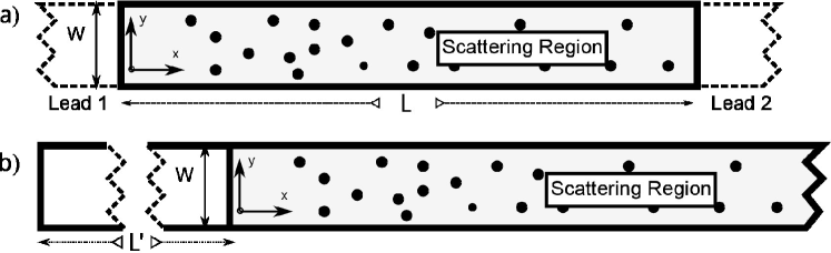
Figure 1: The multichanneled nanowire of width $W$, which is an RSW topological superconductor with a Gaussian disorder having an average value $\left\langle V\right\rangle=0$. a) In the leads, we take $\alpha_{\textrm{SO}}$, $\Delta$ and $V(x,y)$ to be zero, making the leads metallic. Our analytical results assume a semi-infinite wire ($L\rightarrow\infty$), whereas in our numerical full tight-binding calculations we use wires of length $L\gg l_{\text{MFP}},\xi,l_{\textrm{SO}}$. b) The form of the wire used to construct the Majorana solutions in section II.1. The part of the wire left of the scattering region is again metallic.

In this section, we investigate the topological properties of multichanneled topological superconductor nanowires. Such wires are experimentally realized by proximity coupling a semiconductor nanowire with Rashba spin-orbit interaction to an s-wave superconductor (RSW, see Fig. 1 (a)). The quasiparticles in RSW nanowires are described by the following Bogoliubov–de Gennes (BdG) Hamiltonian: REF:Lutchyn10 ; REF:Oreg10 ; REF:deGennes99

$$H =\int\Psi^{\dagger}\,\mathcal{H}_{\mathrm{BdG}}\,\Psi\,d\mathbf{r}$$

$$\mathcal{H}_{\mathrm{BdG}} =\left(h_{0}+\alpha_{\textrm{SO}}(\mathbf{p}\times\mathbf{\sigma})\right)\tau_{z}+B\sigma_{x}+\Delta\tau_{x},$$ (1)

where $h_{0}=\varepsilon(p)+V(\mathbf{r})$, $\Psi^{\dagger}=[\psi_{\uparrow}^{\dagger},\psi_{\downarrow}^{\dagger},\psi_{\downarrow},-\psi_{\uparrow}]$ is the Nambu spinor with $\psi_{\uparrow(\downarrow)}$ being the destruction operator for an electron with spin up(down). The kinetic energy term $\varepsilon(p)$ is given by $\frac{\mathbf{p}^{2}}{2m}-\mu$ in a continuum system. We consider a 2D wire with $\mathbf{p}=(p_{x},p_{y})$. The on-site potential is given by $V(\mathbf{r})$, $\mu$ is the chemical potential measured from the bottom of the band, $\alpha_{\textrm{SO}}$ is the spin-orbit coupling (SOC) strength, $B$ is the Zeeman field and $\Delta$ is the proximity-induced s-wave superconducting gap. The Pauli matrices $\sigma_{i}$ ($\tau_{i}$) act on the spin (electron-hole) space.

In the limit of large $B$, the wire is completely spin polarized. Then the low-energy quasiparticles are described by an effective p-wave Hamiltonian as discussed in previous literature. REF:Adagideli14 ; REF:Akhmerov11 ; REF:Brouwer11b ; REF:DeGottardi13a ; REF:Fulga11 ; REF:Hui14a ; REF:Lobos12 ; REF:Rieder13 ; REF:Potter11a ; REF:Potter11b ; REF:Rieder12 ; REF:Sau12 ; REF:Sau13 For completeness, we discuss this limit in Appendix D.

The Hamiltonian in Eq. (II) is in the Altland-Zirnbauer (AZ) symmetry class D (class D for short) in two dimensions REF:Altland97 with a topological number $Q_{\textrm{D}}\in\mathbb{Z}_{2}$ . In the absence of SOC along the $y$-direction, i.e. when the $\alpha_{\textrm{SO}}\,p_{y}\,\sigma_{x}\tau_{z}$ term is set to zero, this Hamiltonian also possesses a chiral symmetry, placing it into AZ symmetry class BDI (class BDI for short) with an integer topological number $Q_{\textrm{BDI}}\in\mathbb{Z}$. REF:Tewari12 ; REF:Rieder13 In the thin wire limit, i.e. $W\ll l_{\textrm{SO}}$, chiral symmetry breaking terms are $\mathcal{O}\left((W/l_{\textrm{SO}})^{2}\right)$. Hence, the system in Eq. (II) has an approximate chiral symmetry. REF:Rieder12 ; REF:Tewari12 ; REF:Diez12 We show in the next section that the class-BDI (chiral) topological number $Q_{\textrm{BDI}}\in\mathbb{Z}$ and the class-D topological number are related as $Q_{\textrm{D}}=(-1)^{Q_{\textrm{BDI}}}$ (see Eq. (7)). REF:Fulga11

II.1 Topological index for a disordered multichannel s-wave wire

To obtain the relevant topological index that counts the number of the Majorana end states for a RSW wire with disorder, we start with the BdG Hamiltonian $\mathcal{H}_{\mathrm{BdG}}$ in Eq. (II). Following Adagideli et al., REF:Adagideli14 we perform the unitary transformation $\mathcal{H}_{\mathrm{BdG}}\rightarrow\mathcal{H}_{\mathrm{BdG}}^{\prime}=\mathcal{U}^{\dagger}\mathcal{H}_{\mathrm{BdG}}\mathcal{U}$, where $\mathcal{U}=(1+i\sigma_{x})(1+i\tau_{x})\left[1+\sigma_{z}+(1-\sigma_{z})\tau_{x}\right]/4$. Having thus rotated the Hamiltonian to the basis that off-diagonalizes its dominant part and leaves the small chiral symmetry breaking terms $\tau_{z}\sigma_{z}$ in the diagonal block, we obtain

$$\mathcal{H}_{\mathrm{BdG}}^{\prime} =-\tau_{y}\left(\sigma_{z}\,h_{0}+\alpha_{\textrm{SO}}\,p_{x}\right)+\tau_{x}\left(B\,\sigma_{x}+\Delta\right)$$

$$\quad+\,\tau_{z}\sigma_{y}\,\alpha_{\textrm{SO}}\,p_{y}\,.$$ (2)

We first set the chiral symmetry breaking term $\tau_{z}\,\sigma_{y}\,\alpha_{\textrm{SO}}\,p_{y}$ to zero and focus on $E=0$. The eigenvalue equation then decouples into the upper and lower spinor components. The solutions are of the form $\chi_{+}=(\phi_{+},0)^{T}$ and $\chi_{-}=(0,\phi_{-})^{T}$ where $\phi_{\pm}$ obey the following equation:

$$\left(\varepsilon(p)\sigma_{z}-i\,p_{x}\alpha_{\textrm{SO}}\sigma_{x}\mp B\mp\Delta\sigma_{x}\right)\,\phi_{\pm} =0.$$ (3)

Here, we have performed an additional rotation $\sigma_{z}\rightarrow\sigma_{y}$, $\sigma_{y}\rightarrow-\sigma_{z}$ and premultiplied with $\pm\sigma_{x}$. We note that the operator acting on $\phi_{\pm}$ is not Hermitian.

We now perform a gauge transformation $\phi_{\pm}(x,y)\rightarrow e^{-\kappa_{\alpha}x}\phi_{\pm}(x,y)$ with a purely imaginary parameter $i\kappa_{\alpha}$. We take $\kappa_{\alpha}$ to be of first order in $\alpha_{\textrm{SO}}$ and identify the following terms in the nonhermitian operator in Eq. (3) in order of increasing power of $\alpha_{\textrm{SO}}$:

$$H_{0} =h_{0}(p;x,y)\sigma_{z}\mp B\mp\Delta\sigma_{x}$$

$$H_{1} =\frac{i\hbar\kappa_{\alpha}p_{x}}{m}\sigma_{z}-i\alpha_{\textrm{SO}}p_{x}\sigma_{x}$$

$$H_{2} =-\frac{\hbar^{2}\kappa_{\alpha}^{2}}{2m}\sigma_{z}+\hbar\alpha_{\textrm{SO}}\kappa_{\alpha}\sigma_{x},$$ (4)

where we have indicated the $(x,y)$ dependence of $h_{0}(p;x,y)$ through the potential $V(x,y)$. We absorb $H_{2}$ into $H_{0}$ by redefining $\mu$ and $\Delta$. We now identify $\kappa_{\alpha}$ with the inverse of the effective superconducting length $\xi_{\textrm{eff}}$, setting $\kappa_{\alpha}=\mp\xi_{\textrm{eff}}^{-1}=\mp m\alpha_{\textrm{SO}}\Delta/\hbar\epsilon$ with $\epsilon=\sqrt{B^{2}-\Delta^{2}}$. With this choice, $\{H_{0},H_{1}\}_{+}=0$, which allows us to write the local solutions as follows:

$$\phi_{\pm} =\sum_{n}\xi_{\pm}(\epsilon){\rm e}^{\pm\kappa_{\alpha}x}\big{(}A_{n}f_{n}(x,y;\epsilon)+B_{n}g_{n}(x,y;\epsilon)\big{)}$$

$$\quad+\xi_{\pm}(-\epsilon){\rm e}^{\mp\kappa_{\alpha}x}\big{(}C_{n}f_{n}(x,y;-\epsilon)+D_{n}g_{n}(x,y;-\epsilon)\big{)},$$ (5)

where $\xi_{\pm}(\epsilon)$ are the eigenvectors of the $2\times 2$ matrix $\epsilon\sigma_{z}\mp\Delta\sigma_{x}$ with eigenvalue $\pm|B|$ and $f_{n}$ and $g_{n}$ are the local solutions of the equation $h_{0}\psi=\epsilon\psi$. The presence of a multiple number of local solutions, which is the new aspect of the present problem, reflects the multichannel nature of the wire.

We then consider a semi-infinite wire ($x>0$, $0<y<W$) described by the Hamiltonian in Eq. (II) with Gaussian disorder. After going through the steps described above, we choose without loss of generality $f_{n}$ to be the decaying and $g_{n}$ the increasing function of $x$. We invoke a well known result from disordered multichannel normal state wires and express the asymptotic solutions as $f_{n}=e^{-\Lambda_{n}x}u_{n}(x,y)$ and $g_{n}=e^{\Lambda_{n}x}v_{n}(x,y)$ where $u_{n}(x,y),v_{n}(x,y)$ are ${\cal O}(1)$ functions as $x\rightarrow\infty$ and $\Lambda_{n}>0$ are the Lyapunov exponents. REF:Beenakker97 ; REF:Fulga11 ; REF:DeGottardi13a ; REF:Rieder13 ; REF:Adagideli14

We now focus on a tight-binding system, where the number of Lyapunov exponents $N_{\textrm{max}}$ is finite. (In the continuum limit, we have $N_{\textrm{max}}\rightarrow\infty$.) For the boundary conditions at $x=0$, we first extend the hardwall back to $x=-L^{\prime}$ with $L^{\prime}$ a small value, and consider a normal metal in the strip $-L^{\prime}<x<0$ and $0<y<W$ (see Figure 1 (b); in Eq. (II), $\alpha_{\textrm{SO}}=0$, $\Delta=0$, $V(x,y)=0$). The hardwall boundary condition at $x=-L^{\prime}$ can be expressed as $\underline{\underline{R}}\cdot\underline{b}_{+}=\underline{b}_{-}$ with $\underline{b}_{+}\equiv(\ldots,A_{n},C_{n},\ldots)^{T}$, $\underline{b}_{-}\equiv(\ldots,B_{n},D_{n},\ldots)^{T}$ and $\underline{\underline{R}}$ as the extended reflection matrix. REF:Mello04 We therefore have $2N_{\textrm{max}}$ boundary conditions, leaving $2N_{\textrm{max}}$ of the $4N_{\textrm{max}}$ parameters undetermined.

The boundary conditions at $x\rightarrow\infty$ require that $\phi_{\pm}$ have only exponentially decaying solutions. We focus on the $B>\Delta$ case, yielding real $\kappa_{\alpha}$ and $\epsilon$. (As discussed in References REF:Sau10 and REF:Oreg10 , the $B<\Delta$ case yields no solutions.) We take $\kappa_{\alpha}>0$ for definiteness. (The following arguments can be extended trivially to the $\kappa_{\alpha}<0$ case.) The exponential asymptotic factors in the solutions contain a factor of $e^{\pm\kappa_{\alpha}x}$ in various sign combinations, affecting the overall convergence at $x\rightarrow\infty$. In particular, the solutions $\phi_{+}$ have exponential factors of $e^{(\kappa_{\alpha}-\lambda_{n}(\epsilon))x}$, $e^{(\kappa_{\alpha}+\lambda_{n}(\epsilon))x}$, $e^{(-\kappa_{\alpha}-\lambda_{n}(-\epsilon))x}$ and $e^{(-\kappa_{\alpha}+\lambda_{n}(-\epsilon))x}$, whereas the $\phi_{-}$ solutions have the same form of exponential factors with the sign of $\kappa_{\alpha}$ switched. For $|\kappa_{\alpha}|$ smaller than all Lyaponov exponents, all $B_{n}$ and $D_{n}$ are set to zero as they would represent diverging solutions at $x\rightarrow\infty$. There are therefore $2N_{\textrm{max}}$ more conditions , bringing the total up to $4N_{\textrm{max}}$, to determine a total of $4N_{\textrm{max}}$ parameters, yielding only accidental solutions. However, for a given $n=n_{*}$, if $\textrm{min}\,(\lambda_{n_{*}}(\epsilon),\lambda_{n_{*}}(-\epsilon))<\kappa_{\alpha}<\textrm{max}\,(\lambda_{n_{*}}(\epsilon),\lambda_{n_{*}}(-\epsilon))$, there are three growing solutions for one of the $\phi_{\pm}$ sectors and only one for the other sector. (If $\lambda_{n_{*}}(\epsilon)<\lambda_{n_{*}}(-\epsilon)$, the $\phi_{+}$ sector has the three growing solutions and vice versa.) The sector with three growing solutions thus has the number of boundary conditions increased by one and the other sector has the number of boundary conditions decreased by one. If any sector has more than $4N_{\textrm{max}}$ boundary conditions in total, then there are no solutions for that sector. Therefore, the BDI topological number $Q_{\textrm{BDI}}\in\mathbb{Z}$ is given by the number of free parameters, which is equal to $4N_{\textrm{max}}$ minus the total number of equations arising from the boundary condition at $x=-L^{\prime}$. We obtain:

$$Q_{\textrm{BDI}} =\sum_{n}\Theta\left(\xi_{\text{eff}}^{-1}-\Lambda_{n}(\epsilon)\right)\,\Theta\left(\Lambda_{n}(-\epsilon)-\xi_{\text{eff}}^{-1}\right)$$

$$\quad-\sum_{n}\Theta\left(\xi_{\text{eff}}^{-1}-\Lambda_{n}(-\epsilon)\right)\,\Theta\left(\Lambda_{n}(\epsilon)-\xi_{\text{eff}}^{-1}\right).$$ (6)

We see that each Lyapunov exponent pair $\Lambda_{n}(\pm\epsilon)$ contributes a topological charge $Q^{(n)}_{\textrm{BDI}}$ to the overall topological charge. Hence $Q_{\textrm{BDI}}=\sum_{n}Q^{(n)}_{\textrm{BDI}}$, where

$$Q^{(n)}_{\textrm{BDI}}=\begin{cases}+1\quad\textrm{if }\Lambda_{n}(-\epsilon)>\xi_{\textrm{eff}}^{-1}>\Lambda_{n}(\epsilon)\\ -1\quad\textrm{if }\Lambda_{n}(-\epsilon)<\xi_{\textrm{eff}}^{-1}<\Lambda_{n}(\epsilon)\\ {\phantom{+}}0\quad\textrm{otherwise.}\end{cases}$$

We thus generalize the resuls of Ref. REF:Adagideli14 to a multichannel RSW wire. We note, however, that the total number of Majorana end states for a multichannel RSW wire in class BDI, given by $|Q_{\textrm{BDI}}|$, is not equal to sum of the Majorana states per Lyapunov exponent pair, i.e. $|Q_{\textrm{BDI}}|\neq\sum_{n}|Q^{(n)}_{\textrm{BDI}}|$.

We now consider the full Hamiltonian in Eq. (II) with the chiral symmetry breaking term included. This Hamiltonian in two dimensions is in class D and only approximately in class BDI. The chiral symmetry breaking term pairwise hybridizes the Majorana states described above, moving them away from zero energy. However, because of the particle-hole symmetry in the topological superconductor, any disturbance or any perturbation that is higher order in $\alpha_{\textrm{SO}}$ can only move the solutions away from zero energy eigenvalue in pairs; i.e. for any solution moving away from zero eigenvalue towards a positive value, a matching solution must move to a negative eigenvalue. Therefore, the number of zero eigenvalue solutions changes in pairs. Hence, the parity doesn’t change. The parity changes, however, every time one of the Lyapunov exponents passes through the value of $\xi_{\text{eff}}^{-1}$. We therefore arrive at the class D topological index $Q_{\textrm{D}}=(-1)^{Q_{\textrm{BDI}}}$ as REF:Fulga11

$$Q_{\textrm{D}} =\prod_{n,\pm}{\rm sgn}\big{(}\Lambda_{n}(\pm\epsilon)\,\xi_{\text{eff}}-1\big{)},$$ (7)

indicating that there’s a class D Majorana solution at zero energy ($Q_{\textrm{D}}=-1$) if there are an odd number of BDI Majorana states per edge. Therefore, for the topological state of the RSW wire to change from trivial to nontrivial or vice versa, it is necessary and sufficient to have $Q_{\textrm{BDI}}$ described in Eq. (II.1) change by one. The above equation thus constitutes the multichannel generalization of Eq.(7) of Ref. REF:Adagideli14 .

To calculate the topological index $Q_{\textrm{D}}$ in Eq. (7), we relate the Lyapunov exponents in Eq. (II.1) to transport properties, namely the mean free path, of a disordered wire. We first note that as $L\rightarrow\infty$, the Lyapunov exponents $\Lambda_{n}$ are self-averaging, with a mean value $\bar{\Lambda}_{n}$ given by

$$\bar{\Lambda}_{n}(\mu_{\textrm{eff}}) =\frac{n}{(\bar{N}(\mu_{\textrm{eff}})+1)\,l_{\text{MFP}}}$$ (8)

where $\mu_{\textrm{eff}}=\mu\pm\epsilon$, $\bar{N}(\mu_{\textrm{eff}})=\lfloor Wk_{F}(\mu_{\textrm{eff}})/\pi\rfloor$, $k_{F}=\sqrt{2m\mu_{\textrm{eff}}/\hbar^{2}}$, $n\in 1\ldots\bar{N}(\mu_{\textrm{eff}})$ and $l_{\text{MFP}}$ is the MFP of the disordered wire. REF:Beenakker97 We use Fermi’s Golden Rule to approximate the mean free path $l_{\textrm{MFP}}$ by calculating the lifetime of a momentum state and multiplying it with the Fermi speed. We obtain, for a quadratic dispersion relation $\varepsilon(p)=p^{2}/2m-\mu$,

$$l_{\text{MFP}}^{-1} =\frac{4m^{2}\gamma}{\hbar^{4}\pi k_{F}}\,\zeta_{N}^{-1},$$ (9)

where $\zeta_{N}^{-1}$ is a dimensionless number whose detailed form is given in Eq. (17). The details of this calculation can be found in Appendix A.

In order to compare our numerical tight-binding results with the analytical results obtained through Eq. (7) and (II.1), we also calculate the mean free path $l_{\text{MFP}}^{\text{TB}}$ for a tight-binding (TB) dispersion relation $\varepsilon(k_{x,n})=2t\,\left(2-\cos{(k_{x,n}a)}-\cos{(n\pi a/W)}\right)$, where $t$ is the hopping parameter, $a$ is the lattice parameter for the TB lattice, $W$ is the width of the lattice and $k_{x,n}$ is defined through $k_{x,n}^{2}+k_{y,n}^{2}=k_{F}^{2}$ with $k_{y,n}=n\pi/W$. We obtain

$$(l_{\text{MFP}}^{\text{TB}})^{-1} =\frac{\gamma}{\bar{N}^{\textrm{TB}}Wa^{2}t^{2}}\,(\zeta_{N}^{\text{TB}})^{-1}.$$ (10)

where $\bar{N}^{\textrm{TB}}$ is given by $\lfloor(W/\pi a)\arccos{(1-\varepsilon/2t)}\rfloor$ for $0<\varepsilon<4t$ and $\lfloor(W/\pi a)\arccos{(1-(4-\varepsilon/2t))}\rfloor$ for $4t<\varepsilon<8t$. The details of the calculation and the dimensionless constant $\zeta_{N}^{\text{TB}}$ are again found in Appendix A.

The topological phase boundaries, shown in Figures 2 and 3 as the bold black lines, are calculated by equating $\xi^{-1}$ to $\Lambda_{n}$ obtained from Eq. (8) and (10). We thus obtain the critical field $B^{*}$ at which the system goes through a topological phase transition via thie following implicit equation:

$$B^{*} =\Delta\,\sqrt{\beta\,\Gamma_{n}^{\textrm{TB}}\left(\mu_{\textrm{eff}}(B^{*})\right)+1}$$ (11)

where $\beta=(Wa^{2}t^{2}/\gamma l_{\textrm{SO}})^{2}$, $\mu_{\textrm{eff}}(B^{*})=\mu\pm\sqrt{(B^{*})^{2}+\Delta^{2}}$ and

$$\Gamma_{n}^{\textrm{TB}}\left(\mu_{\textrm{eff}}\right) =\left(\frac{\bar{N}^{\textrm{TB}}\left(\mu_{\textrm{eff}}\right)}{n}\right)^{2}$$

$$\qquad\times\left(\zeta_{N}^{\text{TB}}\left(\mu_{\textrm{eff}}\right)\right)^{2}\left(\bar{N}^{\textrm{TB}}\left(\mu_{\textrm{eff}}\right)+1)\right)^{2}.$$

Equation (11) constitutes the central finding of our paper. It is an analytical expression that determines all topological phase boundaries of a multichannel disordered wire.

An experimentally interesting point is the largest values of various system parameters that allow a topological transition. Using Equations (II.1) and (7), we estimate the upper critical field $B^{*}|_{\gamma}\,$, i.e. the minimum value of $B$ above which the system is always in a topologically trivial state at a given disorder strength $\gamma$, as

$$B^{*}|_{\gamma} \sim\Delta\,\frac{l_{\textrm{tr}}^{\textrm{max}}}{l_{\textrm{SO}}},$$ (12)

where $l_{\textrm{tr}}^{\textrm{max}}=\textrm{max}(\{\Lambda_{n}^{-1}\})$ is the maximum localization length achievable in the system. For a fixed nonzero disorder, $B^{*}|_{\gamma>0}$ is infinite for a continuum system as the localization length increases indefinitely with increasing Fermi energy. For a TB system, the upper critical field $B^{*}|_{\gamma>0}$ is finite because the localization length is bounded in TB systems. For a clean wire, $B^{*}|_{\gamma=0}$ is infinite for both the TB and the continuum models.

II.2 Numerical simulations

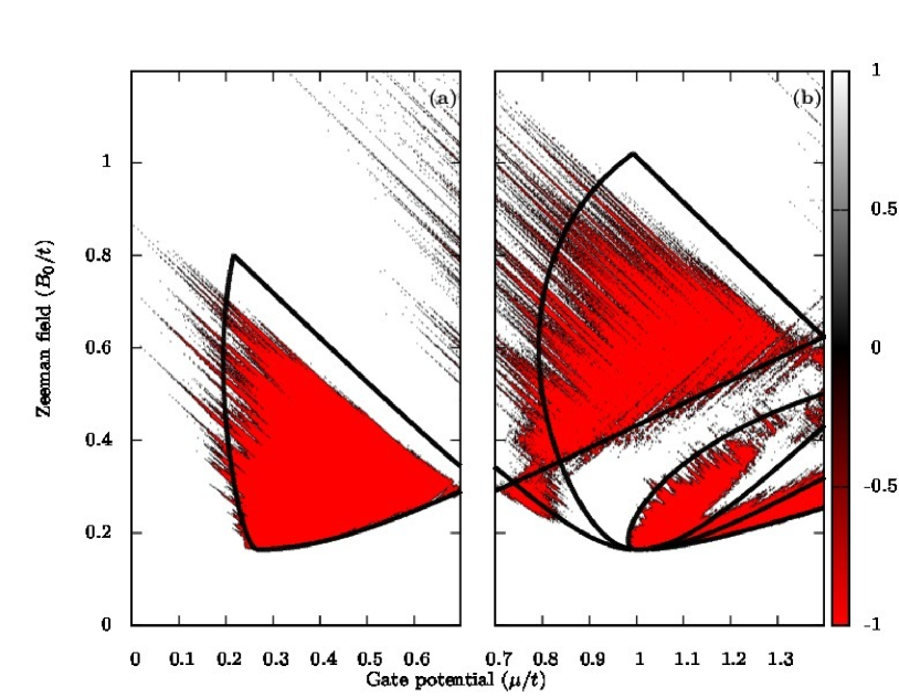
Figure 2: (Color online) $\mu$ vs. $B$ vs. $Q_{\textrm{D}}$ for a five-channel system (compare with Figs. 8 and 7.) The background red-white colors are obtained using a numerical tight-binding simulation with $L=30000a$ and $W=5a$, while the black lines, which represent the topological phase boundaries, are obtained analytically using Eq. (7). Here, $V_{0}=\sqrt{\gamma/a^{2}}=0.2t$, $\alpha_{\textrm{SO}}=0.02\hbar/ma$ ($l_{\textrm{SO}}=4.08\mu m$) and $\Delta=0.164t$, where $t=\hbar^{2}/2ma^{2}$ and $a=0.01l_{\textrm{SO}}$ is the tight-binding lattice spacing. The fragmented nature of the topological phase diagram seen in (b) cannot be explained in a p-wave picture. See Appendix B for a discussion of corresponding experimental parameters.

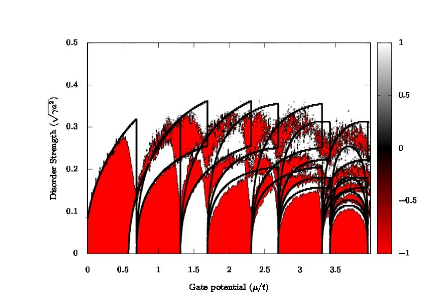
Figure 3: (Color online) $\mu$ vs. $V_{0}=\sqrt{\gamma/a^{2}}$ vs. $Q$ for a multichannel RSW wire. The black lines, which represent topological phase boundaries, are obtained analytically using Eq. (7). The background red-white colors are obtained using tight-binding numerical simulations with $L=60000a$. In both cases, $W=4a$, $\alpha_{\textrm{SO}}=0.015\hbar/ma$, $\Delta=0.20t$ and $B=0.35t$, where $t=\hbar^{2}/2ma^{2}$ is the tight-binding hopping parameter and $a$ is the TB lattice spacing. See Appendix B for a discussion of corresponding experimental parameters.

In this section, we obtain the topological index of a disordered multichannel wire numerically and compare it with our analytical results from the previous section. For our numerical simulations, we take the TB form of the Hamiltonian in Eq. (II) whose details can be found in the Appendix B. We consider a wire of length $L\gg l_{\text{MFP}}$, $\xi$ or $\l_{\textrm{SO}}$, with metallic leads ($\alpha_{\textrm{SO}}=0$, $\Delta=0$ and $V(x,y)=0$ in the leads). We use the results of Fulga et al. to obtain the topological quantum number of the disordered multichannel wire from the scattering matrices of the wires. REF:Fulga11 For a semi-infinite wire in the symmetry class D, the topological charge is given by $Q_{\textrm{D}}=\text{det}(r)$ where $r$ is the reflection matrix. For a quasiparticle insulator, this determinant can only take the values $\pm 1$. However, for a finite system this determinant can in general have any value in the $[-1,1]$ interval. We obtain the reflection matrix of the TB system in our numerical TB simulations using the Kwant library REF:Kwant14 and then use this relation to calculate $Q_{\textrm{D}}$. We plot the topological phase diagram in Figures 2 and 3, where the red and white colors represent $Q_{\textrm{D}}=-1$ and $Q_{\textrm{D}}=+1$ respectively.

Figure 2 exemplifies our central result given in Eq. (11). We find that for a nearly depleted wire (Fig. 2a), the topological phase merely shifts to the higher values of the chemical potential in agreement with Ref. REF:Adagideli14 . For higher chemical potentials/doping, we observe a fragmented topological phase diagram (Fig. 2b). We find good agreement with our analytical results from Eq. (11). We note in passing that, this fragmentation cannot be explained by a simple p-wave picture as these topological phases arise despite the incomplete spin-polarization of the wire under a low magnetic field. For a full phase diagram over the entire bandwidth, but for slightly different material parameters, see Figure 8, where the reentrant phases are apparent.

In Fig. 3, we plot the topological number $Q_{\textrm{D}}$ as a function of $\mu$ and the disorder strength $\sqrt{\gamma/a^{2}}$ for a constant $B_{\textrm{Zeeman}}$ over the full TB bandwidth. The reentrant nature of the topological phase diagram can also be seen in this plot, for example, by following the $\mu=1.5$ line as $\gamma$ is increased. As the disorder strength increases, series of topological transitions occur, similar to the PW wire. REF:Rieder13 However, unlike the PW wire, the number of transitions is given by $\bar{N}(\mu+\epsilon)+\bar{N}(\mu-\epsilon)$ rather than $\bar{N}(\mu)$, with $\bar{N}(\mu)$ defined as $\bar{N}(\mu_{\textrm{eff}})=\lfloor Wk_{F}(\mu_{\textrm{eff}})/\pi\rfloor$. For further discussion of the emergence of effective p-wave picture at high magnetic fields, see Appendix C.

III Conclusion

In summary, we investigate the effect of disorder in multichannel Rashba SOC proximity-induced topological superconductor nanowires (RSW nanowires) at experimentally relevant parameter ranges. We derive formulae that determine all topological phase boundaries of a multichannel disordered RSW wire. We test these formulae with numerical tight-binding simulations at experimentally relevant parameter ranges and find good agreement without any fitting parameters. We show that there are additional topological transitions for the RSW wires leading to a richer phase diagram with further fragmentalization beyond that of the p-wave models.

Appendix A Mean free path

We consider a long wire along the $x$-axis, having a length of $L$ along the $x$-direction and a width of $W$ along the $y$-direction and metallic leads at the end, with a Gaussian disorder of the form $\left\langle V(\mathbf{r})\,V(\mathbf{r}^{\prime})\right\rangle=\gamma\,\delta(\mathbf{r}-\mathbf{r}^{\prime})$. We obtain the ensemble average of the matrix element between the $n^{\text{th}}$ and $l^{\text{th}}$ transverse channels as $\boldsymbol{k}(k_{x},n)\rightarrow\boldsymbol{k}^{\prime}(k_{x}^{\prime},l)$ as

$$\left\langle|V_{kk^{\prime}}|^{2}\right\rangle =\frac{\gamma}{LW}\left(1+\frac{\delta_{n,l}}{2}\right).$$ (13)

We then use Fermi’s Golden Rule to calculate the inverse lifetime of a momentum state $k$, $\tau_{k\rightarrow k^{\prime}}^{-1}$:

$$\left\langle l_{\text{MFP}(k_{x},n\rightarrow k_{x}^{\prime},l)}^{-1}\right\rangle =\left(\frac{1}{\hbar}\,\frac{\partial\,\varepsilon_{k}}{\partial k_{x}}\right)^{-1}\times\frac{2\pi}{\hbar}\,\frac{\gamma}{LW}\times$$

$$\qquad\left(1+\frac{\delta_{n,l}}{2}\right)\,\rho(\varepsilon_{k^{\prime}}).$$ (14)

where $\varepsilon_{k}$ gives the dispersion relation and $\rho(\varepsilon_{k})$ is the density of states. We then sum over the initial and final states $k^{\prime}$ in Eq. (A) to obtain the total inverse MFP:

$$\left\langle l_{\text{MFP}}^{-1}\right\rangle =\sum_{k_{x},k_{y};k^{\prime}_{x},k^{\prime}_{y}}\left\langle l_{\text{MFP}(k_{x},n\rightarrow k_{x}^{\prime},l)}^{-1}\right\rangle$$ (15)

We first apply Eq. (15) to a free electron dispersion of the form $\varepsilon(k)=\hbar^{2}k^{2}/2m=\hbar^{2}/2m\,(k_{n,x}^{2}+n^{2}\pi^{2}/W^{2})$ for $n\in{1,\ldots,\bar{N}}$ where $\bar{N}(\mu_{\textrm{eff}})=\lfloor Wk_{F}(\varepsilon)/\pi\rfloor$. The resulting total ensemble-averaged inverse MFP is

$$\left\langle l_{\text{MFP}}^{-1}\right\rangle =\sum_{n=1}^{\bar{N}}\sum_{l=1}^{\bar{N}}\int\frac{dk^{\prime}_{n,x}}{\pi/L}\,\frac{m^{2}}{\hbar^{4}}\frac{2\gamma W}{L\pi}\,\left(1+\frac{\delta_{nl}}{2}\right)\,\frac{\pi}{W}\times$$

$$\qquad\frac{\delta(k^{\prime}_{l,x}\pm\sqrt{2m\varepsilon/\hbar^{2}-l^{2}\pi^{2}/W^{2}})}{\sqrt{2m\varepsilon/\hbar^{2}-n^{2}\pi^{2}/W^{2}}\,\sqrt{2m\varepsilon/\hbar^{2}-l^{2}\pi^{2}/W^{2}}}$$

$$=\frac{4m^{2}\gamma}{\hbar^{4}\pi k_{F}}\,\zeta_{N}^{-1},$$ (16)

where $k_{F}=\sqrt{2m\varepsilon/\hbar^{2}}$ is the Fermi wavevector,

$$\zeta_{N}^{-1} =\frac{3\bar{N}}{2}\sum_{n=1}^{\bar{N}}\eta_{n}^{2}+2{\bar{N}}\sum_{n=1}^{\bar{N}}\sum_{l>n}^{\bar{N}}\eta_{n}\,\eta_{l},$$ (17)

and $\eta_{n}=\left(\frac{W^{2}k_{F}^{2}}{\pi^{2}}-n^{2}\right)^{-\frac{1}{2}}$, in agreement with Eq.(8) in the supporting online material of Rieder et al. REF:Rieder13 . The value of $\zeta_{N}$ just below the transition $N\rightarrow N+1$ (denoted $\zeta_{N\rightarrow N+1}$) is plotted in Figure 4.

Figure 4: $\zeta_{N\rightarrow N+1}^{-1}/(N+1)$ vs. $N$.

We now derive the MFP for a TB dispersion relation given by

$$\varepsilon(k_{x,n}) =2t\,\left(2-\cos{(k_{x,n}a)}-\cos{(n\pi a/W)}\right).$$ (18)

The number of channels is given by $\bar{N}=\lfloor(W/\pi a)\arccos{(1-\varepsilon/2t)}\rfloor$ for $0<\varepsilon<4t$ and by $\bar{N}=\lfloor(W/\pi a)\arccos{(1-(4-\varepsilon/2t))}\rfloor$ for $4t<\varepsilon<8t$. The resulting disorder-averaged inverse MFP reads:

$$\left\langle(l_{\text{MFP}}^{\text{TB}})^{-1}\right\rangle =\frac{\gamma}{\bar{N}Wa^{2}t^{2}}\,(\zeta_{N}^{\text{TB}})^{-1}$$ (19)

where the dimensionless $(\zeta_{N}^{\text{TB}})^{-1}$ is given by

$$(\zeta_{N}^{\text{TB}})^{-1} =\frac{3\bar{N}}{2}\sum_{n=1}^{\bar{N}}(\eta_{n}^{\text{TB}})^{2}+$$

$$\qquad 2\bar{N}\sum_{n=1}^{\bar{N}}\sum_{l>n}^{\bar{N}}\eta_{n}^{\text{TB}}\eta_{l}^{\text{TB}}.$$ (20)

Here, $\eta_{n}^{\text{TB}}=|\sin{(k_{x,n}\,a)}|^{-1}$ and $\sin{(k_{x,n})}$ is obtained using Eq. (18)

Appendix B Numerical tight-binding simulations

We start by obtaining the TB form of the RSW BdG Hamiltonian REF:deGennes66 in Eq. (II) in the usual way using finite differences (see, for example, Ref.REF:Lutchyn10 ,REF:Oreg10 ,REF:Stanescu11 ,REF:Datta97 ). It reads:

$$\mathcal{H}_{\mathrm{BdG}}^{\mathrm{TB}} =\left[\left(4t+V(x,y)-\mu(x,y)\right)\,\tau_{z}+B_{\textrm{Z}}\,\sigma_{z}\right.$$

$$\quad+\,\left.\Delta(x,y)\,\tau_{x}\right]\,\left|{x,y}\right\rangle\left\langle{x,y}\right|$$

$$\quad+\,\left[-t\,\tau_{z}-\frac{i}{2}\alpha_{\textrm{SO}}(x,y)\,\tau_{z}\,\sigma_{y}\right]\,\left|{x+a,y}\right\rangle\left\langle{x,y}\right|$$

$$\quad+\,\left[-t\,\tau_{z}+\frac{i}{2}\alpha_{\textrm{SO}}(x,y)\,\tau_{z}\,\sigma_{x}\right]\,\left|{x,y+a}\right\rangle\left\langle{x,y}\right|$$

$$\quad+\mathrm{h.c.}$$ (21)

where $t=\hbar^{2}/2ma^{2}$ is the hopping parameter, $V(x,y)$ is the Gaussian random potential, $\mu(x,y)$ is the relevant gate potential, $B_{\textrm{Z}}$ is the Zeeman field, $\Delta(x,y)$ is the s-wave superconducting pairing (taken to be real), $\alpha_{\textrm{SO}}(x,y)$ is the effective Rashba SOC due to proximity effect and $a$ is the lattice constant for the TB lattice. Here, $V(x,y)$, $B_{\textrm{Z}}$, $\Delta(x,y)$ and $\alpha_{\textrm{SO}}(x,y)$ are nonzero only within the scattering region. $B_{\textrm{Z}}$, $\alpha_{\textrm{SO}}(x,y)$ and $\Delta(x,y)$ are constant within the scattering region except for the values of $\alpha_{\textrm{SO}}(x,y)$ in the scattering region-lead boundary, where we take it to be half of its value in the bulk.

The experimental values for InSb nanowires quoted in Mourik et al. REF:Mourik12 are $\alpha_{\textrm{SO}}=0.2\,\textrm{eV}\textup{\AA}$, $l_{\textrm{SO}}\sim 2000\textup{\AA}$, $\Delta=0.25m\textrm{eV}$, $E_{Z}/B=1.5m\textrm{eV}/\textrm{T}$, $m_{*}=0.015m_{e}$ and $\alpha_{\textrm{SO}}^{2}m_{*}/2\hbar^{2}\sim 0.04m\textrm{eV}$. We employ these values verbatim, except for $l_{\textrm{SO}}$ (and correspondingly, $\alpha_{\textrm{SO}}$), for which we use parameters much more accessible experimentally.

We use the Kwant library REF:Kwant14 to obtain the topological phase diagram in our numerical plots. The Kwant library can extract the scattering matrix (S-matrix),REF:Datta97 and therefore the reflection matrix (r-matrix) for a given tight-binding system with leads. The topological index $Q_{\textrm{D}}$ can be obtained from the r-matrix through $Q_{\textrm{D}}=\textrm{det}(r)$ (see Ref. REF:Fulga11 ).

The numerical parameters quoted in the caption of Fig. 2 correspond to $t=1.5m\textrm{eV}$, $a=40.8\textrm{nm}$, $l_{\textrm{SO}}=4.08\mu\textrm{m}$ and $\alpha=6.3\times 10^{-6}\,c$. Disregarding screening, a Zeeman Energy of, say, $0.35t$ on the plot would correspond to a magnetic field $0.35\textrm{T}$, a value easily accessible by the experiment. In Figures 3, 5, 7 and 8 , $l_{\textrm{SO}}=6.0\mu\textrm{m}$, $t=0.7m\textrm{eV}$, $a=60.0n\textrm{m}$ and $\alpha=4.2\times 10^{-6}\,c$. A Zeeman energy of $0.35t$ corresponds to $B=0.17\,\textrm{T}$.

The TB form of the effective PW Hamiltonian of Eq. (23) used in Appendix D is as follows:

$$\mathcal{H}_{\mathrm{PW}}^{\mathrm{TB}} =\left[4t+V(x,y)-\mu(x,y)\right]\,\tau_{z}\,\left|{x,y}\right\rangle\left\langle{x,y}\right|$$

$$\quad+\,\left[-t\,\tau_{z}-\frac{i}{2}\Delta_{\textrm{eff}}(x,y)\,\tau_{x}\right]\,\left|{x+a,y}\right\rangle\left\langle{x,y}\right|$$

$$\quad+\,\left[-t\,\tau_{z}-\frac{i}{2}\Delta_{\textrm{eff}}(x,y)\,\tau_{y}\right]\,\left|{x,y+a}\right\rangle\left\langle{x,y}\right|$$

$$\quad+\mathrm{h.c.}$$ (22)

We use numerical values similar to the RSW case in our PW simulations, except to impose $\Delta_{\textrm{eff}}=\Delta\,\alpha_{\textrm{SO}}/\sqrt{B^{2}-\Delta^{2}}$.

Appendix C Topological phase diagram over the full bandwidth

In this section, we present plots of the topological phase diagram that we obtain analytically from Eq. (7) using a TB dispersion relation (see Section II) over the full bandwidth. Although only the low $\mu$ regions in our plots correspond to experimentally relevant nanowires, the full bandwidth range would be important for systems that are inherently TB, such as atomic chains REF:Nadj-Perge14 or photonic metamaterials REF:Tan14 simulating topological properties. REF:Lu14 All analytical plots are produced using Eq. (7) (Eq. (24) for the PW case), but using a TB dispersion relation for $\epsilon(p)$ in the relevant expressions. All of the numerical results are obtained using a TB simulation utilizing Kwant software, as discussed in the main text.

Figure 5 depicts the analytically calculated topological phase diagram for an RSW wire as a function of $\mu$ and the disorder strength, for various magnetic field strengths. The transition between a RSW wire and a pair of oppositely polarized PW wires can be seen as increasing magnetic field polarizes the system. The topological order is less robust against disorder for higher magnetic fields, because the coherence length becomes longer with increasing $B$. This is the reason why the spin polarized regimes where PW model applies is typically less robust than the lower field regimes where both spin species exist as seen in Fig. 5(a) and 5(c) or (d). In order to complete the discussion, we also present an analytical plot (Figure 6) for an RSW wire for which B is greater than the subband spacing but less than the bandwidth. While this regime is experimentally very hard to achieve, it is useful for comparing the PW and the RSW regimes. The vertical blue line denotes the bottom of the higher energy spin band beyond which both spin species exist. We note that the critical disorder strength increases with the chemical potential, hence spin-polarized regime, which appear at lower chemical potential values, is less robust against disorder.

In Figure 7, the analytically calculated phase diagram of a wire with $W=4a$ is plotted with increasing disorder. We see that the phase diagram gets fragmented as number of channels are increased. We also note that for a given amount of disorder, there is a maximum Zeeman field $B_{\text{max}}$ above which no topological order is present. The reason is that in our numerical TB simulations, the localization length is not a monotonous function of energy. It grows (with increasing energy) until the middle of the band, and after that it decreases as the energy comes closer to the band edge. This places an upper magnetic field limit to topological regions since the superconducting coherence length monotonically increases with $B$. For a pure quadratic dispersion, the upper limit is given by the limitations of the approximations of Fermi’s Golden Rule and would increase indefinitely with increasing energy as discussed in the main text. We note that the upper limit discussed here has a different origin than that discussed by Ref.REF:Rainis13 for finite-length wires.

We finally present the full TB bandwidth version of Fig. 2, with slightly different material properties, here in Fig. 8. This figure is the numerical simulation result that matches the last of the analytical plots in Fig. 7. The relevant numerical values are given in each of the Figures’ captions.

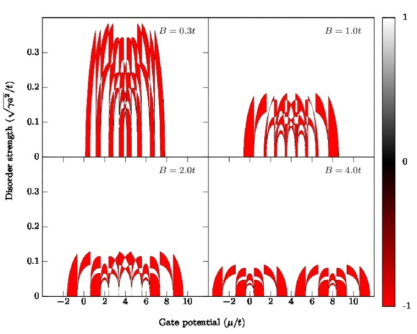
Figure 5: (Color online) $\mu$ vs. $V_{0}=\sqrt{\gamma/a^{2}}$ vs. $Q_{\textrm{D}}$ for a multichanneled RSW wire for different $B$, obtained analytically using Eq. (7). a), b) Low magnetic field $B\gtrsim\Delta$ limit requires a full RSW model and topological order can survive up to high disorder strengths. c), d) The spin-polarized system can be described by a PW model and topological order is completely destroyed with less disorder. Here, $W=4a$, $\alpha_{\textrm{SO}}=0.015\hbar/ma$ and $\Delta=0.20t$ where $t=\hbar^{2}/2ma^{2}$ and $a$ is the tight-binding lattice spacing. See Appendix B for a discussion of corresponding experimental parameters.

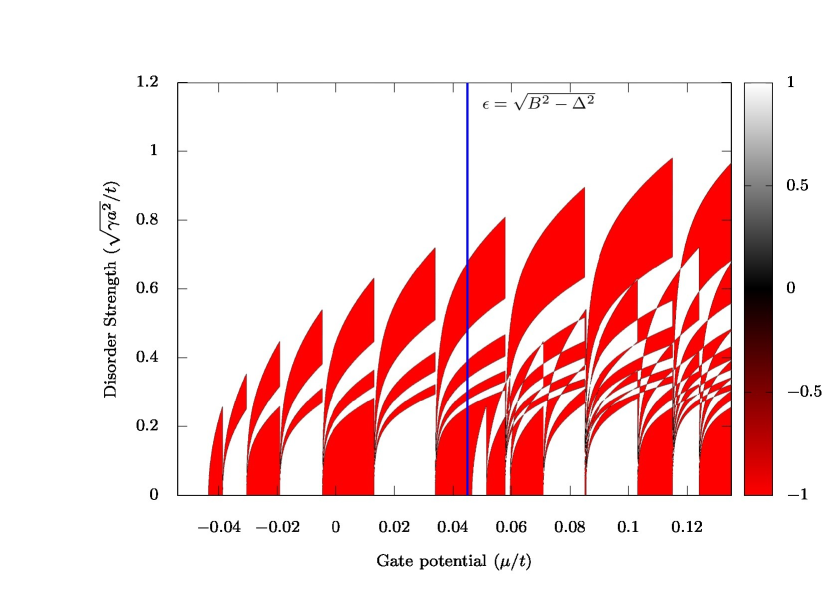
Figure 6: (Color online) $\mu$ vs. $V_{0}=\sqrt{\gamma/a^{2}}$ vs. $Q_{\textrm{D}}$ for a multichanneled wide RSW wire, obtained obtained analytically using Eq. (7), with $W=77a$. Here, $\alpha_{\textrm{SO}}=0.015\hbar/ma$ ($l_{\textrm{SO}}=100a$), $\Delta=0.20t$ and $B=0.205t$ with the hopping parameter $t=\hbar^{2}/2ma^{2}=0.7$ $m$eV and the lattice spacing $a=60$ $n$m. The blue vertical line at $\mu=\epsilon=\sqrt{B^{2}-\Delta^{2}}$ is the bottom of the second spin band.

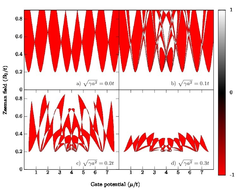
Figure 7: (Color online) $\mu$ vs. $B$ vs. $Q_{\textrm{D}}$ for varying disorder strengths for an RSW TS with Gaussian disorder, analytically calculated using Eq. (7) for a four-channel TB system. Subfigure c) matches the numerical data shown in Fig. 8 . The parameters used are $\alpha_{\textrm{SO}}=0.015\hbar/ma$ and $\Delta=0.2t$, where $t=\hbar^{2}/2ma^{2}$ $a$ is the lattice spacing. See Appendix B for a discussion of corresponding experimental parameters.

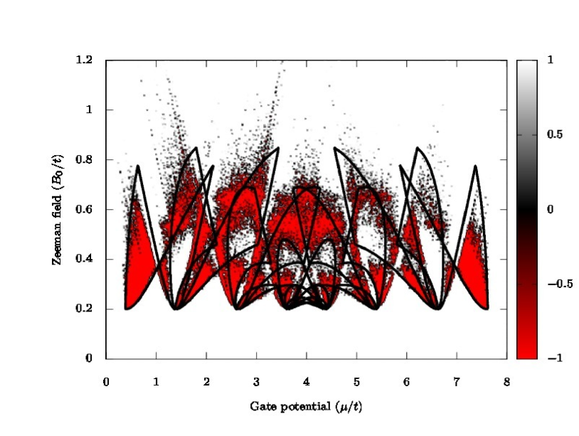
Figure 8: (Color online) $\mu$ vs. $B$ vs. $Q_{\textrm{D}}$ for a four-channel system (compare with Figs. 2 and 7). The black lines, which represent topological boundaries, are obtained analytically using Eq. (7). The background red-white colors are obtained using tight-binding numerical simulations. The parameters are $V_{0}=0.2t$, $\Delta=0.2t$ and $\alpha_{\textrm{SO}}=0.015\hbar/ma$. See Appendix B for a discussion of corresponding experimental parameters.

Appendix D Topological phase diagram for multichannel effective p-wave nanowires with disorder

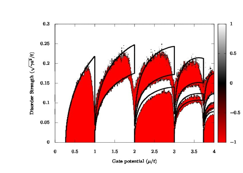
Figure 9: (Color online) $\mu$ vs. $\sqrt{\gamma/a^{2}}$ vs. $Q$ for a multichanneled PW wire with dimensions $W=4a$ and $L=60000a$ ($L$ used only in the numerical tight-binding code) and with $\alpha_{\textrm{SO}}=0.01\hbar/ma$, where $a$ is the tight-binding lattice spacing. The red-white colors in the background are obtained numerically with a tight-binding method whereas the black solid lines are obtained using Eq. (24) with Eq. (10).

In this Appendix section, we present the effects of disorder on PW wires, which is a system previously studied in literature, REF:Adagideli14 ; REF:Akhmerov11 ; REF:Brouwer11b ; REF:DeGottardi13a ; REF:Fulga11 ; REF:Hui14a ; REF:Lobos12 ; REF:Rieder13 ; REF:Potter11a ; REF:Potter11b ; REF:Rieder12 ; REF:Sau12 ; REF:Sau13 for completeness and for comparison with the results of our paper for disordered multichannel RSW nanowires. We start with the Hamiltonian in Eq. (23) and present the topological charge in Eq. (24). We plot the topological phase diagram for a PW wire as a function of $\mu$ and disorder strength for a fixed $B_{\textrm{Zeeman}}$ (Fig. 9) and compare this plot with its analogue for RSW wires (Fig. 3).

The BdG Hamiltonian for an effective p-wave wire with spatially homogeneous effective SOC strength is

$$\mathcal{H}_{\mathrm{BdG}}^{\mathrm{PW}} =\varepsilon(p)\,\tau_{z}+\Delta_{\textrm{eff}}\,\mathbf{p}\cdot\mathbf{\tau}.$$ (23)

Note that $\Delta_{\textrm{eff}}$ has units of velocity while $\Delta$ in Eq. (II) has units of energy. This effective SOC strength is related to the corresponding RSW superconducting gap by $\Delta_{\textrm{eff}}=\Delta\,\alpha_{\textrm{SO}}/\sqrt{B^{2}-\Delta^{2}}$. REF:Lutchyn10 We consider a Gaussian disorder of the form $\left\langle V(\mathbf{r})\,V(\mathbf{r}^{\prime})\right\rangle=\gamma\,\delta(\mathbf{r}-\mathbf{r}^{\prime})$ for $\mathbf{r},\mathbf{r}^{\prime}$ in the wire, with $\gamma$ as the disorder strength and $\left\langle V(\mathbf{r})\right\rangle=0$. This Hamiltonian is useful for comparison with the fully polarized limit of the RSW case.

The Hamiltonian in Eq. (23) is in Altland-Zirnbauer (AZ) symmetry class D in two dimensions REF:Altland97 with a $\mathbb{Z}_{2}$ topological number. This Hamiltonian also possesses a chiral symmetry, broken by the $\Delta_{\textrm{eff}}\,p_{y}\tau_{y}$ term. If this term is set to zero, the Hamiltonian is also in class BDI REF:Rieder12 ; REF:Tewari12 ; REF:Diez12 ; REF:Rieder13 having a $\mathbb{Z}$ topological number. (1D wires trivially satisfy this condition.) In the thin wire limit, i.e. $\Delta_{\textrm{eff}}\ll\hbar/mW$, the chiral symmetry breaking term is $\mathcal{O}\left((m\Delta_{\textrm{eff}}W/\hbar)^{2}\right)$. The wire in class BDI can have an integer number of Majorana fermions at its ends. The chiral symmetry breaking term pairwise hybridizes these solutions. Hence the chiral topological number $Q_{\textrm{BDI}}\in\mathbb{Z}$ and the class-D topological number $Q_{\textrm{D}}\in\mathbb{Z}_{2}$ are related as $Q_{\textrm{D}}={-1}^{Q_{\textrm{BDI}}}$. REF:Fulga11

In order to solve the Schrödinger equation $H\,\Psi=E\,\Psi$ at $E=0$ to obtain the Lyapunov exponents, we follow Adagideli et al. REF:Adagideli14 to off-diagonalize the Hamiltonian and apply an imaginary gauge transformation. This allows us to re-express $Q_{\textrm{BDI}}$ in terms of $\Lambda_{n}$: REF:Rieder13

$$Q_{\textrm{BDI}} =\sum_{n=1}^{\bar{N}}\Theta\left(\xi-\frac{1}{\Lambda_{n}}\right),$$ (24)

where $\bar{N}=\lfloor W/\pi\sqrt{2m\mu/\hbar^{2}}\rfloor$ and $\lfloor x\rfloor$ is the usual floor function. We obtain $\Lambda_{n}$ again using Eq. (8). We obtain $l_{\text{MFP}}^{-1}$ using Fermi’s Golden Rule (see Appendix A) first for a quadratic dispersion relation and then for a TB dispersion relation.

We compare the results found using Eq. 24 with those obtained by numerical simulations in Figure 9 and find an excellent fit over the whole TB bandwidth. In a clean PW wire ($\sqrt{\gamma/a^{2}}=0$), Majorana modes appear if $\bar{N}$ is odd and Majorana states fuse to form ordinary Dirac fermions if $\bar{N}$ is even. This behavior survives up to a finite disorder strength (see Fig. 9). As in the case of RSW wires, further increase of the disorder strength gives a series of transitions between non-trivial and trivial topological phases as each $\Lambda_{n}$ increases and crosses $\xi^{-1}$. While both multichanneled RSW and PW wires feature reentrant behavior, we see that there are additional transitions for the RSW wires leading to a richer phase diagram (compare Figures 9 and 3), in agreement with our analytical results presented in Eq. (11).

References

- (1) M. Z. Hasan and C. L. Kane, Rev. Mod. Phys. 82, 3045 (2010)
- (2) X. L. Qi and S. C. Zhang, Rev. Mod. Phys. 83, 1057 (2011)
- (3) M. Franz and L. Molenkamp, eds., Topological Insulators, 1st ed., Contemporary Concepts of Condensed Matter Science, Vol. 6 (Elsevier, 2013)
- (4) J. Alicea, Rep. Prog. Phys. 75, 076501 (2012)
- (5) M. Leijnse and K. Flensberg, Semicond. Sci. Technol. 27, 124003 (2012)
- (6) C. W. J. Beenakker, Annu. Rev. Condens. Matter Phys. 4, 113 (2013)
- (7) A. Bernevig and T. Hughes, Topological Insulators and Topological Superconductors, 1st ed. (Princeton University Press, 2013)
- (8) S. Elliott and M. Franz, Rev. Mod. Phys. 87, 137 (2015)
- (9) A. Y. Kitaev, Ann. Phys. 303, 2 (2003)
- (10) C. Nayak, S. H. Simon, A. Stern, M. Freedman and S. Das Sarma, Rev. Mod. Phys. 80, 1083 (2008)
- (11) R. Jackiw and P. Rossi, Nucl. Phys. B 190, 681 (1981)
- (12) M. M. Salomaa and G. E. Volovik, Phys. Rev. B 37, 9298 (1988)
- (13) G. Moore and N. Read, Nucl. Phys. B 360, 362–96 (1991)
- (14) N. Read and D. Green, Phys. Rev. B 61, 10267 (2000)
- (15) D. A. Ivanov, Phys. Rev. Lett. 86, 268 (2001)
- (16) A. Y. Kitaev, Phys.-Usp. 44, 131 (2001)
- (17) J. Alicea, Phys. Rev. B 81, 125318 (2010)
- (18) R. M. Lutchyn, J. D. Sau and S. Das Sarma, Phys. Rev. Lett. 105, 077001 (2010)
- (19) J. D. Sau, S. Tewari, R. M. Lutchyn, T. D. Stanescu and S. Das Sarma, Phys. Rev. B 82, 214509 (2010)
- (20) Y. Oreg, G. Refael and F. von Oppen, Phys. Rev. Lett. 105, 177002 (2010)
- (21) Other proposals include REF:Choy11 ; REF:Kjaergaard12 ; REF:Martin12 ; REF:Nadj-Perge13 ; REF:Braunecker13 ; REF:Pientka13a ; REF:Klinovaja13 ; REF:Nakosai13 ; REF:Vazifeh13 ; REF:Kim14 ; REF:Rontynen14 ; REF:Li15 ; REF:Scharf15 .
- (22) V. Mourik, K. Zuo, S. M. Frolov, S. R. Plissard, E. P. A. M. Bakkers and L. P. Kouwenhoven, Science 336, 1003 (2012)
- (23) A. Das, Y. Ronen, Y. Most, Y. Oreg, M. Heiblum and H. Shtrikman, Nat. Phys. 8, 887 (2012)
- (24) M. T. Deng, C. L. Yu, G. Y. Huang, M. Larsson, P. Caroff and H. Q. Xu, Nano Lett. 12, 6414 (2012)
- (25) A. D. K. Finck, D. J. Van Harlingen, P. K. Mohseni, K. Jung and X. Li, Phys. Rev. Lett. 110, 126406 (2013)
- (26) H. O. H. Churchill, V. Fatemi, K. Grove-Rasmussen, M. T. Deng, P. Caroff, H. Q. Xu and C. M. Marcus, Phys. Rev. B 87, 241401 (2013)
- (27) E. J. H. Lee, X. Jiang, M. Houzet, R. Aguado, C. M. Lieber and S. De Franceschi Nature Nanotechnology 9, 79 (2014).
- (28) S. Nadj-Perge, I. K. Drozdov, J. Li, H. Chen, S. Jeon, J. Seo, A. H. MacDonald, B. A. Bernevig and A. Yazdani, Science 346, 602 (2014)
- (29) Other sources of ZBPs include Kondo effect, weak antilocalization and disorder-induced level crossings REF:Lee12 ; REF:Liu12 ; REF:Bagrets12 ; REF:Pikulin12 ; REF:Neven13 ; REF:Churchill13 .
- (30) O. Motrunich, K. Damle and D. A. Huse, Phys. Rev. B 63, 224204 (2001)
- (31) I. A. Gruzberg, N. Read and S. Vishveshwara, Phys. Rev. B 71, 245124 (2005)
- (32) P. W. Brouwer, M. Duckheim, A. Romito and F. von Oppen, Phys. Rev. B 84, 144526 (2011)
- (33) J. D. Sau and S. Das Sarma, Phys. Rev. B 88, 064506 (2013)
- (34) İ. Adagideli, M. Wimmer and A. Teker, Phys. Rev. B 89, 144506 (2014)
- (35) H. Y. Hui, J. D. Sau and S. Das Sarma, Phys. Rev. B 90, 064516 (2014)
- (36) A. R. Akhmerov, J. P. Dahlhaus, F. Hassler, M. Wimmer and C. W. J. Beenakker, Phys. Rev. Lett. 106, 057001 (2011)
- (37) I. C. Fulga, F. Hassler, A. R. Akhmerov and C. W. J. Beenakker, Phys. Rev. B 83, 155429 (2011)
- (38) A. C. Potter and P. A. Lee, Phys. Rev. B 83, 184520 (2011)
- (39) A. C. Potter and P. A. Lee, Phys. Rev. B 84, 059906 (2011)
- (40) T. D. Stanescu, R. M. Lutchyn and S. Das Sarma, Phys. Rev. B 84, 144522 (2011)
- (41) P. Neven, D. Bagrets and A. Altland, New J. Phys. 15, 055019 (2013)
- (42) M. T. Rieder, P. W. Brouwer and İ. Adagideli, Phys. Rev. B 88, 060509 (2013)
- (43) P. W. Brouwer, M. Duckheim, A. Romito and F. von Oppen, Phys. Rev. Lett. 107, 196804 (2011)
- (44) J. D. Sau, S. Tewari and S. Das Sarma, Phys. Rev. B 85, 064512 (2013)
- (45) A. M. Lobos, R. M. Lutchyn and S. Das Sarma, Phys. Rev. Lett. 109, 146403 (2012)
- (46) F. Pientka, A. Romito, M. Duckheim, Y. Oreg and F. von Oppen, New J. Phys. 15, 025001 (2013)
- (47) W. DeGottardi, D. Sen and S. Vishveshwara, Phys. Rev. Lett. 110, 146404 (2013)
- (48) D. Chevallier, P. Simon and C. Bena, Phys. Rev. B 88, 165401 (2013)
- (49) W. DeGottardi, M. Thakurathi, S. Vishveshwara and D. Sen, Phys. Rev. B 88, 165111 (2013)
- (50) P. Jacquod and M. Büttiker, Phys. Rev. B 88, 241409 (2013)
- (51) F. Pientka, G. Kells, A. Romito, P. W. Brouwer and F. von Oppen, Phys. Rev. Lett. 109, 227006 (2012)
- (52) I. van Weperen, S. R. Plissard, E. P. A. M. Bakkers, S. M. Frolov, and L. P. Kouwenhoven, Nano Lett. 13, 387 (2012).
- (53) J. Kammhuber, M. C. Cassidy, H. Zhang, Ö. Gül, F. Pei, M. W. A. de Moor, B. Nijholt, K. Watanabe, T. Taniguchi, D. Car, S. R. Plissard, E. P. A. M. Bakkers and L. P. Kouwenhoven, Nano Lett. 16, 3482 (2016)
- (54) H. Zhang, Ö. Gül, S. Conesa-Boj, K. Zuo, V. Mourik, F. K. de Vries, J. van Veen, D. J. van Woerkom, M. P. Nowak, M. Wimmer, D. Car, S. Plissard, E. P. A. M. Bakkers, M. Quintero-Pérez, S. Goswami, K. Watanabe, T. Taniguchi and L. P. Kouwenhoven, arXiv:cond-mat.mes-hall/1603.04069 (2016)
- (55) P. G. de Gennes, Superconductivity of Metals and Alloys (Benjamin, New York, 1966)
- (56) M. T. Rieder, G. Kells, M. Duckheim, D. Meidan and P. W. Brouwer, Phys. Rev. B 86, 125423 (2012)
- (57) A. Altland and M. R. Zirnbauer, Phys. Rev. B 55, 1142 (1997)
- (58) S. Tewari and J. D. Sau, Phys. Rev. Lett. 109, 150408 (2012)
- (59) M. Diez, J. P. Dahlhaus, M. Wimmer and C. W. J. Beenakker, Phys. Rev. B 86, 094501 (2012)
- (60) C. W. J. Beenakker, Rev. Mod. Phys. 69, 731 (1997)
- (61) P. A. Mello and N. Kumar, Quantum Transport in Mesoscopic systems: Complexity and Statistical Fluctuations (Oxford University Presss, 2004)
- (62) C. W. Groth, M. Wimmer, A. R. Akhmerov and X. Waintal, New J. Phys. 16, 063065 (2014)
- (63) S. Datta, Electronic Transport in Mesoscopic Systems (Cambridge University Presss, 1997)
- (64) W. Tan, L. Chen and X. Ji, Sci. Rep. 4, 7381 (2014)
- (65) L. Lu, J.D. Joannopoulos and M. Soljačić, Narure Photonics 8, 821-829 (2014)
- (66) D. Rainis, L. Trifunovic, J. Klinovaja and D. Loss, Phys. Rev. B 87, 024515 (2013)
- (67) T.-P. Choy, J. M. Edge, A. R. Akhmerov and C. W. J. Beenakker, Phys. Rev. B 84, 195442 (2011)
- (68) M. Kjaergaard, K. Wölms and K. Flensberg, Phys. Rev. B 85, 020503 (2012)
- (69) I. Martin and A. F. Morpurgo, Phys. Rev. B 85, 144505 (2012)
- (70) S. Nadj-Perge, I. K. Drozdov, B. A. Bernevig and A. Yazdani, Phys. Rev. B 88, 020407 (2013)
- (71) B. Braunecker and P. Simon, Phys. Rev. Lett. 111, 147202 (2013)
- (72) F. Pientka, L. I. Glazman and F. von Oppen, Phys. Rev. B 88, 155420 (2013)
- (73) J. Klinovaja, P. Stano, A. Yazdani and D. Loss, Phys. Rev. Lett. 111, 186805 (2013)
- (74) S. Nakosai, Y. Tanaka and N. Nagaosa, Phys. Rev. B 88, 180503 (2013)
- (75) M. M. Vazifeh and M. Franz, Phys. Rev. Lett. 111, 206802 (2013)
- (76) Y. Kim, M. Cheng, B. Bauer, R. M. Lutchyn and S. Das Sarma, Phys. Rev. B 90, 060401 (2014)
- (77) J. Röntynen and T. Ojanen, Phys. Rev. Lett. 114, 236803 (2015)
- (78) J. Lee, T. Neupert, Z. J. Wang, A. H. MacDonald, A. Yazdani and B. A. Bernevig, arXiv:cond-mat.mes-hall/1501.00999 (2015)
- (79) B. Scharf and I. Žutić, Phys. Rev. B 91, 144505 (2015)
- (80) E. J. H. Lee, Z. Jiang, R. Aguado, G. Katsaros, C. M. Lieber and S. De Franceschi, Phys. Rev. Lett. 109, 186802 (2012)
- (81) J. Liu, A. C. Potter, K. T. Law and P. A. Lee, Phys. Rev. Lett. 109, 267002 (2012)
- (82) D. Bagrets and A. Altland, Phys. Rev. Lett. 109, 227005 (2012)
- (83) D. I. Pikulin, J. P. Dahlhaus, M. Wimmer, H. Schomerus and C. W. J. Beenakker, New J. Phys. 14, 125011 (2012)