New minimal supersymmetric GUT emergence and sub-Planckian renormalization group flow

Abstract

Consistency of trans-unification RG evolution is used to discuss the domain of definition of the New Minimal Supersymmetric SO(10) GUT (NMSGUT). We compute the 1-loop RGE $\beta$ functions, simplifying generic formulae using constraints of gauge invariance and superpotential structure. We also calculate the 2 loop contributions to the gauge coupling and gaugino mass and indicate how to get full 2 loop results for all couplings. Our method overcomes combinatorial barriers that frustrate computer algebra based attempts to calculate SO(10) $\beta$ functions involving large irreps. Use of the RGEs identifies a perturbative domain $Q<M_{E}$, where $M_{E}<M_{Planck}$ is the scale of emergence where the NMSGUT, with GUT compatible soft supersymmetry breaking terms emerges from the strong UV dynamics associated with the Landau poles in gauge and Yukawa couplings. Due to the strength of the RG flows the Landau poles for gauge and Yukawa couplings lie near a cutoff scale $\Lambda_{E}$ for the perturbative dynamics of the NMSGUT which just above $M_{E}$. SO(10) RG flows into the IR are shown to facilitate small gaugino masses and generation of negative Non Universal Higgs masses squared needed by realistic NMSGUT fits of low energy data. Running the simple canonical theory emergent at $M_{E}$ through $M_{X}$ down to the electroweak scale enables tests of candidate scenarios such as supergravity based NMSGUT with canonical kinetic terms and NMSGUT based dynamical Yukawa unification.

I Introduction

Renormalization group equations (RGE) are an important mathematical tool to study the evolution of the parameters (couplings and masses) of a quantum field theory with energy scale. For example the three gauge couplings of the Standard Model (SM) evolve with energy and tend to meet roughly around energy $10^{15}$ GeV : this was the first dynamical hint supporting the “Grand Unification” visionpatisalam ; georgi ; gqw . However the SM has a problem in the sensitivity of the Higgs mass to quantum effects of superheavy particles which give rise to large loop corrections due to their circulation within loops correcting the Higgs propagator. This implies a mass correction : $\Delta m_{H}^{2}$ $\sim$ $\alpha M_{X}^{2}$. Supersymmetry (Susy) is the best known tool to cure this problem. The two loop RGEs of gauge couplings, superpotential parametersmahacekvaughn and soft termsjj1 ; martinvaughn of a generic softly broken supersymmetric theory have long been available. The exact relation between the beta functions for dimensionless and dimensionful couplings is also knownJJ2 . In particular these results give the explicit formulas for the MSSM $\beta$ functions which are routinely used to study the evolution of MSSM parameters from UV scales into physically meaningful quantities that describe physics near the electroweak scale.

The combination of supersymmetry and RG flows leads to nearly exact convergence of the three gauge couplings of the MSSM at $M_{X}^{0}=10^{16.3}$ GeV. This striking and robust result has remained the most convincing hint of physics beyond the standard model for nearly 30 years since it was predicted to be possible by Marciano and Senjanovic marcsenj if the top quark mass was found to be near to $200$ GeV and $\sin^{2}\theta_{W}$ was larger than $0.23$ : as was found to be the case after more than a two decades of searches and measurementsamaldi . Apart from the hints from neutrino oscillations this amazing convergence has for long stood as the unique guide post to the nature of extreme ultraviolet physics.

The closeness of the MSSM Unification scale to the Planck scale where gravity becomes strong has long tantalized theorists. We have advocated that induced gravity is a natural partner for Asymptotically strong GUTs trmin ; tas since their scale of Asymptotic Strength and UV condensation should function both as a UV cutoff for the perturbative GUT and set the scale for its contributions to the strength of gravity. Recent theoretical arguments gia renew the old speculation adler that the observed Planck mass may receive dominant or significant contributions $\sim\sqrt{N}M_{GUT}$ (weakening or inducing gravity by raising the effective Planck mass from a nominal value $M_{P}^{0}$ to $M_{P}^{eff}=M_{Pl}^{0}+\#\sqrt{N_{X}}M_{GUT}$) if there are a large number($N_{X}$) of heavy particle degrees of freedom of mass $M_{GUT}$. To our mind the most appealing scenariotrmin ; tas is the interpretation of the strong coupling scale of the NMSGUT as a physical UV momentum cutoff. Simultaneously gravitational variables(metric,vierbein,gravitino) are demoted to the role of a background even as they are supplied with Kinetic terms by the effect of matter quantum fluctuations. Their effective action and strength are determined by GUT scale wave function renormalization of the dummy variables introduced firstly to implement general covariance. Situational boundary conditions relevant to large scale astrophysical and cosmological contexts which are, very plausibly, the only ones where gravity is actually relevant will then specify the stress densities that source the classical gravitational fields and waves. Such an acceptance of the secondary and induced nature of the gravitational field which needs no quantization might finally lay quantum gravity to rest as an irrelevant incubus, at least to the satisfaction of those concerned with testable hypotheses, provided it were anchored in a interpretation of the Planck cutoff as a physical cutoff arising from the breakdown of GUT perturbativity. Induced gravitational kinetic terms have long been postulatedadler on grounds of perturbative wave function renormalization of the graviton due to heavy particles. If we take the Planck mass as its experimental value ($10^{18.4}$ GeV) and $\Lambda=M_{X}=10^{16.3}$ GeV this seems to indicate $N\sim 10^{4}$. Thus it is interesting to note that in the NMSGUT there are 640 chiral superfields and 45 Vector superfields. This large number of SO(10) coupled fields are precisely what make the couplings diverge strongly in the UV. If we count each chiral and vector superfield as 4 degrees of freedom we see that number of heavy particle degrees of freedom is $N\sim 10^{3.4}$. This is in the right ball park to justify the claim that the NMSGUT corrections to the graviton propagator actually reduce gravity to the weakly coupled theory we observe. By this line of reasoning the Planck scale is determined by the unification scale of the NMSGUT or its flavour unifying generalization(the so called ‘YUMGUT’yumgut which has even more superfields). In this picture the Landau Pole(s) of the NMSGUT signal a physical cutoff for the perturbative GUT at a scale $\Lambda_{X}\sim 10^{17.0}-10^{17.5}$ GeV, are the scale of UV condensation driven by SO(10) gauge forces and moreover set the observed strength of gravity. Conversely the observed strength of gravity actually dictates the precise value of the UV momentum cutoff to be used when computing GUT quantum effects in any renormalization scheme. Thus the relation between different cutoff schemes is presumably deducible. However, it must be admitted that there are technical obstaclesdavstrom in the way of these largely intuitive arguments which may not only render the Newton constant un-calculable but necessitate the introduction of the Planck Length as a fundamental parameter and require independent quantization of gravity.

In the Landau Polar region, the gauge coupling is strong and the theory has entered some sort of condensed phasetrmin ; tas . Thus the range of scales where the gauge symmetry of the unified gauge group has unsuppressed play seems confined to a narrow range of scales $\sim 10^{15.5}<Q<10^{17.5}$ GeV. The UV flows of asymptotically free GUTs (of which, in our opinion, no fully realistic example as successful as the realistic Asymptotically Strong Susy SO(10) modelsnmsgut ; bstabhedge really exists) cannot further constrain these scales and only seem to offer the picture of a weakly coupled gauge theory crushed as an irrelevance by the strength of gravity above $M_{Planck}^{eff}$. In contrast we argue that asymptotically strong GUTs (ASGUTs)trmin ; tas point to simple yet phenomenologically and calculationally viable linkage between gravity and Grand Unification of non gravitational forces and matter.

The very asymptotic strength of NMSGUT RG flows also hints how the weakly coupled gauge theory and a weakly coupled gravitational theory can emerge supernatant at large length scales upon the condensate of strongly coupled physics at the smallest length scales. The IR flows of these theories very rapidly drive the coupling from arbitrarily strong coupling to the typical values found via RG analyses near the Supersymmetric Unification scale $g_{10}\sim g_{5}/\sqrt{2}\sim 0.5$ (subscripts 5 and 10 refer to $SU(5)$ and $SO(10)$ normalizations for the running gauge coupling constant). From this point of view the trans-unification flows of the GUT gauge and Yukawa couplings that presumably underwrite the convergence of MSSM couplings(and third generation Yukawa couplingsbttau ) at or near $M_{X}^{0}\sim 10^{16.3}$ GeV require the existence of a regime $Q<M_{E}$ where a perturbative unified theory actually operates as the proper renormalizable effective theory describing all particle phenomena except gravity. The nature of the RG flows in the trans-unification or sub-Planckian regime has a vital bearing on many interesting physical questions such as flavour violation in Susy theoriesbarbhallstrumia and the freedom to choose soft Susy breaking parameters required by realistic fits beginning from simple and universal Susy breaking scenarios such as canonical Supergravity(cSUGRY) type parameters at the upper limit $M_{E}$ where the GUT emerges from the strongly coupled UV regime proper.

The so called New Minimal Supersymmetric SO(10) GUT(NMSGUT) based on SO(10) gauge group and the ${\bf{210\oplus 126\oplus\overline{126}\oplus 10\oplus 120}}$ Higgs systemaulmoh ; ckn ; nmsgut ; gutupend ; bstabhedge is the simplest and most phenomenologically successful ASGUT in existence. It has repaid thirty years of detailed investigation by exhibiting a remarkable flexibility to accommodate emergent phenomena and their associated data in one overarching calculable theoretical framework and resolve long outstanding problems of unification in terms of the quantum effects implied by its spontaneous symmetry breaking and associated mass spectra. This has resultednmsgut ; bstabhedge in a realistic unification model which is compatible with the known data and with distinctive predictions for the Susy spectra one hopes to observe at the LHC and/or its successors. Thus it is now topical to examine the RG flows of this theory in the sub-Planckian/trans-unification regime to see whether they allow consistent definition of a perturbative GUT over an appreciable energy range.

The NMSGUT requiresnmsgut ; bstabhedge small gaugino masses, large squark masses and negative non universal Higgs mass squared (NUHM) soft parameters to accomplish EW symmetry breaking and fit fermion masses. Such parameters require justification, in particular for simple cSUGRY scenarios (gravity mediation with canonical gauge and scalar kinetic terms). Soft Susy breaking parameters in minimal Supergravity (mSUGRY) are typically assumed to be generated well above the GUT scale i.e. near the Planck scale $M_{P}\equiv(8\pi G_{N})^{-1/2}$ = $10^{18.4}$ GeV. To consider the effect of renormalization from Planckian scales to GUT scale, when the GUT symmetry is unbroken, one needs the explicit form of GUT RGEs. As is well known the NMSGUT exhibits a Landau pole in the generic UV running of the gauge couplingtrmin ; tas quite close to the perturbative scale of grand unification. In fact the large coefficients in the $\beta$ functions of its other couplings imply the Landau Polar regime involves all couplings. Thus there can only be a small energy interval $M_{X}<E<M_{E}$ during which the NMSGUT RGEs are usable. Due to the strength of the running it can still have important effects even over the short energy range available in ASGUTs as compared to the evolution over three decades of energy in the flavour violation study of SU(5) SUGRY-GUTsbarbhallstrumia . If the unification program is carried out by running down simple and perturbative data initially defined at $M_{E}$ using first the ASGUT RGEs and then the effective MSSM RGEs(with added neutrino Seesaw and other exotic effective operators) then the rapid weakening of ASGUT couplings towards the IR ensures that a the trans-unification flow remains perturbative and the calculation well defined. On the other hand the UV flow of such theories enters the Landau Polar region just above $M_{E}$ implying that we must assume a physical UV cutoff $\Lambda_{E}\simeq M_{E}$ for the whole Grand unification scenario. Beyond this energy lies the true cielo incognito where all couplings are no longer weak : “Whereof one cannot speak, one must be silent.”

In spite of their relevance the RGEs for the NMSGUT had so far never been presented. In principle the application of the generic formulas of Martin and Vaughn is algorithmic and straightforward. However Computer Algebra programsfonseca that aim to calculate the RG functions automatically given the Lagrangian cannot, in practice, handle the combinatorial complexity in theories with as many fields as the MSGUT or NMSGUT. Using the vertex structure of the superpotential and SO(10) gauge invariance as constraints makes the sums over the components of the large irreps (${\bf{210}}$, ${\bf{126}}$ ,${\bf{\overline{126}}}$ and ${\bf{120}}$) required by the formulas ofmartinvaughn tractable. The form of the RGEs for supersymmetric theories is governed by the supersymmetric non-renormalization theorem nonrenomrth whereby holomorphic(superpotential) couplings are free of renormalization except that arising from wave-function renormalization. A similar simplification is observable in the formulas for the soft couplings and masses. Once the tricks for computing the one loop anomalous dimensions are mastered the two loop anomalous dimensions and thus $\beta$ functions also follow with some additional combinatorics. In this paper we present the NMSGUT one loop $\beta$ functions. However for the case of the gauge coupling and gaugino mass we also give the two loop results. We have also calculated the two loop results for the rest of the hard couplings and soft Susy breaking parametersphds and we indicate how the methods used for the one loop calculation suffice to yield also the two loop results. The other explicit two loop formulas and their effect on running will be discussed in a sequel.

With strict assumptions such as canonical kinetic terms and canonical supergravity type soft breaking terms the gravitino mass parameter ($m_{3/2}$) and the universal trilinear scalar parameter $A_{0}$ ($\sim m_{3/2}$) are the only free parameters since then there are not even any gaugino masses, the common scalar soft hermitian mass is $m_{3/2}$ and the soft bilinear (“B” type) parameters are determined by $A_{0},m_{3/2}$weinberg . Then the soft Susy breaking parameters at GUT scale $M_{X}$ are determined by running down soft parameters of NMSGUT from $M_{E}$ with just these two soft parameters as input. Of course in general one may also consider introducing more general soft terms, but our idea here is to show the power of the SO(10) RG flow to generate suitable soft terms at $M_{X}$ even when placed under such strong constraints. The NMSGUT SSB and effective theory are explicitly calculable in terms of the fundamental parameters. In practice the extreme non linearity of the connection between these parameters and the low energy data implies that only a random search procedure (for parameters defined at $M_{E}$) combined with RG flows past intervening thresholds down to $M_{Z}$ can find acceptable fits of the SM data. The degree of confidence in the completeness of the search diminishes exponentially with the increase in number of fundamental parameters. Thus every reduction in the number of free parameters represents significant progress towards defining a falsifiable model. The present work may thus be seen as an attempt not only to improve the UV consistency but also to enforce a simplification of the fitting problem by using constraints from the consistency of trans-unification RG flows.

In fact we shall see that the SO(10) RG flow will identify an additional constraint or tuning that must be imposed to keep the soft holomorphic scalar bilinear (‘B’) terms for the MSSM Higgs pair in the TeV² region mandated by NMSGUT fitsnmsgut ; bstabhedge as well as a RG flow based scenario whereby the values of the B parameters may naturally be left in this region. Various seemingly peculiar aspects of the NMSGUT parameter choices may find an explanation in terms of the RG flows at high scales. For instance the negative non universal Higgs mass squared parameters $m^{2}_{H,\bar{H}}$ which are found in NMSGUT are also justifiable by the RG flows between $M_{E}$ and $M_{X}$. Minimal SUGRY predicts that all soft scalar masses squared are positive and equal to $m_{3/2}^{2}$ at the scale where they are generated. Soft gaugino masses will be generated at two loops from the other soft terms but do not arise at one loop if set to zero to begin with. This justifies the typical hierarchy we observed in NMSGUT fits whereby sfermions are in the 5-50 TeV range and are much heavier than the gauginos of the effective MSSM (which lie in 0.2-3 TeV range: depending on the lower limits imposed by hand in the search). Also the NUHM with negative masses are preferred to have controlled lepton flavor violation in Susy-GUTsLFVSO10 . Similarly choice of the SUGRY emergence scale below the Planck scale may also allow adjustment of the gaugino mass and other low energy parameters. The existence of (quasi) fixed points pendlross ; lanzagross ; bajcsann of the RG flow is an important question with a bearing on the physical interpretation of the theory. We have analysed this question for the NMGUT RG equations but find that neither fixed nor quasi-fixed points exist.

In Section II we introduce the formulae of martinvaughn and evaluate them in terms of the parameters in the superpotential of the NMSGUT. In Section III we present examples of running in the sub-Planckian domain. We discuss the possibility of fixed and quasi-fixed points of the NMSGUT RG flow in Section IV. A summary and discussion of our results is given in Section V. In the Appendix we collect the explicit form of the 1-loop RG $\beta$ functions of the NMSGUT for soft and hard parameters.

II Application of Martin-Vaughn formulae to the NMSGUT

The generic renormalizable Superpotential without singlets is martinvaughn

$$W=\frac{1}{6}Y^{ijk}\Phi_{i}\Phi_{j}\Phi_{k}+\frac{1}{2}\mu^{ij}\Phi_{i}\Phi_{j}$$ (1)

Here $\Phi_{i}$ are chiral superfields which contain a complex scalars $\phi_{i}$ and Weyl fermions $\psi_{i}$. The generic collective indices $i,j,k$ run over both the different SO(10) irreps of the NMSGUT and dimension of those irreps. The generic Lagrangian corresponding to Soft Susy breaking terms is given by

$$L_{SoftSusy}=-\frac{1}{6}h^{ijk}\phi_{i}\phi_{j}\phi_{k}-\frac{1}{2}b_{ij}\phi_{i}\phi_{j}-\frac{1}{2}(m^{2})^{i}_{j}\phi^{*i}\phi_{j}-\frac{1}{2}M\lambda\lambda+h.c.$$ (2)

$h^{ijk}$ are the soft supersymmetry breaking trilinear couplings, $b_{ij}$ the soft breaking bilinear masses,$(m^{2})^{i}_{j}$ the Hermitian scalar masses and $M$ is the $SO(10)$ gaugino mass parameter. The arrays $Y^{ijk},h^{ijk},\mu^{ij},b^{ij}$ are all symmetric and we have allowed for SO(10) invariant universal gaugino masses only corresponding to canonical diagonal gauge kinetic term functions and SO(10) invariant 2-loop generation of gaugino masses.

The theory we now call the New Minimal Supersymmetric SO(10) GUT was proposedaulmoh by Mohapatra and one of us (CSA) in the early days of supersymmetric GUTs and was essentially the first complete and consistent supersymmetric SO(10) GUT. Its natural and minimal structure led another group ckn to independently propose it around the same time. Following neutrino mass discovery and formulationMSLRMs of high scale left-right and B-L breaking Minimal Left Right supersymmetric models in the last years of the last millenium, it was realized abmsv in 2003 that it - and not another R-parity preserving supersymmetric SO(10) GUT based on ${\bf{45\oplus 54}}$ rparso10 , nor any other competing model such as supersymmetric SU(5) with right handed neutrinos added - was the parameter counting minimal realistic Susy SO(10) model. In the same paper it was shown that the GUT SSB can be reduced to the solution of a simple cubic equation for one of the vevs. Thereafter it was the subject of intense study which calculated its spectrafuku ; bmsv ; ag1 ; ag2 and specified the roles(coupling magnitudes) required of the different Higgs representations for complete fermion fitsgmblm ; bmsvlett ; blmdm taking proper account of the role of threshold effects at $M_{S}$ and $M_{X}$(on gauge unification). Recently we establishedgutupend ; bstabhedge that if proper account was taken of the threshold effects at $M_{X}$ on the relation between effective MSSM and GUT Yukawa couplings then the latter -which determine fermion masses and proton decay- can emerge so small as to suppress the long standing problematic fast proton decay due to dimension 5 operators completely. The $\bf{210}$, $\bf{126}$ and $\bf{\overline{126}}$ Higgs break Susy SO(10) to MSSM. The $\bf{10}$ and $\bf{120}$ Higgs are mainly responsible for the larger charged fermion masses while the small Yukawa couplings of $\bf{\overline{126}}$ produce adequately large left handed neutrino masses via the Type I seesaw mechanism, instead of failing to do so due to too large right handed neutrino Majorana masses : as feared from the early days of this modelckn . Moreover these quantum corrected effective Yukawas restore a welcome freedom from the onerous constraints (such as $y_{b}-y_{\tau}\simeq y_{s}-y_{\mu},y_{b}/y_{\tau}\simeq y_{s}/y_{\mu}$ 10plus120 ) on fermion Yukawas imposed by the NMSGUT proposalblmdm ; nmsgut to use mainly the $\mathbf{10,120}$ irreps for charged fermion masses. Thus the model as it standsnmsgut ; bstabhedge is fully realistic and invites further scrutiny. The current study is a part of an effort to simplify and unify the fitting procedure by matching the MSSM parameters implied by randomly chosen GUT parameters at $M_{E}$ to the electroweak and fermion mass data at $M_{Z}$ after RG evolution through, and threshold corrections at, the intervening scales($M_{X},M_{S}$).

The Superpotential of the NMSGUT is :

$$W = \frac{1}{2}\mu_{H}H_{I}^{2}+\frac{\mu_{\Phi}}{4!}\Phi_{IJKL}\Phi_{IJKL}+\frac{\lambda}{4!}\Phi_{IJKL}\Phi_{KLMN}\Phi_{MNIJ}+\frac{\mu_{\Sigma}}{5!}\Sigma_{IJKLM}\overline{\Sigma}_{IJKLM}$$ (3)

$$+\frac{\eta}{4!}\Phi_{IJKL}\Sigma_{IJMNO}\overline{\Sigma}_{KLMNO}+\frac{1}{4!}H_{I}\Phi_{JKLM}(\gamma\Sigma_{IJKLM}+\overline{\gamma}\overline{\Sigma}_{IJKLM})$$

$$+\frac{\mu_{\Theta}}{2(3!)}\Theta_{IJK}\Theta_{IJK}+\frac{k}{3!}\Theta_{IJK}H_{M}\Phi_{MIJK}+\frac{\rho}{4!}\Theta_{IJK}\Theta_{MNK}\Phi_{IJMN}$$

$$+\frac{1}{2(3!)}\Theta_{IJK}\Phi_{KLMN}(\zeta\Sigma_{LMNIJ}+\bar{\zeta}\bar{\Sigma}_{LMNIJ})+h_{AB}\Psi^{T}_{A}C^{(5)}_{2}\gamma_{I}\Psi_{B}H_{I}$$

$$+\frac{1}{5!}f_{AB}\Psi^{T}_{A}C^{(5)}_{2}\gamma_{I_{1}}....\gamma_{I_{5}}\Psi_{B}\overline{\Sigma}_{I_{1}...I_{5}}+\frac{1}{3!}g_{AB}\Psi_{A}^{T}C_{2}^{(5)}\gamma_{I_{1}}...\gamma_{I_{3}}\Psi_{B}\Theta_{I_{1}I_{2}I_{3}}$$

Here middle roman capitals $I,J,K....$ are indices of the vector of SO(10). All SO(10) tensors are completely antisymmetric and the 5 index ones also obey duality conditions which halve their independent components. The indices $i,j,k$ of the generic notation refer to both the representation and its internal (independent) components : $i\equiv\{R;r\};r=1....d(R)$. So for example for the 10-plet $i\equiv\{10;I\}$ , but for the 45-plet $i\equiv\{45;[IJ]\}$ with only one ordering of each anti-symmetrized pair($I<J$) included. Similarly for the 120-plet the index $i$ will run over all the 120 different combinations of 3 anti-symmetrized vector indices : $i\equiv[120;[IJK]:I<J<K]$.

As familiar from the MSSM the chiral gauge invariants in the superpotential are the templates for the $SO(10)$ invariant soft supersymmetry breaking terms. So corresponding to each term in the superpotential we have a soft term in ${\cal{L}}_{SoftSusy}$. For example we have $\tilde{\lambda}$ corresponding to $\lambda$, $b_{\Phi}$ corresponding to $\mu_{\Phi}$ and a Hermitian mass squared parameter for each Higgs representation. In all we have $\{\tilde{\lambda},\tilde{k},\tilde{\rho},\tilde{\gamma},\tilde{\bar{\gamma}},\tilde{\eta},\tilde{\zeta},\tilde{\bar{\zeta}}$, $\tilde{h}$, $\tilde{f}$, $\tilde{g}$ $\}$, $\{b_{\Phi},b_{\Sigma},b_{H},b_{\Theta}\}$ and $\{{m}^{2}_{\Phi},{m}^{2}_{\Sigma},{m}^{2}_{\bar{\Sigma}},{m}^{2}_{\Theta},$ ${m}^{2}_{H},{m}^{2}_{\Psi}\}$ parameters in the NMSGUT soft Lagrangian,where ${m}^{2}_{\Psi}$ is a 3 by 3 hermitian matrix.

Our successful fits nmsgut ; bstabhedge show that fermion data and EW symmetry breaking requires negative Higgs soft masses $m^{2}_{H,\overline{H}}$ and soft parameter $b_{H}$ both negative with magnitudes $\sim\,10^{10}$ GeV² in ($b_{H}$ runs positive at low scales) along with gaugino masses in the TeV(gluino) and sub-TeV(Bino,Wino) range. In the following sections we will see that such initial values of the soft parameters can be generated by running of the SO(10) theory specified above even over the short range from $M_{E}$ to $M_{X}=M_{GUT}$ and even when beginning from very restricted scenarios for the initial parameter values : such as those implied by cSUGRY.

We define the $\beta$ functions at $n$-loop order for any parameter $x$ after extracting $n$ powers of $1/(16\pi^{2})$ for convenience in presentation :

$$\frac{dx}{dt}=\sum_{n=1}\frac{\beta_{x}^{(n)}}{(16\pi^{2})^{n}}$$ (4)

- The one-loop $\beta$-functions for the SO(10) gauge coupling and gaugino mass parameter M have the generic form:

$$\beta_{g}^{(1)}=g^{3}[S(R)-3C(G)]\quad\quad;\quad\quad\beta_{M}^{(1)}=2\beta_{g}^{(1)}M/g$$ (5)

here $S(R)$ and $C(G)$ are Dynkin index (including contribution of all superfields) and Casimir invariant respectively. Table 1 gives the Dynkin index and Casimir invariant for different representations of NMSGUT. We get a total index S(R)=1+(3$\times$ 2)+28+35+35+56=161.

$$\begin{array}[]{ccc}\hline\cr\hline\cr{\mbox{d}}&{\rm S(R)}&{\rm C(R)=d(G)S(R)/d(R)}\\ \hline\cr\hline\cr 45&8&8\\ 10&1&9/2\\ 16&2&45/8\\ 120&28&21/2\\ 126&35&25/2\\ \overline{126}&35&25/2\\ 210&56&12\\ \hline\cr\hline\cr\end{array}$$

Table 1: Dynkin index and Casimir invariant for different representations of NMSGUT

So one-loop $\beta$ functions for the SO(10) gauge coupling and gaugino mass parameter are

$$\beta_{g_{10}}^{(1)}=137g_{10}^{3}$$ (6)

$$\beta_{M}^{(1)}=274Mg_{10}^{2}$$ (7)

The general form of 1-loop beta function for Yukawa couplings is martinvaughn :

$${[\beta_{Y}^{(1)}]^{ijk}=Y^{ijp}\gamma_{p}^{(1)k}+(k\leftrightarrow i)+(k\leftrightarrow j)}$$ (8)

where $\gamma^{(1)}$ is the one loop anomalous dimension matrix. Thus we need to calculate the anomalous dimensions for each superfield. SO(10) gauge invariance implies that $\gamma^{i}_{j}$ must be field-wise and (irrep) componentwise diagonal. This simplifies their computation enormously. The generic one-loop anomalous dimension parameters are given by

$${\gamma_{i}^{(1)j}=\bar{\gamma}_{i}^{(1)j}-2g^{2}\delta_{i}^{j}C(i)}\qquad;\qquad\bar{\gamma}_{i}^{(1)j}\equiv\frac{1}{2}Y_{ipq}Y^{jpq}$$ (9)

with $Y_{ijk}\equiv Y^{{ijk}*}$.

To see what is involved in calculating $\bar{\gamma}_{i}^{(1)j}$ consider the example of the 210-plet. The independent components of this irrep correspond to non identical combinations of four ordered and unequal vector indices : $I<J<K<L$. Let us select one say 1234. SO(10) invariance requires that $\bar{\gamma}_{i}^{j}$ is diagonal so that $i\equiv{1234}$ requires $j\equiv 1234$ : the propagator correction will obviously not allow mixing with a different representation than 210. So we are required to sum over all possible symmetric combinations of independent 210 components $pq\equiv(\{I<J<K<L\},\{I^{\prime}<J^{\prime}<K^{\prime}<L^{\prime}\})$.

To calculate $\gamma_{\Phi}^{(1)}$ we must therefore :

• Identify the combinations of the chosen component(1234) of $\Phi$ with other superfields of the model in trilinear gauge invariants.

• For any given coupling vertex, calculate the number of ways the (conserved) chosen (1234) line gets wave function corrections from the fields it couples to in the considered vertex. Since it must emerge with the same SO(10) quantum numbers as it entered with and the counting will apply equally to every such field component, a little practice suffices to get all 1-loop anomalous dimensions.

Consider first the coupling $\rho\,\Phi_{IJKL}\Theta_{IJM}\Theta_{KLM}$

$$\frac{\rho}{4!}\Phi_{IJKL}\Theta_{IJM}\Theta_{KLM}=\sum\limits_{M}\frac{\rho}{4!}4.2.\Phi_{1234}(\Theta_{12M}\Theta_{34M}-\Theta_{13M}\Theta_{24M}+\Theta_{14M}\Theta_{23M})$$

Here M runs over remaining 6 values ($M=5,6..10$ since the $\bf{120}$ plet is totally antisymmetric). In this example we can have 18 possible combinations that couple to $\Phi_{1234}$. Therefore the contribution to $(\gamma^{(1)})_{1234}^{1234}$ is

$$\frac{1}{2}\bigg{|}Y^{\{\Phi_{1234}.\Theta.\Theta\}}\bigg{|}^{2}=\frac{18|\rho|^{2}}{9}=2|\rho|^{2}$$ (10)

Similarly

$$\frac{\gamma}{4!}\Phi_{IJKL}H_{M}\Sigma_{IJKLM}=\gamma\Phi_{1234}(H_{5}\Sigma_{12345}+H_{6}\Sigma_{12346}+....)$$ (11)

The six allowed index values for $H$ (i.e. 5-10) give-in an obvious shorthand with SO(10) indices suppressed-

$$\sum_{H,\Sigma}Y_{\{\Phi_{1234}.H.\Sigma\}}Y^{\{\Phi_{1234}.H.\Sigma\}}=6|\gamma|^{2}$$ (12)

The invariant $kH_{I}\Theta_{JKL}\Phi_{IJKL}$ will contribute to $\gamma_{\Phi}^{(1)}$

$$\frac{k}{3!}H_{I}\Theta_{JKL}\Phi_{IJKL}=k\Phi_{1234}(H_{1}\Theta_{234}-H_{2}\Theta_{134}+H_{3}\Theta_{124}-H_{4}\Theta_{312})+....$$ (13)

$$\sum_{H,\Theta}Y_{\{\Phi_{1234}.H.\Theta\}}Y^{\{\Phi_{1234}.H.\Theta\}}=4|k|^{2}$$ (14)

Thus the anomalous dimension matrix reduces to a common anomalous dimension for each independent component of each field and only for the triplicated matter 16-plets need one consider mixing.

In this way one finds that the one loop anomalous dimension for the $\mathbf{210}$-plet $\Phi$ is

$$\gamma_{\Phi}^{(1)}=4|k|^{2}+180|\lambda|^{2}+2|\rho|^{2}+240|\eta|^{2}+6(|\gamma|^{2}+|\bar{\gamma}|^{2})+60(|\zeta|^{2}+|\bar{\zeta}|^{2})-24g_{10}^{2}$$ (15)

Using the anomalous dimensions one can compute the beta functions for all the superpotential parameters. For example the one loop $\beta$ function for $\lambda$ is :

$$\quad\quad\beta_{\lambda}^{(1)}=3\gamma_{\Phi}^{(1)}\lambda$$ (16)

The formulas for the soft terms are closely analogous to those for the Superpotential couplings on which they are modelled. Indeed the exact prescription for obtaining the soft from hard beta functions is knownJJ2 in terms of a differential operator in the couplings operating on the anomalous dimensions. This yields the generic formulae given in JJ2 ; martinvaughn

$$[\beta^{(1)}_{h}]^{ijk} = \frac{1}{2}h^{ijl}Y_{lmn}Y^{mnk}+Y^{ijl}Y_{lmn}h^{mnk}-2(h^{ijk}-2MY^{ijk})g^{2}C(k)$$

$$+(k\longleftrightarrow i)+(k\longleftrightarrow j)$$

$$= h^{ijl}\bar{\gamma}^{(1)k}_{l}+2Y^{ijl}\tilde{\gamma}^{(1)k}_{l}-2(h^{ijk}-2MY^{ijk})g^{2}C(k)$$

$$+(k\longleftrightarrow i)+(k\longleftrightarrow j)$$

where

$$\tilde{\gamma}^{(1)k}_{l}\equiv{\frac{1}{2}}Y_{lmn}h_{mnk}$$ (18)

The index patterns of the soft and hard couplings being identical one can calculate the one-loop $\beta$ function for the soft parameter $\tilde{\lambda}$ using the same counting rules used above to sum over independent loops. For example the $\beta$ function for the soft trilinear analog of the 210 cubic superpotential coupling $\lambda$(called $\tilde{\lambda}$) is given by :

$$\beta_{\tilde{\lambda}}^{(1)}=3\tilde{\lambda}\bar{\gamma}_{\Phi}^{(1)}+6\lambda\tilde{\gamma}_{\Phi}^{(1)}-72g_{10}^{2}(\tilde{\lambda}-2M\lambda)$$ (19)

where $\bar{\gamma}_{\Phi}^{(1)}$ = $\frac{1}{2}Y_{\Phi mn}Y^{mn\Phi}$ and $\tilde{\gamma}_{\Phi}^{(1)}$ = $\frac{1}{2}Y_{\Phi mn}h^{mn\Phi}$ are anomalous dimensions. The first was given above in eqn(15) while its soft (tilde) counterpart is

$$\tilde{\gamma}_{\Phi}^{(1)}=4\tilde{\kappa}\kappa^{*}+180\tilde{\lambda}\lambda^{*}+2\tilde{\rho}\rho^{*}+240\tilde{\eta}\eta^{*}+6(\tilde{\gamma}\gamma^{*}+\tilde{\bar{\gamma}}\bar{\gamma}^{*})+60(\tilde{\zeta}\zeta^{*}+\tilde{\bar{\zeta}}\bar{\zeta}^{*})$$ (20)

These are calculated in the way described earlier with substitution of a soft coupling (h) for a hard coupling (Y)(on which h is modelled) and thus the numerical coefficients follow $\bar{\gamma}_{\Phi}$ closely.

The generic form of the $\beta$ functions for the soft bilinear “B” terms is also known in terms of an exact relation given by the action of a differential operator in the couplings acting on the anomalous dimensions JJ2 and can be found in JJ2 ; martinvaughn

$$[\beta^{(1)}_{b}]^{ij} = {\frac{1}{2}}b^{il}Y_{lmn}Y^{mnj}+{\frac{1}{2}}Y^{ijl}Y_{lmn}b^{mn}+\mu^{il}Y_{lmn}h^{mnj}$$ (21)

$$-2(b^{ij}-2M\mu^{ij})g^{2}C(i)+(i\leftrightarrow j)$$

Which can again be written in terms of $\bar{\gamma}$ and $\tilde{\gamma}$ . Then arguments similar to those given above yield :

$$\beta_{b_{\Phi}}^{(1)}=2b_{\Phi}\bar{\gamma}_{\Phi}^{(1)}+4\mu_{\Phi}\tilde{\gamma}_{\Phi}^{(1)}-48g_{10}^{2}(b_{\Phi}-2{M}\mu_{\Phi})$$ (22)

Similarly the Hermitian soft masses have generic $\beta$ functions

$$[\beta^{(1)}_{m^{2}}]_{i}^{j} = {\frac{1}{2}}Y_{ipq}Y^{pqn}{(m^{2})}_{n}^{j}+{\frac{1}{2}}Y^{jpq}Y_{pqn}{(m^{2})}_{i}^{n}+2Y_{ipq}Y^{jpr}{(m^{2})}_{r}^{q}$$ (23)

$$+h_{ipq}h^{jpq}-8\delta_{i}^{j}MM^{\dagger}g^{2}C(i)+2g^{2}{\bf t}^{Aj}_{i}{\rm Tr}[{\bf t}^{A}m^{2}]$$

Again the previous results and a similar one for the doubly soft contribution (i.e. from $h^{jpq}h_{ipq}$) yields for example for the 210 soft Hermitian mass :

$$\beta_{{m}^{2}_{\Phi}}^{(1)} = 2\bar{\gamma}_{\Phi}^{(1)}{m}^{2}_{\Phi}+720{m}^{2}_{\Phi}|\lambda|^{2}+{m}^{2}_{H}(12|\gamma|^{2}+12|\bar{\gamma}|^{2}+8|k|^{2})$$ (24)

$$+{m}^{2}_{\Theta}(8|\rho|^{2}+120(|\zeta|^{2}+|\bar{\zeta}|^{2})+8|k|^{2})+{m}^{2}_{\Sigma}(480|\eta|^{2}+12|\gamma|^{2}+120|\zeta|^{2})$$

$$+{m}^{2}_{\bar{\Sigma}}(480|\eta|^{2}+12|\bar{\gamma}|^{2}+120|\bar{\zeta}|^{2})+2\hat{\gamma}_{\Phi}^{(1)}-96|{M}|^{2}g_{10}^{2}$$

Where

$$\hat{\gamma}_{i}^{(1)j}=\frac{1}{2}h_{ipq}h^{jpq}$$ (25)

Thus for example

$$\hat{\gamma}_{\Phi}^{(1)}=240|\tilde{\eta}|^{2}+4|\tilde{\kappa}|^{2}+180|\tilde{\lambda}|^{2}+2|\tilde{\rho}|^{2}+6(|\tilde{\gamma}|^{2}+|\tilde{\bar{\gamma}}|^{2})+60(|\tilde{\zeta}|^{2}+|\tilde{\bar{\zeta}}|^{2})$$ (26)

As a final example of one loop functions consider matter field ($\Psi_{A}$) wave function renormalization due to the matter Higgs superpotential couplings

$$W=h_{AB}\Psi_{A\alpha}(C\Gamma_{I})_{\alpha\beta}\Psi_{B\beta}H_{I}$$ (27)

where the SO(10) conjugation matrix $C$ and Gamma matrices $\Gamma_{I}$ may be found in ag1 , $\alpha,\beta$ are Spin(10) spinor indices and $A,B..$ are the generation indices. To calculate the contribution to wavefunction renormalization we need to contract this vertex and its conjugate so as to leave $\Psi_{A\alpha}$,$\Psi_{A^{\prime}\alpha^{\prime}}^{*}$ as external fields. The remaining numerical factors are :

$$\sum_{B,\beta}h_{AB}h^{*}_{A^{\prime}B}(C\Gamma_{I})_{\alpha\beta}(C\Gamma_{I})^{*}_{\alpha^{\prime}\beta}=(C^{*}\Gamma_{I}^{*}\Gamma^{T}_{I}C^{T})_{\alpha^{\prime}\alpha}(h^{*}h^{T})_{A^{\prime}A}$$ (28)

Thenag1 either $C=C_{1}^{(5)}\equiv\tau_{1}\times\epsilon\times\tau_{1}\times\epsilon\times\tau_{1}$ or $C=C_{2}^{(5)}\equiv\epsilon\times\tau_{1}\times\epsilon\times\tau_{1}\times\epsilon$ and $\Gamma_{i}=\Gamma_{i}^{\dagger}$ easily give $10\delta_{\alpha^{\prime}\alpha}(h^{*}h^{T})_{A^{\prime}A}$. Similarly the 120 plet contributes $120(g^{*}g^{T})$ while the $\mathbf{126-\overline{126}}$ pair give $252(f^{*}f^{T})$ (since there is a double counting of the 126-plet components due to duality within the 252 independent antisymmetric orderings of 5 vector indices). Finally since $h,f,g$ are either symmetric or anti-symmetric $h^{*}h^{T}\equiv h^{\dagger}h,g^{*}g^{T}\equiv g^{\dagger}g$ etc. The complete 1-loop anomalous dimensions and $\beta$ functions are given in Appendix.

II.1 Two loop anomalous dimensions

In this paper we study RG flows at one loop level with two important exceptions. Firstly the gauge coupling is strongly driven to a Landau pole and it is natural to first ask what is the two loop correction to the huge positive coefficient in the one loop term. The generic two loop formula is

$$\beta_{g}^{(2)}=g^{5}\big{\{}-6[C(G)]^{2}+2C(G)S(R)+4S(R)C(R)\big{\}}-g^{3}Y^{ijk}Y_{ijk}C(k)/d(G)$$ (29)

where the factor in the last term simplifies as $C(k)/d(G)=S(k)/d(k)$. Since for any given field type $k$ $\sum_{ij}Y^{ijk}Y_{ijk}$ is diagonal in field type it follows that the sum over $k$ will just cancel the dimension of the representation ($d(k)$) leaving the index S(k) as an overall factor weighting the contribution of that field type in the last term in eqn. (29). This yields

$$\beta_{g_{10}}^{(2)} = 9709g^{5}_{10}-{2g^{3}_{10}}(\bar{\gamma}_{H}^{(1)}+28\bar{\gamma}_{\Theta}^{(1)}+35\bar{\gamma}_{\Sigma}^{(1)}+35\bar{\gamma}_{\bar{\Sigma}}^{(1)}+56\bar{\gamma}_{\Phi}^{(1)}$$ (30)

$$+2Tr[\bar{\gamma}_{\psi}^{(1)}])$$

The general formula for the two loop gaugino mass $\beta$ function is very similar to the gauge beta function

$$\beta_{M}^{(2)} = 4g^{4}\big{\{}-6[C(g)]^{2}+2C(G)S(R)+4S(R)C(R)\big{\}}M+2g^{2}(h^{ijk}-MY^{ijk})Y_{ijk})C(k)/d(G)$$

and this readily evaluates to

$$\beta_{M}^{(2)} = 38836g^{4}_{10}M+{4g^{2}_{10}}((\tilde{\gamma}_{H}^{(1)}-M\bar{\gamma}_{H}^{(1)})+2Tr[\tilde{\gamma}_{\Psi}-M\bar{\gamma}_{\Psi}]+28(\tilde{\gamma}_{\Theta}^{(1)}-M\bar{\gamma}_{\Theta}^{(1)})+$$

$$35(\tilde{\gamma}_{\Sigma}^{(1)}-M\bar{\gamma}_{\Sigma}^{(1)})+35(\tilde{\gamma}_{\bar{\Sigma}}^{(1)}-M\bar{\gamma}_{\bar{\Sigma}}^{(1)})+56(\tilde{\gamma}_{\Phi}^{(1)}-M\bar{\gamma}_{\Phi}^{(1)}))$$

This concludes the $\beta$ equations we need in this paper. However we have also computed the complete two loop results phds . Here we indicate how they are computed. The two loop anomalous dimensions $\gamma^{(2)}$ are the building blocks of two loop $\beta$ functions and have generic form :

$$\gamma_{i}^{(2)j} = -\frac{1}{2}Y_{imn}Y^{npq}Y_{pqr}Y^{mrj}+g^{2}_{10}Y_{ipq}Y^{jpq}[2C(p)-C(i)]$$ (32)

$$+2\delta_{i}^{j}g^{4}_{(10)}[C(i)S(R)+2C(i)^{2}-3C(G)C(i)]$$

Again they are field wise and independent component wise diagonal. Only the first term requires attention. The intermediate sums over $n,r$ can be broken field wise and thereafter using diagonality of the one loop anomalous dimensions the first term collapses to a sum over intermediate connected irreps weighted by their one loop $\bar{\gamma}$ s: Thus for example

$$Y_{imn}Y^{npq}Y_{pqr}Y^{mrj}=Y_{imn_{H}}\bar{\gamma}^{(1)}_{H}Y^{mn_{H}j}+Y_{imn_{\Theta}}\bar{\gamma}^{(1)}_{\Theta}Y^{mn_{\Theta}j}+...$$ (33)

Thus the total contribution can be written with the help of one loop anomalous dimension parameters. For example :

$$\gamma_{\Phi}^{(2)} = -(240|\eta|^{2}(\bar{\gamma}_{\Sigma}^{(1)}+\bar{\gamma}_{\bar{\Sigma}}^{(1)})+4|k|^{2}(\bar{\gamma}_{H}^{(1)}+\bar{\gamma}_{\Theta}^{(1)})+6|\gamma|^{2}(\bar{\gamma}_{H}^{(1)}+\bar{\gamma}_{\Sigma}^{(1)})$$ (34)

$$+360|\lambda|^{2}\bar{\gamma}_{\Phi}^{(1)}+4|\rho|^{2}\bar{\gamma}_{\Theta}^{(1)}+6|\bar{\gamma}|^{2}(\bar{\gamma}_{H}^{(1)}+\bar{\gamma}_{\bar{\Sigma}}^{(1)})+60|\zeta|^{2}(\bar{\gamma}_{\Theta}^{(1)}+\bar{\gamma}_{\Sigma}^{(1)})$$

$$+60|\bar{\zeta}|^{2}(\bar{\gamma}_{\Theta}^{(1)}+\bar{\gamma}_{\bar{\Sigma}}^{(1)}))+g^{2}_{10}(6240|\eta|^{2}+24|k|^{2}+4320|\lambda|^{2}+36|\rho|^{2}$$

$$+60|\gamma|^{2}+60|\bar{\gamma}|^{2}+1320|\zeta|^{2}+1320|\bar{\zeta}|^{2})+3864g^{4}_{10}$$

III Probing the deep cleft : Applications of NMSGUT RG equations

III.1 Landau Polar versus Emergence domain

Let us begin with the elephants in the room : the huge $\beta$ function coefficients in the 1-loop gauge $\beta$-function and also in the $\beta$ functions of almost all the chiral multiplet self couplings in the superpotential. Thus the coefficients of the cubic terms for the couplings $\{g_{10},\lambda,\eta,\gamma,\bar{\gamma},\kappa,\zeta,\bar{\zeta},\rho\}$ are seen from eqns.(6)-(15) and the Appendix to be $(16\pi^{2})^{-1}$ times $\{137,180,640,142,142,95,265,265,16\}$ ! Except for the couplings $\kappa,\rho$ the other couplings grow even faster than the gauge coupling. As notedtrmin ; tas before the huge gauge $\beta$ functions imply very rapid change of $g_{10}$ and lead to a Landau pole in the gauge coupling at scales within an order of magnitude or so of the perturbative unification scale. For the usual (SU(5) normalization) value of the gauge coupling at unification : $\alpha_{5}^{-1}(M_{X}^{0})=\alpha_{10}^{-1}(M_{X}^{0})/2=25.6$ we find the SO(10) gauge coupling has a Landau pole at about $\Lambda_{E}\simeq exp(4\pi/137\alpha_{5}(M_{X}^{0}))\simeq 10.5M_{X}^{0}$. In the NMSGUT, even with the multitude of threshold corrections, $\alpha_{5}^{-1}(M_{X}^{0})$ can consistently lie in (at most) the range $10-40$. This corresponds to $\theta_{X}\equiv Log_{10}(\Lambda_{E}/M_{X})$ varying in the range $\theta_{X}\in[0.4,1.6]$ although the extreme values are hard to achieve. Thus the furthest that one can push the Landau Polar boundary i.e the scale beyond which the theory is certainly fully strong coupled is about $10^{17.4}$ GeV. Note however that this ‘UV misbehaviour’ pales in comparison with the effect of the combined growth of the Yukawa couplings which can reach strong coupling over an scale change by 20% or less ! In fact we find that this is true of fits found by us earlier when they are extrapolated into the UV. The strong divergence and instability of the trans-unification flow into the UV implies that it is not efficient to look for fits to the complete SM data by parameters thrown at $M_{X}$ if one wishes to have any significant range of energies where the SO(10) GUT is perturbative and well defined. It is quite likely that the parameters optimized for such a fit will prove to lead to a Landau pole just above $M_{X}$. Thus, to resolve this numerical difficulty, we propose to turn the strong decrease in couplings in the flow into the IR to good account by searching for viable coupling flows valid in the entire range $[M_{X},M_{E}\simeq\Lambda_{E}]$ of definition by throwing the parameters -subject to perturbative consistency constraints- at a candidate $M_{E}$ and considering downward (i.e. into the IR) running of couplings. The scale $M_{E}$ ($M_{X}^{0}<M_{E}<<M_{Planck}$) is defined to be the scale where a (weakly coupled) effective GUT with soft Susy breaking has emerged as supernatant to the unknown strongly coupled dynamics of trans-emergence scales lying in $(\Lambda_{E},M_{Planck})$. The strong RG flows, as well as the thousands of superheavy particles in the theory with masses $\sim M_{X}$ make a value of $M_{E}$ well below $M_{Planck}$ plausible without forcing it to coincide with the usual unification scale $M_{X}$. At least prima facie, $M_{E}$ could lie anywhere up to $10^{17.4}$ GeV. We accept that couplings will enter the Landau Polar region at $\Lambda_{E}$ just above $M_{E}$ with the reassurance that by choosing the initial values at $M_{E}$ the strongly weakening effect of flow to lower scales will reduce the couplings further and ensure that the theory becomes more accurately weakly coupled as it approaches the region where the GUT crosses over into the low energy effective theory i.e. the MSSM (with seesaw suppressed neutrino mass and other GUT scale suppressed exotic operator supplements). This pattern of energy scales is consistent with the expectation gia that the large number of massive degrees of freedom in the NMSGUT will lead to the the Planck mass being dominated by their contribution to graviton wave function renormalization : cutoff by the scale of the NMSGUT Landau Poles. The Landau Polar latitude $\Lambda_{E}$ is set by examining the UV flow from the values found to define an consistent low energy theory and essentially coincides with $M_{E}$ : it is to be interpreted as a perturbative limit and thus physical cutoff of the effective SO(10) GUT signalled by the theory itself. It also marks the point where a peculiar and mysterious condensation analogous to confinement in QCD but arising from UV flows takes place in the SO(10) gauge dynamics. In sum, to probe viable scenarios we should take $M_{E}$ to be free along with the hard and soft parameters defined at $M_{E}$ and conduct searches by first running these parameters to a matching scale $M_{X}$ close to the standard MSSM unification scale $M_{X}^{0}\simeq 10^{16.33}$ GeV and then -after applying threshold corrections at that scalebstabhedge run the resultant effective MSSM parameters down to the Electro-weak scale $M_{Z}$ and there -after applying low scale threshold corrections- match them to the observed standard model values. This will be attempted in future improvements of our fitting code. Here however we content ourselves by showing that even running couplings down over the short interval between the soft Susy parameter emergence scale $M_{E}$ and the GUT matching scale can radically reshape the Susy breaking parameter spectrum and bring it closer to the type of parameter values we assumed in earlier studiesag2 ; nmsgut .

III.2 NMSGUT Running down

To illustrate the actual effect of running down the couplings using the 1-loop $\beta$ functions, augmented by two loop results for the gauge coupling and gaugino masses, we present an example of a flow down from $M_{E}=10^{17.4}$ GeV where $g_{10}(M_{E})=1.0$ is quite small enough so that RGE flows are perturbative yet large enough that $g_{10}(M_{X})\simeq 0.5$ required to match the MSSM unification value without large threshold corrections can be achieved. We note that beginning with $g_{10}$ near to $3.0$ at the Planck scale(roughly where the RG equation solution by 4th order Runge-Kutta methods becomes unstable) one can still flow down close to unification gauge couplings $g_{10}\sim 0.5$ such as those found for the MSSM unification coupling. Thus the strong SO(10) gauge RG flows into the infrared, as well as the GUT induced gravity scenario, provide a rationale for effective separation of the inevitable gauge-Yukawa condensed strong coupling region in the UV from the weakly coupled Susy SO(10) GUT compatible with the gauge and fermion data. These strong flows can explain and justify certain features of the parameter values assumed in the extensive studies we have performed elsewherenmsgut ; bstabhedge to find fits of the standard model parameters by matching to the effective MSSM obtained from the GUT after RG flow from $M_{X}$ to $M_{Z}$.

In our example we take SO(10) gauge and Yukawa couplings similar to those found in earlier NMSGUT fitsnmsgut ; bstabhedge . Examples of these features from the two explicit fits found inbstabhedge are quoted in Table II. We see that these parameter choices exhibit the following features :

• Small values of the gaugino masses $m_{1/2}<<M_{susy}$ qualifying them to be considered as an induced as a secondary effect of the scalar soft Susy breaking parameters $m_{0},A_{0}$ which are in the multiTeV to 100 TeV range

• Large negative values $\sim-(100\,TeV)^{2}$ for the soft breaking parameters associated with the light Higgs doublets: i.e mass squared values $M^{2}_{H,\bar{H}}$ and B parameter (soft analog of $\mu$ parameter in the superpotential)

• $\mu$ parameter for the light Higgs doublets in 100 TeV range.

$$\begin{array}[]{|c|c|c|c|}\hline\cr\mbox{Solution 1 Soft parameters}&{\rm m_{\frac{1}{2}}}=-152.899&{\rm m_{0}}=11400.993&{\rm A_{0}}=-2.0029\times 10^{5}\\ \mbox{at $M_{X}$}&\mu=1.5966\times 10^{5}&{\rm B}=-1.7371\times 10^{10}&{\rm tan{\beta}}=51.0000\\ &{\rm M^{2}_{\bar{H}}}=-2.0655\times 10^{10}&{\rm M^{2}_{H}}=-1.7978\times 10^{10}&\\ \hline\cr\hline\cr\mbox{Solution 2 Soft parameters}&{\rm m_{\frac{1}{2}}}=0.000&{\rm m_{0}}=12860.405&{\rm A_{0}}=-1.9844\times 10^{5}\\ \mbox{at $M_{X}$}&\mu=1.7240\times 10^{5}&{\rm B}=-1.4927\times 10^{10}&{\rm tan{\beta}}=50.0000\\ &{\rm M^{2}_{\bar{H}}}=-2.9608\times 10^{10}&{\rm M^{2}_{H}}=-2.8920\times 10^{10}&\\ \hline\cr\hline\cr\hline\cr\end{array}$$

Table 2: Examples of EWSB relevant parameters and soft Susy breaking parameters at $M_{X}$ from explicit fits with GUT scale threshold corrections bstabhedge

Searches for parameters using combined trans and cis unification RG flows are not attempted here. We restrain our numerical investigations to showing that soft breaking parameters like those seen in Table II can be generated by choosing soft breaking parameters according to canonical kinetic term SUGRY form : all gaugino masses are zero, all soft scalar masses equal the gravitino mass at the UV emergence scale: $m_{scalar}(M_{E})=m_{3/2}(M_{E})$ and (for illustration) $A_{0}(M_{E})$=2$m_{3/2}$. We also require that the soft bilinears obey the strictest form of the gravity mediated scenarioweinberg :

$$b_{i}=(A_{0}-m_{3/2})\mu_{i}$$ (35)

at the emergence scale. We chose $m_{3/2}(M_{E})$=5 TeV and examine the renormalization flow from $M_{E}$ to $M_{X}^{0}$. The values of hard and soft parameters at two scales ($M_{E}$ and $M_{X}^{0}$) are given in Tables 3 and 4. Clearly the RG evolution can be very significant and in particular the gauge coupling and soft masses change rapidly. Evolution of the Hermitian soft masses from $M_{E}$ to $M_{X}$ is shown in Fig. 1 and we can see that some of them become negative. Moreover some of the $B$ parameters also turn negative. In our realistic fitsnmsgut ; bstabhedge we in fact find that the values of soft hermitian masses squared and $B$ parameter relevant to the light MSSM Higgs at the GUT scales need to be negative(Table II) : which at least the cSUGRY framework, applied directly at $M_{X}$, would contraindicate. The strong RG flows show that this constraint can be easily evaded if $M_{E}$ and $M_{X}$ do not coincide.

$H,\bar{H}$ are constrained to be very light compared to the GUT scale by imposing $det{\cal{H}}=0$ on their mass matrix (${\cal{H}}$) which is calculated using the MSGUT vevsabmsv ; bmsv ; fuku ; ag1 ; ag2 ; nmsgut . The left and right null eigenvectors of ${\cal{H}}$ furnish the “Higgs Fractions” abmsv ; ag2 ; nmsgut whereby the composition of the light doublets in terms of 6 pairs of GUT doublets is specified and the rule for passing to the effective theory : $h_{i}\rightarrow\alpha_{i}H,\bar{h}_{i}\rightarrow\bar{\alpha}_{i}\bar{H}$ defined. Then the soft hermitian scalar mass terms will give

$$m_{i}^{2}(h_{i}^{\dagger}h_{i}+\bar{h}_{i}^{\dagger}\bar{h}_{i})\rightarrow m_{H}^{2}H^{\dagger}H+m_{\bar{H}}^{2}\bar{H}^{\dagger}\bar{H}$$

$$m_{H}^{2}=\sum_{i=1}^{6}|\alpha_{i}|^{2}{m}_{i}^{2}\quad;\quad m_{\bar{H}}^{2}=\sum_{i}^{6}|\bar{\alpha}_{i}|^{2}{{\bar{m}}}_{i}^{2}$$ (36)

Since $m_{i}^{2}$ can turn negative when running from $M_{E}$ to $M_{X}$ we see that negative $m_{H,\overline{H}}^{2}$ can be achieved. However note that one also has the $b_{ij}$ terms for each of the GUT Higgs multiplets so that one will in fact also induce the B term for the light Higgs as

$$B=b_{H}\alpha_{1}\bar{\alpha}_{1}+b_{\Sigma}(\alpha_{3}\bar{\alpha}_{2}+\alpha_{2}\bar{\alpha}_{3})+b_{\Phi}\alpha_{4}\bar{\alpha}_{4}+b_{\Theta}(\alpha_{5}\bar{\alpha}_{5}+\alpha_{6}\bar{\alpha}_{6})$$ (37)

An additional constraint(analogous to that imposed on $\mu$) to maintain the B term at magnitudes less than $10^{10}$GeV² (rather than the RG evolved values which tend to have magnitude $(A_{0}-m_{3/2})\mu_{i}\sim M_{X}m_{3/2}>>m_{3/2}^{2}$) is thus required. The turning of sign of some of the $b$ parameters may provide a mechanism whereby the short flow lands these parameters closer to the TeV scale values required.

$$\begin{array}[]{ccc}\hline\cr\hline\cr&&\vspace{-.3 cm}\hfil\\ {\rm Parameter}&{\mbox{Value at $M_{E}=10^{17.4}$ GeV}}&{\mbox{Value at $M_{X}^{0}(10^{16.33}$ GeV})\vspace{0.1 cm}}\\ \hline\cr\hline\cr g_{10},g_{5}&1.0,{\sqrt{2}}&0.497,0.703\\ \lambda,\eta&-0.0434+0.0078i,-0.313+0.08i&-0.0133+0.0024i,-0.121+0.031i\\ \rho,\kappa&0.954-0.27i,0.027+0.1i&0.21-0.06i,0.0024+0.0088i\\ \gamma,\bar{\gamma}&0.471,-3.272&0.0493,-0.425\\ \zeta,\bar{\zeta}&1.009+0.831i,0.36+0.59i&0.265+0.218i,0.117+0.192i\\ \hline\cr\hline\cr h_{11}/10^{-6}&4.4602&1.241\\ h_{22}/10^{-4}&4.1031&1.1411\\ h_{33}&0.0244&.00679\\ h_{12}/10^{-12}&0.0&-1.816+2.919i\\ h_{13}/10^{-11}&0.0&-1.823+1.811i\\ h_{23}/10^{-9}&0.0&-2.955+5.549i\\ f_{11}/10^{-6}&-.0044+.16207&-0.0045+.166i\\ f_{22}/10^{-5}&6.675+4.8457i&6.843+4.968i\\ f_{33}/10^{-4}&-9.264+2.7876i&-9.498+2.858i\\ f_{12}/10^{-6}&-0.849-1.782i&-.871-1.828i\\ f_{13}/10^{-6}&.5496+1.1479i&0.5635+1.177i\\ f_{23}/10^{-4}&-.4266+2.231i&-0.4374+2.287i\\ g_{12}/10^{-5}&1.4552+1.599i&1.016+1.116i\\ g_{13}/10^{-5}&-11.784+4.9613i&-8.227+3.464i\\ g_{23}/10^{-4}&-1.6648-1.18436i&-1.162-0.827i\\ \hline\cr\hline\cr\mu_{\Phi}&10^{15}~{}\mbox{GeV}&4.55\times 10^{14}~{}\mbox{GeV}\\ \mu_{H}&10^{15}~{}\mbox{GeV}&5.23\times 10^{13}~{}\mbox{GeV}\\ \mu_{\Sigma}&10^{15}~{}\mbox{GeV}&5.72\times 10^{14}~{}\mbox{GeV}\\ \mu_{\Theta}&10^{15}~{}\mbox{GeV}&3.29\times 10^{14}~{}\mbox{GeV}\\ \hline\cr\end{array}$$

Table 3: Example of consistent hard NMSGUT-cSUGRY parameters emergent at $M_{E}=10^{17.4}$ GeV evolved down to $M_{X}^{0}=10^{16.33}$ GeV using one-loop NMSGUT RGEs for all parameters except the gauge coupling and gaugino mass which use two loop evolution.

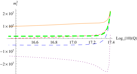
Figure 1: Evolution of soft masses from Planck scale to GUT scale. Dashed (red), dotted (purple), medium dashed (blue), thick dashed (green) and solid (orange) lines represent ${m}^{2}_{\bar{\Phi}}$, ${m}^{2}_{H}$, ${m}^{2}_{\Theta}$, ${m}^{2}_{\Sigma}$ and ${m}^{2}_{\bar{\Sigma}}$ respectively.

$$\begin{array}[]{ccc}\hline\cr\hline\cr&&\vspace{-.3 cm}\hfil\\ {\rm Parameter}&\mbox{Value at $M_{E}=10^{17.4}$ GeV}&\mbox{Value at $M_{X}^{0}(10^{16.33})$ GeV}\vspace{0.1 cm}\\ \hline\cr\hline\cr&&\vspace{-.4 cm}\hfil\\ \tilde{\lambda},\tilde{\eta}&-434.0+78.0i,-3127.0+798.0i&-17.47+3.14i,-335.8+85.69i\\ \tilde{\rho},\tilde{k}&954.4-269.8i,273.0+991i&-115.7+32.7i,-6.39-23.19i\\ \tilde{\gamma},\tilde{\bar{\gamma}}&4711+0.0i,-32719+0.0i&-80.3+0.116i,142.7+0.021i\\ \tilde{\zeta},\tilde{\bar{\zeta}}&10091+8305i,3596+5898i&125.28+103.1i,206.77+339.14i\\ \hline\cr\hline\cr&&\vspace{-.4 cm}\hfil\\ \tilde{h}_{11}/10^{-4}&446.02&63.05+0.0028i\\ \tilde{h}_{22},\tilde{h}_{33}&4.10,244.19&0.58+2.647\times 10^{-5}i,34.52+0.00158i\\ \tilde{h}_{12}/10^{-8},\tilde{h}_{13}/10^{-7}&0.0,0.0&-3.65+5.88i,-3.071+4.62i\\ \tilde{h}_{23}/10^{-5}&0.0&-7.072+13.2i\\ \tilde{f}_{11}/10^{-3},\tilde{f}_{22}&-0.0436+1.621i,.667+0.4845i&-0.042+1.58i,0.65+0.472i\\ \tilde{f}_{33},\tilde{f}_{12}/10^{-2}&-9.264+2.787i,-0.85-1.78i&-9.013+2.71i,-0.83-1.73i\\ \tilde{f}_{13}/10^{-2},\tilde{f}_{23}&0.55+1.15i,-0.427+2.23i&0.535+1.12i,-0.415+2.17i\\ \tilde{g}_{12}&0.146+0.16i&0.073+0.08i\\ \tilde{g}_{13},\tilde{g}_{23}&-1.178+0.496i,-1.665-1.184i&-0.591+0.249i,-0.835-.594i\\ \hline\cr\hline\cr&&\vspace{-.7 cm}\hfil\\ {M_{\tilde{g}}}&0&-1171.73+0.0016i\\ \hline\cr\hline\cr&&\vspace{-.7 cm}\hfil\\ {b_{\Phi}}&5.0\times 10^{18}\mbox{GeV}^{2}&-3.605\times 10^{17}+6.576\times 10^{12}i\mbox{GeV}^{2}\\ {b}_{H}&5.0\times 10^{18}\mbox{GeV}^{2}&-3.579\times 10^{17}+2.474\times 10^{13}i\mbox{GeV}^{2}\\ {b}_{\Sigma}&5.0\times 10^{18}\mbox{GeV}^{2}&3.881\times 10^{17}+6.82\times 10^{12}i\mbox{GeV}^{2}\\ {b}_{\Theta}&5.0\times 10^{18}\mbox{GeV}^{2}&-8.72\times 10^{17}-8.536\times 10^{11}i\mbox{GeV}^{2}\\ \hline\cr\hline\cr&&\vspace{-.4 cm}\hfil\\ {m}^{2}_{\Phi}&2.5\times 10^{7}\mbox{GeV}^{2}&48070.7\mbox{GeV}^{2}\\ {m}^{2}_{H}&2.5\times 10^{7}\mbox{GeV}^{2}&-1.388\times 10^{7}\mbox{GeV}^{2}\\ {m}^{2}_{\Theta}&2.5\times 10^{7}\mbox{GeV}^{2}&-5.154\times 10^{6}\mbox{GeV}^{2}\\ {m}^{2}_{\Sigma}&2.5\times 10^{7}\mbox{GeV}^{2}&1.80955\times 10^{6}\mbox{GeV}^{2}\\ {m}^{2}_{\bar{\Sigma}}&2.5\times 10^{7}\mbox{GeV}^{2}&9.564\times 10^{6}\mbox{GeV}^{2}\vspace{0.1 cm}\\ {\rm Eval~{}{m}^{2}_{\tilde{\Psi}}}&2.5\times 10^{7}\mbox{GeV}^{2}&\{2.7892,2.7892,2.7889\}\times 10^{7}\mbox{GeV}^{2}\vspace{0.1 cm}\\ \hline\cr\hline\cr\end{array}$$

Table 4: Values of NMSGUT soft parameters at two different scales evolved by using one-loop SO(10) RGEs. $A_{0}=10$ TeV, $m_{3/2}=5$ TeV.

IV Concerning Invariant parameter submanifolds under the MSGUT RG flow

The seminal work of Pendleton and Rosspendlross on quasi fixed points of the SM RG flow successfully estimated the approximate top quark mass before its discovery on the basis of the intuition of an approximate “quasi infra red fixed point” in the RG flow governing the ratio $h_{t}^{2}/\alpha_{s}$. Since then the same basic idea has been applied to the dimensionless and even dimensionful(i.e. soft) parameters of (Susy) GUTs to study lanzagross whether the quasi-fixed point structure of the GUT Yukawa and gauge couplings may be significant in fixing the couplings at the Unification scale. It was found that such structures are particularly relevant in the case where there are many fields so that the GUT model is strongly coupled in the ultraviolet. This is precisely the case for the MSGUT and NMSGUT. If such invariant structures could be identified they would obviously be an important criterion for comparing different unified models. In the present instance we have calculated the full set of RG equations for both hard and soft couplings of the MSGUT. Thus the optimistic view might be that these complex flow equations somehow support novel invariant structures when considered in their entirety. The generic form of the 1 loop beta functions for the dimensionless (gauge and Yukawa ) couplings of a supersymmetric model is

$$\beta_{g}= = {\frac{1}{16\pi^{2}}}b_{0}g^{3}$$

$$\beta_{Y^{ijk}} = {\frac{1}{16\pi^{2}}}(\gamma_{i}+\gamma_{j}+\gamma_{k})Y^{ijk}$$ (38)

where $\gamma_{i}$ is given by eqn(9) after using diagonality ( $\gamma^{i}_{j}\equiv\gamma_{i}\delta^{i}_{j}$) of the anomalous dimension matrices , and $b_{0}$ is a large integer or rational number ($b_{0}=137$ for the MSGUT ). It is clear that combining these two equations and the 1-loop formula for $\gamma_{i}$ we can derive fixed point conditions in terms of $Z_{ijk}=|Y_{ijk}|^{2}/g^{2}$ for the squared magnitudes of various couplings , while their phases remain free. These conditions are readily seen to be generically of the form

$$\gamma_{i}+\gamma_{j}+\gamma_{k}-b_{0}g^{2}=0={\frac{\bar{\gamma}_{i}+\bar{\gamma}_{j}+\bar{\gamma}_{k}}{g^{2}}}-(b_{ijk}+b_{0})$$ (39)

where we have separated out the gauge ($b_{ijk}$)and Yukawa($\bar{\gamma}_{i,j,k}$) components of the anomalous dimensions for fields i,j,k. Writing $\bar{\gamma}_{i}=a_{i}^{I}|Y_{I}|^{2}$ where $I$ runs over the different Yukawa couplings in the theory we get the fixed point conditions in the form

$$(a_{i}^{I}+a_{j}^{I}+a_{k}^{I})Z_{I}-(b_{ijk}+b_{0})=0$$ (40)

where $Z_{I}=|Y_{I}|^{2}/g^{2}$.

The question as to whether any quasi fixed points of the full set of RG equations can possibly exist then involves solving these equations subject to the constraints that all $Z_{I}$ are positive semi-definite. Unfortunately the huge value of the coefficient $b_{0}$ which is common to all the conditions makes a solution impossible to achieve.

We illustrate the difficulty for a simplified MSGUT model with negligible first generation matter Yukawas $(h,f,g)_{1A}\simeq 0$,diagonal $h,f$ couplings $h_{2,3},f_{2,3}$ and $g_{32}=-g_{23}$. The relevant anomalous dimensions are

$${\frac{\bar{\gamma}_{\Phi}}{g^{2}}} = 4Z_{k}+180Z_{\lambda}+2Z_{\rho}+240Z_{\eta}+6(Z_{\gamma}+Z_{\bar{\gamma}})+60(Z_{\zeta}+Z_{\bar{\zeta}})$$

$${\frac{\bar{\gamma}_{\bar{\Sigma}}}{g^{2}}} = 200Z_{\eta}+10Z_{\bar{\gamma}}+100Z_{\bar{\zeta}}+32(Z_{f_{2}}+Z_{f_{3}})$$

$${\frac{\bar{\gamma}_{\Sigma}}{g^{2}}} = 200Z_{\eta}+10Z_{\gamma}+100Z_{\zeta}$$

$${\frac{\bar{\gamma}_{H}}{g^{2}}} = 84Z_{k}+126(Z_{\gamma}+Z_{\bar{\gamma}})+8(Z_{h_{2}}+Z_{h_{3}})$$

$${\frac{\bar{\gamma}_{\Theta}}{g^{2}}} = 7Z_{k}+7Z_{\rho}+105(Z_{\zeta}+Z_{\bar{\zeta}})+16Z_{g_{23}}$$

$${\frac{\bar{\gamma}_{\psi}^{T}}{g^{2}}} = 252(0,Z_{f_{2}},Z_{f_{3}})+120(0,Z_{g_{23}},Z_{g_{23}})+10(0,Z_{h_{2}},Z_{h_{3}})$$ (41)

Consider first the case where the couplings to the 16-plets have been set to zero($Z_{h_{2,3},f_{2,3},g_{23}}\equiv 0$). The fixed point conditions for the other couplings are then

$$0 = 3{\frac{\bar{\gamma}_{\Phi}}{g^{2}}}-(b_{0}+72)$$

$$0 = {\frac{(\bar{\gamma}_{\Phi}+\bar{\gamma}_{\Sigma}+\bar{\gamma}_{H})}{g^{2}}}-(b_{0}+58)$$

$$0 = {\frac{(\bar{\gamma}_{\Phi}+{\bar{\gamma}}_{\bar{\Sigma}}+{\bar{\gamma}_{H}})}{g^{2}}}-(b_{0}+58)$$

$$0 = {\frac{(\bar{\gamma}_{\Phi}+\bar{\gamma}_{\Sigma}+\bar{\gamma}_{\bar{\Sigma}})}{g^{2}}}-(b_{0}+74)$$

$$0 = {\frac{(\bar{\gamma}_{\Theta}+\bar{\gamma}_{H}+\bar{\gamma}_{\Phi})}{g^{2}}}-(b_{0}+54)$$

$$0 = {\frac{(2\bar{\gamma}_{\Theta}+\bar{\gamma}_{\Phi})}{g^{2}}}-(b_{0}+66)$$

$$0 = {\frac{(\bar{\gamma}_{\Phi}+\bar{\gamma}_{\Sigma}+\bar{\gamma}_{\Theta})}{g^{2}}}-(b_{0}+70)$$

$$0 = {\frac{(\bar{\gamma}_{\Phi}+\bar{\gamma}_{\Theta}+\bar{\gamma}_{\bar{\Sigma}})}{g^{2}}}-(b_{0}+70)$$ (42)

Solving these fixes $Z_{\eta,k,\zeta,\bar{\zeta},\rho}$ in terms of $Z_{\lambda,\gamma,\bar{\gamma}}$ and for them to be semipositive gives 5 inequalities which can be easily reduced by eliminating $Z_{\gamma}$ between them. However this yields the condition $Z_{\lambda}\leq-227/2700$ which is inconsistent with the semipositive values allowed for $Z_{\lambda}$. So there is no fixed point.

One might hope that introducing the 16-plet couplings might help. Then we restore $Z_{h_{2,3},f_{2,3},g_{23}}$ and obtain the additional conditions for the beta functions of these ratios :

$$0 = {\frac{(\bar{\gamma}_{H}+2\bar{\gamma}_{\psi_{2,3}})}{g^{2}}}-(b_{0}+63/2)$$

$$0 = {\frac{(\bar{\gamma}_{\bar{\Sigma}}+2\bar{\gamma}_{\psi_{2,3}})}{g^{2}}}-(b_{0}+95/2)$$

$$0 = {\frac{(\bar{\gamma}_{\Theta}+\bar{\gamma}_{\psi_{2}}+\bar{\gamma}_{\psi_{3}})}{g^{2}}}-(b_{0}+87/2)$$ (43)

Solving these conditions one finds that $Z_{\zeta,\bar{\zeta},h_{3},f_{2},f_{3},g_{23},\rho}$ are determined in terms of $Z_{\eta,\gamma,\bar{\gamma},k,\lambda,h_{2}}\geq 0$ which are themselves undetermined. The question is whether there are any semipositive values of these free parameters for which the dependent variables remain semipositive. Solution of the fixed point conditions yields the following solution vector

$$\{Z_{\zeta},Z_{\bar{\zeta}},Z_{h_{3}},Z_{f_{2}},Z_{f_{3}},Z_{g_{23}},Z_{\rho}\}=$$

$$\{53/75-2Z_{\eta}-Z_{\gamma}/10,689/525-10Z_{\eta}-Z_{\bar{\gamma}}/10-12Z_{\lambda},$$

$$41/6-(63Z_{\gamma})/4-(63Z_{\bar{\gamma}})/4-Z_{h_{2}}-(21Z_{k})/2,$$

$$-(613/756)+(25Z_{\eta})/2-(5Z_{\gamma})/16-(5Z_{\bar{\gamma}})/16-(5Z_{h_{2}})/126-5Z_{k}/24+(75Z_{\lambda})/4,$$

$$-(409/378)+(25Z_{\eta})/2+(5Z_{\gamma})/16+(5Z_{\bar{\gamma}})/16+(5Z_{h_{2}})/126+(5Z_{k})/24+(75Z_{\lambda})/4,$$

$$209/96-(105Z_{\eta})/4+(21Z_{\gamma})/32+(21Z_{\bar{\gamma}})/32+(7Z_{k})/16-(315Z_{\lambda})/8,$$

$$-(1081/42)+240Z_{\eta}-(2Z_{k})+270Z_{\lambda}\}\geq 0$$ (44)

An elementary reduction of this system of inequalities solod leads to contradictory condition

$$-(407+252Z_{k}+11340Z_{\lambda})/48\geq Z_{h_{2}}\geq 0$$ (45)

showing that again there is no fixed point for the system even when measuring in units of the (exploding in the UV) value of $g^{2}$. Although we have not obtained a general proof it seems likely that no fixed point can be found. Support for this can be found in recent investigations bajcsann , based on the so called non-perturbative a-theorem and the exact NSVZ beta function(see bajcsann for a concise introduction and a fairly complete list of references for these topics), of the possibility of non-trivial superconformal UV fixed points in the SO(10) MSGUT. They conclude that no such fixed points exist without rather artificial requirements being placed upon the couplings and R-charges of some of the SO(10) multiplets or by introducing very large numbers of additional multiplets and trivializing the superpotentials allowed.

V Discussion

We have proposed a framework for a consistent interpretation of Asymptotically Strong GUTs by considering RG flows of GUT parameters from an emergence scale $M_{E}$ of a weakly coupled GUT down to the scale $M_{X}$ where the GUT is matched to its low energy effective theory. Thereafter the MSSM flows from $M_{X}$ down to $M_{Z}$ determine the experimental predictions of the GUT parameter set chosen at $M_{E}$. This procedure allows extension of the perturbative regime of the unified theory up to the Landau Polar latitude $\Lambda_{E}$. Interestingly the large number of degrees of freedom further strengthen the intuitiontrmin ; tas that the scale of Gravity may be dominantly set by the effects of (the thousands of) NMSGUT superheavy particles. Thus $M_{Pl}$ can lie well above $\Lambda_{E}$ which nevertheless plays a part in raising $M_{Pl}$ by serving as the physical cutoff scale for graviton wave function renormalization corrections due to the NMSGUT as well as the scale for SO(10) “confinement” tas . We presented the NMSGUT RG equations to determine the RG evolution of couplings between the scale($M_{E}$) where the perturbative effective theory (NMSGUT plus weakly coupled and softly broken $N=1$ supergravity) emerges and the matching scale between GUT and the low energy effective theory (i.e the MSSM) at $M_{X}$. To illustrate the application of these results we evaluated the effects of the 1-loop evolution on randomly chosen sets of parameter values assuming a minimal, canonical kinetic term, supergravity scenario for the starting parameter ansatz. From the Tables and Fig. 1 we see that the RG evolution has dramatic effects on the soft Susy breaking parameters. Firstly most of the soft Susy breaking Hermitian masses squared of the SO(10) Higgs irreps become negative even though they start from a common positive mass. This provides a potentially robust justification of the negative values of $M_{H,\bar{H}}^{2}$ used in NMSGUT fits nmsgut ; bstabhedge . Note that the distinctive normal s-hierarchy at low scale is strongly correlated with the large negative $M_{H,\bar{H}}^{2}$ we use in the fits. Gaugino masses($M_{\lambda}$) will be generated by two loop RG evolution between $M_{X}$ and $M_{Z}$, even if $M_{\lambda}$=0 at the scale $M_{X}$. On the other hand the same applies to the evolution between $M_{E}$ and $M_{X}$. Thus even canonical gauge kinetic terms in the GUT can still generate adequate gaugino masses. This is pleasing since we have always resisted invoking non canonical K$\ddot{a}$hler potential and gauge kinetic terms on grounds of minimality/predictivity and to preserve renormalizability of the gauge sector.

Another notable effect is the intermediate scale $(O({m_{3/2}M_{X}}))$ values of the soft parameters $b_{\Phi,\Sigma,\Theta,H}$ required by the canonical mSUGRY ansatz and induced by the dependence $\frac{db}{dt}$ $\sim$ $M_{X}m_{3/2}$. So we may need to impose an additional condition in order that the contribution from the soft terms to $b_{H,\bar{H}}$ is O($m_{3/2}^{2}$) unless this is achievable via the RG flow of $B_{ij}$ towards negative values itself.

The running of trilinear soft coupling and s-fermion mass squared parameters ($m_{\tilde{\Psi}}^{2}$) will give distinct values at the GUT scale for the three generations (considered the same in earlier studies of NMSGUTnmsgut ; bstabhedge ). In sequels we will integrate these RG flows with our previous code that incorporates the MSSM flows between $M_{X}$ and $M_{Z}$. Then one will throw the core soft parameters $m_{3/2},A_{0}$ at $M_{E}$ and run down over thresholds to $M_{Z}$ with one additional fine tuning constraint. Thus the total number of soft parameters will be significantly reduced. Improvements would include the 2-loop RG coefficients we have already computed phds . Finally the straightforward (since the superpotential vertex connectivity is preserved) generalization of these results to the case of YUMGUTsyumgut will allow us also to perform the RG flows from the Planck scale for dynamical flavour generation models based on the MSGUT. These theories have around 6 times as many fields as the NMSGUT and are thus even more capable of separating $M_{X}$ and $M_{Pl}$. We note that the techniques we have used to actually evaluate the 2-loop RGEs have overcome the combinatorial complexity that prevented their calculation by automated means. They can be used for any Susy GUT.

VI Acknowledgements

CSA acknowledges financial support from the the Department of Science and Technology, Government of India , under SERB Project No. EMR/2014/000250 on the “ Phenomenology and Cosmology of the New Minimal Supersymmetric SO(10) GUT”.

Appendix

One-loop RGEs

One-loop anomalous dimension parameters associated with different superfields:

$$\gamma_{i}^{(1)j} = \frac{1}{2}Y_{ipq}Y^{jpq}-2g_{10}^{2}\delta_{i}^{j}C(i)$$

$$\gamma_{\Sigma}^{(1)} = 200|\eta|^{2}+10|\gamma|^{2}+100|\zeta|^{2}-25g_{10}^{2}$$

$$\gamma_{\bar{\Sigma}}^{(1)} = 200|\eta|^{2}+10|\bar{\gamma}|^{2}+100|\bar{\zeta}|^{2}+32\text{Tr}[f^{{\dagger}}.f]-25g_{10}^{2}$$

$$\gamma_{H}^{(1)} = 84|\kappa|^{2}+126(|\gamma|^{2}+|\bar{\gamma}|^{2})+8\text{Tr}[h^{{\dagger}}.h]-9g_{10}^{2}$$

$$\gamma_{\Theta}^{(1)} = 7(|\kappa|^{2}+|\rho|^{2})+105(|\zeta|^{2}+|\bar{\zeta}|^{2})+8\text{Tr}[g^{{\dagger}}.g]-21g_{10}^{2}$$

$$(\gamma_{\Psi}^{(1)})_{A}^{B} = (\gamma_{\Psi}^{(1)})_{AB}=252f^{{\dagger}}.f+120g^{{\dagger}}.g+10h^{{\dagger}}.h-\frac{45g_{10}^{2}}{4}$$ (46)

$$\bar{\gamma}_{i}^{(1)j} = \frac{1}{2}Y_{ipq}Y^{jpq}$$

$$\bar{\gamma}_{\Sigma}^{(1)} = 200|\eta|^{2}+10|\gamma|^{2}+100|\zeta|^{2}$$

$$\bar{\gamma}_{\bar{\Sigma}}^{(1)} = 200|\eta|^{2}+10|\bar{\gamma}|^{2}+100|\bar{\zeta}|^{2}+32\text{Tr}[f^{{\dagger}}.f]$$

$$\bar{\gamma}_{H}^{(1)} = 84|\kappa|^{2}+126(|\gamma|^{2}+|\bar{\gamma}|^{2})+8\text{Tr}[h^{{\dagger}}.h]$$

$$\bar{\gamma}_{\Theta}^{(1)} = 7(|\kappa|^{2}+|\rho|^{2})+105(|\zeta|^{2}+|\bar{\zeta}|^{2})+8\text{Tr}[g^{{\dagger}}.g]$$

$$\bar{\gamma}_{\Psi}^{(1)} = 252f^{{\dagger}}.f+120g^{{\dagger}}.g+10h^{{\dagger}}.h$$ (47)

One-loop beta functions for the SO(10) superpotential parameters and Yukawa couplings are:

$$\beta_{\lambda}^{(1)}=3\gamma_{\Phi}^{(1)}\lambda\quad;\quad\beta_{\eta}^{(1)}=\eta(\gamma_{\Sigma}^{(1)}+\gamma_{\bar{\Sigma}}^{(1)}+\gamma_{\Phi}^{(1)})$$ (48)

$$\beta_{\gamma}^{(1)}=\gamma(\gamma_{H}^{(1)}+\gamma_{\Sigma}^{(1)}+\gamma_{\Phi}^{(1)})\quad;\quad\beta_{\bar{\gamma}}^{(1)}=\bar{\gamma}(\gamma_{H}^{(1)}+\gamma_{\bar{\Sigma}}^{(1)}+\gamma_{\Phi}^{(1)})$$ (49)

$$\beta_{k}^{(1)}=k(\gamma_{H}^{(1)}+\gamma_{\Theta}^{(1)}+\gamma_{\Phi}^{(1)})\quad;\quad\beta_{\zeta}^{(1)}=\zeta(\gamma_{\Theta}^{(1)}+\gamma_{\Sigma}^{(1)}+\gamma_{\Phi}^{(1)})$$ (50)

$$\beta_{\bar{\zeta}}^{(1)}=\bar{\zeta}(\gamma_{\Theta}^{(1)}+\gamma_{\bar{\Sigma}}^{(1)}+\gamma_{\Phi}^{(1)})\quad;\quad\beta_{\rho}^{(1)}=\rho(\gamma_{\Phi}^{(1)}+2\gamma_{\Theta}^{(1)})$$ (51)

$$\beta_{h}^{(1)}=h\gamma_{H}^{(1)}+(\gamma_{\Psi}^{(1)})^{T}.h+h.\gamma_{\Psi}^{(1)}\quad;\quad\beta_{f}^{(1)}=f\gamma_{\bar{\Sigma}}^{(1)}+(\gamma_{\Psi}^{(1)})^{T}.f+f.\gamma_{\Psi}^{(1)}$$ (52)

$$\beta_{g}^{(1)}=g\gamma_{\Theta}^{(1)}-(\gamma_{\Psi}^{(1)})^{T}.g+g.\gamma_{\Psi}^{(1)}$$ (53)

$$\beta_{\mu_{\Phi}}^{(1)}=2\gamma_{\Phi}^{(1)}\mu_{\Phi}\quad;\quad\beta_{\mu_{H}}^{(1)}=2\gamma_{H}^{(1)}\mu_{H}$$ (54)

$$\beta_{\mu_{\Sigma}}^{(1)}=(\gamma_{\Sigma}^{(1)}+\gamma_{\bar{\Sigma}}^{(1)})\mu_{\Sigma}\quad;\quad\beta_{\mu_{\Theta}}^{(1)}=2\gamma_{\Theta}^{(1)}\mu_{\Theta}$$ (55)

Soft parameters RGEs

$$\tilde{\gamma}_{i}^{(1)j} = \frac{1}{2}Y_{ipq}h^{jpq}$$

$$\tilde{\gamma}_{\Sigma}^{(1)} = 200\tilde{\eta}\eta^{*}+10\tilde{\gamma}\gamma^{*}+100\tilde{\zeta}\zeta^{*}$$

$$\tilde{\gamma}_{\bar{\Sigma}}^{(1)} = 200\tilde{\eta}\eta^{*}+10\tilde{\bar{\gamma}}\bar{\gamma}^{*}+100\tilde{\bar{\zeta}}\bar{\zeta}^{*}+32\text{Tr}[f^{{\dagger}}.\tilde{f}]$$

$$\tilde{\gamma}_{H}^{(1)} = 84\tilde{\kappa}\kappa^{*}+126(\tilde{\gamma}\gamma^{*}+\tilde{\bar{\gamma}}\bar{\gamma}^{*})+8\text{Tr}[h^{{\dagger}}.\tilde{h}]$$

$$\tilde{\gamma}_{\Theta}^{(1)} = 7(\tilde{\kappa}\kappa^{*}+\tilde{\rho}\rho^{*})+105(\tilde{\zeta}\zeta^{*}+{\tilde{\bar{\zeta}}}\bar{\zeta}^{*})+8\text{Tr}[g^{{\dagger}}.\tilde{g}]$$

$$\tilde{\gamma}_{\psi}^{(1)} = 252f^{{\dagger}}.\tilde{f}+120g^{{\dagger}}.\tilde{g}+10h^{{\dagger}}.\tilde{h}$$ (56)

$$\hat{\gamma}_{i}^{(1)j} = \frac{1}{2}h_{ipq}h^{jpq}$$

$$\hat{\gamma}_{\Phi}^{(1)} = 240|\tilde{\eta}|^{2}+4|\tilde{\kappa}|^{2}+180|\tilde{\lambda}|^{2}+2|\tilde{\rho}|^{2}+6(|\tilde{\gamma}|^{2}+|\tilde{\bar{\gamma}}|^{2})+60(|\tilde{\zeta}|^{2}+|\tilde{\bar{\zeta}}|^{2})$$

$$\hat{\gamma}_{\Sigma}^{(1)} = 200|\tilde{\eta}|^{2}+10|\tilde{\gamma}|^{2}+100|\tilde{\zeta}|^{2}$$

$$\hat{\gamma}_{\bar{\Sigma}}^{(1)} = 200|\tilde{\eta}|^{2}+10|\tilde{\bar{\gamma}}|^{2}+100|\tilde{\bar{\zeta}}|^{2}+32\text{T}r[\tilde{f}^{{\dagger}}.\tilde{f}]$$

$$\hat{\gamma}_{H}^{(1)} = 84|\tilde{\kappa}|^{2}+126(|\tilde{\gamma}|^{2}+|\tilde{\bar{\gamma}}|^{2})+8\text{T}r[\tilde{h}^{{\dagger}}.\tilde{h}]$$

$$\hat{\gamma}_{\Theta}^{(1)} = 7(|\tilde{\kappa}|^{2}+|\tilde{\rho}|^{2})+105(|\tilde{\zeta}|^{2}+|\tilde{\bar{\zeta}}|^{2})+8\text{T}r[\tilde{g}^{{\dagger}}.\tilde{g}]$$

$$\hat{\gamma}_{\Psi}^{(1)} = 252\tilde{f}^{{\dagger}}.\tilde{f}+120\tilde{g}^{{\dagger}}.\tilde{g}+10\tilde{h}^{{\dagger}}.\tilde{h}$$ (57)

One-loop beta functions for the soft parameters:

$$\beta_{\tilde{\eta}}^{(1)}=\tilde{\eta}(\bar{\gamma}_{\Phi}^{(1)}+\bar{\gamma}_{\Sigma}^{(1)}+\bar{\gamma}_{\bar{\Sigma}}^{(1)})+2\eta(\tilde{\gamma}_{\Phi}^{(1)}+\tilde{\gamma}_{\Sigma}^{(1)}+\tilde{\gamma}_{\bar{\Sigma}}^{(1)})-74g_{10}^{2}(\tilde{\eta}-2M\eta)$$ (58)

$$\beta_{\tilde{\gamma}}^{(1)}=\tilde{\gamma}(\bar{\gamma}_{\Phi}^{(1)}+\bar{\gamma}_{\Sigma}^{(1)}+\bar{\gamma}_{H}^{(1)})+2\gamma(\tilde{\gamma}_{\Phi}^{(1)}+\tilde{\gamma}_{\Sigma}^{(1)}+\tilde{\gamma}_{H}^{(1)})-58g_{10}^{2}(\tilde{\gamma}-2M\gamma)$$ (59)

$$\beta_{\tilde{\bar{\gamma}}}^{(1)}=\tilde{\bar{\gamma}}(\bar{\gamma}_{\Phi}^{(1)}+\bar{\gamma}_{\bar{\Sigma}}^{(1)}+\bar{\gamma}_{H}^{(1)})+2\bar{\gamma}(\tilde{\gamma}_{\Phi}^{(1)}+\tilde{\gamma}_{\bar{\Sigma}}^{(1)}+\tilde{\gamma}_{H}^{(1)})-58g_{10}^{2}(\tilde{\bar{\gamma}}-2M\bar{\gamma})$$ (60)

$$\beta_{\tilde{\kappa}}^{(1)}=\tilde{\kappa}(\bar{\gamma}_{\Phi}^{(1)}+\bar{\gamma}_{\Theta}^{(1)}+\bar{\gamma}_{H}^{(1)})+2\kappa(\tilde{\gamma}_{\Phi}^{(1)}+\tilde{\gamma}_{\Theta}^{(1)}+\tilde{\gamma}_{H}^{(1)})-54g_{10}^{2}(\tilde{\kappa}-2M\kappa)$$ (61)

$$\beta_{\tilde{\rho}}^{(1)}=\tilde{\rho}(\bar{\gamma}_{\Phi}^{(1)}+2\bar{\gamma}_{\Theta}^{(1)})+2\rho(\tilde{\gamma}_{\Phi}^{(1)}+2\tilde{\gamma}_{\Theta}^{(1)})-66g_{10}^{2}(\tilde{\rho}-2M\rho)$$ (62)

$$\beta_{\tilde{\zeta}}^{(1)}=\tilde{\zeta}(\bar{\gamma}_{\Phi}^{(1)}+\bar{\gamma}_{\Sigma}^{(1)}+\bar{\gamma}_{\Theta}^{(1)})+2\zeta(\tilde{\gamma}_{\Phi}^{(1)}+\tilde{\gamma}_{\Sigma}^{(1)}+\tilde{\gamma}_{\Theta}^{(1)})-70g_{10}^{2}(\tilde{\zeta}-2M\zeta)$$ (63)

$$\beta_{\tilde{\bar{\zeta}}}^{(1)}=\tilde{\bar{\zeta}}(\bar{\gamma}_{\Phi}^{(1)}+\bar{\gamma}_{\bar{\Sigma}}^{(1)}+\bar{\gamma}_{\Theta}^{(1)})+2\bar{\zeta}(\tilde{\gamma}_{\Phi}^{(1)}+\tilde{\gamma}_{\bar{\Sigma}}^{(1)}+\tilde{\gamma}_{\Theta}^{(1)})-70g_{10}^{2}(\tilde{\bar{\zeta}}-2M\bar{\zeta})$$ (64)

$$\beta_{\tilde{h}}^{(1)}=\bar{\gamma}_{H}^{(1)}\tilde{h}+\tilde{h}.\bar{\gamma}_{\Psi}^{(1)}+(\bar{\gamma}_{\Psi}^{(1)})^{T}.\tilde{h}+2\tilde{\gamma}_{H}^{(1)}h+2(h.\tilde{\gamma}_{\Psi}^{(1)}+(\tilde{\gamma}_{\Psi}^{(1)})^{T}.h)-\frac{63}{2}g_{10}^{2}(\tilde{h}-2Mh)$$ (65)

$$\beta_{\tilde{g}}^{(1)}=\bar{\gamma}_{\Theta}^{(1)}\tilde{g}-\tilde{g}.\bar{\gamma}_{\Psi}^{(1)}+(\bar{\gamma}_{\Psi}^{(1)})^{T}.\tilde{g}+2\tilde{\gamma}_{\Theta}^{(1)}.g+2(g.\tilde{\gamma}_{\Psi}^{(1)}-(\tilde{\gamma}_{\Psi}^{(1)})^{T}.g)-\frac{87}{2}g_{10}^{2}(\tilde{g}-2Mg)$$ (66)

$$\beta_{\tilde{f}}^{(1)}=\bar{\gamma}_{\bar{\Sigma}}^{(1)}\tilde{f}+\tilde{f}.\bar{\gamma}_{\Psi}^{(1)}+(\bar{\gamma}_{\Psi}^{(1)})^{T}.\tilde{f}+2\tilde{\gamma}_{\bar{\Sigma}}^{(1)}.f+2(f.\tilde{\gamma}_{\Psi}^{(1)}+(\tilde{\gamma}_{\Psi}^{(1)})^{T}.f)-\frac{95}{2}g_{10}^{2}(\tilde{f}-2Mf)$$ (67)

$$\beta_{b_{\Phi}}^{(1)}=2b_{\Phi}\bar{\gamma}_{\Phi}^{(1)}+4\mu_{\Phi}\tilde{\gamma}_{\Phi}^{(1)}-48g_{10}^{2}(b_{\Phi}-2M\mu_{\Phi})$$ (68)

$$\beta_{b_{H}}^{(1)}=2b_{H}\bar{\gamma}_{H}^{(1)}+4\mu_{H}\tilde{\gamma}_{H}^{(1)}-18g_{10}^{2}(b_{H}-2M\mu_{H})$$ (69)

$$\beta_{b_{\Theta}}^{(1)}=2b_{\Theta}\bar{\gamma}_{\Theta}^{(1)}+4\mu_{\Theta}\tilde{\gamma}_{\Theta}^{(1)}-42g_{10}^{2}(b_{\Theta}-2M\mu_{\Theta})$$ (70)

$$\beta_{b_{\Sigma}}^{(1)}=b_{\Sigma}(\bar{\gamma}_{\Sigma}^{(1)}+\bar{\gamma}_{\bar{\Sigma}}^{(1)})+2\mu_{\Sigma}(\tilde{\gamma}_{\Sigma}^{(1)}+\tilde{\gamma}_{\bar{\Sigma}}^{(1)})-50g_{10}^{2}(b_{\Sigma}-2M\mu_{\Sigma})$$ (71)

$$\beta_{m^{2}_{\Phi}}^{(1)} = 2\bar{\gamma}_{\Phi}^{(1)}m^{2}_{\Phi}+720m^{2}_{\Phi}|\lambda|^{2}+m^{2}_{H}(12|\gamma|^{2}+12|\bar{\gamma}|^{2}+8|\kappa|^{2})$$ (72)

$$+m^{2}_{\Theta}(8|\rho|^{2}+120(|\zeta|^{2}+|\bar{\zeta}|^{2})+8|\kappa|^{2})+m^{2}_{\Sigma}(480|\eta|^{2}+12|\gamma|^{2}+120|\zeta|^{2})$$

$$+m^{2}_{\bar{\Sigma}}(480|\eta|^{2}+12|\bar{\gamma}|^{2}+120|\bar{\zeta}|^{2})+2\hat{\gamma}_{\Phi}^{(1)}-96|M|^{2}g_{10}^{2}$$

$$\beta_{m^{2}_{H}}^{(1)} = 2\bar{\gamma}_{H}^{(1)}m^{2}_{H}+m^{2}_{\Phi}(252(|\gamma|^{2}+|\bar{\gamma}|^{2})+168|\kappa|^{2})+168m^{2}_{\Theta}|\kappa|^{2}+252m^{2}_{\Sigma}|\gamma|^{2}$$ (73)

$$+252m^{2}_{\bar{\Sigma}}|\bar{\gamma}|^{2}+2\hat{\gamma}_{H}^{(1)}-36|M|^{2}g_{10}^{2}+32\text{T}r[h^{{\dagger}}.m^{2}_{\tilde{\Psi}}.h]$$

$$\beta_{m^{2}_{\Theta}}^{(1)} = 2\bar{\gamma}_{\Theta}^{(1)}m^{2}_{\Theta}+m^{2}_{\Phi}(14(|\kappa|^{2}+|\rho|^{2})+210(|\zeta|^{2}+|\bar{\zeta}|^{2}))+14m^{2}_{\Theta}|\rho|^{2}+14m^{2}_{H}|\kappa|^{2}$$ (74)

$$+210m^{2}_{\Sigma}|\zeta|^{2}+210m^{2}_{\bar{\Sigma}}|\bar{\zeta}|^{2}+2\hat{\gamma}_{\Theta}^{(1)}-84|M|^{2}g_{10}^{2}+32\text{T}r[g^{{\dagger}}.m^{2}_{\tilde{\Psi}}.g]$$

$$\beta_{m^{2}_{\Sigma}}^{(1)} = 2\bar{\gamma}_{\Sigma}^{(1)}m^{2}_{\Sigma}+m^{2}_{\Phi}(400|\eta|^{2}+20|\gamma|^{2}+200|\zeta|^{2})+200m^{2}_{\Theta}|\zeta|^{2}+20m^{2}_{H}|\gamma|^{2}$$ (75)

$$+400m^{2}_{\bar{\Sigma}}|\eta|^{2}+2\hat{\gamma}_{\Sigma}^{(1)}-100|M|^{2}g_{10}^{2}$$

$$\beta_{m^{2}_{\bar{\Sigma}}}^{(1)} = 2\bar{\gamma}_{\bar{\Sigma}}^{(1)}m^{2}_{\bar{\Sigma}}+m^{2}_{\Phi}(400|\eta|^{2}+20|\bar{\gamma}|^{2}+200|\bar{\zeta}|^{2})+200m^{2}_{\Theta}|\bar{\zeta}|^{2}+20m^{2}_{H}|\bar{\gamma}|^{2}$$ (76)

$$+400m^{2}_{\Sigma}|\eta|^{2}+2\hat{\gamma}_{\bar{\Sigma}}^{(1)}-100|M|^{2}g^{2}_{10}+128\text{T}r[f^{{\dagger}}.m^{2}_{\tilde{\Psi}}.f]$$

$$\beta_{m^{2}_{\tilde{\Psi}}}^{(1)} = \bar{\gamma}_{\Psi}^{(1)}.m^{2}_{\tilde{\Psi}}+m^{2}_{\tilde{\Psi}}.\bar{\gamma}_{\Psi}^{(1)}+10h^{{\dagger}}.m^{2}_{\tilde{\Psi}}.h+120g^{{\dagger}}.m^{2}_{\tilde{\Psi}}.g+252f^{{\dagger}}.m^{2}_{\tilde{\Psi}}.f+10m^{2}_{H}h^{{\dagger}}.h$$ (77)

$$+120m^{2}_{\Theta}g^{{\dagger}}.g+252m^{2}_{\bar{\Sigma}}f^{{\dagger}}.f+2\hat{\gamma}_{\Psi}^{(1)}-45|M|^{2}g^{2}_{10}$$

References

- (1) J. C. Pati and A. Salam, “Lepton Number as the Fourth Color”, Phys. Rev. D 10, 275 (1974).
- (2) H. Georgi and S. L. Glashow, “Unity Of All Elementary Particle Forces”, Phys. Rev. Lett. 32, 438 (1974).
- (3) H. Georgi, H. R. Quinn and S. Weinberg, Hierarchy of Interactions in Unified Gauge Theories, Phys. Rev. Lett. 33, 451 (1974).
- (4) M. E. Machacek and M. T. Vaughn, Two Loop Renormalization Group Equations in a General Quantum Field Theory. 1. Wave Function Renormalization, Nucl. Phys. B 222, 83 (1983); M. E. Machacek and M. T. Vaughn, Two Loop Renormalization Group Equations in a General Quantum Field Theory. 2. Yukawa Couplings, Nucl. Phys. B 236, 221 (1984); M. E. Machacek and M. T. Vaughn, Two Loop Renormalization Group Equations in a General Quantum Field Theory. 3. Scalar Quartic Couplings, Nucl. Phys. B 249, 70 (1985);
- (5) I. Jack and D. R. T. Jones, Soft supersymmetry breaking and 1091 finiteness, Phys. Lett. B 333 (1994) 372; P. M. Ferreira, I. Jack and D. R. T. Jones, Infra-red soft universality, Phys. Lett. B 357 (1995) 359.
- (6) S. P. Martin and M. T. Vaughn, Two Loop Renormalization Group Equations For Soft Supersymmetry Breaking Couplings, Phys. Rev. D 50, 2282 (1994) [arXiv:hep-ph/9311340]; S. P. Martin, Two-loop effective potential for the minimal supersymmetric standard model, Phys. Rev. D 66, 096001 (2002) [arXiv:hep-ph/0206136].
- (7) I. Jack and D. R. T. Jones, The gaugino -function, Phys. Lett. B 415 (1997) 383, I. Jack and D. R. T. Jones and A. Pickering, The soft scalar mass -function, Phys. Lett. B 432 (1998) 114.
- (8) W. J. Marciano and G. Senjanovic, Predictions of Supersymmetric Grand Unified Theories, Phys. Rev. D 25, 3092 (1982).
- (9) U. Amaldi, W. de Boer and H. Furstenau, Comparison of grand unified theories with electroweak and strong coupling constants measured at LEP, Phys. Lett. B 260 (1991) 447.
- (10) C. S. Aulakh, Truly minimal unification: Asymptotically strong panacea?, hep-ph/0207150.
- (11) C. S. Aulakh, Taming asymptotic strength, hep-ph/0210337.
- (12) G. Dvali, Black Holes and Large N Species Solution to the Hierarchy Problem, Fortsch. Phys. 58 (2010) 528 [arXiv:0706.2050 [hep-th]].
- (13) S.L.Adler, Einstein gravity as a symmetry-breaking effect 1117 in quantum field theory, Rev. Mod. Phys.54(1982)729 and references therein.
- (14) C. S. Aulakh and C. K. Khosa, Grand Yukawonification : SO(10) grand unified theories with dynamical Yukawa couplings, Phys. Rev. D 90, 045008 (2014) [arXiv:1308.5665 [hep-ph]]; C. S. Aulakh, Bajc-Melfo vacua enable Yukawon ultraminimal grand unified theories, Phys. Rev. D 91, 055012 (2015) [arXiv:1402.3979 [hep-ph]].
- (15) F. David, A Comment On Induced Gravity, Phys. Lett. B 138 (1984) 383; F. David and A. Strominger, On the Calculability of Newton’s Constant and the Renormalizability of Scale Invariant Quantum Gravity, Phys. Lett. B 143 (1984) 125.
- (16) C. S. Aulakh and S. K. Garg, The new minimal supersymmetric GUT, [arXiv:hep-ph/0612021v1]; [arXiv:hep-ph/0612021v2]; C. S. Aulakh, Pinning down the new minimal supersymmetric GUT, Phys. Lett. B 661, 196 (2008), [arXiv:0710.3945 [hep-ph]].
- (17) C. S. Aulakh, I. Garg and C. K. Khosa, Baryon Stability on the Higgs Dissolution Edge : Threshold corrections and suppression of Baryon violation in the NMSGUT, Nucl. Phys. B 882, 397 (2014) [arXiv:1311.6100[hep-ph]].
- (18) M.S. Carena, M. Olechowski, S. Pokorski and C. E. M. Wagner, Electroweak symmetry breaking and bottom - top Yukawa unification, Nucl. Phys. B 426, 269 (1994) [arXiv:hep-ph/9402253]. B. Ananthanarayan, Q. Shafi and X. M. Wang, Improved predictions for top quark, lightest supersymmetric particle, and Higgs scalar masses, Phys. Rev. D 50 (1994) 5980 [arXiv:hep-ph/9311225]; R. Rattazzi, U. Sarid and L.J. Hall, Yukawa unification: The good, the bad and the ugly, [arXiv:hep-ph/9405313];
- (19) R. Barbieri, L. J. Hall and A. Strumia, Violations of lepton flavor and CP in supersymmetric unified theories, Nucl. Phys. B 445, 219 (1995) [hep-ph/9501334].
- (20) C.S. Aulakh, NMSGUT-III: Grand Unification upended,[arXiv:hep-ph/1107.2963].
- (21) C.S. Aulakh and R.N. Mohapatra, CCNY-HEP-82-4 April 1982, CCNY-HEP-82-4-REV, Jun 1982 , Implications of supersymmetric SO(10) grand unification, Phys. Rev. D 28, 217 (1983).
- (22) T.E. Clark, T.K. Kuo, and N. Nakagawa, An SO(10) supersymmetric grand unified theory, Phys. lett. B 115, 26(1982).
- (23) R. M. Fonseca, Calculating the renormalisation group equations of a SUSY model with fonseca, Comput. Phys. Commun. 183, 2298 (2012) [arXiv:1106.5016 [hep-ph]].
- (24) J. Wess and B. Zumino, A Lagrangian Model Invariant Under Supergauge Transformations, Phys. Lett. B 49, 52 (1974); J. Iliopoulos and B. Zumino, Broken Supergauge Symmetry and Renormalization, Nucl. Phys. B 76, 310 (1974); S. Ferrara, J. Iliopoulos and B. Zumino, Supergauge Invariance and the Gell-Mann - Low Eigenvalue, Nucl. Phys. B 77, 413 (1974); B. Zumino, Supersymmetry and the Vacuum, Nucl. Phys. B 89, 535 (1975); S. Ferrara and O. Piguet, Perturbation Theory and Renormalization of Supersymmetric Yang-Mills Theories, Nucl. Phys. B 93, 261 (1975); M. T. Grisaru, W. Siegel and M. Rocek, Improved Methods for Supergraphs, Nucl. Phys. B 159, 429 (1979).
- (25) Charanjit Kaur, Study of baryon number and lepton flavour violation in the new minimal supersymmetric SO(10)GUT, arXiv:1506.04101 [hep-ph], Ph.D Thesis, Panjab Uni. Chandigarh, 2014. Ila Garg, New minimal supersymmetric SO(10) GUT phenomenology and its cosmological implications, arXiv:1506.05204 [hep-ph], Ph.D. Thesis, Panjab Uni. Chandigarh, 2014.
- (26) N. Ohta, Grand Unified Theories Based on Local Supersymmetry, Prog. Theor. Phys. 70 (1983) 542; L. J. Hall, J. D. Lykken and S. Weinberg, Supergravity as the Messenger of Supersymmetry Breaking, Phys. Rev. D 27 (1983) 2359. A. H. Chamseddine, R. L. Arnowitt and P. Nath, Locally Supersymmetric Grand Unification, Phys. Rev. Lett. 49 (1982) 970. ; See also R. Arnowitt, A. H. Chamseddine and P. Nath, The Development of Supergravity Grand Unification: Circa 1982-85, Int. J. Mod. Phys. A 27 (2012) 1230028 [Int. J. Mod. Phys. A 27 (2012) 1292009] [arXiv:1206.3175 [physics.hist-ph]]. and citations therein. For a convenient compendium and review of relevant results see : Theory and Phenomenology of Sparticles, by M. Drees, R. Godbole and P. Roy, World Scientific Publishing Co. Pte. Ltd.
- (27) L. Calibbi, D. Chowdhury, A. Masiero, K. M. Patel and S. K. Vempati, Status of supersymmetric type-I seesaw in SO(10) inspired models, JHEP 1211, 040 (2012) [arXiv:1207.7227].
- (28) B. Pendleton and G. G. Ross, Mass and mixing angle 1200 predictions from infra-red fixed points, Phys. Lett. B 98 (1981) 291. C. T. Hill, Phys. Rev. D 24 (1981) 691.
- (29) M. Lanzagorta and G. G. Ross, Quark and lepton masses from 1202 renormalization-group fixed points, Phys. Lett. B 364 (1995) 163; Phys. Lett. B 349 (1995) 319.
- (30) B. Bajc and F. Sannino, Asymptotically Safe Grand Unification, JHEP 1612, 141 (2016), [arXiv:1610.09681 [hep-th]]. An extensive list of references to recent work, particularly by Sannino and collaborators on asymptotically safe Gauge theories is given in this model.
- (31) C. S. Aulakh, K. Benakli and G. Senjanovic, Reconciling supersymmetry and left-right symmetry, Phys. Rev. Lett. 79 (1997) 2188 [hep-ph/9703434]. C. S. Aulakh, A. Melfo and G. Senjanovic, Minimal supersymmetric left-right model, Phys. Rev. D 57 (1998) 4174, [hep-ph/9707256]; C. S. Aulakh, A. Melfo, A. Rasin and G. Senjanovic, Seesaw and supersymmetry or exact R-parity, Phys. Lett. B 459 (1999) 557 [hep-ph/9902409]. C. S. Aulakh, B. Bajc, A. Melfo, A. Rasin and G. Senjanovic, Intermediate scales in supersymmetric GUTs: The Survival of the fittest, Phys. Lett. B 460 (1999) 325 [hep-ph/9904352].
- (32) C.S. Aulakh, B. Bajc, A. Melfo, G. Senjanovic and F. Vissani, The minimal supersymmetric grand unified theory, Phys. Lett. B 588, 196 (2004) [arXiv:hep-ph/0306242].
- (33) C.S. Aulakh, B. Bajc, A. Melfo, A. Rasin and G. Senjanovic, SO(10) theory of R-parity and neutrino mass, Nucl. Phys. B 597, 89 (2001) [arXiv:hep-ph/0004031].
- (34) C.S. Aulakh and A. Girdhar, SO(10) MSGUT: Spectra, couplings and threshold effects, Nucl. Phys. B 711, 275 (2005) [arXiv:hep-ph/0405074].
- (35) B. Bajc, A. Melfo, G. Senjanovic and F. Vissani, The minimal supersymmetric grand unified theory. I: Symmetry breaking and the particle spectrum, Phys. Rev. D 70, 035007 (2004) [arXiv:hep-ph/0402122].
- (36) T. Fukuyama, A. Ilakovac, T. Kikuchi, S. Meljanac and N. Okada, General formulation for proton decay rate in minimal supersymmetric SO(10) GUT, Eur. Phys. J. C 42, 191 (2005) [arXiv:hep-ph/0401213v1.,v2]; T. Fukuyama, A. Ilakovac, T. Kikuchi, S. Meljanac and N. Okada, SO(10) group theory for the unified model building, J. Math. Phys. 46 033505 (2005) [arXiv:hep-ph/0405300].
- (37) C.S. Aulakh and A. Girdhar, SO(10) a la Pati-Salam , [arXiv:hep-ph/0204097]; v2 August 2003; v4, 9 February, 2004; Int. J. Mod. Phys. A 20, 865 (2005).
- (38) B. Bajc, A. Melfo, G. Senjanovic and F. Vissani, Fermion mass relations in a supersymmetric SO(10) theory, Phys. Lett. B 634, 272 (2006) [hep-ph/0511352].
- (39) C.S. Aulakh and S.K. Garg, MSGUT: From bloom to doom, Nucl. Phys. B 757, 47 (2006) [arXiv:hep-ph/0512224].
- (40) C.S. Aulakh, From germ to bloom, [arXiv:hep-ph/0506291].
- (41) C. S. Aulakh, Fermion mass hierarchy in the Nu MSGUT. I: The real core [arXiv:hep-ph/0602132]; C. S. Aulakh, “MSGUT Reborn ?” [arXiv:hep-ph/0607252].
- (42) A. Solodovnikov, Systems of Linear Inequalities, MIR Publishers(Moscow) 1979.