On the Readability of Boundary Labeling

Abstract

Boundary labeling deals with annotating features in images such that labels are placed outside of the image and are connected by curves (so-called leaders) to the corresponding features. While boundary labeling has been extensively investigated from an algorithmic perspective, the research on its readability has been neglected. In this paper we present the first formal user study on the readability of boundary labeling. We consider the four most studied leader types with respect to their performance, i.e., whether and how fast a viewer can assign a feature to its label and vice versa. We give a detailed analysis of the results regarding the readability of the four models and discuss their aesthetic qualities based on the users’ preference judgments and interviews.

1 Introduction

Creating complex, but comprehensible figures such as maps, scientific illustrations, and information graphics is a challenging task comprising multiple design and layout steps. One of these steps is labeling the content of the figure appropriately. A good labeling conveys information about the figure without distracting the viewer. It is unintrusive and does not destroy the figure’s aesthetics. At the same time it enables the viewer to quickly and correctly obtain additional information that is not inherently contained in the figure. Typically multiple features are labeled by a set of (textual) descriptions called labels. Morrison [19] estimates the time needed for labeling a map to be over 50% of the total time when creating a map by hand. Hence, a lot of research efforts have been made to design algorithms that automate the process of label placement.

To obtain a clear relation between a feature and its label, the label is often placed closely to it. However, in some applications this internal labeling is not sufficient, because either features are densely distributed and there are too many labels to be placed or any extensive occlusion of the figure’s details should be avoided. While in the first case one may exclude less important labels, in the second case even a small number of labels may destroy the readability of the figure. In either case graphic designers often choose to place the labels outside of the figure and connect the features with their labels by thin curves, so called leaders. This kind of labeling is commonly found in highly detailed scientific figures as they are used for example in atlases of human anatomy. In the graph drawing community this kind of external labeling became well known as boundary labeling. Since Bekos et al. [7] have introduced boundary labeling to the graph drawing community, a huge variety of models for boundary labeling have been considered from an algorithmic perspective. However, they have not been studied concerning their readability from a user’s perspective. Here we present the first formal user study on the readability of the four most common boundary labeling models.

Models of Boundary Labeling.

The problem of boundary labeling is formalized as follows (refer to Fig. 1). We are given a rectangle $R$ of height $h$ and width $w$ and a finite set $P$ of points in $R$, which we call sites. Each site $s$ is assigned to a text that describes the site. Following traditional map labeling, not the text itself is considered, but its shape is approximated by its axis-aligned bounding box $\ell$. We call $\ell$ the label of the site $s$. The set of all labels is denoted by $L$.

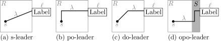
Figure 1: Illustration of leader types. Type-$opo$ leaders use a track routing area $S$.

The boundary labeling problem then asks for the placement of labels such that (1) each label $\ell\in L$ lies outside of $R$ and touches the boundary of $R$, (2) no two labels overlap, and (3) for each site $s$ and its label $\ell$ there is a self-intersection-free curve $\lambda$ in $R$ that starts at $s$ and ends on the boundary of $\ell$. We call the curve $\lambda$ the leader of the site $s$ and its label $\ell$. The end point of $\lambda$ that touches $\ell$ is called the port of $\ell$. Typically, four main parameters, in which the models differ, are distinguished. The label position specifies on which sides of $R$ the labels are placed. The label size may be uniform or individually defined for each label. The port type specifies whether fixed ports or sliding ports are used, i.e., whether the position of a port on its label is pre-defined or flexible. Finally, the leader type restricts the shape of the leaders. As the leader type is the most distinctive feature of the different boundary labeling models in the literature, we examine how this parameter influences the readability. Regarding the other parameters we restrict our attention to one-sided instances whose labels have unit height, lie on the right side of $R$ and have fixed ports. In the following we list the leader types that are most commonly found in the literature.

Let $\lambda$ be a leader connecting a site $s\in P$ with a label $\ell\in L$, and let $r$ be the side of $R$ that is touched by $\ell$. An $s$-leader consists of a single straight ($s$) line segment; see Fig. 1(a). A $po$-leader consists of two line segments, the first, starting at $s$, is parallel ($\mathrm{p}$) to $r$ and the second segment is orthogonal ($\mathrm{o}$) to $r$; see Fig. 1(b). A $do$-leader consists of two line segments, the first, starting at $s$, is diagonal ($\mathrm{d}$) at some angle $\alpha$ (typically $\alpha=45^{\circ}$) relative to $r$ and the second segment is orthogonal ($\mathrm{o}$) to $r$; see Fig. 1(c). An $opo$-leader consists of three line segments, the first, starting at $s$, is orthogonal ($\mathrm{o}$) to $r$, the second is parallel ($\mathrm{p}$) to $r$, and the third segment is orthogonal ($\mathrm{o}$) to $r$; see Fig. 1(d). In case that $opo$-leaders are considered, each leader has its two bends in a strip $S$ next to $r$ whose width is large enough to accommodate all leaders with a minimum pairwise distance of the $p$-segments. The strip $S$ is called the track-routing area of $R$. In the remainder of this paper, we call a labeling based on $s/po/do/opo$-leaders an $s/po/do/opo$-labeling.

Following Tufte’s minimum-ink principle [21], the most common objective in boundary labeling is to minimize the total leader length, which means minimizing the total overlay of leaders with the given figure. Further, to increase readability of the labelings, all models usually require that no two leaders cross each other.

Related Work.

The algorithmic problem of boundary labeling was introduced at GD 2004 by Bekos et al. [7]. They presented efficient algorithms for models based on $po$-, $opo$- and $s$-leaders. As objective functions they considered minimizing the number of bends and the total leader length. While for $opo$-leaders the labels may lie on one, two, or four sides of $R$, the labels for $po$-leaders may lie only on one or on two opposite sides of $R$. In 2005 based on a manual analysis of hand-drawn illustrations (e.g., anatomic atlases), Ali et al. [1] introduced criteria for boundary labeling concerning readability, ambiguity and aesthetics. Based on these they presented force-based heuristics for labeling figures using $s$-leaders and $po$-leaders. In 2006 Bekos et al. considered $opo$-labelings such that labels appear in multiple stacks besides $R$ [5]. Boundary labeling using $do$-leaders has been introduced by Benkert et al. [8] in 2009. They investigated algorithms minimizing a general badness function on $do$- and $po$-leaders and, furthermore, gave more efficient algorithms for the case that the total leader length is minimized. In 2010 Bekos et al. [3] presented further algorithms for $do$-leaders and similarly shaped leaders. Further, Bekos et al. [6] considered $opo$-labelings such that the sites may float within predefined polygons in $R$. Nöllenburg et al. [20] considered $po$-labelings for a setting that supports interactive zooming and panning. In 2011 Gemsa et al. [10] studied the labeling of panorama images using vertical $s$-leaders. Leaders based on Beziér curves and $s$-leaders are further considered in the context of labeling focus regions by Fink et al. [9] (2012). Further, in 2013 Kindermann et al. [13] considered $po$-labelings for the cases that the labels lie on two adjacent sides, or on more than two sides. In 2014 Huang et al. [11] investigated $opo$-labelings with flexible label positions.

Boundary labeling has also been combined in a mixed model with internal labels, i.e., labels that are placed next to the sites [17, 4, 18]. Many-to-one boundary labeling is a further variant, where each label may connect to multiple sites [16, 14, 2]. Finally, boundary labeling has also been considered in the context of text annotations [15, 12].

Table 1: Summary of related work broken down into the considered leader types. The considered leader types are marked by $\times$. If a natural extension of a leader type has been investigated, then it is marked by $\star$.

Year	Reference	Leader Type
		$s$	$po$	$do$	$opo$	other
2004	Bekos et al.[7]	$\times$	$\times$		$\times$
2005	Ali et al.[1]	$\times$	$\times$
2006	Bekos et al.[5]				$\times$
2008	Lin et al.[16]		$\star$		$\star$
2009	Benkert et al.[8]		$\times$	$\times$
	Lin et al.[15]				$\times$	$\times$
2010	Bekos et al.[3]			$\times$		$\times$
	Bekos et al.[6]				$\times$
	Lin [14]				$\star$
	Löffler and Nöllenburg[17]		$\times$
	Nöllenburg et al.[20]		$\times$
2011	Bekos et al.[4]				$\times$
	Gemsa et al.[10]	$\times$
2012	Fink et al.[9]	$\times$				$\times$
2013	Bekos et al.[2]		$\star$
	Kindermann et al.[13]		$\times$
2014	Huang et al.[11]				$\times$
	Kindermann et al.[12]	$\times$	$\times$		$\times$	$\times$
2015	Löffler et al.[18]			$\times$
$\sum$		5	9	3	9	4

In total we found three papers studying $do$-leaders, nine studying $opo$-leaders, nine studying $po$-leaders, and five papers studying $s$-leaders; see Table 1.

Our Contribution.

While boundary labeling has been extensively investigated from an algorithmic perspective, the research on the readability of the introduced models has been neglected. There exist several user studies on the readability and aesthetics of graph drawings. For example Ware et al. [23] studied how people perceive links in node-links diagrams. However, to the best of our knowledge, there are no studies on the readability of any boundary labeling models. In this paper we present the first user study on readability aspects of boundary labeling. When reading a boundary labeling the viewer typically wants to find for a given site its corresponding label, or vice versa. Hence, a well readable labeling must facilitate this basic two-way task such that it can be performed fast and correctly. We call this the assignment task. In this paper we investigate the assignment task with respect to the four most established models, namely models using $s$-, $po$-, $opo$- and $do$-leaders, respectively. To keep the number of parameters small, we refrained from considering other types of leaders. We conducted a controlled user study with 31 subjects. Further, we interviewed eight participants about their personal assessment of the leader types. We obtained the following main results.

• Type-$opo$ leaders lag behind the other leader types in all considered aspects.

• In the assignment task, $do$-, $po$- and $s$-leaders have similar error rates, but $po$-leaders have significantly faster response times than $do$- and $s$-leaders.

• The participants prefer the leader types in the order $do$, $po$, $s$ and $opo$.

2 Research Questions

As argued before, a well readable boundary labeling must allow the viewer to quickly and correctly assign a label to its site and vice versa. More specifically, the leader $\lambda$ connecting the label with its site must be easily traceable by a human. We hypothesize that both the response time and the error rate of the assignment task significantly depend on other leaders running close to and parallel to $\lambda$ in the following sense. The more parallel segments closely surround $\lambda$, the more the response time and the error rate of the assignment task increase.

However, we did not directly investigate this hypothesis, but we derived from it two more concrete hypotheses that are based on the four leader types. These were then investigated in the user study. To that end, we additionally observe, that in medical figures the density of the sites varies. Both may occur, figures containing a dense set of sites, where the sites are placed closely to each other, and figures containing a sparse set of sites, where the sites are dispersed. We now motivate the hypothesis as follows.

By definition of the models, the number of parallel leader segments in $do$-, $po$- and $opo$-labelings is linear in the number of labels per leader, because each pair of leaders has at least one pair of parallel segments. For $opo$-labelings each pair of leaders even has up to three pairs of parallel segments. Additionally, the spacing of the first orthogonal segments of $opo$-leaders is determined by the $y$-coordinates of the sites rather than by the (more regularly spaced) $y$-coordinates of the label ports as in $po$- and $do$-labelings. In contrast, in an $s$-labeling the leaders typically have different slopes, so that (almost) no parallel line segments occur. In fact, it is known that the human eye can distinguish angular differences as small as $10^{\prime\prime}\approx 0.003^{\circ}$ [22]. Hence, leaders of $do$-, $po$- and $opo$-labelings, in particular for a dense set of sites, are closely surrounded by parallel segments, while $s$-leaders for such a set have very different slopes. We therefore propose the next hypothesis.

1. For instances containing a dense set of sites,

   1. the assignment task on $s$-labelings has a significantly smaller response time and error rate than on $do$-, $po$-, and $opo$-labelings.

   2. the assignment task on $do$- and $po$-labelings has a significantly smaller response time and error rate than on $opo$-labelings.

Considering a sparse set of sites, $do$- and $po$-labelings still have many parallel line segments, but this time they are more dispersed. This is normally not true for $opo$-leaders because the actual routing of those leaders occurs in a thin routing area at the boundary of $R$. Hence, we propose the next hypothesis.

1. For instances containing a sparse set of sites, the assignment task on $opo$-labelings has a significantly greater response time and error rate than on $do$-, $po$-, and $s$-labelings.

In summary, we expect that $opo$-labelings perform worse than the other three, that $do$- and $po$-labelings perform similar, and that $s$-labelings perform best.

3 Design of the Experiment

This section presents the tasks, the stimuli, and the experimental procedure that we used to conduct the user study.

Tasks.

In order to test our hypotheses we presented instances of boundary labeling to the participants and asked them to perform the following two tasks.

1. Label-Site-Assignment ($\mathrm{T}_{\mathrm{S}}$): In an instance containing a highlighted label select the related site.

2. Site-Label-Assignment ($\mathrm{T}_{\mathrm{L}}$): In an instance containing a highlighted site select the related label.

Stimuli.

The stimuli are automatically generated boundary labelings, each using the same basic drawing style. In order to remove confounding effects between background image and leaders we use a plain light blue background. Points, leaders and label texts are drawn in the same style and in black color. Highlighted points are drawn as slightly larger yellow-filled squares with black boundary rather than small black disks. Highlighted labels are shown as white text on a dark gray background. Figure 2 exemplarily shows four stimuli.

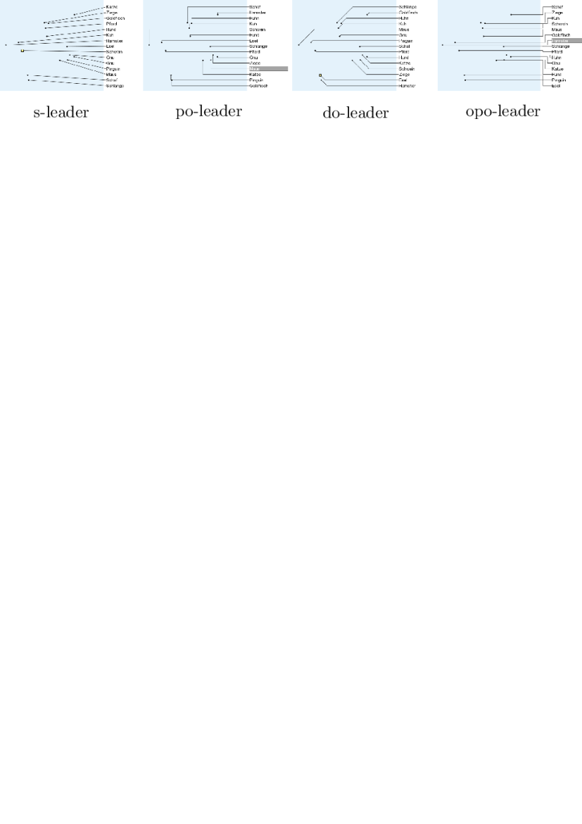
Figure 2: Examples of stimuli for both tasks and all four leader types.

For all instances we defined $R$ to be a rectangle of $500\times 750$ pixels. In addition to the four leader types as the main factor of interest, we identified three secondary factors that may have an impact on the resulting labelings. This yields four parameters to classify an instance. The first parameter is the number $\mathcal{N}=\{15,30\}$ of sites that are contained in the instance. We have chosen $15$ sites to obtain small instances and $30$ sites to obtain large instances, which are typical numbers, e.g., for medical drawings. The second parameter is the distribution $\mathcal{D}=\{\mathrm{D}_{\mathrm{U}},\mathrm{D}_{3},\mathrm{D}_{10}\}$ that is used for randomly placing the sites in $R$. We define $\mathrm{D}_{\mathrm{U}}$ to be a uniform distribution. This distribution yields instances whose sites are dispersed in $R$ without having a certain spatial structure. However, considering, e.g., medical drawings, the instances often consist of spatial clusters. We model such a single cluster by a normal distribution. More precisely, we define $\mathrm{D}_{3}$ and $\mathrm{D}_{10}$ to be normal distributions with mean $\mu=(250,375)$ at the center of $R$, and variance $\sigma=3000$ and $\sigma=10000$ in both directions, respectively. Hence, $\mathrm{D}_{3}$ yields instances consisting of a dense set of sites, while $\mathrm{D}_{10}$ yields instances consisting of a sparse set of sites. In order to avoid cluttered sets of sites and degenerated instances, where sites lie too close to the boundary of $R$, we rejected instances where any two sites have less than $10$ pixels distance or where a site has less than $30$ pixels distance to the boundary of $R$. The third parameter is the applied leader type $\mathcal{T}=\{do,opo,po,s\}$ as defined above. Finally, the fourth parameter $\mathcal{R}=\{0.3,0.6,0.9\}$ can be seen as a difficulty level and specifies which leader of the instance should be selected for the tasks $\mathrm{T}_{\mathrm{S}}$ and $\mathrm{T}_{\mathrm{L}}$. This is accomplished by scoring each leader with respect to how much ink is close to it in the drawing. More specifically, ranking a leader $\lambda_{i}$ is done as follows: For every other leader $\lambda_{j}$, points are linearly sampled on $\lambda_{j}$ with one pixel distance from each other. For each such point, the minimum distance $d$ to $\lambda_{i}$ is computed. Then, every sample point contributes $\frac{1}{d^{2}}$ to the ink score of $\lambda_{i}$. The parameter $r\in\mathcal{R}$ then selects the leader $\lambda$ whose ink score is the $r$-quantile among the ink scores of all leaders in the instance. Thus the parameter $\mathcal{R}$ lets us control the relative difficulty of the chosen leader.

The parameter space $\mathcal{N}\times\mathcal{D}\times\mathcal{T}\times\mathcal{R}$ gives us the possibility to cover a large variety of different instances. For each of the 72 possible choices of parameters $(n,d,t,r)\in\mathcal{N}\times\mathcal{D}\times\mathcal{T}\times\mathcal{R}$ we have generated two instances $I_{1}$ and $I_{2}$, one for each task. To that end, we used the property that a leader of any of the four types is uniquely determined by the location of its port and site. Hence, using integer linear programming (ILP) we computed a length minimal labeling of the chosen leader type such that the labels are placed to the right side of $R$ using one of $150$ equally spaced ports each. The ILP further ensures that the subset of chosen ports does not create overlapping labels and that no two leaders cross. In each instance each label is randomly chosen from a pre-defined set of German animal names. For $opo$-labelings, the track routing area and the routing of the leaders is chosen such that the $p$-segments of any two leaders have horizontal distance of at least $10$ pixels from each other.

It will occur in the instances that leaders lie closely together, e.g., see $opo$-labeling in Fig. 2. However, we do not enforce minimum spacing between leaders because neither any of the studied models nor any of the discussed algorithms enforce minimum spacing explicitly. In fact, a fixed minimum leader spacing may even lead to infeasible instances for certain leader types.

Procedure.

The study was run as a within-subject experiment. Four experimental sessions were held in our computer lab at controlled lighting with 12 identical machines and screens using a digital questionnaire in German language. After agreeing to a consent form, each participant first completed a tutorial explaining him or her the tasks $\mathrm{T}_{\mathrm{S}}$ and $\mathrm{T}_{\mathrm{L}}$ on four instances, each containing one of the four labeling types. Participants were instructed to answer the questions as quickly and as accurately as possible. Afterwards, the actual study started presenting the 144 stimuli to the participant one at a time. Each stimulus was revealed to the participant, after he or she clicked a button in the center of the screen using the mouse. Hence, at the beginning of each task the mouse pointer was always located at the same position. Then he or she performed the task by selecting a label or site using the mouse.

The stimuli were divided into 12 blocks consisting of 12 stimuli each. Each block either contained stimuli only for $\mathrm{T}_{\mathrm{S}}$ or only for $\mathrm{T}_{\mathrm{L}}$. For each participant the stimuli were in random order, but in alternating blocks, i.e., after completing a block for $\mathrm{T}_{\mathrm{S}}$ a block for $\mathrm{T}_{\mathrm{L}}$ was presented, and vice versa. Between two successive blocks a pause screen stated the task for the next block and participants were asked to take a break of at least 15 seconds before continuing.

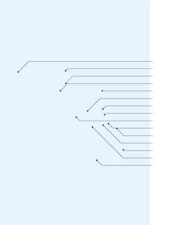
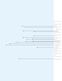
$do$-leaders	$opo$-leaders
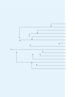
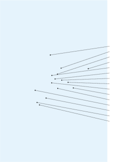
$po$-leaders	$s$-leaders

Figure 7: Instances presented as examples next to the personal preference questions.

Especially for professional printings, e.g. for atlases of human anatomy, not only the figure’s readability, but also its aesthetics is seen to be of great importance. Further, assigning a label to its site (or vice versa), the viewer should be able to assess whether he or she has done this correctly. We therefore asked all participants about their personal assessment of the aesthetics and readability of the leader types after completing the 144 performance trials. We presented the same four selected instances of the four leader types to each participant. To that end, we selected an instance for each leader type $t\in\mathcal{T}$ based on the 144 instances generated for the tasks $\mathrm{T}_{\mathrm{S}}$ and $\mathrm{T}_{\mathrm{L}}$. We score each instance by the sum of its leaders’ ink scores. Among all instances with leader type $t\in\mathcal{T}$ and 15 sites, we selected the median instance $I$ with respect to the instance scores of that subset. Hence, for each type of leader we obtain a moderate instance with respect to our difficulty measure; see Fig. 7 in the appendix. Each participant was asked to rate the different leader types using German school grades on a scale from 1 (excellent) to 6 (insufficient), where grades 5 and 6 are both fail-grades, color=yellow!40]MN: wenn platz ist alle noten ausschreiben by answering the following questions.

1. How do you rate the appearance of the leader types?

2. For a highlighted site, how easy is it for you to find the corresponding label?

3. For a highlighted label, how easy is it for you to find the corresponding site?

We further conducted interviews with eight participants after the experiment, in which they justified their grading.

4 Results

In total 31 students of computer science in the age between 20 and 30 years completed the experiment, six of them were female and 25 were male. We also asked whether they have fundamental knowledge about labeling figures and maps, which was affirmed by only two participants.

4.1 Performance Analysis

For each of the 144 trials we recorded both the response time and the correctness of the answer, which allows for analyzing two separate quantitative performance measures. Response times were measured from the time a stimulus was revealed until the participant clicks to give the answer. Response times are normalized per participant by his/her median response time to compensate for different reaction times among participants. We split the data into four groups by leader type, and call them $\mathcal{DO}$, $\mathcal{PO}$, $\mathcal{S}$ and $\mathcal{OPO}$, respectively. color=yellow!40]MN: falls noch Zeit ist: die Reihenfolge von vorne ist S, PO, DO, OPO; wollten wir das nicht durchs PAper so durchziehen? Ist aber nur ein nice-to-have, spätestens für die final version.

We applied repeated-measures Friedman tests with post-hoc Dunn-Bonferroni pairwise comparisons in SPSS between the four groups to find significant differences in the performance data at a significance level of $p=0.05$. We chose a non-parametric test since our data are not normally distributed. We report the detailed test results in Table 5 (response times) and Table 6 (success rates) in the appendix and summarize the main findings in the following paragraphs.

Response Times.

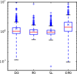
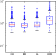
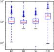
$\mathrm{T}_{\mathrm{S}}$	$\mathrm{T}_{\mathrm{L}}$	Large	Small

(a) Response times over all tasks (OPT).

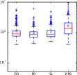
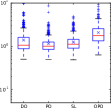
$\mathrm{T}_{\mathrm{S}}$	$\mathrm{T}_{\mathrm{L}}$	Large	Small

(b) Response times over all correctly processed tasks (CPT).

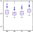
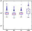
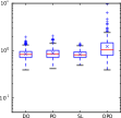
Dense	Sparse	Uniform

(c) Response times over all correctly processed tasks (CPT).

Figure 5: Normalized response times (on log-scale) broken down to different parameters. Mean values are indicated by a bold ’x’. The corresponding significances are found in Table 5. Smaller values are better than higher values.

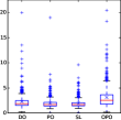
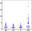
$\mathrm{T}_{\mathrm{S}}$	$\mathrm{T}_{\mathrm{L}}$	Large	Small

(a) Response times in seconds over all tasks (OPT) broken into large and small instances as well as instances for task $\mathrm{T}_{\mathrm{S}}$ and $\mathrm{T}_{\mathrm{L}}$.

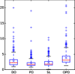
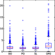
Dense	Sparse	Uniform	All

(b) Response times in seconds over all tasks (OPT) broken into dense, sparse and uniform instances as well as all instances.

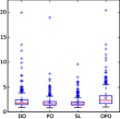
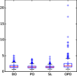
$\mathrm{T}_{\mathrm{S}}$	$\mathrm{T}_{\mathrm{L}}$	Large	Small

(c) Response times in seconds over all correctly processed tasks (CPT) broken into large, small instances as well as instances for task $\mathrm{T}_{\mathrm{S}}$ and $\mathrm{T}_{\mathrm{L}}$.

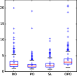
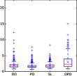
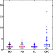
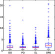
Dense	Sparse	Uniform	All

(d) Response times in seconds over all correctly processed tasks (CPT) broken into dense, sparse and uniform instances as well as all instances.

Figure 6: Absolute response times (in seconds) broken down to different parameters. Mean values are indicated by a bold ’x’. The corresponding significances are found in Table 5. Smaller values are better than higher values.

Figure 3a shows the normalized response times broken down into the three considered distributions $\mathrm{D}_{3}$, $\mathrm{D}_{10}$ and $\mathrm{D}_{\mathrm{U}}$, which yield dense, sparse and uniform sets of sites; the corresponding mean times are found in Table 3, and further plots for both normalized and absolute response times are found in Fig. 5 and Fig. 6 in the appendix. We obtained the following results. Among all leader types, $opo$-leaders have the highest response time. In particular for dense and sparse sets of sites the mean response time is up to a factor 1.8 worse than for the others. For uniform sets we obtain a factor of up to 1.5. Further, for any distribution the measured differences are significant. Comparing the response times of the remaining leader types we obtain the order $po<s<do$ with respect to increasing mean response time. For uniform sets we did not measure any pairwise significant difference between $do$, $po$ and $s$ leaders. However, for dense and sparse sets we obtained the significant differences as shown in Fig. 3a. We emphasize that for $po$- and $s$-leaders significant differences are measured for sparse, but not for dense sets of sites. In contrast $do$- and $s$-leaders have significant differences for dense sets, but not for sparse sets. Further, $po$- and $do$-leaders have significant differences in both dense and sparse sets. Altogether, this justifies the ranking $po<s<do$ w.r.t. increasing mean response time.

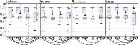
(a) Normalized response times (logarithmic scale). Smaller values are better than higher values.

(b) Success rates. Higher values are better than smaller values.

Figure 3: Performance results broken down to dense, sparse and uniform sets as well as to large instances (30 sites). Mean values are indicated by ’x’. Arcs at the bottom show significant differences that were found ($p=0.05$).

Comparing the instances in terms of $\mathrm{T}_{\mathrm{S}}$ and $\mathrm{T}_{\mathrm{L}}$, the mean response time of $\mathrm{T}_{\mathrm{L}}$ is slightly lower than that of $\mathrm{T}_{\mathrm{S}}$. Filtering out incorrectly processed tasks does not change the mean response time much and similar results are obtained; see Table 3. The mean response times of large instances (any instance with 30 sites and dense, sparse or uniform distribution) are similar to those of dense sets, and the mean response times of small instances (any instance with 15 sites and dense, sparse or uniform distribution) are similar to those of uniform sets.

Accuracy.

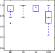
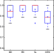
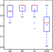
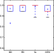
$\mathrm{T}_{\mathrm{S}}$	$\mathrm{T}_{\mathrm{L}}$	Large	Small

Figure 4: Success rates broken down to different parameters. Mean values are indicated by a bold ’x’. The corresponding significances are found in Table 6. Higher values are better than smaller values.

We computed for each leader type and each participant the proportion of instances of that type that the participant solved correctly; see Fig. 3b and Table 4. Further plots are found in Fig. 4 in the appendix. For dense and sparse sets of sites we observe that $\mathcal{OPO}$ has success rates around $86\%$, while the other groups have success rates greater than $93\%$. In particular the differences between success rates of $opo$-leaders and the remaining types are up to $11\%$ and $13\%$ for dense and sparse sets, respectively. Any of these differences is significant, while between $\mathcal{PO}$, $\mathcal{DO}$ and $\mathcal{S}$ no significant accuracy differences were measured. For uniform sets of sites, on the other hand, no significant differences were measured and any group has a success rate greater than $95\%$. Hence, it appears that uniform sets of sites produce easily readable labelings with any leader type – unlike dense and sparse instances.

Considering large and small instances separately, the group $\mathcal{OPO}$ has a decreased success rate ($81\%$), while the other groups remain almost unchanged ($>93\%$), which yields for $\mathcal{PO}$ and $\mathcal{OPO}$ a difference of $16\%$. For small instances no significant differences were measured. Comparing the instances by tasks $\mathrm{T}_{\mathrm{S}}$ and $\mathrm{T}_{\mathrm{L}}$, the success rate of $\mathrm{T}_{\mathrm{S}}$ is slightly better than that of $\mathrm{T}_{\mathrm{L}}$ except for $\mathcal{OPO}$. For the mean response times the contrary is observed.

4.2 Preference Data

Table 2 shows the average grades given by the participants with respect to the three questions Q1–Q3. Concerning the general aesthetic appeal (question Q1) leaders of type $do$ received the best grades (1.8), followed by $po$-leaders (grade 2.3). The participants did not particularly like the appearance of $s$-leaders (grade 3.3) and generally disliked $opo$-leaders (grade 4.6). Table 7 in the appendix lists the detailed percentages of participants who graded a particular leader type better,

Table 2: Average grades given by the participants with respect to questions Q1–Q3. Smaller values are better than higher values.

	$do$	$opo$	$po$	$s$
Q1	1.8	4.6	2.3	3.3
Q2	2.0	4.6	2.1	2.4
Q3	1.7	4.3	2.3	2.4

equally, or worse than another type. In addition to the general impression from the average grades it is worth mentioning that between the two most preferred leader types $do$ and $po$ 48.4% preferred $do$ over $po$ and 38.7% gave the same grades to both leader types. Compared to the $s$-leaders, a great majority ($>$ 80%) strictly prefers both $do$- and $po$-leaders. In the interviews seven out of eight participants stated that $opo$-leaders are “confusing, because leaders closely pass by each other”. They disliked the long parallel segments of $opo$-leaders. Further, some participants remarked that $opo$-leaders “consist of too many bends”. For six participants $s$-leaders were “chaotic and unstructured”, unlike $do$- and $po$-leaders. Five participants said that they liked the flat bend of $do$-leaders more than the sharp bend of $po$-leaders. One participant stated that “$po$-leaders seem to be more abstract than $do$-leaders”. Further, it was said that “the ratio of the segments’ lengths is less balanced for $po$- than $do$-leaders.”

For question Q2 (site-to-label) $do$- and $po$-leaders were ranked best (see Table 2), followed by $s$ and more than two grades behind by $opo$, whereas for question Q3 (label-to-site) $do$-leaders are further ahead of $po$- and $s$-leaders, both of which received similar grades, and are again about two grades ahead of $opo$-leaders. For questions Q2 and Q3 the most striking observation is that type-$s$ leaders received much better results (almost a full grade point better) than for Q1. This is in strong contrast to the other three leader types, which received grades in the same range as for Q1. This indicates that the participants perceived straight leaders as being well readable during the experiment, but still did not produce very appealing labelings. In the interviews participants stated that “$opo$-leaders are hard to read because of leaders lying close to each other.” They negatively observed that $opo$-leaders “may not be clearly distinguished”, but assessed the “simple shape of $s$-leaders to be easily legible.” Further, they positively noted that “the distances between $do$-leaders seem to be greater than for other types” and that “$po$-leaders are easier to follow than other types”.

It is remarkable that the participants rated $do$-leaders best, while they ranked third in our performance test. We conjecture that the participants overestimate the performance of $do$-leaders, because they like their aesthetics. For $s$-leaders the reverse is true. In contrast, their assessment on $po$- and $opo$-leaders corresponds more closely with the result of our performance test.

In summary, $do$-leaders obtained the best subjective ratings. The regularly shaped $po$- and $do$-leaders both scored better than the irregular and less restricted $s$-leaders. For any of the three questions $opo$-leaders were rated a lot worse than the others, which is, according to the interviews, mostly due to the frequent occurrence of many nearby leaders running closely together.

5 Discussion

In Section 2 we hypothesized that labelings with many parallel leaders lying close to each other have a significant negative effect on response times and accuracy. Our results from Section 4.1 indeed support hypotheses (H1b) and (H2), which said that the assignment task has a significantly smaller response time and error rate for $do$- and $po$-labelings than for $opo$-labelings in dense (H1b) and also sparse sets of sites (H2). Hypothesis (H2) was claimed to also hold for $s$-labelings versus $opo$-labelings, which is confirmed by the experiment as well. While greater response times may still be acceptable in some cases, the significantly lower accuracy clearly restricts the usability of $opo$-leaders. Only for small numbers of sites and uniform distributions $opo$-leaders have comparable success rates to the other leader types. This judgment is strengthened further by the preference ratings. On average the participants graded $opo$-leaders between 4 (sufficient) and 5 (poor) in all concerns. The main reason given in the interviews was that $opo$-labelings are confusing due to many leaders closely passing by each other.

However, our results falsified hypothesis (H1a), which claimed that for dense instances type-$s$ leaders perform significantly better than the other three leader types. Rather we gained unexpected insights into the readability of boundary labeling. While we had expected that due to their simple shape and easily distinguishable slopes $s$-leaders will perform better than all other types of leaders, we could not measure significant differences between $po$-leaders and $s$-leaders. Interestingly, on average, the participants graded $po$-leaders better than $s$-leaders in all examined concerns, in particular with respect to their aesthetics (Q1). This is emphasized by the statements given by the participants that $po$-labelings appear structured while $s$-labelings were perceived as chaotic. Comparing $do$- and $s$-leaders we measured some evidence for (H1a), namely that the assignment task has significantly smaller response times for $s$- than for $do$-leaders. However, the success rates did not differ significantly.

We summarize our main findings regarding the four leader types as follows:

1. $do$-leaders perform best in the preference rankings, but concerning the assignment tasks they perform slightly worse than $po$- and $s$-leaders.

2. $opo$-leaders perform worst, both in the assignment tasks and the preference rankings. They are applicable only for small instances or for uniformly distributed sites.

3. $po$-leaders perform best in the assignment tasks, and received good grades in the preference rankings.

4. $s$-leaders perform well in the assignment tasks, but not in the preference rankings. The participants dislike their unstructured appearance.

We can generally recommend $po$-leaders as the best compromise between measured task performance and subjective preference ratings. For aesthetic reasons, it may also be advisable to use $do$-leaders instead as they have only slightly lower readability scores but are considered the most appealing leader type.

An interesting question is why type-$s$ leaders (which showed good task performance) are frequently used by professional graphic designers, e.g., in anatomical drawings, although they were not perceived as aesthetically pleasing in our experiment. One explanation may be that our experiment judged all leader types on an empty background, where the leaders receive the entire visual attention of a viewer. In reality, the labeled figure itself is the main visual element and the leaders should be as unobtrusive as possible and not interfere with the figure. It would be necessary to conduct further experiments to assess the influence and interplay of image and leaders on more complex readability tasks.

Another interesting follow-up question is whether the chosen objective function produces actually the most aesthetic and most readable labelings. Despite being the predominant objective function in the literature on boundary labeling, simply minimizing the total leader length most certainly does not capture all relevant quality criteria.

Acknowledgments. We thank Helen Purchase and Janet Siegmund for their advice on the statistical data analysis.

Appendix A Data

Table 3: Mean normalized response times for overall processed tasks and for correctly processed tasks. The times are broken down into dense, sparse and uniform sets of sites, into large and small instances, as well as the tasks $\mathrm{T}_{\mathrm{S}}$ and $\mathrm{T}_{\mathrm{L}}$.

	Overall processed tasks				Correctly processed tasks
	$\mathcal{DO}$	$\mathcal{PO}$	$\mathcal{S}$	$\mathcal{OPO}$	$\mathcal{DO}$	$\mathcal{PO}$	$\mathcal{S}$	$\mathcal{OPO}$
Dense	1.564	1.161	1.266	2.122	1.552	1.142	1.262	2.020
Sparse	1.143	0.981	1.063	1.813	1.132	0.980	1.065	1.667
Uniform	0.852	0.885	0.836	1.287	0.855	0.894	0.837	1.231
Large	1.425	1.167	1.262	2.201	1.405	1.158	1.262	2.083
Small	0.949	0.852	0.848	1.281	0.948	0.854	0.850	1.239
$\mathrm{T}_{\mathrm{S}}$	1.276	1.083	1.074	1.748	1.266	1.086	1.072	1.602
$\mathrm{T}_{\mathrm{L}}$	1.098	0.936	1.037	1.743	1,081	0.922	1.032	1.648

Table 4: Mean success rates. The rates are broken down into dense, sparse and uniform sets of sites, into large and small instances, as well as the tasks $\mathrm{T}_{\mathrm{S}}$ and $\mathrm{T}_{\mathrm{L}}$.

	$\mathcal{DO}$	$\mathcal{PO}$	$\mathcal{S}$	$\mathcal{OPO}$
Dense	0.930	0.973	0.952	0.860
Sparse	0.957	0.987	0.978	0.855
Uniform	0.981	0.973	0.987	0.952
Large	0.943	0.973	0.945	0.814
Small	0.970	0.982	0.988	0.964
$\mathrm{T}_{\mathrm{S}}$	0.959	0.991	0.982	0.886
$\mathrm{T}_{\mathrm{L}}$	0.953	0.964	0.962	0.892

Table 5: Results of the Dunn-Borferroni test on the response times of the respective pairs of groups. The values estimate the likelihood that both respective sample groups are from the same population. A value $<0.05$ is treated as statistically significant difference (marked green). OPT: all processed tasks. CPT: correctly processed tasks only. $\mathrm{T}_{\mathrm{S}}$/$\mathrm{T}_{\mathrm{L}}$: Restricted to instances of task $\mathrm{T}_{\mathrm{S}}$/$\mathrm{T}_{\mathrm{L}}$. Dense/Sparse/Uniform: Restricted to instances of distribution dense/sparse/uniform. Large/Small: Restricted to instances containing 30 and 15 sites, respectively.

	$\mathcal{PO}$-$\mathcal{S}$		$\mathcal{S}$-$\mathcal{DO}$		$\mathcal{PO}$-$\mathcal{DO}$		$\mathcal{DO}$-$\mathcal{OPO}$		$\mathcal{S}$-$\mathcal{OPO}$		$\mathcal{PO}$-$\mathcal{OPO}$
OPT:$\mathrm{T}_{\mathrm{S}}$	$1.0$		$<10^{-3}$		$<10^{-3}$		$<10^{-3}$		$<10^{-3}$		$<10^{-3}$
OPT:$\mathrm{T}_{\mathrm{L}}$	$0.010$		$0.382$		$<10^{-3}$		$<10^{-3}$		$<10^{-3}$		$<10^{-3}$
OPT:Dense	$0.415$		$<10^{-3}$		$<10^{-3}$		$<10^{-3}$		$<10^{-3}$		$<10^{-3}$
OPT:Sparse	$0.001$		$1.0$		$<10^{-3}$		$<10^{-3}$		$<10^{-3}$		$<10^{-3}$
OPT:Uniform	$0.263$		$1.0$		$0.129$		$<10^{-3}$		$<10^{-3}$		$<10^{-3}$
OPT:Large	$0.335$		$0.098$		$<10^{-3}$		$<10^{-3}$		$<10^{-3}$		$<10^{-3}$
OPT:Small	$1.0$		$0.001$		$<10^{-3}$		$<10^{-3}$		$<10^{-3}$		$<10^{-3}$
CPT:$\mathrm{T}_{\mathrm{S}}$	$1.0$		$0.001$		$0.001$		$<10^{-3}$		$<10^{-3}$		$<10^{-3}$
CPT:$\mathrm{T}_{\mathrm{L}}$	$0.281$		$0.174$		$<10^{-3}$		$<10^{-3}$		$<10^{-3}$		$<10^{-3}$
CPT:Dense	$1.0$		$<10^{-3}$		$<10^{-3}$		$<10^{-3}$		$<10^{-3}$		$<10^{-3}$
CPT:Sparse	$0.002$		$1.0$		$0.003$		$<10^{-3}$		$<10^{-3}$		$<10^{-3}$
CPT:Uniform	$0.125$		$1.0$		$0.135$		$<10^{-3}$		$<10^{-3}$		$<10^{-3}$
CPT:Large	$1.0$		$0.221$		$0.013$		$<10^{-3}$		$<10^{-3}$		$<10^{-3}$
CPT:Small	$1.0$		$0.001$		$<10^{-3}$		$<10^{-3}$		$<10^{-3}$		$<10^{-3}$

Table 6: Results of the Dunn-Borferroni test on the success rates of the respective pairs of groups. The values estimate the likelihood that both respective sample groups are from the same population. A value $<0.05$ is treated as statistically significant difference (marked green). $\mathrm{T}_{\mathrm{S}}$/$\mathrm{T}_{\mathrm{L}}$: Restricted to instances of task $\mathrm{T}_{\mathrm{S}}$/$\mathrm{T}_{\mathrm{L}}$. Dense/Sparse/Uniform: Restricted to instances of distribution dense/sparse/uniform. Large/Small: Restricted to instances containing 30 and 15 sites, respectively.

	$\mathcal{PO}$-$\mathcal{S}$		$\mathcal{S}$-$\mathcal{DO}$		$\mathcal{PO}$-$\mathcal{DO}$		$\mathcal{DO}$-$\mathcal{OPO}$		$\mathcal{S}$-$\mathcal{OPO}$		$\mathcal{PO}$-$\mathcal{OPO}$
$\mathrm{T}_{\mathrm{S}}$	$1.0$		$1.0$		$0.460$		$<10^{-3}$		$<10^{-3}$		$<10^{-3}$
$\mathrm{T}_{\mathrm{L}}$	$1.0$		$1.0$		$1.0$		$0.001$		$<10^{-3}$		$<10^{-3}$
Dense	$1.0$		$1.0$		$0.330$		$0.019$		$0.001$		$<10^{-3}$
Sparse	$1.0$		$1.0$		$1.0$		$0.001$		$<10^{-3}$		$<10^{-3}$
Uniform	$1.0$		$1.0$		$1.0$		$0.262$		$0.125$		$1.0$
Large	$1.0$		$1.0$		$0.922$		$<10^{-3}$		$<10^{-3}$		$<10^{-3}$
Small	$1.0$		$0.764$		$1.0$		$1.0$		$0.055$		$0.262$

Table 7: Statistics for questions Q1–Q3. The percentage of participants that graded a leader type better ($<$), equally ($=$) or worse ($>$) than another. Majorities are highlighted in bold.

	$do{<}opo$	$do{=}opo$	$do{>}opo$	$do{<}po$	$do{=}po$	$do{>}po$	$do{<}s$	$do{=}s$	$do{>}s$
Q1	100	0	0	48.4	38.7	12.9	90.3	3.2	6.5
Q2	93.5	3.2	3.2	32.3	41.9	25.8	48.4	19.4	32.3
Q3	93.5	6.5	0	54.8	35.5	9.7	48.4	35.5	16.1
	$po{<}opo$	$po{=}opo$	$po{>}opo$	$po{<}s$	$po{=}s$	$po{>}s$	$s{<}opo$	$s{=}opo$	$s{>}opo$
Q1	100	0	0	80.6	3.2	16.1	80.6	6.5	12.9
Q2	96.8	3.2	0	35.5	25.8	38.7	83.9	9.7	6.5
Q3	93.5	3.2	3.2	41.9	16.1	41.9	93.5	3.2	3.2

Appendix B Examples of Stimuli

	Dense		Sparse		Uniform
$\mathcal{PO}$
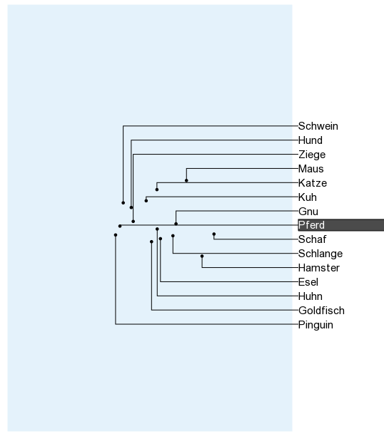
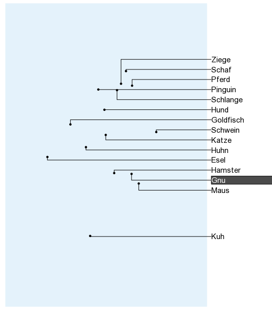
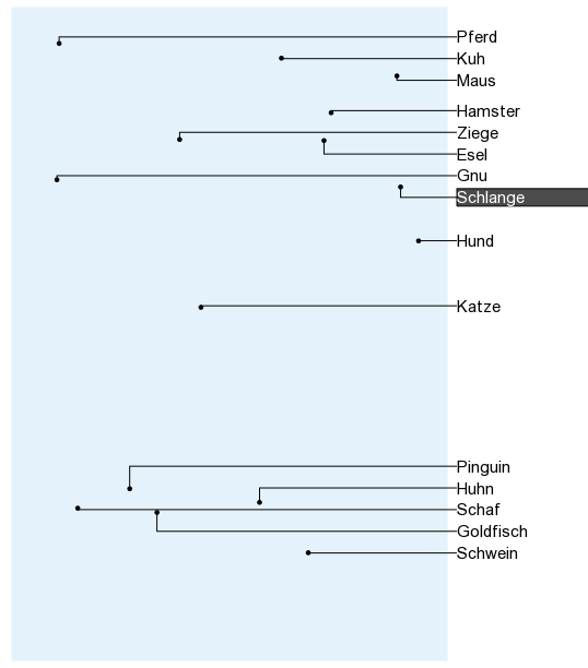
$\mathcal{S}$
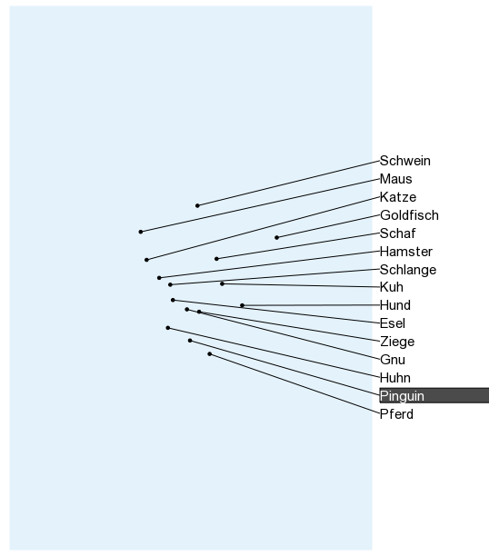
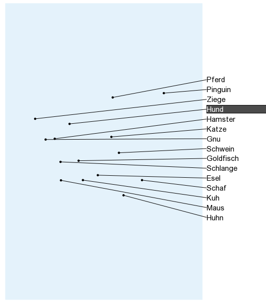
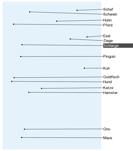
$\mathcal{DO}$
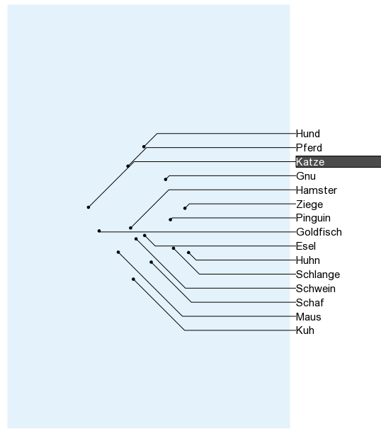
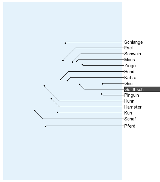
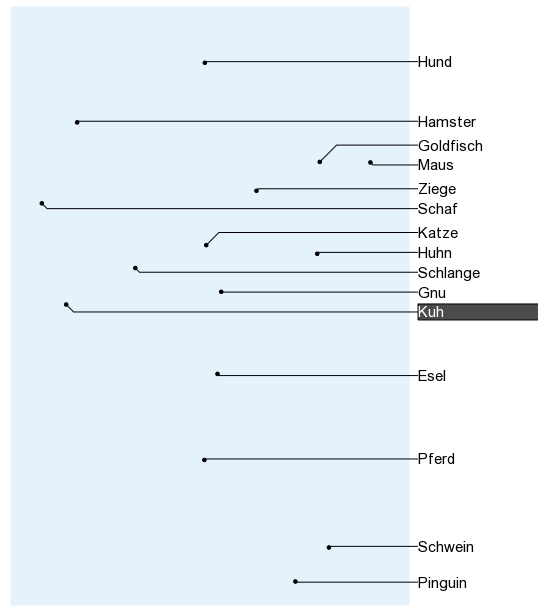
$\mathcal{OPO}$

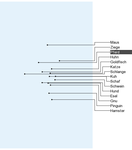
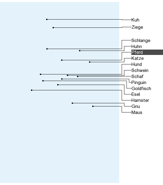
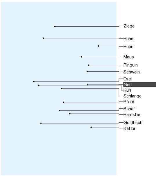
Figure 8: Example stimuli with 15 sites (small), one for each site distribution and for each leader type. Due to formatting the rectangles enclosing the sites may not have same sizes. In the digital questionnaire they had the same size.

	Dense		Sparse		Uniform
$\mathcal{PO}$
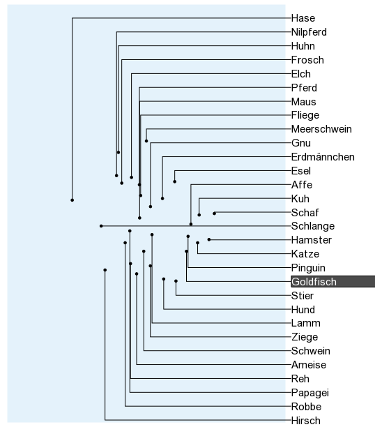
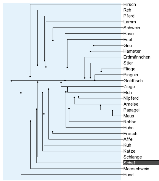
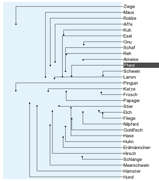
$\mathcal{S}$
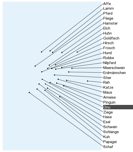
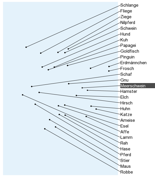
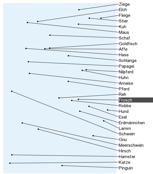
$\mathcal{DO}$
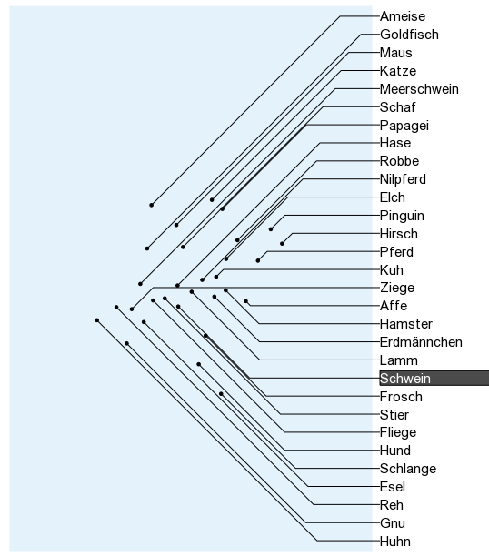
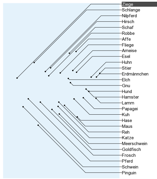
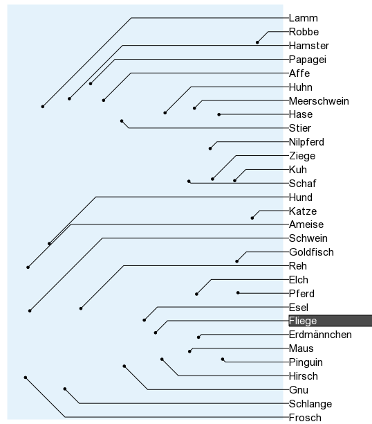
$\mathcal{OPO}$

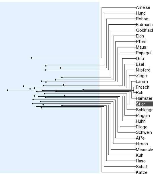
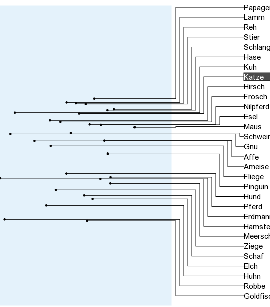
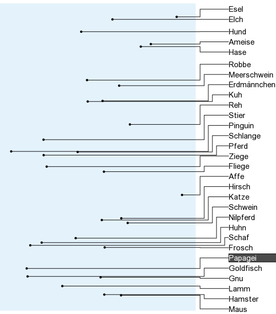
Figure 9: Example stimuli with 30 sites (large), one for each site distribution and for each leader type. Due to formatting the rectangles enclosing the sites may not have same sizes. In the digital questionnaire they had the same size.

References

- [1] K. Ali, K. Hartmann, and T. Strothotte. Label Layout for Interactive 3D Illustrations. Journal of the WSCG, 13(1):1–8, 2005.
- [2] M. Bekos, S. Cornelsen, M. Fink, S.-H. Hong, M. Kaufmann, M. Nöllenburg, I. Rutter, and A. Symvonis. Many-to-one boundary labeling with backbones. In Graph Drawing (GD’13), volume 8242 of LNCS, pages 244–255. Springer, 2013.
- [3] M. A. Bekos, M. Kaufmann, M. Nöllenburg, and A. Symvonis. Boundary labeling with octilinear leaders. Algorithmica, 57(3):436–461, 2010.
- [4] M. A. Bekos, M. Kaufmann, D. Papadopoulos, and A. Symvonis. Combining traditional map labeling with boundary labeling. In I. Cerná et al., editor, SOFSEM 2011, volume 6543 of LNCS, pages 111–122. Springer, Heidelberg, 2011.
- [5] M. A. Bekos, M. Kaufmann, K. Potika, and A. Symvonis. Multi-stack boundary labeling problems. In S. Arun-Kumar and N. Garg, editors, FSTTCS 2006, volume 4337 of LNCS, pages 81–92. Springer, Heidelberg, 2006.
- [6] M. A. Bekos, M. Kaufmann, K. Potika, and A. Symvonis. Area-feature boundary labeling. Comput. J., 53(6):827–841, 2010.
- [7] M. A. Bekos, M. Kaufmann, A. Symvonis, and A. Wolff. Boundary labeling: Models and efficient algorithms for rectangular maps. Comp. Geom. Theory Appl., 36(3):215–236, 2007.
- [8] M. Benkert, H. J. Haverkort, M. Kroll, and M. Nöllenburg. Algorithms for multi-criteria boundary labeling. J. Graph Algorithms Appl., 13(3):289–317, 2009.
- [9] M. Fink, J.-H. Haunert, A. Schulz, J. Spoerhase, and A. Wolff. Algorithms for labeling focus regions. InforVis 2012, 18(12):2583–2592, 2012.
- [10] A. Gemsa, J.-H. Haunert, and M. Nöllenburg. Boundary-labeling algorithms for panorama images. In ACM GIS 2011, pages 289–298, New York, NY, USA, 2011.
- [11] Z. Huang, S. Poon, and C. Lin. Boundary labeling with flexible label positions. In WALCOM 2014, volume 8344 of LNCS, pages 44–55. Springer, 2014.
- [12] P. Kindermann, F. Lipp, and A. Wolff. Luatodonotes: Boundary labeling for annotations in texts. In GD 2014, vol. 8871 of LNCS, pp. 76–88. Springer, 2014.
- [13] P. Kindermann, B. Niedermann, I. Rutter, M. Schaefer, A. Schulz, and A. Wolff. Two-sided boundary labeling with adjacent sides. In WADS 2013, volume 8037 of LNCS, pages 463–474. Springer, 2013.
- [14] C. Lin. Crossing-free many-to-one boundary labeling with hyperleaders. In PacificVis 2010, pages 185–192. IEEE, 2010.
- [15] C. Lin, H. Wu, and H. Yen. Boundary labeling in text annotation. In E. Banissi et al., editor, IV 2009, pages 110–115. IEEE, 2009.
- [16] C.-C. Lin, H.-J. Kao, and H.-C. Yen. Many-to-one boundary labeling. J. Graph Algorithms Appl., 12(3):319–356, 2008.
- [17] M. Löffler and M. Nöllenburg. Shooting bricks with orthogonal laser beams: A first step towards internal/external map labeling. In CCCG 2010, pp. 203–206, 2010.
- [18] M. Löffler, M. Nöllenburg, and F. Staals. Mixed map labeling. In CIAC 2015, volume 9079 of LNCS, pages 339–351. Springer, 2015.
- [19] J. L. Morrison. Computer technology and cartographic change. In D. Taylor, ed., The Computer in Contemporary Cartography. Johns Hopkins Univ. Press, 1980.
- [20] M. Nöllenburg, V. Polishchuk, and M. Sysikaski. Dynamic one-sided boundary labeling. In ACM-GIS 2010, pages 310–319, 2010.
- [21] E. R. Tufte. The Visual Display of Quantitative Information. Graphics Press, 2001.
- [22] C. Ware. Information Visualization: Perception for Design. Morgan Kaufmann, 3rd edition, 2012.
- [23] C. Ware, H. Purchase, L. Colpoys, M. McGill. Cognitive Measurements of Graph Aesthetics J. Infor. Vis., 1(2):103–110, 2002.