A breakpoint detection error function for segmentation model selection and evaluation

Abstract

We consider the multiple breakpoint detection problem, which is concerned with detecting the locations of several distinct changes in a one-dimensional noisy data series. We propose the breakpointError, a function that can be used to evaluate estimated breakpoint locations, given the known locations of true breakpoints. We discuss an application of the breakpointError for finding optimal penalties for breakpoint detection in simulated data. Finally, we show how to relax the breakpointError to obtain an annotation error function which can be used more readily in practice on real data. A fast C implementation of an algorithm that computes the breakpointError is available in an R package on R-Forge.

1 Introduction to segmentation models

The goal of a segmentation model or algorithm is to divide a series of data into distinct segments. A major application of segmentation models is in detecting changes in copy number in cancer, using technologies such as array comparative genomic hybridization (Pinkel et al., 1998). In these noisy biological data sets, the goal of segmentation is to detect the precise base pairs or genomic positions after which there are changes in copy number.

How to evaluate the accuracy of a segmentation model? A new method for supervised segmentation of copy number data was proposed by Hocking et al. (2013), who quantified the segmentation model accuracy using an annotation database containing visually-determined regions with or without breakpoints. This method depends critically on the definition of the visually-determined annotated region database, which is used to compute an annotation error function.

This paper continues this line of research by defining the breakpointError function, which uses the true breakpoints to precisely compute the accuracy of a segmentation model. Also in this paper we demonstrate that the breakpointError is closely related to the annotation error, thus giving a theoretical foundation to the very practical new methods based on visually-determined annotated region databases.

In this introduction, we first discuss a few motivating examples with figures. In Section 2 we discuss related work, and in Section 3 we define the breakpointError. In Section 4 we show an application of the breakpointError, and in Section 5 we discuss its relationship to the annotation error. In general we use bold to denote vectors ($\mathbf{x},\mathbf{\hat{y}}^{k}$) and plain text to denote elements of those vectors ($x_{i},y_{i}^{k}$) and scalars ($p,\hat{\sigma}^{2}_{k}$).

1.1 Definition of breakpoints

Assume there are $P$ distinct positions in a series at which data could be gathered. Let $\mathcal{P}=\{1,\dots,P\}$ be the set of all such positions. For every position $p\in\mathcal{P}$, we assume there is some true probability distribution $D_{p}$. Let $\mathbb{B}=\{1,\dots,P-1\}$ be all bases after which a breakpoint is possible.

Definition 1.

A breakpoint is any position $p\in\mathbb{B}$ for which the next position does not have the same distribution: $D_{p}\neq D_{p+1}$.

For a series with $P$ positions, there is a minimum of 0 breakpoints ($D_{1}=\cdots=D_{P}$) and a maximum of $P-1$ breakpoints ($D_{1}\neq\cdots\neq D_{P}$). Note that the changes in distribution may be in mean, variance, or any other parameters that affect the distribution.

The segmentation algorithm is given a sample of size $d\leq P$ of data $(p_{1},y_{1}),\dots,(p_{d},y_{d})$, with positions $p_{i}\in\mathcal{P}$ and noisy observations $y_{i}\sim D_{p_{i}}$ for all samples $i\in\{1,\dots,d\}$.

For example, consider the normal distributions and simulated data shown in Figure 1. The two panels show different, separate segmentation problems. The top panel shows a problem with two changes in mean, and the bottom panel shows two changes in variance. For both panels in the figure, there are $P=500$ distinct positions, $d=100$ simulated samples, and two breakpoints: $\{300,400\}$.

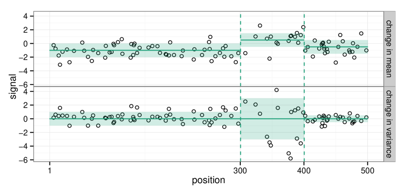
Figure 1: Two signals with the same breakpoints (vertical dashed lines) but different distributional changes. Black circles show $d=100$ sampled data points drawn from normal distributions defined on positions $\mathcal{P}=\{1,\dots,500\}$. Horizontal line segments and shaded bands show mean $\pm$ one standard deviation of the true normal distributions $D_{p}$. The goal of segmentation is to recover the distributions and/or breakpoints, using only the sampled data points.

1.2 Maximum likelihood segmentation algorithms

A segmentation algorithm takes the $d$ sampled data points as input, and returns a list of estimated distributions and/or breakpoints. In this section, we will review one class of segmentation algorithms called maximum likelihood segmentation.

A maximum likelihood segmentation model for multiple breakpoints in the mean of a normal distribution was proposed by Picard et al. (2005). Let $\mathbf{y}=\left[\begin{array}[]{ccc}y_{1}&\cdots&y_{d}\end{array}\right]^{\intercal}\in\mathbb{R}^{d}$ be the vector formed by the $d$ sampled data points, and let $\mathbf{p}=\left[\begin{array}[]{ccc}p_{1}&\cdots&p_{d}\end{array}\right]^{\intercal}\in\mathcal{P}^{d}$ be the corresponding vector of positions, ordered such that $p_{1}<\cdots<p_{d}$. Then for any number of segments $k\in\{1,\dots,d\}$, the estimated mean vector $\mathbf{\hat{y}}^{k}\in\mathbb{R}^{d}$ is defined as

$$\mathbf{\hat{y}}^{k}= \operatorname*{arg\,min}_{\mathbf{x}\in\mathbb{R}^{d}} ||\mathbf{y}-\mathbf{x}||^{2}_{2}$$ (1)

subject to $$k-1=\sum_{j=1}^{d-1}1_{x_{j}\neq x_{j+1}},$$

where $||\mathbf{x}||^{2}_{2}=\sum_{j=1}^{d}x_{j}^{2}$ is the squared $\ell_{2}$ norm. Note that the optimization objective of minimizing the squared error is equivalent to maximizing the Gaussian likelihood with uniform variance (Picard et al., 2005). For a fixed $k_{\text{max}}\leq d$, we can quickly calculate $\mathbf{\hat{y}}^{k}$ for all $k\in\{1,\dots,k_{\text{max}}\}$ using pruned dynamic programming (Rigaill, 2010). For any model size $k$, the estimated variance $\hat{\sigma}^{2}_{k}\in\mathbb{R}^{+}$ is defined as the mean of the squared residuals:

$$\hat{\sigma}_{k}^{2}=||\mathbf{y}-\mathbf{\hat{y}}^{k}||^{2}_{2}/d.$$ (2)

The derivation is similar for the model of multiple breakpoints in the variance of a normal distribution (Lavielle, 2005), and can be computed using the methods of Killick et al. (2012) or Cleynen et al. (2014). For both models, we visually represent the true distribution and estimates for $k\in\{2,\dots,5\}$ in Figure 2.

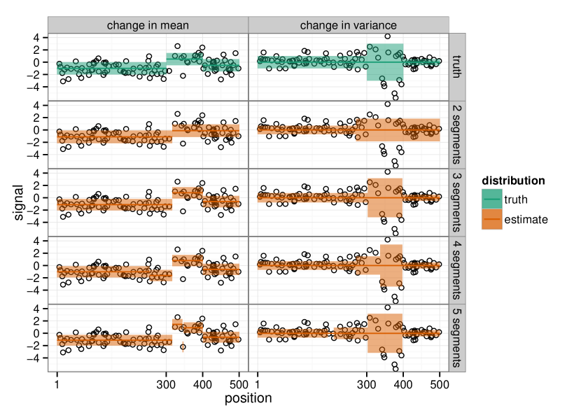
Figure 2: Comparing true and estimated distributions is one approach to segmentation model selection/evaluation but is not the subject of this paper. Top 2 panels: the same reference/true signals as in Figure 1. Others: estimated maximum likelihood models $\mathbf{\hat{y}}^{k},\hat{\sigma}^{2}_{k}$ for $k\in\{2,\dots,5\}$ segments.

1.3 Model selection

The segmentation model selection problem may be posed as follows. Of the 4 estimated segmentation models $k\in\{2,\dots,5\}$, which is the closest to the true model?

One method for segmentation model selection is to compare the true distribution with the estimated distributions (Figure 2), and choose the estimate whose distribution is closest to the true distribution. Assuming the true probability distributions $D_{p}$ are available, one could compare them with the estimates using a distance function such as the earth mover’s distance (Rubner et al., 1997), or some other distance function. However, the true distribution is not available in practice on real data, so in this paper we will not explore segmentation model selection via comparing distributions.

Instead, we propose a method for comparing the true and estimated breakpoints. For any $d$-vectors of data and positions $(\mathbf{x},\mathbf{p})$, we estimate the breakpoint locations using

$$\phi(\mathbf{x},\mathbf{p})=\big{\{}\lfloor(p_{j}+p_{j+1})/2\rfloor\text{ for all }j\in\{1,\dots,d-1\}\text{ such that }\mathbf{x}_{j}\neq\mathbf{x}_{j+1}\big{\}}.$$ (3)

Thus for any model size $k$, we estimate the breakpoint positions using $\phi(\mathbf{\hat{y}}^{k},\mathbf{p})$. In Figure 3, we compare these estimated breakpoints to the true set of breakpoints

$$B=\{j\in\mathbb{B}:D_{j}\neq D_{j+1}\}.$$ (4)

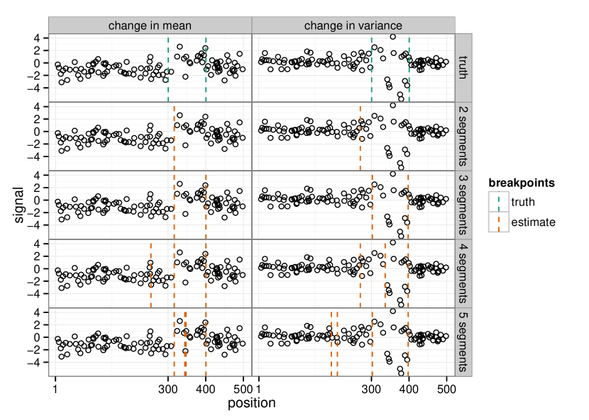
Figure 3: Same as Figure 2, but showing breakpoints instead of distributions. This paper proposes to compare the true and estimated breakpoints with the breakpointError function, which can be used for any reference/true distribution and any type of change.

Figure 3 clearly shows 3 distinct types of errors that are possible in estimating the breakpoint positions:

False negative (FN)

for both data sets, the models with 2 segments are suboptimal because they only detect 1 of the 2 true breakpoints.

False positive (FP)

for both data sets, the models with 4 segments are suboptimal since they detect 3 rather than 2 breakpoints. The models with 5 segments are even worse since they detect 4 breakpoints.

Imprecision (I)

of the two models with 3 segments, the breakpoints estimated for the change in variance data are more precise (closer to the true breakpoint positions).

This paper proposes the breakpointError function (Figure 4), which can be used to quantify these intuitive observations. The breakpointError can be computed to quantify how well a set of estimated breakpoint positions matches a true or reference set of breakpoints.

Figure 4: For the same data shown in Figure 3, we computed the breakpointError function (E) and its components. False positives (FP) occur when there are more estimated than true breakpoints, and false negatives (FN) are the opposite. For the correct model size (3 segments = 2 breakpoints), the imprecision function (I) quantifies the distance between the true and estimated breakpoint positions. The breakpointError is the sum of the other components (E=FP+FN+I).

2 Related Work

This paper has been revised and expanded from Chapter 4 of the doctoral thesis of Hocking (2012), which has not been previously published elsewhere. Differences include minor changes in notation, an expanded introduction, and more complete references.

The main subject of this paper is the breakpointError (defined in Section 3), which is a function for precisely measuring the breakpoint detection accuracy of a segmentation model. There are several other approaches for evaluating segmentation models. Levy-Leduc and Harchaoui (2008) compared the number of detected breakpoints with the number of true breakpoints, ignoring the positions of the breakpoints. A more precise method was proposed by Pierre-Jean et al. (2014), who checked if the detected breakpoints appear in regions of arbitrary size around the true breakpoints. In contrast, the breakpointError we propose in this paper has no arbitrary region size parameter. Bleakley and Vert (2011) used exact equality of the estimated and true breakpoint location in their asymptotic theoretical analysis. The breakpointError function is more precise since it is able to quantify that a guess close to a true breakpoint is better than a guess far from a true breakpoint. A final class of methods uses an annotated region database to quantify false positive and false negative breakpoint detections (Hocking et al., 2013; Rigaill et al., 2013). An annotation database can be created by drawing regions on scatterplots of the data using a graphical user interface (Hocking et al., 2014). Evaluating a segmentation model via annotated regions is similar to the breakpointError function we propose in this paper, and the precise link between these methods will be explored in Section 5.

Section 4 shows one example application of the breakpointError function, for determining the optimal form of penalty functions in segmentation models for simulated data. Many related penalties have been proposed for the change-point detection problem. The standard AIC or BIC criteria are not well adapted in this context since the model collection is exponential (Birgé and Massart, 2007; Schwarz, 1978; Akaike, 1973; Baraud et al., 2009), and also because change-points are discrete parameters (Zhang and Siegmund, 2007). Many criteria specifically adapted to change-point models have been proposed. For example, there are many different variants of the BIC (Yao, 1988; Lee, 1995; Zhang and Siegmund, 2007), and the model selection theory of Birgé and Massart suggest other penalties (Lavielle, 2005; Lebarbier, 2005; Birgé and Massart, 2007; Arlot and Massart, 2009). The precise differences between these penalties and the penalties that we find will be discussed in Section 4, but the main difference is that the penalties discussed in this paper are specifically designed to minimize the breakpointError (rather than some other function, e.g. the squared error or negative log likelihood of the data).

3 Definition of the breakpointError

Let us recall the notation of Section 1. Assume there are $P$ distinct positions in a series at which data could be gathered. Depending on the desired application, these positions could be indices in a data vector, genomic positions, or time points. Let $\mathcal{P}=\{1,\dots,P\}$ be the set of all such positions. For every position $p\in\mathcal{P}$, we assume there is some true probability distribution $D_{p}$. Let $\mathbb{B}=\{1,\dots,P-1\}$ be all bases after which a breakpoint is possible, and let $B=\{p\in\mathbb{B}:D_{p}\neq D_{p+1}\}$ be the set of true breakpoints.

The segmentation algorithm is given a sample of size $d\leq P$ of data $(p_{1},y_{1}),\dots,(p_{d},y_{d})$, with positions $p_{i}\in\mathcal{P}$ and noisy observations $y_{i}\sim D_{p_{i}}$ for all samples $i\in\{1,\dots,d\}$. The job of the segmentation algorithm is to return a breakpoint guess $G\subseteq\mathbb{B}$. The object of this section is to define the breakpointError $E^{B}_{\text{exact}}(G)$, which quantifies the accuracy of the guess $G$ with respect to the true breakpoints $B$.

3.1 Desired properties of the breakpointError function

We would like the breakpointError function $E^{B}_{\text{exact}}:2^{\mathbb{B}}\rightarrow\mathbb{R}^{+}$ to satisfy the following properties:

• (correctness) Guessing exactly right costs nothing: $E^{B}_{\text{exact}}(B)=0$.

• (precision) A guess closer to a real breakpoint is less costly:
  if $B=\{b\}$ and $0\leq i<j$, then $E^{B}_{\text{exact}}(\{b+i\})\leq E^{B}_{\text{exact}}(\{b+j\})$ and $E^{B}_{\text{exact}}(\{b-i\})\leq E^{B}_{\text{exact}}(\{b-j\})$.

• (FP) False positive breakpoints are bad: if $b\in B$ and $g\not\in B$, then $E^{B}_{\text{exact}}(\{b\})<E^{B}_{\text{exact}}(\{b,g\})$.

• (FN) Undiscovered breakpoints are bad: $b\in B\Rightarrow E^{B}_{\text{exact}}(\{b\})<E^{B}_{\text{exact}}(\emptyset)$.

In the next section we define the breakpointError, which satisfies all 4 properties.

3.2 Definition of the breakpointError function

In this section, we use the exact breakpoint locations $B=\{B_{1},\dots,B_{n}\}$ to define the breakpointError function.

We define the error of a breakpoint location guess $g\in\mathbb{B}$ as a function of the closest breakpoint in $B$. So first we put the breaks in order, by writing them as $B_{1}<\cdots<B_{n}$. Then, we define a set of intervals $R_{B}=\{\mathbf{r}_{1},\dots,\mathbf{r}_{n}\}$ that form a partition of $\mathbb{B}$. For each breakpoint $B_{i}$ we define the region ${\mathbf{r}}_{i}=[\underline{r}_{i},\overline{r}_{i}]\in\mathbb{I}\mathbb{B}$, where $\mathbb{I}\mathbb{B}\subset 2^{\mathbb{B}}$ denotes the set of all intervals of $\mathbb{B}$. We take the notation conventions from the interval analysis literature (Nakao et al., 2010).

We define the upper limit of region $i$ as

$$\overline{r}_{i}=\begin{cases}P-1&\text{if }i=n\\ \lfloor(B_{i+1}+B_{i})/2\rfloor&\text{otherwise}\end{cases}$$ (5)

and the lower limit as

$$\underline{r}_{i}=\begin{cases}1&\text{if }i=1\\ \overline{r}_{i-1}+1&\text{otherwise}.\end{cases}$$ (6)

The breakpoints $B_{i}$ and regions $\mathbf{r}_{i}$ are labeled for a small signal in Figure 5.

Figure 5: For a small signal with 2 breakpoints, and for breakpoints $i\in\{1,2\}$, we plot the $\ell_{i}$ functions that measure the precision of a guess in $\mathbf{r}_{i}=[\underline{r}_{i},\overline{r}_{i}]$. The blue signal $\mathbf{m}\in\mathbb{R}^{22}$ has 2 breakpoints: $B=\{4,14\}$. To emphasize the discrete nature of the data, N is drawn at each of the $P=22$ distinct positions at which data could be gathered.

Intuitively, if we observe a breakpoint guess $g\in\mathbf{r}_{i}$, then its closest breakpoint is $B_{i}$. To define the best guess in each region, we use piecewise affine functions $C_{\underline{r},b,\overline{r}}:\mathbb{R}\rightarrow[0,1]$ defined as follows:

$$C_{\underline{r},b,\overline{r}}(g)=\begin{cases}0&\text{if }g=b\\ (b-g)/(x-\underline{r})&\text{if }\underline{r}<g<b\\ (g-b)/(\overline{r}-x)&\text{if }b<g<\overline{r}\\ 1&\text{ otherwise}.\end{cases}$$ (7)

For each breakpoint $i$ we measure the precision of a guess $g\in\mathbb{B}$ using

$$\ell_{i}(g)=C_{\underline{r}_{i},B_{i},\overline{r}_{i}}(g).$$ (8)

These piecewise affine functions are shown in Figure 5 for a small signal with 2 breakpoints. Note that there is some degree of arbitrary choice in the definition of the $\ell_{i}$ functions. For example, properly defined piecewise quadratic functions could also satisfy the precision property desired of the breakpointError (Section 3.1).

Now, we are ready to define the exact breakpointError of a set of guesses $G\subseteq\mathbb{B}$. First, let $G\cap\mathbf{r}$ be the subset of guesses $G$ that fall in region $\mathbf{r}$.

Then, we define the false negative rate for region $\mathbf{r}$ as

$$\text{FN}(G,\mathbf{r})=\begin{cases}1&\text{if }G\cap\mathbf{r}=\emptyset\\ 0&\text{otherwise}\end{cases}$$ (9)

and the false positive rate for region $\mathbf{r}$ as

$$\text{FP}(G,\mathbf{r})=\begin{cases}0&\text{if }G\cap\mathbf{r}=\emptyset\\ |G\cap\mathbf{r}|-1&\text{otherwise}\end{cases}$$ (10)

and the imprecision of the best guess in region $r$ as

$$I(G,\mathbf{r},\ell)=\begin{cases}0&\text{if }G\cap\mathbf{r}=\emptyset\\ \min_{g\in G\cap\mathbf{r}}\ell(g)&\text{otherwise}.\end{cases}$$ (11)

When there are no breakpoints, we have $B=\emptyset$ and $R_{B}=\emptyset$. But we still would like to quantify the false positives, so let $G\setminus\big{(}\cup R_{B}\big{)}$ be the set of guesses $G$ outside of the breakpoint regions $R_{B}$.

Definition 2.

The breakpointError of set of breakpoint guesses $G$ with respect to the true breakpoints $B$ is the sum of the False Positive, False Negative, and Imprecision functions:

$${E}_{\text{exact}}^{B}(G)=\big{|}G\setminus(\cup R_{B})\big{|}+\sum_{i=1}^{|B|}\textrm{FP}(G,\mathbf{r}_{i})+\textrm{FN}(G,\mathbf{r}_{i})+I(G,\mathbf{r}_{i},\ell_{i}).$$

3.3 Implementation

To compute the exact breakpointError, we first sort lists of $n=|B|$ and $m=|G|$ items. Using the quicksort algorithm, this requires $O(n\log n+m\log m)$ operations in the average case (Cormen et al., 1990). Once sorted, the components of the cost can be computed in linear time $O(n+m)$. So, overall the computation of the error can be accomplished in best case $O(n+m)$, average case $O(n\log n+m\log m)$ operations. Its computation is implemented in efficient C code in the breakpointError R package on R-Forge, which can be installed in R using

install.packages("breakpointError", repos="http://r-forge.r-project.org")

4 Penalties with minimal breakpointError in simulations

In this section, we show several examples of how to use the breakpointError function to determine penalties which minimize the train and test breakpointError in simulated data sets. In all cases, we will assume that there is a database of several piecewise constant signals with Gaussian noise. The goal is to learn a penalty constant that can be shared between signals with different properties. In each of the following sections, we will first present an empirical analysis of several simulated signals using the breakpointError. Then, we will discuss the relationship of our results to relevant theoretical results.

4.1 Sampling density normalization

The first problem we consider is finding a penalty that is invariant to sampling density. This is important because sampling density is often not uniform in real data sets. In fact, we see a sampling density between 40 and 4400 kilobases per probe in the neuroblastoma data set of Hocking et al. (2013). We would like to construct a single algorithm or penalty function that can be used for each of these segmentation problems.

So to determine the form of the penalty function that can best adapt to this variation, we analyze the following simulation. We create a true piecewise constant signal $\mathbf{m}\in\mathbb{R}^{P}$ over $P=70000$ base pairs, with breakpoints every 10000 base pairs, shown as the blue line in Figure 6. Then, we define a signal sample size $d_{i}\in\{70,\dots,70000\}$ for every noisy signal $i\in\{1,\dots,z\}$. Let $y_{i}\in\mathbb{R}^{d_{i}}$ be noisy signal $i$, sampled at positions $p_{i}\in\mathcal{P}^{d_{i}}$, with $p_{i1}<\cdots<p_{i,d_{i}}$. We sample every probe $j$ from the $y_{ij}\sim N(m_{p_{ij}},1)$ distribution. These samples are shown as the black points in Figure 6.

We would like to learn some model complexity parameter $\lambda$ on the first noisy signal, and use it for accurate breakpoint detection on the second noisy signal. In other words, we are looking for a model selection criterion which is invariant to sampling density.

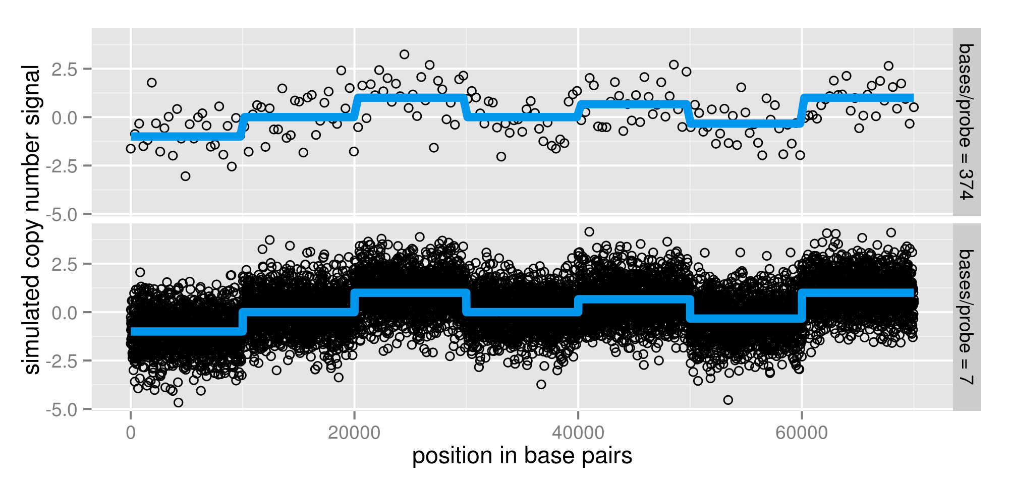
Figure 6: Two noisy signals (black) sampled from a true piecewise constant signal (blue). Note that these are the same signals that appear in Figure 19.

To attack this problem, we proceed as follows. For every signal $i$, we use pruned dynamic programming to calculate the maximum likelihood estimator $\mathbf{\hat{y}}^{k}_{i}\in\mathbb{R}^{d_{i}}$ (1), for several model sizes $k\in\{1,\dots,k_{\text{max}}\}$ (Rigaill, 2010). Then, we define the model selection criteria

$$k^{\alpha}_{i}(\lambda)=\operatorname*{arg\,min}_{k}\lambda kd_{i}^{\alpha}+||\mathbf{y_{i}}-\mathbf{\hat{y}}^{k}_{i}||_{2}^{2}.$$ (12)

Each of these is a function $k_{i}^{\alpha}:\mathbb{R}^{+}\rightarrow\{1,\dots,k_{\text{max}}\}$ that takes a model complexity tradeoff parameter $\lambda$ and returns the optimal number of segments for signal $i$. The goal is to find a penalty exponent $\alpha\in\mathbb{R}$ that lets us generalize $\lambda$ between different signals $i$.

To quantify the accuracy of a segmentation for signal $i$, let $\text{BErr}_{i}(k)$ be the breakpointError of the model with $k$ segments. This is a function $\text{BErr}_{i}:\{1,\dots,k_{\text{max}}\}\rightarrow\mathbb{R}^{+}$, defined as

$$\text{BErr}_{i}(k)=E_{\text{exact}}^{B}\left[\phi(\mathbf{\hat{y}}_{i}^{k},p_{i})\right].$$ (13)

where $B$ is the set of real breakpoints in the true piecewise constant signal $\mathbf{m}$.

In Figure 7, we plot $\text{BErr}_{i}$ for the 2 simulated signals $i$ shown previously. As expected, the model recovers more accurate breakpoints from the signal sampled at a higher density.

Figure 7: Exact breakpoint error $\text{BErr}_{i}(k)$ for two signals $i$ and several model sizes $k$. Note that these are the same error curves that appear in the Breakpoint panels of Figure 20.

Now, let us define the penalized model breakpoint error $E^{\alpha}_{i}:\mathbb{R}^{+}\rightarrow\mathbb{R}^{+}$ as

$$E^{\alpha}_{i}(\lambda)=\text{BErr}_{i}\left[k^{\alpha}_{i}(\lambda)\right].$$ (14)

In Figure 8, we plot these functions for the two signals $i$ shown previously, and for several penalty exponents $\alpha$.

The dots in Figure 8 show the optimal $\lambda$ found by minimizing the penalized model breakpoint detection error:

$$\hat{\lambda}^{\alpha}_{i}=\operatorname*{arg\,min}_{\lambda\in\mathbb{R}^{+}}E^{\alpha}_{i}(\lambda)$$ (15)

Figure 8 suggests that $\alpha\approx 1/2$ defines a penalty with aligned error curves, which will result in $\hat{\lambda}_{i}^{\alpha}$ values that can be generalized between profiles.

Figure 8: Model selection error curves $E_{i}^{\alpha}(\lambda)$ for 2 signals $i$ and several exponents $\alpha$. The penalty contains a term for the number of points sampled $d_{i}^{\alpha}$.

Now, we are ready to define 2 quantities that will be able to help us choose an optimal penalty exponent $\alpha$.

First, let us consider the training error over the entire database:

$$E^{\alpha}(\lambda)=\sum_{i=1}^{z}E_{i}^{\alpha}(\lambda),$$ (16)

and we define the minimal value of this function as

$$E^{*}(\alpha)=\min_{\lambda}E^{\alpha}(\lambda).$$ (17)

In Figure 9, we plot these training error functions $E^{\alpha}$ and their minimal values $E^{*}$ for several values of $\alpha$. It is clear that the minimum training error is found for some penalty exponent $\alpha$ near 1/2, and we would like to find the precise $\alpha$ that results in the lowest possible minimum $E^{*}(\alpha)$.

Figure 9: Training error functions $E^{\alpha}$ in black and their minimal values $E^{*}(\alpha)$ in red. The penalty contains a term for the number of points sampled $d_{i}^{\alpha}$.

We also consider the test error over all pairs of signals when training on one and testing on another:

$$\text{TestErr}(\alpha)=\sum_{i\neq j}E^{\alpha}_{i}(\hat{\lambda}_{j}^{\alpha}).$$ (18)

In Figure 10, we plot $E^{*}$ and TestErr for a grid of $\alpha$ values. It is clear that the optimal penalty is given by $\alpha=1/2$. This corresponds to the following model selection criterion which is invariant to the number of data points sampled $d_{i}$ (for different simulated signals $i$ with the same true breakpoints):

$$k_{i}(\lambda)=\operatorname*{arg\,min}_{k}\lambda k\sqrt{d_{i}}+||\mathbf{y}_{i}-\mathbf{\hat{y}}_{i}^{k}||^{2}_{2}$$ (19)

Figure 10: Train and test breakpoint detection error as a function of penalty exponent $\alpha$. The penalty contains a term for the number of points sampled $d_{i}^{\alpha}$. Mean error is drawn as a black line, with one standard deviation shown as a grey band.

As explained by Arlot and Celisse (2010), a model selection procedure can be either efficient or consistent. An efficient procedure for model estimation accurately recovers the true piecewise constant signal, whereas a consistent procedure for model identification accurately recovers the breakpoints. Since we attempt to minimize the breakpointError, we are attempting to construct a consistent penalty, not an efficient penalty.

In general terms, the fact that we find a nonzero exponent $\alpha$ for our $d_{i}^{\alpha}$ penalty term agrees with other results. In particular, Arlot (2008) proposed an optimal procedure to select model complexity parameters in cross-validation by normalizing by the sample size $d_{i}$.

The $\sqrt{d_{i}}$ term that we find here using simulations is in agreement with Fischer (2011), who used finite sample model selection theory to find a $\sqrt{d_{i}}$ term in a penalty optimal for clustering.

When theoretically deriving an efficient penalty for segmentation model estimation in the non-asymptotic setting, Lebarbier (2005) obtained a $\log d_{i}$ term. This contrasts our result, which attempts to find a consistent penalty, and uses the breakpointError to find a $\sqrt{d_{i}}$ penalty term. But in fact this is in agreement with classical results that the efficient AIC underpenalizes with respect to the consistent BIC, as shown in Table 1.

Efficient	Penalty	Consistent	Penalty
Model	Term	Model	Term
AIC	2	BIC	$\log d_{i}$
Lebarbier	$\log d_{i}$	This work	$\sqrt{d_{i}}$

Table 1: Comparing our results with Lebarbier, in the context of classical results involving AIC and BIC. The BIC is designed for model identification and penalizes more than the AIC. Likewise, our penalty examines model identification using the breakpoint detection error, and penalizes more than the efficient penalty proposed by Lebarbier.

4.2 Signal length normalization

In real array CGH data, we need to analyze chromosomes of varying length in base pairs. For example, human chromosome 1 is the largest at about 250 mega base pairs, and chromosome 22 is the smallest with only about 36 mega base pairs. But we expect that the number of breakpoints is proportional to the length of the chromosome in base pairs, and we would like to design a model selection criterion that is invariant to the signal length.

So as a first step toward constructing a penalty that is invariant to the number of breakpoints, we consider the following simulation where we fix the number of points sampled at $d_{i}=2000$, and vary the length of the signal sampled. In Figure 11, we show samples of 2 different lengths $l_{i}$, for the same true piecewise constant signal $\mathbf{m}$. This simulation is somewhat unrealistic since the number of data points $d_{i}$ in real data sets is usually proportional to the signal length $l_{i}$. We will consider a more realistic simulation model and a more complicated penalty in the next section.

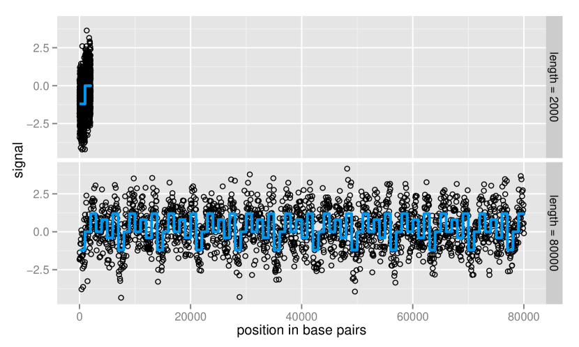
Figure 11: Samples of 2 different lengths $l_{i}$ but constant number of points $d=2000$.

For each signal $i$, we define the penalty

$$k_{i}^{\beta}(\lambda)=\operatorname*{arg\,min}_{k}\lambda kl_{i}^{\beta}+||\mathbf{y}_{i}-\mathbf{\hat{y}}_{i}^{k}||^{2}_{2},$$ (20)

where $l_{i}$ is the length of the signal in base pairs. The goal will be to find a $\beta$ that can be used for signals of varying length.

In Figure 12, we show the breakpoint detection error curves for two signals and several penalty exponents $\beta$. These curves seem to align when $\beta=-1/2$.

Figure 12: Breakpoint detection error curves for several penalty exponents $\beta$ and 2 samples of varying length in base pairs $l_{i}$. The penalty contains a term $l_{i}^{\beta}$.

In Figure 13, we plot the train and test error curves over the entire set of simulated signals. These curves indicate minimal breakpoint detection error at $\beta=-1/2$, corresponding to the following penalty:

$$k_{i}(\lambda)=\operatorname*{arg\,min}_{k}\frac{\lambda k}{\sqrt{l_{i}}}+||\mathbf{y}_{i}-\mathbf{\hat{y}}_{i}^{k}||^{2}_{2}.$$ (21)

Figure 13: Train and test error curves for signals of different length in base pairs $l_{i}$. The penalty contains a term $l_{i}^{\beta}$.

Interestingly, the $1/\sqrt{l_{i}}$ term that we obtain here is in good agreement with our previous result that the optimal penalty for variable sampling density $d_{i}$ should have a $\sqrt{d_{i}}$ term. In particular, we can re-parameterize the problem to be in terms of the number of points sampled per segment $\rho_{i}=d_{i}/k_{i}$. In Section 4.1 we held $k_{i}$ constant but in this section we hold $d_{i}$ constant. In both cases we have a penalty with a $\sqrt{\rho_{i}}=\sqrt{d_{i}/k_{i}}$ term.

However, we do not know the number of segments $k_{i}$ in advance. But we supposed that the number of segments is proportional to the number of base pairs $l_{i}$, so we can use that in the penalty. This suggests a penalty that takes the form of $\sqrt{d_{i}/l_{i}}$. So in the next section, we confirm that this intuition works for constructing an optimal penalty.

4.3 Combining normalizations

In this section, we show that we can combine the results of the previous sections to create composite invariant penalties. In particular, to normalize for sampling density $d_{i}$ and length in base pairs $l_{i}$, we need $\sqrt{d_{i}}$ and $1/\sqrt{l_{i}}$ terms in the penalty, respectively. This suggests that when considering variable $d_{i}$ and $l_{i}$, we need a $\sqrt{d_{i}/l_{i}}$ term in the penalty, and in this section we show that this intuitive construction results in an optimal penalty.

In Figure 14, we plot 2 signals with different number of points $d_{i}$ and length in base pairs $l_{i}$. In particular we tested $d_{i}\in\{50,\dots,1000\}$ and $l_{i}\in\{200,\dots,1000\}$. We would like to find a penalty that allows us to generalize model complexity tradeoff parameters $\lambda$ between these signals.

For each signal $i$, we define the penalty

$$k_{i}^{\alpha,\beta}(\lambda)=\operatorname*{arg\,min}_{k}\lambda k{d_{i}}^{\alpha}l_{i}^{\beta}+||\mathbf{y}_{i}-\mathbf{\hat{y}}_{i}^{k}||^{2}_{2},$$ (22)

where $l_{i}$ is the signal length in base pairs and $d_{i}$ is the number of points sampled. We will attempt to determine a pair of $\alpha$ and $\beta$ values that allow accurate breakpoint detection in signals of varying length and number of points sampled. Based on the results in Sections 4.1 and 4.2, we expect to find $\alpha=1/2$ and $\beta=-1/2$.

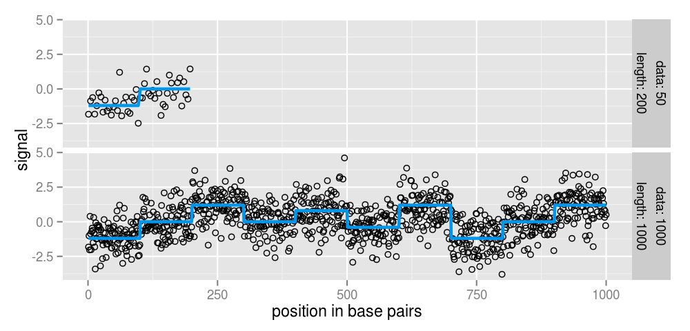
Figure 14: Two signals with a different number of points $d_{i}$ and length in base pairs $l_{i}$.

In Figure 15, we plot the train and test breakpoint error functions as a function of both $\alpha$ and $\beta$. It is clear that the minimum is achieved by penalties near $\alpha=1/2,\beta=-1/2$, which corresponds to a penalty of

$$k_{i}^{\alpha,\beta}(\lambda)=\operatorname*{arg\,min}_{k}\lambda k\sqrt{d_{i}/l_{i}}+||\mathbf{y}_{i}-\mathbf{\hat{y}}_{i}^{k}||^{2}_{2},$$ (23)

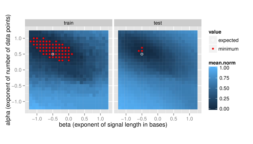
Figure 15: Train and test error functions for several signals of varying number of points $d_{i}$ and length $l_{i}$. The penalty contains a term $d_{i}^{\alpha}l_{i}^{\beta}$. Mean error values normalized to $[0,1]$, minimum values indicated in red, and expected value $\alpha=1/2,\beta=-1/2$ in white.

4.4 Optimal penalties for the fused lasso signal approximator

In the previous sections, we used theoretical arguments and simulation experiments to determine the optimal penalties for maximum likelihood segmentation (1). In this section, we demonstrate that the same approach can be used to find optimal penalties for another model, the Fused Lasso Signal Approximator (FLSA).

We used the flsa function in version 1.03 of the flsa package from CRAN to calculate the FLSA (Hoefling, 2009). Let $\mathbf{x}\in\mathbb{R}^{d}$ be the noisy copy number signal for one chromosome. The FLSA solves the following optimization problem:

$$\operatorname*{arg\,min}_{\mathbf{m}\in\mathbb{R}^{d}}\frac{1}{2}\sum_{j=1}^{d}(x_{j}-m_{j})^{2}+\lambda_{1}\sum_{j=1}^{d}|m_{j}|+\lambda_{2}\sum_{j=1}^{d-1}|m_{j}-m_{j+1}|.$$ (24)

First, we take $\lambda_{1}=0$ since we are concerned with breakpoint detection, not signal sparsity. In this section, our aim is to determine a parameterization for $\lambda_{2}$ that we will be able to find similar breakpoints in signals of varying sampling density.

We use the same setup that we used to determine optimal penalties for maximum likelihood segmentation, as described in Section 4.1 and shown again in Figure 16.

Figure 16: Simulated signals with different sampling density.

In particular, for every signal $i\in\{1,\dots,z\}$, let $\mathbf{y}_{i}\in\mathbb{R}^{d_{i}}$ be the noisy data, sampled at positions $\mathbf{p}_{i}\in\mathcal{P}^{d_{i}}$. To find an optimal penalty for these data, first let $\lambda_{2}=\lambda d_{i}^{\alpha}$. For each signal $i$, exponent $\alpha\in\mathbb{R}$, and tradeoff parameter $\lambda\in\mathbb{R}^{+}$, we define the optimal smoothing as

$$\mathbf{\hat{y}}^{\lambda,\alpha}_{i}=\operatorname*{arg\,min}_{\mathbf{m}\in\mathbb{R}^{d_{i}}}\frac{1}{2}||\mathbf{y}_{i}-\mathbf{m}||_{2}^{2}+\lambda d_{i}^{\alpha}\sum_{j=1}^{d_{i}-1}|m_{j}-m_{j+1}|.$$ (25)

Then, we define the breakpoint detection error as a function of the breaks in the smoothed signal:

$$E_{i}^{\alpha}(\lambda)=E^{B}_{\text{exact}}\left[\phi\left(\mathbf{\hat{y}}^{\lambda,\alpha}_{i},\mathbf{p}_{i}\right)\right],$$ (26)

where the breakpoint function $\phi$ is defined in (3).

We plot $E_{i}^{\alpha}$ for 2 signals $i$ and several penalty exponents $\alpha$ in Figure 17. Note that the functions appear to align when $\alpha=1$.

Figure 17: Model complexity breakpoint error functions $E_{i}^{\alpha}$.

To evaluate which penalty parameter $\alpha$ results in optimal fitting and learning, we computed train error $E^{*}$ and TestErr as defined in (16) and (18). These functions are plotted in Figure 18, and suggest that a value of $\alpha=1$ is optimal. This analysis suggests that taking $\lambda_{2}=\lambda d_{i}$ is optimal for breakpoint detection using FLSA. This agrees with the observation of Hocking et al. (2013) that the flsa.norm penalty with a $d_{i}$ term works better than the un-normalized flsa penalty.

However, we obtained a different penalty ($\alpha=0.5$) in Section 4.1 for another model, maximum likelihood segmentation. These differences in optimal $\alpha$ values are due to the differences in how model complexity is measured in the two models. Maximum likelihood segmentation measures model complexity using the $\ell_{0}$ pseudo-norm of the difference vector of $\mathbf{m}$, whereas the FLSA uses the $\ell_{1}$-norm.

We conclude by noting that this procedure could also be applied to find penalties for FLSA that depend on other signal properties such as length in base pairs $l_{i}$. However, we did not pursue this since FLSA does not work as well as maximum likelihood segmentation in practice on real data (Hocking et al., 2013).

Figure 18: Train and test error as a function of penalty exponent $\alpha$. The penalty has a term for the number of points sampled $d_{i}^{\alpha}$.

4.5 Applying the penalties to real data

In Sections 4.1-4.2, we found penalties with minimum breakpointError for simulated data with varying number of data points sampled $d_{i}$ and length $l_{i}$ in base positions (with $l_{i}$ proportional to the number of breakpoints). In Section 4.3, we demonstrated that these results can be combined. We also found that the optimal penalty should include a term for the estimated variance $\hat{s}_{i}^{2}$ (Hocking, 2012). These results suggested the following penalty, for every signal $i$:

$$k_{i}(\lambda)=\operatorname*{arg\,min}_{k}\lambda k\hat{s}_{i}^{2}\sqrt{d_{i}/l_{i}}+||\mathbf{y}_{i}-\mathbf{\hat{y}}_{i}^{k}||^{2}_{2}$$ (27)

In Table 2, we report results of using the suggested penalties on the neuroblastoma data set described by Hocking et al. (2013). The cghseg.k penalty which was found to be the best by Hocking et al. (2013) has a term for number of data points sampled $d_{i}$ (no square root) but no terms for length $l_{i}$ nor estimated variance $\hat{s}_{i}$. The penalty terms suggested in this section do not improve breakpoint detection error in the neuroblastoma data set. This observation suggests that distribution that generates the real data is more complex than the simple simulation model considered in this paper.

	points	length	variance	train	test.mean	test.sd
cghseg.k	1	0	0	2.19	2.20	1.01
cghseg.k.var	1	0	2	2.46	2.73	1.98
cghseg.k.sqrt.d	$1/2$	0	0	3.51	3.87	1.58
cghseg.k.sqrt	$1/2$	$-1/2$	0	4.30	6.11	5.02
cghseg.k.sqrt.d.var	$1/2$	0	2	3.19	4.47	5.02
cghseg.k.sqrt.var	$1/2$	$-1/2$	2	4.18	6.38	7.61

Table 2: Breakpoint detection error of several penalties on the neuroblastoma data set, with 1 row for each penalty. The exponent of the number of data points $d_{i}$, length $l_{i}$, and variance $\hat{s}_{i}$ terms in the penalty is shown with the train and test annotation error (percent incorrect regions).

Practically speaking, we still would like to find a penalty with optimal breakpoint detection for any particular real data set such as the neuroblastoma data. Rigaill et al. (2013) achieved state-of-the-art breakpoint detection in the neuroblastoma data set by learning the penalty constants using a training data set of manually annotated regions. For the rest of this paper, we will discuss the relationship of the breakpointError to these annotation-guided methods.

5 Annotation error functions for real data sets

In this section, we define several annotation error functions which can be used in real data sets (Table 3). In real data, we do not have access to the true piecewise constant signal $\mathbf{m}$, nor the underlying set of breakpoints $B$. So the breakpointError defined in the Section 3 is not readily computable. We will first show how in real data, we can compute another function called the incomplete annotation error. Then, we will demonstrate its relationship to the breakpointError using the complete annotation error function.

Section	Error function	Symbol	Need	counts incorrect
3.2	breakpointError	$E^{B}_{\text{exact}}$	true breakpoints $B$	guesses
5.1	incomplete annotation error	$E_{\text{incomplete}}^{A}$	some annotations $A$	guesses
5.2	complete annotation error	$E_{\text{complete}}^{A}$	all breakpoint annotations $A$	guesses
5.3	01 annotation error	$E_{01}^{A}$	some annotations $A$	regions

Table 3: Several breakpoint detection error functions, and how much prior knowledge is needed to compute each. The breakpointError needs the most prior knowledge and can only be used in simulations when the true breakpoints $B$ are known. In contrast, the incomplete/01 annotation error can be used in real data sets by using visual inspection of scatterplots to create annotations $A$.

5.1 Incomplete annotation error for real data

By plotting a real data set, we can easily identify regions that contain breakpoints by visual inspection, as shown in Figure 19.

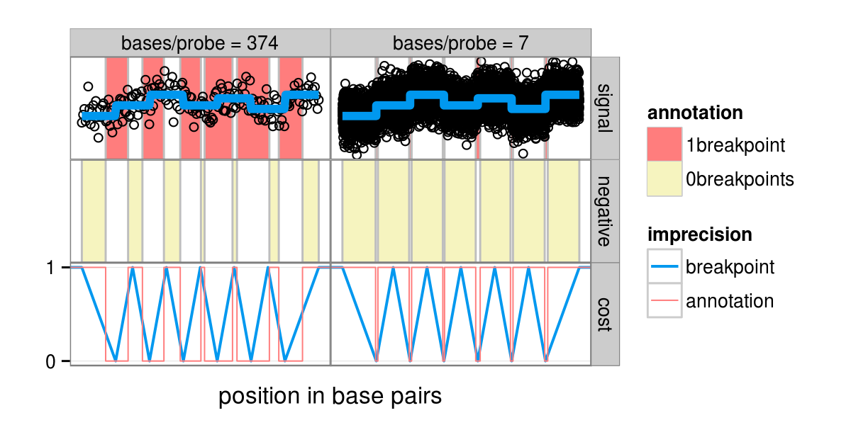
Figure 19: Top: simulated noisy signals (black) with their true piecewise constant signals $\mathbf{m}$ (blue) and visually-determined breakpoint annotations $A$ (red). Middle: negative annotations $A^{0}$ constructed using (31). Bottom: breakpoint detection imprecision curves for the breakpointError $\ell_{i}$ (11) and the annotation error $\hat{\ell}_{i}$ (33).

Recall that there are $P$ distinct positions in a series at which data could be gathered, and that $\mathbb{B}=\{1,\dots,P-1\}$ is the set of all positions after which a breakpoint is possible.

Definition 3.

A set of $n$ annotations can be written as $A=\{(a_{1},\mathbf{r}_{1}),\dots,(a_{n},\mathbf{r}_{n})\}$. For each annotation $i$, $\mathbf{r}_{i}\subset\mathbb{I}\mathbb{B}$ is an interval that defines the region, and $a_{i}\subseteq\{0,1,\dots\}$ is an interval of allowable breakpoint counts in this region.

For example, consider the annotated regions in Table 4.

$i$	Allowed breakpoints $a_{i}$	Region $\mathbf{r}_{i}$
1	{0}	[5,10]
2	{1}	[20,30]
3	{1,2,…}	[40,70]
4	{0}	[80,100]

Table 4: Sample annotated regions for a signal sampled on $P=100$ base pairs. An annotation $a_{i}$ indicates how many breakpoints are allowed in the corresponding region $\mathbf{r}_{i}$. There are 0 breaks in bases 5-10 and 80-100. There is exactly 1 break in bases 20-30. There is at least 1 break in bases 40-70.

Given a set of breakpoint guesses $G\subseteq\mathbb{B}$, we define the annotation-dependent false positive count as

$$\hat{\text{FP}}(G,\mathbf{r},a)=\big{(}|G\cap\mathbf{r}|-\max(a)\big{)}_{+}$$ (28)

where the positive part function is defined as

$$x_{+}=\begin{cases}x&\text{ if }x>0\\ 0&\text{ otherwise.}\end{cases}$$ (29)

Similarly, the annotation-dependent false negative count is defined as

$$\hat{\text{FN}}(G,\mathbf{r},a)=\big{(}\min(a)-|G\cap\mathbf{r}|\big{)}_{+}.$$ (30)

Definition 4.

Let $A$ be a set of annotations and $G\subseteq\mathbb{B}$ a set of breakpoint guesses. The incomplete annotation error is the count of annotation-dependent false positives and false negatives:

$$E^{A}_{\text{incomplete}}(G)=\sum_{i=1}^{n}\hat{\textrm{FP}}(G,\mathbf{r}_{i},a_{i})+\hat{\textrm{FN}}(G,\mathbf{r}_{i},a_{i}).$$

In the case of analyzing the simulated signals in the top panels of Figure 19, let us consider the set of 6 annotations $\hat{A}=\{(\hat{a}_{1},\hat{\mathbf{r}}_{1}),\dots,(\hat{a}_{6},\hat{\mathbf{r}}_{6})\}$ depicted using the red rectangles. These rectangles were determined by visual inspection of the scatterplots. I used the SegAnnDB interactive annotation web site to view the data and save a database of 6 regions per profile (Hocking et al., 2014). Every region $\hat{\mathbf{r}}_{i}$ contains exactly 1 breakpoint, so we have $\hat{a}_{i}=\{1\}$ for every annotation $i\in\{1,\dots,6\}$. In real data we will probably only be able to see a subset of the real breakpoints, but we analyze the complete set of breakpoints in these simulated data to illustrate the approximation induced by the annotation process.

Given any set of non-intersecting annotations $A$, we can write $\underline{r}_{1}<\cdots<\underline{r}_{n}$ to order the regions. Then we can define $|A|+1$ negative annotations as

$$A^{0}=\big{\{}(0,[1,\underline{r}_{1}-1]),\ (0,[\overline{r}_{1}+1,\underline{r}_{2}-1]),\ \dots,\ (0,[\overline{r}_{n-1}+1,\underline{r}_{n}-1]),\ (0,[\underline{r}_{n}+1,d-1])\big{\}},$$ (31)

as drawn with yellow rectangles in the middle panels of Figure 19. We will use the complete set of annotations $\hat{A}\cup\hat{A}^{0}$ to define the annotation error $E^{\hat{A}\cup\hat{A}^{0}}_{\text{incomplete}}(G)$ for breakpoint guesses $G$ given by models of these simulated signals.

In Figure 20, we plot some model selection error functions for the 2 simulated signals shown in Figure 19. It is clear that the annotation error is a good approximation of the breakpointError, and there are several interesting observations to note.

• Signal: in these simulated data, the true piecewise constant signal $\mathbf{m}$ is available, so an efficient model selection procedure (Arlot and Celisse, 2010) would select the estimated model which is closest to the true signal. That idea is illustrated in Figure 2, and can be used in this context by minimizing

  $$E_{\text{signal}}(k)=\log_{10}\left[\frac{1}{d}\sum_{i=1}^{d}(\mathbf{\hat{y}}_{i}^{k}-\mathbf{m}_{i})^{2}\right].$$ (32)

  • In Figure 20, for the signal sampled at 7 bases/probe, the minimum of the Signal error identifies a model with 7 segments.

  • For the signal sampled at 374 bases/probe, the minimum of the error identifies a model with only 5 segments.

• Breakpoint: in these simulated data, the true breakpoints $B$ are available, so we can compute and minimize the breakpointError as a consistent model selection procedure (Arlot and Celisse, 2010). For both signals, the minimum of the breakpointError identifies a model with 7 segments (6 breakpoints).

• Annotation: we use a set of annotated regions to compute the incomplete annotation error, which also identifies a model with 7 segments. It is clear that the annotation error is a good approximation of the breakpointError. In the next section, we explicitly demonstrate the link between the breakpointError and the annotation error.

Figure 20: Model selection error curves for 2 simulated signals. Minima are highlighted using circles.
Signal: the log squared error $E_{\text{signal}}$ of the estimated signal with respect to the true piecewise constant signal (see text).
Breakpoint: exact breakpointError $E^{B}_{\text{exact}}$.
Annotation: incomplete annotation error $E^{\hat{A}\cup\hat{A}^{0}}_{\text{incomplete}}$.

5.2 Link with breakpointError using complete annotation error

It is clear from Figure 20 that the annotation error is a good approximation of the exact breakpoint error when the annotations $A$ agree with the real breakpoints $B$. In this section, we make this intuition precise by showing exactly how to relax the breakpointError to obtain the annotation error. There are two steps:

1. We define the complete annotation error by relaxing the definition of the exact breakpointError.

2. We show that the complete annotation error is equivalent to the incomplete annotation error when we have a complete set of annotations.

We will define the complete annotation error as a relaxation of the exact breakpointError. Recall from Definition 2, the exact breakpointError is

$${E}_{\text{exact}}^{B}(G)=\big{|}G\setminus(\cup R_{B})\big{|}+\sum_{i=1}^{|B|}\text{FP}(G,\mathbf{r}_{i})+\text{FN}(G,\mathbf{r}_{i})+I(G,\mathbf{r}_{i},\ell_{i}).$$

To define the complete annotation error, we perform two relaxations:

• Instead of using the true breakpoints $B$ (which are unknown in real data) with equations (5) and (6) to determine a breakpoint region $\mathbf{r}_{i}$, we use the region $\hat{\mathbf{r}}_{i}$ determined by visual inspection.

• Rather than the piecewise affine imprecision $\ell_{i}$, we use the zero-one imprecision $\hat{\ell}_{i}$:

  $$\hat{\ell}_{i}(g)=1_{g\not\in\hat{\mathbf{r}}_{i}}.$$ (33)

  We show this relaxation by ploting the imprecision functions $\ell_{i}$ and $\hat{\ell}_{i}$ in the bottom panels of Figure 19.

Definition 5.

Assume there are $n$ breakpoints $B_{1}<\dots<B_{n}$, and we observe a set of annotations $\hat{A}=\{(a_{1},\hat{\mathbf{r}}_{1}),\dots,(a_{n},\hat{\mathbf{r}}_{n})\}$ each with $a_{i}=1$ breakpoint, such that $B_{1}\in\hat{\mathbf{r}}_{1},\dots,B_{n}\in\hat{\mathbf{r}}_{n}$. The complete annotation error of a set of breakpoint guesses $G$ is the sum of false positive and false negative counts:

$$E_{\textrm{complete}}^{\hat{A}}(G) = \Big{|}G\setminus(\cup\hat{A})\Big{|}+\sum_{i=1}^{|\hat{A}|}\textrm{FP}(G,\hat{\mathbf{r}}_{i})+\textrm{FN}(G,\hat{\mathbf{r}}_{i})+I(G,\hat{\mathbf{r}}_{i},\hat{\ell}_{i})$$

$$= \Big{|}G\setminus(\cup\hat{A})\Big{|}+\sum_{(a,\hat{\mathbf{r}})\in\hat{A}}\textrm{FP}(G,\hat{\mathbf{r}})+\textrm{FN}(G,\hat{\mathbf{r}}).$$

It is clear that $E^{\hat{A}}_{\text{complete}}$ depends on the annotations only through their regions. In particular, the annotated breakpoint counts $a_{i}=\{1\}$ are not used in this definition, since we assumed that each region $\hat{\mathbf{r}}_{i}$ contains exactly 1 breakpoint. Also, since we used the zero-one imprecision for $\hat{\ell}_{i}$, the imprecision function $I$ is always zero.

Proposition 1.

Let $\hat{A}^{0}$ be a set of negative annotations as in (31). Then for a set of breakpoint guesses $G$, the incomplete and complete annotation error functions are equivalent:

$$E_{\text{incomplete}}^{\hat{A}\cup\hat{A}^{0}}(G)=E^{\hat{A}}_{\text{complete}}(G).$$

Proof.

To see the connection between the complete and incomplete annotation error functions, first note that

$$\hat{\text{FN}}(G,\mathbf{r},\{1\}) = \big{(}1-|G\cap\mathbf{r}|\big{)}_{+}$$ (34)

$$= \text{FN}(G,\mathbf{r}),$$

and

$$\hat{\text{FP}}(G,\mathbf{r},\{1\}) = \big{(}|G\cap\mathbf{r}|-1\big{)}_{+}$$ (35)

$$= \text{FP}(G,\mathbf{r}).$$

For the complete annotation error we quantified the false positive rate of the breakpoints that fall outside of the breakpoint regions $\hat{A}$ using $G\setminus(\cup\hat{A})$. For the incomplete annotation error, we instead created a set of 0-breakpoint annotations $\hat{A}^{0}$ for this purpose. Note that by construction of the negative regions in (31), we have

$$G\setminus\left(\cup\hat{A}\right)=G\cap\left(\cup\hat{A}^{0}\right),$$ (36)

or in words, the guesses outside of the breakpoint annotations $\hat{A}$ are in the negative annotations $\hat{A}^{0}$. So using (36), we have

$$\hat{\text{FP}}(G,(\cup\hat{A}^{0}),\{0\}) = |G\cap(\cup\hat{A}^{0})|$$ (37)

$$= |G\setminus(\cup\hat{A})|,$$

which is the first component of the complete annotation error.

Recall that $\hat{A}$ represents annotated regions that each contain exactly 1 breakpoint, and $\hat{A}^{0}$ are regions with no breakpoints. So using (34), (35), and (37), we have that the incomplete annotation error is equivalent to the complete error:

$$E_{\text{incomplete}}^{\hat{A}\cup\hat{A}^{0}}(G) = \sum_{(a,\mathbf{r})\in\hat{A}^{0}}\hat{\text{FP}}(G,\mathbf{r},a)+\sum_{(a,\mathbf{r})\in\hat{A}}\hat{\text{FP}}(G,\mathbf{r},a)+\hat{\text{FN}}(G,\mathbf{r},a)$$ (38)

$$= \hat{\text{FP}}(G,\cup\hat{A}^{0},\{0\})+\sum_{(a,\mathbf{r})\in\hat{A}}\hat{\text{FP}}(G,\mathbf{r},\{1\})+\hat{\text{FN}}(G,\mathbf{r},\{1\})$$

$$= |G\setminus(\cup\hat{A})|+\sum_{(a,\mathbf{r})\in\hat{A}}{\text{FP}}(G,\mathbf{r})+{\text{FN}}(G,\mathbf{r})$$

$$= E^{\hat{A}}_{\text{complete}}(G).$$

∎

So in fact the incomplete annotation error is equivalent to the complete error when the annotated regions $\hat{A}$ each contain exactly 1 breakpoint. But we call this the incomplete error since it is also well-defined for arbitrary sets of regions $A$.

5.3 Zero-one annotation error

The incomplete annotation error counts incorrect breakpoints. In this section, we show that by thresholding the incomplete annotation error, we can obtain the zero-one annotation error function. This is the original annotation error function that was introduced by Hocking et al. (2013), who used it to count the number of incorrect regions.

First, let us define the zero-one thresholding function $t:\mathbb{Z}^{+}\rightarrow\mathbb{Z}^{+}$ as

$$t(x)=1_{x\neq 0}=\begin{cases}1&\text{if }x\neq 0\\ 0&\text{otherwise}.\end{cases}$$ (39)

The idea of thresholding is to limit the error that any one annotation can induce. We define the zero-one annotation error as

$$E_{01}^{A}(G) = \sum_{(a,\mathbf{r})\in A}t\left[\hat{\text{FP}}(G,\mathbf{r},a)\right]+t\left[\hat{\text{FN}}(G,\mathbf{r},a)\right]$$ (40)

$$= \sum_{(a,\mathbf{r})\in A}1_{|G\cap\mathbf{r}|>\max(a)}+1_{|G\cap\mathbf{r}|<\min(a)}$$

$$= \sum_{(a,\mathbf{r})\in A}1_{|G\cap\mathbf{r}|\not\in a}.$$

So using the zero-one annotation error, we count incorrect annotated regions instead of incorrect breakpoint guesses.

5.4 Comparing annotation error functions

In practice, we have few annotated regions per signal in real data. In Figure 21, we show how the annotation error is degraded as we remove annotations. In particular, it is clear that using the thresholded zero-one annotation error significantly degrades the approximation of the FP curve. Nevertheless, it is worth noting that minimum of the zero-one error still uniquely identifies the correct model with 7 segments. Even after removing many annotations, the minimum error still identifies the correct model, but not uniquely.

Figure 21: Comparison of annotation error functions as the set of annotations changes. Minima are highlighted using circles.
Complete: annotation error for a complete set of 6 positive and 7 negative annotations.
Zero-one: zero-one annotation error for a complete set of 6 positive and 7 negative annotations.
Incomplete: zero-one annotation error for 3 positive and 4 negative annotations.
Positive: zero-one annotation error for 3 positive annotations.

In conclusion, this section has discussed the connections between the breakpointError and the annotation error functions. Whereas the breakpointError is computable only when the true set of breakpoints is known (e.g. simulated data), the annotation error is readily computable in any data set using a set of visually determined annotations. We showed that if the annotations are consistent with the true breakpoints, then the annotation error function is a good approximation of the breakpointError (Figure 20). Finally, we observed that even after thresholding and removing annotations, the annotation error function can still be used to identify a set of minimum error segmentation models (Figure 21).

6 Conclusions and future work

In this paper we defined the breakpointError, which can be used to quantify the breakpoint detection accuracy of a segmentation model, when the true breakpoint positions are known. In Section 4 we showed one application of the breakpointError for determining optimal penalty constants in several simulated data sets. In Section 5 we discussed the relationship of the breakpointError to the annotation error, which has been used for supervised segmentation of real data sets (Hocking et al., 2013; Rigaill et al., 2013; Hocking et al., 2014). We showed that the annotation error is a good approximation of the breakpointError when the annotated regions agree with the true breakpoints. This provides some justification for using the annotation error in supervised analysis of real data sets.

For future work, it will be interesting to apply the breakpointError to more realistic tasks. For example, Pierre-Jean et al. (2014) proposed to evaluate breakpoint detection algorithms by adding breakpoints and noise to real data sets. In their framework, the true breakpoint positions are known, and a region around each breakpoint is used to quantify the number of true and false positive breakpoint detections. Instead of using the zero-one loss with an arbitrarily sized region, the breakpointError could be used to more precisely quantify breakpoint estimates, since it counts imprecision (11) in addition to false positive and false negative breakpoint detections.

To facilitate the use of the breakpointError in future work, it is implemented in the R package breakpointError on R-Forge. It can be installed in R using

install.packages("breakpointError", repos="http://r-forge.r-project.org")

Acknowledgements: Thanks to Marco Cuturi for references about distance functions for comparing probability distributions. Thanks to Guillem Rigaill for helpful comments on a preliminary version of this paper.

References

- Akaike [1973] H. Akaike. Information theory as an extension of the maximum likelihood principle. In B. Petrov and F. Csaki, editors, Second International Symposium on Information Theory, pages 267–281. Akademiai Kiado, Budapest, 1973.
- Arlot [2008] S. Arlot. V-fold cross-validation improved: V-fold penalization. Arxiv preprint arXiv:0802.0566, 2008.
- Arlot and Celisse [2010] S. Arlot and A. Celisse. A survey of cross-validation procedures for model selection. Statistics Surveys, 4:40–79, 2010.
- Arlot and Massart [2009] S. Arlot and P. Massart. Data-driven calibration of penalties for least-squares regression. J. Mach. Learn. Res., 10:245–279, June 2009. ISSN 1532-4435. http://dl.acm.org/citation.cfm?id=1577069.1577079.
- Baraud et al. [2009] Y. Baraud, C. Giraud, and S. Huet. Gaussian model selection with unknown variance. Ann. Statist., 37(2):630–672, 2009.
- Birgé and Massart [2007] L. Birgé and P. Massart. Minimal penalties for gaussian model selection. Probability Th. and Related Fields, 138:33–73, 2007.
- Bleakley and Vert [2011] K. Bleakley and J.-P. Vert. The group fused lasso for multiple change-point detection. arXiv preprint arXiv:1106.4199, 2011.
- Cleynen et al. [2014] A. Cleynen, M. Koskas, E. Lebarbier, G. Rigaill, and S. Robin. Segmentor3isback: an r package for the fast and exact segmentation of seq-data. Algorithms for Molecular Biology, 9(1):6, 2014. ISSN 1748-7188. doi: 10.1186/1748-7188-9-6. URL http://www.almob.org/content/9/1/6.
- Cormen et al. [1990] T. H. Cormen, C. E. Leiserson, R. L. Rivest, and C. Stein. Introduction to algorithms. The MIT Press, Cambridge, Massachusetts, second edition, 1990.
- Fischer [2011] A. Fischer. On the number of groups in clustering. Statistics and Probability Letters, 81:1771–1781, 2011.
- Hocking [2012] T. D. Hocking. Learning algorithms and statistical software, with applications to bioinformatics. PhD thesis, Ecole Normale Superiéure de Cachan, France, November 2012.
- Hocking et al. [2013] T. D. Hocking, G. Schleiermacher, I. Janoueix-Lerosey, V. Boeva, J. Cappo, O. Delattre, F. Bach, and J.-P. Vert. Learning smoothing models of copy number profiles using breakpoint annotations. BMC Bioinformatics, 14(164), May 2013.
- Hocking et al. [2014] T. D. Hocking, V. Boeva, G. Rigaill, G. Schleiermacher, I. Janoueix-Lerosey, O. Delattre, W. Richer, F. Bourdeaut, M. Suguro, M. Seto, F. Bach, and J.-P. Vert. Seganndb: interactive web-based genomic segmentation. Bioinformatics, 2014. doi: 10.1093/bioinformatics/btu072. URL http://bioinformatics.oxfordjournals.org/content/early/2014/03/05/bioin%formatics.btu072.abstract.
- Hoefling [2009] H. Hoefling. A path algorithm for the Fused Lasso Signal Approximator. arXiv:0910.0526, 2009.
- Killick et al. [2012] R. Killick, P. Fearnhead, and I. Eckley. Optimal detection of changepoints with a linear computational cost. Journal of the American Statistical Association, 107(500):1590–1598, 2012.
- Lavielle [2005] M. Lavielle. Using penalized contrasts for the change-point problem. Signal Processing, 85:1501–1510, 2005.
- Lebarbier [2005] E. Lebarbier. Detecting multiple change-points in the mean of gaussian process by model selection. Signal Processing, 85:717–736, 2005.
- Lee [1995] C.-B. Lee. Estimating the number of change points in a sequence of independent normal random variables. Statist. Proba. Lett., 25(3):241–8, 1995.
- Levy-Leduc and Harchaoui [2008] C. Levy-Leduc and Z. Harchaoui. Catching change-points with lasso. In Advances in Neural Information Processing Systems, pages 617–624, 2008.
- Nakao et al. [2010] M. T. Nakao, A. Neumaier, S. M. Rump, S. P. Shary, and P. van Hentenryck. Standardized notation in interval analysis. http://www.mat.univie.ac.at/~neum/papers.html, 2010.
- Picard et al. [2005] F. Picard, S. Robin, M. Lavielle, C. Vaisse, and J.-J. Daudin. A statistical approach for array CGH data analysis. BMC Bioinformatics, 6(27), 2005.
- Pierre-Jean et al. [2014] M. Pierre-Jean, G. J. Rigaill, and P. Neuvial. A performance evaluation framework of dna copy number analysis methods in cancer studies; application to snp array data segmentation methods, 2014. arXiv:1402.7203.
- Pinkel et al. [1998] D. Pinkel, R. Segraves, D. Sudar, S.Clark, I. Poole, D.Kowbel, C.Collins, W. Kuo, C.Chen, Y. Zhai, S. Dairkee, B. Ljung, and J. Gray. High resolution analysis of DNA copy number variation using comparative genomic hybridization to microarrays. Nature Genetics, 20:207–211, 1998.
- Rigaill [2010] G. Rigaill. Pruned dynamic programming for optimal multiple change-point detection. arXiv:1004.0887, 2010.
- Rigaill et al. [2013] G. Rigaill, T. D. Hocking, F. Bach, and J.-P. Vert. Learning sparse penalties for change-point detection using max margin interval regression. In S. Dasgupta and D. McAllester, editors, Proceedings of the 30th International Conference on Machine Learning (ICML-13), ICML ’13, New York, NY, USA, June 2013. ACM.
- Rubner et al. [1997] Y. Rubner, L. J. Guibas, and C. Tomasi. The earth mover’s distance, multi-dimensional scaling, and color-based image retrieval. In Proceedings of the ARPA image understanding workshop, pages 661–668, 1997.
- Schwarz [1978] G. Schwarz. Estimating the dimension of a model. Ann. Statist., 6(2):461–464, 1978.
- Yao [1988] Y.-C. Yao. Estimating the number of change-points via Schwarz’ criterion. Statistics & Probability Letters, 6(3):181–189, February 1988. URL http://ideas.repec.org/a/eee/stapro/v6y1988i3p181-189.html.
- Zhang and Siegmund [2007] N. R. Zhang and D. O. Siegmund. A Modified Bayes Information Criterion with Applications to the Analysis of Comparative Genomic Hybridization Data. Biometrics, 63:22–32, 2007.