Significance for signal changes in $\gamma$–ray astronomy

Abstract:

We describe a straightforward modification of frequently invoked methods for the determination of the statistical significance of a $\gamma$–ray signal observed in a counting process. A simple criterion is proposed to decide whether a set of measurements of the numbers of photons registered in the source and background regions is consistent with the assumption of a constant source activity. This method is particularly suitable for immediate evaluation of the stability of the observed $\gamma\mbox{--ray}$ signal. It is independent of the exposure estimates, reducing thus the impact of systematic inaccuracies, and properly accounts for the fluctuations in the number of detected photons. The usefulness of the method is demonstrated on several examples. We discuss intensity changes for $\gamma$–ray emitters detected at very high energies by the current $\gamma$–ray telescopes (e.g. 1ES 0229+200, 1ES 1959+650 and PG 1553+113). Some of the measurements are quantified to be exceptional with large statistical significances.

1 Introduction

The asymptotic Li–Ma technique [1] has been traditionally used for more than thirty years in $\gamma$–astronomy in order to confirm positive results in searching for discrete $\gamma$–ray sources. In high energy physics, similar likelihood–based techniques are often utilized to characterize the level of agreement between the data and the assumption of new phenomena [2]. Also different signal–to–background methods or more advanced techniques based, for example, on Bayesian reasoning are applied [3]. There is a large number of results based on the on–off analysis showing that a source producing events immersed in background is present in a suspected domain. However, quite different statistical tools are commonly applied in order to examine changes in a source rate.

In this study, the standard on–off methods [1] are shown to be easily modified to test whether changes in the source activity are observed, while preserving all their important properties. Our way of thinking is backed by the fact that the estimation of the source flux, which is usually based on complex calculations of exposure and spectral features, is not necessary when just changes in the source intensity are to be examined. We utilize the relationship between the source and background regions, which is well under control in current experiments, and deal with the source flux expressed in terms of the background flux. Hence, based only on the numbers of recorded events in the regions of interest of known relative exposures, the proposed on–off analysis is independent of most of the details of the detection.

The on–off method is applied to the available observational data. The recently collected very high energy (VHE) $\gamma$–ray data on the active galactic nuclei 1ES 1959+650 [6] is examined. We analyze changes in the $\gamma$–ray data from the 1ES 0229+200 source [8, 7] and from the PG 1553+113 blazar [9, 10, 11].

2 The on–off method

We assume a set of $K$ independent observations with the numbers of events $\vec{n}_{\rm on}=\{n^{i}_{\rm on}\}$ and $\vec{n}_{\rm off}=\{n^{i}_{\rm off}\}$ detected in the on–source and off–source regions and with $\vec{n}=\vec{n}_{\rm on}+\vec{n}_{\rm off}=\{n^{i}\}$ in total, where $i=1,2,\dots,K$. These on– and off–source counts are assumed to come from the Poisson distributions with the parameters $\vec{\mu}_{\rm on}=\{\mu^{i}_{\rm on}\}$ and $\vec{\mu}_{\rm off}=\{\mu^{i}_{\rm off}\}$, respectively. The relationship of the exposures of the corresponding regions is represented by a set of on–off parameters $\vec{\alpha}=\{\alpha^{i}\}$. The corresponding likelihood function given a set of $K\geq 1$ independent measurements of the numbers of events registered in the on– and off–source regions is

$${\cal L}(\vec{\mu}_{\rm on},\vec{\mu}_{\rm off})=\prod\limits_{i=1}^{K}P_{n^{i}_{\rm on}}(\mu^{i}_{\rm on})P_{n^{i}_{\rm off}}(\mu^{i}_{\rm off}),$$ (1)

where $P_{k}(a)$ is the Poisson probability to observe $k\geq 0$ events with the mean $a$, i.e. $k!P_{k}(a)=a^{k}e^{-a}$.

2.1 Test for intensity changes

With the aim to test a constant rate of the source in a series of observations we examine whether the number of events registered in the on–source region when expressed in terms of background counts remains or does not remain constant. This hypothesis is represented by a set of $K$ conditions

$$\mu^{i}_{\rm on}=\alpha^{i}\beta\mu^{i}_{\rm off},\qquad\qquad i=1,2,\dots,K,$$ (2)

where $\beta$ is an unknown source parameter. For this, we consider the likelihood ratio $R_{K}=-2\ln(\frac{{\cal L}_{0}}{{\cal L}_{\rm A}})$. Here, ${\cal L}_{\rm A}={\cal L}_{\rm A}(\hat{\vec{\mu}}_{\rm on},\hat{\vec{\mu}}_{\rm off})$ and ${\cal L}_{0}={\cal L}_{0}(\hat{\vec{\mu}}_{\rm on,0}(\hat{\beta}_{0}),\hat{\vec{\mu}}_{\rm off,0})={\cal L}_{0}(\hat{\beta}_{0},\hat{\vec{\mu}}_{\rm off,0})$ denote, respectively, the likelihood function under the alternative and under the null hypothesis. These functions are given by Eq. (1) and differ by the maximum likelihood estimates of the relevant parameters.

Consider the case of $K\geq 2$ in which more than one pair of measurements are to be assessed whether they do not contradict to the hypothesis of a stable source. In a standard way [1, 3], the on– and off–source Poisson parameters $\hat{\vec{\mu}}_{\rm on}=\vec{n}_{\rm on}$ and $\hat{\vec{\mu}}_{\rm off}=\vec{n}_{\rm off}$ maximize the alternative likelihood function. Under the null hypothesis, the maximum likelihood estimates follow from Eq. (1) where the constraints written in Eq. (2) are substituted, i.e.

$$\hat{\mu}^{i}_{\rm on,0}=\alpha^{i}\hat{\beta}_{0}\hat{\mu}^{i}_{\rm off,0}=Q_{i}(\hat{\beta}_{0})n^{i},$$ (3)

where $Q_{i}(\beta)=\frac{\alpha^{i}\beta}{1+\alpha^{i}\beta}$, $n^{i}=n^{i}_{\rm on}+n^{i}_{\rm off}$ is the total number of events collected in the $i$–th measurement and the maximum likelihood estimate of the source parameter $\beta$ is given implicitly by the equation

$$\sum\limits_{i=1}^{K}Q_{i}(\hat{\beta}_{0})n^{i}=\sum\limits_{i=1}^{K}n^{i}_{\rm on}.$$ (4)

If $\alpha=\alpha^{i}$, $i=1,2,\dots,K$, this equation reduces to an explicit expression $\alpha\hat{\beta}_{0}\sum\limits_{i=1}^{K}n^{i}_{\rm off}=\sum\limits_{i=1}^{K}n^{i}_{\rm on}$.

Using the maximum likelihood estimates of all relevant parameters, the likelihood ratio of the on–off problem is $T=R_{K}(\hat{\beta}_{0})$ where

$$R_{K}(\beta)=2\sum\limits_{i=1}^{K}\left\{n^{i}_{\rm on}\ln\left[\frac{1}{Q_{i}(\beta)}\frac{n^{i}_{\rm on}}{n^{i}_{\rm on}+n^{i}_{\rm off}}\right]+n^{i}_{\rm off}\ln\left[\frac{\alpha^{i}\beta}{Q_{i}(\beta)}\frac{n^{i}_{\rm off}}{n^{i}_{\rm on}+n^{i}_{\rm off}}\right]\right\}.$$ (5)

Following Wilks’ theorem [5], the statistic $T$ is asymptotically distributed as $\chi_{K-1}^{2}$ with $(K-1)$ degrees of freedom, i.e. $T\sim\chi_{K-1}^{2}$ as $n^{i}_{\rm on}$ and $n^{i}_{\rm off}$ tend to infinity. The $p$–value of the test, the probability that the assumption of the constant ratio for all pairs of the on– and off–source parameters is rejected if it holds, is then given by $p=1-\Psi_{K-1}(T)$ where $\Psi_{K-1}=\Psi_{K-1}(x)$ is the cumulative distribution function of the $\chi_{K-1}^{2}$ statistic. The significance with which the hypothesis of the constant source activity is rejected is given by the cumulative distribution function of a standard Gaussian variable, $\Phi_{\rm N}=\Phi_{\rm N}(x)$, i.e. by the quantile function $S=\Phi_{\rm N}^{-1}(1-p)$.

The above described procedure can be used when dealing with one pair of on– and off– source counts ($K=1$). The source parameter $\beta$ is chosen in advance, from other measurements or theoretical considerations, for example. The null hypothesis is $\mu_{\rm on}=\alpha\beta\mu_{\rm off}$ where $\alpha$ and $\beta$ are known parameters. The likelihood ratio $T=R_{1}(\beta)$, is then asymptotically $\chi^{2}$ distributed with one degree of freedom, i.e. $T\sim\chi_{1}^{2}$ as $n_{\rm on}$ and $n_{\rm off}$ tend to infinity. The resultant test statistic may be written as

$$S_{\rm LM}=s\sqrt{R_{1}(\beta)}=s\sqrt{2}\left\{n^{i}_{\rm on}\ln\left[\frac{1}{Q(\beta)}\frac{n_{\rm on}}{n_{\rm on}+n_{\rm off}}\right]+n^{i}_{\rm off}\ln\left[\frac{\alpha\beta}{Q(\beta)}\frac{n_{\rm off}}{n_{\rm on}+n_{\rm off}}\right]\right\}^{\frac{1}{2}},$$ (6)

where $Q(\beta)=\frac{\alpha\beta}{1+\alpha\beta}$ and $s={\rm sgn}(n_{\rm on}-\alpha\beta n_{\rm off})$. The statistic $S_{\rm LM}$ can be assumed asymptotically as drawn from the standardized Gaussian distribution, $S_{\rm LM}\sim{\rm N}(0,1)$. The value of the sample variable $S_{\rm LM}$ is interpreted as the asymptotic significance expressing that a $\mid S_{\rm LM}\mid$ standard deviation event is observed above ($S_{\rm LM}>0$) or below ($S_{\rm LM}<0$) the given source intensity. Then, the asymptotic $p$–value for an excess or deficit is $p_{\rm LM}=1-\Phi_{\rm N}(\mid S_{\rm LM}\mid)$. Choosing $\beta=1$, the hypothesis of no source ($\mu_{\rm on}=\alpha\mu_{\rm off}$) is tested [1].

Source	Experiment	Period	$K$	$\hat{\beta}_{0}$	$T$	$p$–value	$S$	$\langle\beta_{-},\beta_{+}\rangle_{3\sigma}$
1ES 1959+650	VERITAS	2012	3	4.89	173.5	$9.35\times 10^{-11}$	6.37
1ES 0229+200	HESS	2005-2006	2	1.20	0.0	0.960	0	$\langle 1.11,1.29\rangle$
	VERITAS	2009-2010	4	1.53	12.2	$6.80\times 10^{-3}$	2.47	$\langle 1.46,1.60\rangle$
		2010-2011	5	1.15	7.5	0.110	1.23	$\langle 1.02,1.30\rangle$
		2011-2012	5	1.22	2.1	0.716	0	$\langle 0.94,1.56\rangle$
		2009-2012	14	1.34	52.0	$1.36\times 10^{-6}$	4.69
PG 1553+113	MAGIC	2005-2006	2	1.12	0.2	0.673	0	$\langle 1.07,1.18\rangle$
	HESS	2005-2006	4	1.16	1.5	0.693	0	$\langle 1.10,1.22\rangle$
	VERITAS	2010-2012	3	1.60	181.0	$1.02\times 10^{-10}$	6.36

Table 1: Results of on–off analysis. The identification of objects, experiments and observational periods are listed in the first three columns. The numbers of on– and off–source pairs, maximum likelihood estimates of the source parameter ($\hat{\beta}_{0}$), test statistics of the constant intensity hypothesis ($T$), corresponding $p$–values and significances ($S$) are summarized in the following five columns. The rightmost column contains, if possible, confidence intervals for the source parameter $\beta$ at a $3\sigma$ level.

2.2 Confidence intervals for intensity

Suppose that the statistical test described in Section 2.1 failed to reject the constant source intensity at a given level of significance. Then, one may construct a confidence interval of the source parameter at a higher level of confidence that covers its true value with the probability corresponding to this confidence level. For this, we adopted the method of the profile likelihood ratio. We assumed that the hypothesis given in Eq. (2) is satisfied and kept the source parameter $\beta$ as a tested parameter. The likelihood ratio is then given by the likelihood function ${\cal L}_{\rm A}={\cal L}_{\rm A}(\hat{\vec{\mu}}_{\rm on},\hat{\vec{\mu}}_{\rm off})$ under the alternative and by the profile likelihood function given the source parameter $\beta$, i.e. ${\cal L}_{0}={\cal L}_{0}(\hat{\vec{\mu}}_{\rm on}(\beta),\hat{\vec{\mu}}_{\rm off}(\beta))={\cal L}_{0}(\beta,\hat{\vec{\mu}}_{\rm off}(\beta))$. In the alternative model, we used the maximum likelihood estimates of the on– and off–source parameters, $\hat{\vec{\mu}}_{\rm on}=\vec{n}_{\rm on}$ and $\hat{\vec{\mu}}_{\rm off}=\vec{n}_{\rm off}$. The maximum likelihood estimates of the off–source parameters given $\beta$ are $\alpha^{i}\beta\hat{\mu}^{i}_{\rm off}(\beta)=Q_{i}(\beta)n^{i}$.

Putting all these estimates into the likelihood ratio, we obtained that a statistic $C(\beta)=R_{K}(\beta)$ follows asymptotically a $\chi^{2}$ distribution with $K$ degrees of freedom, i.e. $C(\beta)\sim\chi_{K}^{2}$. The confidence interval of the source parameter $\beta$ at a level of significance $p$ is constructed as a complement of a critical domain of the hypothesis test. This way, $\beta\in\langle\beta_{-},\beta_{+}\rangle$ at a confidence level ${\rm CL}=1-p$ when the quantile function of the $\chi_{K}^{2}$ distribution exceeds the statistic $C(\beta)$, i.e. $\Psi^{-1}_{K}(1-p)>C(\beta)$. Therefore, the endpoints of the confidence intervals are given by

$$C(\beta_{-})=C(\beta_{+})=\Psi^{-1}_{K}(1-p).$$ (7)

Note that the above introduced construction of the confidence interval holds for any number of pairs of on– and off–source counts, i.e. $K\geq 1$.

Figure 1: Confidence intervals at a $3\sigma$ level of significance for the source parameter $\beta$ of 1ES 1959+650 are depicted as grey boxes. The exceptional measurement is shown as a line segment with circles. Each of these limits is derived from a single on–off measurement. Information about MJD of the detection is included [6]. The maximum likelihood estimate of the source parameter is visualized by a blue line.

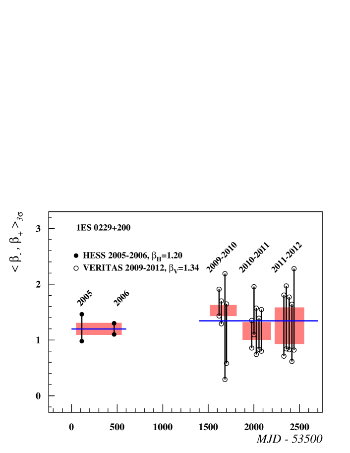
Figure 2: Confidence intervals at a $3\sigma$ level of significance for the source parameter $\beta$ of 1ES 0229+200 are depicted. Lines with full points and red box represent yearly measurements done by the H.E.S.S. instrument [8]. Lines with circles and red boxes refer to the monthly observations during the 2009–2012 VERITAS campaign [7]. Blue lines show the maximum likelihood estimates of the source parameters.

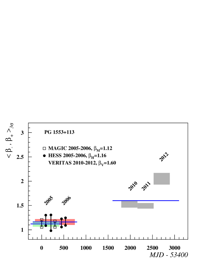
Figure 3: Confidence intervals at a $3\sigma$ level of significance for the source parameter $\beta$ of PG 1553+113 are shown. Green and red boxes are for estimates using the MAGIC and H.E.S.S. data [9, 10]. Grey boxes are for three individual on–off measurements reported by the VERITAS team [11]. Blue lines correspond to the maximum likelihood estimates of the source parameters.

3 Examples

Within the proposed on–off method we examined VHE data for three objects. Specifically, we calculated test statistics $T$ as well as corresponding $p$–values and significances $S$ when testing intensity changes in a series of on–off measurements, see Section 2.1. If possible, we give confidence intervals for the ratio of the numbers of the on–source and background events, as described in Section 2.2. Our results are summarized in Table 1 and in Figs. 1–3.

3.1 1ES 1959+650

The blazar 1ES 1959+650 was observed by the VERITAS setup between April 17, 2012 and June 1, 2012 (MJD 56034 and 56079) [7]. Typically, hundreds of VHE $\gamma$–ray events ($E>315\,{\rm GeV}$) were registered in each of the three reported observations. A steady VHE flux of photons was rejected based on the light curve analysis with a very small $p$–value [7].

Results of our on–off analysis are shown in Table 1 and in Fig. 1. The on–off data taken from Ref. [7] implies that the conjecture of a constant flux is rejected at a significance level of $S\approx 6.37$ ($p$–value $\approx 10^{-10}$). For the three individual observations we also provide in Fig. 1 confidence intervals for the source parameter $\beta$ at a $3\sigma$ level of confidence. None of derived limits corresponds to the overall value of the source parameter ($\hat{\beta}_{0}\approx 4.89$) at a $3\sigma$ level of confidence. We learned that it suffices to judge the on–off data in order that changes of the source intensity were detected from the 1ES 1959+650 object.

3.2 1ES 0229+200

We employed the modified on–off scheme to investigate changes of the VHE $\gamma$–ray intensity associated with the BL Lac object 1ES 0229+200. The data used for this purpose comprise the results of the 2005–2006 observations by the H.E.S.S. instrument [8] as well as the 2009–2012 campaign of the VERITAS collaboration [7]. The numbers of registered on– and off–source events in two yearly H.E.S.S. measurements ($E>580\,{\rm GeV}$) were above two hundred in 2005 and even above one thousand in 2006. The three years campaign ($E>300\,{\rm GeV}$) conducted by the VERITAS experiment provided 14 month–long data sets with the numbers of events ranging from tens to several thousands.

Our on–off results are in agreement with the conclusion of the H.E.S.S. collaboration [8]. When examining these two measurements we found no support for the claim that the source intensity changed between 2005 and 2006, see Table 1 and Fig. 2.

The evidence for variability present in the data sets has been advocated by the VERITAS team using the analysis of light curve [7]. Our on–off results presented in Table 1 allow us to soundly rule out that the source emission registered by the VERITAS setup is consistent with the long–term baseline intensity ($\hat{\beta}_{0}=1.34$) at a high level of significance, $S\approx 4.69$ ($p$–value $\approx 10^{-6}$). The extraordinary nature of the 2009–2010 VERITAS observations is also documented in Fig. 2 where the time sequences of the $\beta$–intervals are depicted. While most of the monthly data are consistent with background, the first monthly period in the 2009–2010 campaign is easily linked with a $3\sigma$ excess of measured counts above the three–years baseline activity.

3.3 PG 1553+113

The observations of BL Lac PG 1553+113 were performed by the MAGIC, H.E.S.S. as well as VERITAS instruments [9, 10, 11]. The light curve measured by the MAGIC telescopes in 2005 and 2006 ($E>200\,{\rm GeV}$) showed no significant variations on a daily time scale [9]. Also, no evidence for the flux variation was detected during the 2 years of observations of the BL Lac PG 1553+113 by the H.E.S.S. setup ($E>200\,{\rm GeV}$) in the 2005–2006 campaigns [10]. The reported data set collected in the years 2010, 2011 and 2012 by the VERITAS instrument [11] contains three yearly measurements of thousands of detected events. These VERITAS observations lead to the conclusion that the averaged flux detected in 2012 was increased by a factor 1.5 and 1.9 with respect to the 2010 and 2011 observations, respectively.

In our on–off analysis presented in Table 1 and in Fig. 3, we did not find any indication of intensity changes in the data collected by the MAGIC and H.E.S.S. telescopes. On the other hand, when the on–off test is performed with the VERITAS data, a clear signature of an extraordinary observation registered in 2012 is returned. This finding exhibits itself in a significance of $S\approx 6.36$ ($p$–value $\approx 10^{-10}$) when the on–off test of the constant source activity is used.

4 Conclusions

We studied changes of a signal in a chosen region when individual measurements of the number of source events are accompanied by events due to background. Based on the properties of the Poisson process, we introduced the asymptotic on–off test for the hypothesis that assumes a constant ratio of the source and background activity in the on–source region. We described the construction of confidence intervals for the source intensity when expressed in terms of background.

The modified significance formulas were applied to the on–off data collected from three VHE $\gamma$–ray emitters. We showed that, independently of the previous analysis, changes of the source activity are reliably quantified using on– and off–source counts. The proposed on–off scheme is not only supported by convincing statistical motivation, but also relatively easy to use, yet sufficiently general. Its independence of the complex estimation of detection conditions makes it suitable for exploring different types of intensity changes in different contexts.

- [1] T.P.Li, Y.Q.Ma, Analysis method for results in gamma-ray astronomy, ApJ 272 (1983) 317.
- [2] G.Cowan, K.Cranmer, E.Gross, O.Vitells, Asymptotic formulae for likelihood–based tests of new physics, EPJ C71 (2011) 1554; and C73 (2011) 2501 [1007.1727v3].
- [3] R.D.Cousins, J.T.Linnemann, J.Tucker, Evaluation of three methods for calculating statistical significance when incorporating a systematic uncertainty into a test of the background-only hypothesis for a Poisson process, NIM A 595 (2008) 480 [physics/0702156v4].
- [4] W.A.Rolke, A.M.López, A.M., J.Conrad, Limits and confidence intervals in the presence of nuisance parameters, NIM A 551 (2005) 493 [physics/0403059v5].
- [5] S.S.Wilks, The large-sample distribution of the likelihood ratio for testing composite hypotheses, Ann.Math.Stat. 9 (1938) 60.
- [6] E.Aliu et al., Investigating broadband variability of the TeV blazar 1ES 1959+650, ApJ 797 (2015) 89 [1412.1031v1].
- [7] S.Aliu et al., A three–year multi–wavelength study of the very–high–energy –ray blazar 1ES 0229+200, ApJ 782 (2014) 13 [1312.6592v1].
- [8] F.Aharonian et al., New constraints on the mid–IR EBL from the HESS discovery of VHE –rays from 1ES 0229+200, A&A 475 (2007) L9 [0709.4584v1].
- [9] J.Albert et al., Detection of very high energy radiation from BL Lacertae object PG 1553+113 with the MAGIC telescope, ApJ 654 (2007) L119.
- [10] F.Aharonian et al., HESS observations and VLT spectroscopy of PG 1553+113, A&A 477 (2008) 481 [0710.5740v2].
- [11] E.Aliu et al., VERITAS observations of the BL Lac object PG 1553+113, ApJ 799 (2015) 7 [1411.1439v1].