Please cite as: Garbuno-Inigo, Alfredo, Francisco Alejandro DiazDelaO, and Konstantin M. Zuev. Transitional annealed adaptive slice sampling for Gaussian process hyper-parameter estimation.International Journal for Uncertainty Quantification, 6.4 (2016).
Transitional annealed adaptive slice sampling for Gaussian process hyper-parameter estimation

Abstract

Surrogate models have become ubiquitous in science and engineering for their capability of emulating expensive computer codes, necessary to model and investigate complex phenomena. Bayesian emulators based on Gaussian processes adequately quantify the uncertainty that results from the cost of the original simulator, and thus the inability to evaluate it on the whole input space. However, it is common in the literature that only a partial Bayesian analysis is carried out, whereby the underlying hyper-parameters are estimated via gradient-free optimisation or genetic algorithms, to name a few methods. On the other hand, maximum a posteriori (MAP) estimation could discard important regions of the hyper-parameter space. In this paper, we carry out a more complete Bayesian inference, that combines Slice Sampling with some recently developed Sequential Monte Carlo samplers. The resulting algorithm improves the mixing in the sampling through delayed-rejection, the inclusion of an annealing scheme akin to Asymptotically Independent Markov Sampling and parallelisation via Transitional Markov Chain Monte Carlo. Examples related to the estimation of Gaussian process hyper-parameters are presented. For the purpose of reproducibility, further development, and use in other applications, the code to generate the examples in this paper is freely available for download at http://github.com/agarbuno/ta2s2_codes.

1 Introduction

The use of computationally expensive computer codes is widespread in science and engineering in order to simulate and investigate complex phenomena. Such codes, also referred to as simulators, often require intensive use of computational resources that allows their use in contexts such as optimisation, uncertainty analysis and sensitivity analysis (Forrester et al., 2008, Kennedy and O’Hagan, 2001a). For this reason, surrogate models are needed to efficiently approximate the output of demanding simulators and enable efficient exploration and exploitation of the input space. In this context, Gaussian processes are a common choice to build statistical surrogates -also known as emulators- which account for the uncertainty that stems from the inability to evaluate the original model in the whole input space. Gaussian processes are able to fit complex input/output mappings through a non-parametric hierarchical structure. Common applications of Gaussian processes are found in Machine Learning (Rasmussen and Williams, 2006), Spatial Statistics (Cressie, 1993) (with the name of Kriging), likelihood-free Bayesian Inference (Wilkinson, 2014), Genetics (Kalaitzis and Lawrence, 2011) and Engineering (DiazDelaO and Adhikari, 2011), amongst many other areas.

Building an emulator requires the simulator to be run a repeated number of times, but due to its computational complexity only a limited amount of evaluations is available. This cost often translates in an inadequate explanation of the uncertainty of the model parameters by uni-modal probability distributions. This phenomenon is often encountered in the form of low signal-to-noise ratio which translates into multi-modal distributions of the parameters (Warnes and Ripley, 1987). Although it is not pathological in terms of the Gaussian process predictive performance, this might lead to solutions with no significant meaning for the parameters of the surrogate. The Bayesian treatment of the inference problem often alleviates this concern by means of the prior, however multi-modality cannot be fully discarded (Andrianakis and Challenor, 2012). In this setting, where the information available to train a Gaussian process is limited, one is able to acknowledge all uncertainties related to the modelling assumptions by resorting to Model Uncertainty Analysis (Draper, 1995). More specifically, hierarchical modelling should be considered in the model formulation. By doing so, the analyst is capable of accounting for structural uncertainty, which can be considered either as a continuous or discrete construct (see Draper, 1995, §4). In Gaussian processes models, continuous structural uncertainty can be incorporated through the Bayesian paradigm. In this work, the approach for dealing with different models which are originated from multi-modal distributions of the model parameters is to employ samplers specifically built for such scenarios.

The implementation of a Gaussian process emulator requires a training phase. This involves the estimation of the parameters of the Gaussian process, referred to as hyper-parameters. The selection of the hyper-parameters is usually done by Maximum Likelihood estimates (MLE) (Forrester et al., 2008), Maximum a Posteriori estimates (MAP) (Oakley, 1999, Rasmussen and Williams, 2006), or by sampling from the posterior distribution (Williams and Rasmussen, 1996) in a fully Bayesian manner. It is frequently the case that estimating the hyper-parameters depends on maximising a complex, multi-modal function. In this scenario, traditional optimisation routines (Nocedal and Wright, 2004) are not able to guarantee global optima when looking for the MLE or MAP, and a Bayesian treatment becomes a suitable option to account for all the uncertainties in the modelling. In the literature however, it is common that either the MLE or MAP alternatives are preferred (Kennedy and O’Hagan, 2001a, Gibbs, 1998) due to the numerical burden of maximising the likelihood function or because it is assumed that Bayesian integration (for example, through Markov chain Monte Carlo methods) is prohibitive. Although these are strong arguments in favour of point estimates, in high-dimensional applications it is difficult to assess if the number of runs of the simulator is sufficient to produce robust hyper-parameters. This is usually measured with prediction-oriented metrics such as the root-mean-square error (RMSE) (Kennedy and O’Hagan, 2001b). The use of this metric ignores the uncertainty and risk assessment of choosing a single candidate for the hyper-parameters through an inference process with limited data. In order to account for such uncertainty, numerical integration should be performed. However, methods such as quadrature approximation become quickly infeasible as the number of dimensions increases (Kennedy and O’Hagan, 2001a). Therefore, a suitable approach is to perform Monte Carlo integration (MacKay, 1998). This allows to approximate any integral by means of a weighted sum, given a sample from the correct distribution.

The Gaussian process model specification yields no direct simulation of its hyper-parameters by means of standard distributions (Gaussian, uniform or exponential, to name a few). In order to be able to approximate the related integrals, Markov chain Monte Carlo (MCMC) provides the proper statistical tool to generate a desired sample. Nonetheless, the canonical sampling schemes, such as Metropolis-Hastings or Gibbs sampling, might no be appropriate for multi-modal distributions (Neal, 2001, Hankin, 2005). This limitation is originated by the tuning of the proposal distribution, the function used to generate samples. If it is not correctly specified, the sampling space might not be properly explored. The efficiency of the sampler should balance the ability to move freely through the sampling space as well as to generate candidates according to the regions where the probability mass is concentrated. One of the most recognised concerns in simulation is to avoid Random Walk behaviour, since it delays the stationarity state achieved by the chain and limits its exploration capabilities (Neal, 1993). An optimal tuning of the proposal distribution in high-dimensional spaces with intricate correlation among sets of variables can turn into a demanding task yielding MCMC samplers expensive (Ching and Chen, 2007). One alternative in Gaussian processes, amongst other probabilistic applications, is to resort to the Hybrid Monte Carlo (HMC) sampler, as it can avoid Random Walk behaviour at the expense of additional computations needed for the gradient of the posterior (Neal, 1998, Williams and Rasmussen, 1996). However, there is no guarantee that multi-modal distributions can be sampled thoroughly by HMC (Neal, 2011) and in Gaussian process models the gradients are not available in $\mathcal{O}(n)$ operations.

This paper proposes a sampling scheme for multi-modal distributions based on two principles. Firstly, the concept of crumb introduced by Neal (2003) for a multivariate adaptive slice sampler. Secondly, the ideas by Zuev and Beck (2013) on how to simulate local approximations to the solution based on a sequence of nested subsets as in Stochastic Subset Optimisation (Taflanidis and Beck, 2008a, b). The use of delayed rejection in the Asymptotically independent Markov sampler (Garbuno-Inigo et al., 2015) has proven to enhance the mixing capabilities of the algorithm in highly correlated probability models. To our knowledge, coupling the adaptive slice sampling algorithm with a sequential sampler has not been explored previously. This presents an opportunity to develop efficient sampling algorithms for multi-modal distributions. The main advantage of the proposed scheme is that it requires little tuning of parameters as it automatically learns the sequence of temperatures for an annealing schedule, as opposed to being tuned by trial and error (Birge and Polson, 2012). The approximation set simulated in the previous level can be exploited further as it provides the crumbs needed for the sampling in the next annealing level, leading the simulation to appropriate regions of the sampling space. Additionally, embedding the sampler with the Transitional Markov chain Monte Carlo method (Ching and Chen, 2007) results in an algorithm that can be run in a cluster of cores, if available. By using the proposed Transitional Annealed Adaptive Slice Sampling (TA²S²) algorithm to sample the hyper-parameters of a Gaussian process, the resulting emulator is built taking into account both a probabilistic and computationally efficient perspective. The probabilistic strategy to treat the problem in a Bayesian manner accounts for the uncertainty that stems from the unknown parameters. This adds a layer of structural uncertainty to the model. Additionally, model uncertainty is accounted for by adding numerical stabilisation measures in the Gaussian process model as in Ranjan et al. (2011), Andrianakis and Challenor (2012) in a fully Bayesian framework.

The paper is organised as follows. In Section 2, a brief introduction to the Bayesian treatment of Gaussian processes, as well as related numerical stabilisation procedures, are presented. Section 3 briefly reviews the concepts of Slice Sampling and Adaptive Slice Sampling. Section 4 presents the proposed algorithm with the concepts discussed in the previous sections, as well as the extensions needed for a parallel implementation. In Section 5, some illustrative examples are used to discuss the efficiency and robustness of the proposed algorithm. Concluding remarks are presented in Section 6.

2 The Gaussian process model

Let the real-valued function $\eta:\mathbb{R}^{p}\rightarrow\mathbb{R}$ represent the underlying input/output mapping of a computer model. Let $X=\{\mathbf{x}_{1},\ldots,\mathbf{x}_{n}\}$ be the set of design points, that is, the set of selected points in the input space, where $\mathbf{x}_{i}\in\mathbb{R}^{p}$ denotes a given input configuration. Let $\mathbf{y}=\{y_{1},\ldots,y_{n}\}$ be the corresponding set of outputs $y_{i}=\eta(\mathbf{x}_{i})$, such that each pair $(\mathbf{x}_{i},y_{i})$ denotes a training run. The emulator is assumed to be an interpolator for the training runs, i.e. $y_{i}=\tilde{\eta}(\mathbf{x}_{i})$ for all $i=1,\ldots,n$, where the tilde denotes approximation. This omits any random error in the output of the computer code in the observed simulations, for which the simulator is said to be deterministic. If a fully parametrised Gaussian process prior is assumed for the outputs of the simulator, then the set of design points has a joint Gaussian distribution. The general assumption is that the simulator satisfies the statistical model for the output with the following structure

$$\eta(\mathbf{x})=h(\mathbf{x})^{\top}\boldsymbol{\beta}+Z(\mathbf{x}|\sigma^{2},\boldsymbol{\phi}),$$ (2.1)

where $h(\cdot)$ is a vector of known basis (location) functions of the input, $\boldsymbol{\beta}$ is a vector of regression coefficients, and $Z(\cdot|\sigma^{2},\boldsymbol{\phi})$ is a Gaussian process with zero mean and covariance function

$$\text{cov}(\mathbf{x},\mathbf{x}^{\prime}|\sigma^{2},\boldsymbol{\phi})=\sigma^{2}\,k(\mathbf{x},\mathbf{x}^{\prime}|\boldsymbol{\phi}),$$ (2.2)

where $\sigma^{2}$ is the signal noise and $\boldsymbol{\phi}\in\mathbb{R}^{p}_{+}$ denotes the length-scale parameters of the correlation function $k(\cdot,\cdot)$. The hyper-parameters of the Gaussian process are therefore $\boldsymbol{\theta}=(\boldsymbol{\beta},\sigma^{2},\boldsymbol{\phi})$. For practical simplicity it is commonly assumed that $h(\mathbf{x})=0$. This allows to perform predictions and quantify the underlying uncertainty by relying completely in the covariance function to capture the dependencies among training runs. Thus $\boldsymbol{\beta}$ is dropped out of the discussion in the remainder. Note that for a pair of design points $(\mathbf{x},\mathbf{x}^{\prime})$, the function $k(\cdot,\cdot|\boldsymbol{\phi})$ measures the correlation between $\eta(\mathbf{x})$ and $\eta(\mathbf{x}^{\prime})$ based on their respective input configurations. The correlation function is capable of measuring how close different input configurations are, such that related inputs produce related outputs in the simulator. The base of such measure is related to the Euclidean distance in such a way that it weights differently each input variable. In this work, the squared-exponential correlation function has been chosen due to its tractability, namely

$$k(\mathbf{x},\mathbf{x}^{\prime}|\boldsymbol{\phi})=\exp\left\{-\frac{1}{2}\displaystyle\sum_{i=1}^{p}\frac{(x_{i}-x^{\prime}_{i})^{2}}{\phi_{i}}\right\}.$$ (2.3)

It is important to note that other authors (Neal, 1998, Rasmussen and Williams, 2006, Murray et al., 2009) prefer the $\phi^{2}_{i}$ parameterisation in the denominator. In our case, it is more natural to use a linear term, given that the length-scale parameters are restricted to lie in the positive orthant. The linear terms can be interpreted as weights in the norm used to measure closeness and sensitivity to changes in each dimension.

As a consequence of the Gaussian process prior, the joint probabilistic model for the vector of outputs $\mathbf{y}$, given the hyper-parameters $\sigma^{2}$, $\boldsymbol{\phi}$ and the design points $X$, can be written as

$${\bf y}|X,\sigma^{2},\boldsymbol{\phi}\sim\mathcal{N}(0,\sigma^{2}\,K),$$ (2.4)

where $K$ is the correlation matrix with elements $K_{ij}=k(\mathbf{x}_{i},\mathbf{x}_{j}|\boldsymbol{\phi})$ for all $i,j=1,\ldots,n$.

2.1 Hyper-parameter marginalisation

The hyper-parameters of the Gaussian process emulator are commonly unknown before the training phase, which adds uncertainty to the surrogate. A common practice in the literature is to fix them to their Maximum Likelihood value. Though it has been widely accepted, this approach does not entirely treat the emulator as a probabilistic model and uncertainty quantification through it might become limited. On the other hand, if one acknowledges the parameters as random variables, robust estimators can be built through numerical integration by marginalising them via samples generated from their posterior distribution. Predictions for $y^{*}$, given a non-observed configuration $\mathbf{x}^{*}$, can be performed using all the evidence provided by the available data $\mathcal{D}=({\bf y},X)$, exploiting the posterior distribution of the hyper-parameters, namely

$$p(y^{*}|\mathbf{x}^{*},\mathcal{D})=\int_{\Theta}p(y^{*}|\mathbf{x}^{*},\mathcal{D},\boldsymbol{\theta})\,p(\boldsymbol{\theta}|\mathcal{D})\,d\boldsymbol{\theta},$$ (2.5)

where $\boldsymbol{\theta}=(\sigma^{2},\boldsymbol{\phi})$ denotes the vector of hyper-parameters. Note that the model used for predictions $y^{*}$, given the data and $\boldsymbol{\theta}$, is a Gaussian random variable, which makes the model closed under the Gaussian family (see Oakley, 1999).

By means of a sample from the posterior distribution, the mean and covariance functions of the predictive posterior can be written through a mixture of Gaussians (Garbuno-Inigo et al., 2015) as

$$\mu(\mathbf{x}^{*}) =\sum_{i=1}^{N}w_{i}\,\,\mu_{i}(\mathbf{x}^{*}),$$ (2.6)

$$\text{cov}(\mathbf{x}^{*},\mathbf{x}^{\prime}) =\sum_{i=1}^{N}w_{i}\,\,\left[(\mu_{i}(\mathbf{x}^{*})-\mu(\mathbf{x}^{*}))(\mu_{i}(\mathbf{x}^{\prime})-\mu(\mathbf{x}^{\prime}))+\text{cov}(\mathbf{x}^{*},\mathbf{x}^{\prime}|\boldsymbol{\theta}_{i})\right],$$ (2.7)

where $\mu_{i}(\mathbf{x}^{*})$ is the expected value of the probability model of $y^{*}$ conditional on the hyper-parameters $\boldsymbol{\theta}_{i}$, the training runs $\mathcal{D}$ and the input configuration $\mathbf{x}^{*}$. From equation (2.7) it follows that the variance (also known as the prediction error) of an untested configuration $\mathbf{x}^{*}$ is

$$s^{2}(\mathbf{x^{*}}) =\sum_{i=1}^{N}w_{i}\,\,((\mu_{i}(\mathbf{x^{*}})-\mu(\mathbf{x^{*}}))^{2}+s_{i}^{2}(\mathbf{x^{*}})).$$ (2.8)

This results in a more robust estimation of the prediction error, since it balances the predicted error in one sample with how far the prediction of such sample is from the overall estimation of the mixture.

2.2 Prior distributions

The predictive posterior distribution in equation (2.5) requires the specification of a prior distribution $p(\sigma^{2},\boldsymbol{\phi})$. Weak prior distributions have been used for $\boldsymbol{\phi}$ and $\sigma^{2}$ (Oakley, 1999), namely

$$p(\sigma^{2},\boldsymbol{\phi})\propto\frac{p(\boldsymbol{\phi})}{\sigma^{2}},$$ (2.9)

where $\sigma^{2}$ is assumed to have a non-informative distribution. For the length-scale hyper-parameters $\boldsymbol{\phi}$, the reference prior (Berger and Bernardo, 1992, Berger et al., 2009) allows for an objective framework in which the uncertainty of $\boldsymbol{\phi}$ can be accounted for. It requires no previous knowledge, such that the training runs are the only source of information for the inference process. Additionally, the reference prior is capable of ruling out subspaces of the sample space of the hyper-parameters (Andrianakis and Challenor, 2011), thus reducing regions of possible candidates in the mixture model expressed in equations (2.6), (2.7) and (2.8). This allows for prior distributions without concerns about expert knowledge of feasible regions for the hyper-parameters. Unless otherwise stated, the reference prior for Gaussian processes developed by Paulo (2005) is used in this work. Note however that there are no known analytical expressions for the derivatives of this prior, which limits its application to samplers that require first-order information like HMC. Additionally, it is important to note that there are other possibilities available for the prior distribution of $\boldsymbol{\phi}$. Examples of these are the log-normal or log-Laplacian distributions, which can be interpreted as a regularisation in the norm of the parameters. Other alternatives suggest a decaying prior (Andrianakis and Challenor, 2011) or a weakly informative distribution such as a gamma with appropriate parameters. If needed, elicited priors from experts can also be used (Oakley, 2002).

2.3 Marginalising the nuisance hyper-parameters

The hyper-parameters $\boldsymbol{\phi}$ and $\sigma^{2}$ may be potentially different in terms of scales and dynamics, as explained previously in Garbuno-Inigo et al. (2015). Gibbs sampling might help with this limitation, although it is well-known that such sampling scheme can be inefficient when used for multi-modal distributions in high-dimensional spaces. The Metropolis-Hastings sampler exhibits the same problem. For this reason, this work focuses on $\boldsymbol{\phi}$ to perform the inference based in the correlation function. To achieve this, $\sigma^{2}$ is considered as a nuisance parameter and is integrated out from the posterior. This way, all inference is driven by the length-scale hyper-parameters of the correlation function. Note that other authors follow different approaches in the inference problem of Gaussian processes as emulators. For example, Vernon et al. (2010) focus on the global trend function $h(\cdot)^{\top}\boldsymbol{\beta}$ since it allows to incorporate expert knowledge on the computer model being emulated. That is, a fully parametrised Gaussian process is considered. The probability model of the training runs and the prior distribution of the hyper-parameters (equations (2.4) and (2.9)) allow to identify an inverse-gamma model for $\sigma^{2}$, which after integration, can be shown to yield the integrated posterior distribution

$$p(\boldsymbol{\phi}|\mathcal{D})\propto p(\boldsymbol{\phi})\,(\hat{\sigma}^{2})^{-\frac{n-p}{2}}\,|K|^{-\frac{1}{2}},$$ (2.10)

where

$$\hat{\sigma}^{2} =\frac{\mathbf{y}^{\top}\,K^{-1}\,\mathbf{y}}{n-1}$$ (2.11)

is an estimator of the signal noise $\sigma^{2}$ (see Oakley, 1999, for further details). Finally, the predictive distribution conditioned on the remaining set of hyper-parameters, $\boldsymbol{\phi}$, follows a t-student distribution with mean and correlation functions

$$\mu(\mathbf{x}^{*}|\boldsymbol{\phi})= \,\,t(\mathbf{x}^{*})^{\top}K^{-1}\mathbf{y},$$ (2.12)

$$\text{corr}(\mathbf{x}^{*},\mathbf{w}^{*}|\boldsymbol{\phi})= \,\,k(\mathbf{x}^{*},\mathbf{w}^{*}|\boldsymbol{\phi})-t(\mathbf{x}^{*})^{\top}K^{-1}\,t(\mathbf{w}^{*}),$$ (2.13)

where $\mathbf{x}^{*}$, $\mathbf{w}^{*}$ denote a pair of untested configurations and $t(\mathbf{x}^{*})$ denotes the vector obtained by computing the covariance of a new input configuration with every design point available for training $t(\mathbf{x})=(k(\mathbf{x},\mathbf{x}_{1}|\boldsymbol{\phi}),\ldots,k(\mathbf{x},\mathbf{x}_{n}|\boldsymbol{\phi}))^{\top}$. Note that both the mean and the correlation of unseen input configurations depend solely on the correlation function hyper-parameters $\boldsymbol{\phi}$. MacKay (1996) has previously discussed the treatment of nuisance parameters and integrated posteriors. In the context of Gaussian process emulators, this discussion allows to overcome the limitations of samplers when faced to different dynamics posed by each subset of hyper-parameters.

In light of the above, this paper focuses on the correlation function $k(\cdot,\cdot)$ in equation (2.2), since the structural dependencies of the training runs to allow prediction in the outputs of the simulator is recovered by it.

2.4 Numerical stability

Numerical stability is usually difficult to guarantee when implementing Gaussian processes. As explored previously by Andrianakis and Challenor (2012) and Ranjan et al. (2011), a term can be added in the covariance matrix $K$ in order to preserve diagonal dominancy, that is, to add a nugget hyper-parameter $\boldsymbol{\phi}_{\delta}$ such that

$$K_{\delta}=K+\boldsymbol{\phi}_{\delta}\,I,$$ (2.14)

is positive definite. This results in the stochastic simulator

$$y_{i}=\eta(\mathbf{x}_{i})+\sigma^{2}\,\boldsymbol{\phi}_{\delta},$$ (2.15)

where the term $\sigma^{2}\,\boldsymbol{\phi}_{\delta}$ is used to account for the variability of the simulator that cannot be explained by the correlation function. The inclusion of the nugget modifies the posterior distribution, and possibly adds new modes. In such scenario, the use of multi-modal oriented samplers is crucial for performing the Monte Carlo approximation of equation (2.5). In case that the resulting model is assessed as not appropriate, a regularisation term (an elicited prior) can be added to penalise regions of local modes (Andrianakis and Challenor, 2012).

As previously discussed by Ranjan et al. (2011), a uniform prior distribution $U(10^{-12},1)$ is adopted for the nugget hyper-parameter $\phi_{\delta}$. The lower bound guarantees stability in computations associated with the covariance matrix. The upper bound forces the numerical noise of the simulator to be smaller than the signal noise of the emulator itself. By considering the modified correlation matrix in equation (2.14), the previous assumptions regarding the original noise parameter $\sigma^{2}$ remain unchanged, as one can still marginalise it as a nuisance parameter with the non-informative prior used (De Oliveira, 2007).

3 Slice sampling

The slice sampling algorithm (Neal, 2003) is a method to simulate a Markov chain of a random variable $\boldsymbol{\theta}\in\Theta$. This is done by introducing an auxiliary random variable $u\in\mathcal{U}\subseteq\mathbb{R}$ and sampling from the joint distribution on the extended space $\Theta\times\mathcal{U}$. The marginal of $\boldsymbol{\theta}$ is recovered by disregarding the values of $u$ in the Markov chain, a consequence of defining an appropriate conditional distribution for $u$, given $\boldsymbol{\theta}$. The samples are generated by an iterative Gibbs sampling schedule to recover pairs $\{(\boldsymbol{\theta}_{i},u_{i})\}_{i=1}^{N}$, which follow the joint density probability distribution

$$\pi(\boldsymbol{\theta},u)\propto I_{\{u<\pi(\boldsymbol{\theta})\}}(\boldsymbol{\theta},u),$$ (3.1)

where $I_{E}(\cdot)$ is the indicator function for the set $E\subset\Theta\times\mathcal{U}$, and $\pi(\boldsymbol{\theta})$ is the target distribution of $\boldsymbol{\theta}$. Slice Sampling first generates $u$ from the conditional distribution of $u\,|\,\boldsymbol{\theta}$ specified as a uniform on the interval $(0,\pi(\boldsymbol{\theta}))$. It then samples $\boldsymbol{\theta}$, conditioned in $u$ from a uniform distribution in the slice defined by the set

$$S_{u}=\{\boldsymbol{\theta}:u<\pi(\boldsymbol{\theta})\}.$$ (3.2)

Since the marginal satisfies $\int_{0}^{\pi(\boldsymbol{\theta})}\pi(\boldsymbol{\theta},u)\,du=\pi(\boldsymbol{\theta})$, samples from the target distribution can be recovered by disregarding the auxiliary component of the joint samples. If the target distribution is a non-normalised probability density $f(\boldsymbol{\theta})$ then the joint distribution can be written as

$$\pi(\boldsymbol{\theta},u)=\frac{1}{Z}\,I_{\{u<f(\boldsymbol{\theta})\}}(\boldsymbol{\theta},u),$$ (3.3)

where $Z=\int_{\Theta}f(\boldsymbol{\theta})\,d\boldsymbol{\theta}$ and the previous considerations for the marginal of $\boldsymbol{\theta}$ follow. In the context of Gaussian processes it should be noted that floating-point underflows are common due to ill-conditioning of the matrix $K$ in equation (2.10). Thus, in order to compute stable evaluations of the target distribution in Slice Sampling, it is preferable to evaluate the negative logarithm of the target density. In such case, equation (3.2) can be computed as stated in the following proposition.

Proposition 1.

Given the state of the Markov chain $\boldsymbol{\theta}_{0}$, the uniform distribution for the next candidate has support in the slice given by

$$S_{\boldsymbol{\theta}_{0}}=\{\boldsymbol{\theta}:z>\mathcal{H}(\boldsymbol{\theta})\},$$ (3.4)

where $\mathcal{H}(\cdot)$ denotes the negative logarithm of the target density and $z=\mathcal{H}(\boldsymbol{\theta}_{0})+e$, with $e$ distributed as an exponential random variable with mean equal to 1.

Proof.

The result follows from the fact that for a given state $\boldsymbol{\theta}_{0}$ of the Markov chain, the auxiliary uniform random variable defining the slice can be written as the product $u\,f(\boldsymbol{\theta}_{0})$ with $u$ uniformly distributed in the interval $(0,1)$. Thus, the slice is defined as

$$S_{\boldsymbol{\theta}_{0}} =\{\boldsymbol{\theta}:u\,f(\boldsymbol{\theta}_{0})<f(\boldsymbol{\theta})\}$$

$$=\{\boldsymbol{\theta}:-\log(f(\boldsymbol{\theta}_{0}))-\log(u)>-\log(f(\boldsymbol{\theta}))\}$$

$$=\{\boldsymbol{\theta}:\mathcal{H}(\boldsymbol{\theta}_{0})+e>\mathcal{H}(\boldsymbol{\theta})\},$$ (3.5)

where it is easy to prove that $e=-\log(u)$ is distributed as an exponential random variable with mean 1 and $\mathcal{H}(\cdot)$ denotes the negative logarithm of the target density. ∎

The main concern when implementing Slice Sampling is the ability to sample uniformly from the slice. In one-dimensional applications, the slice can be defined by several methods. The canonical example is a stepping-out and shrinkage procedure which aims to extend an initial interval until the edges are outside the slice and then shrinking it as samples generated from the interval are rejected (see Neal, 2003, for further details).

3.1 Adaptive slice sampling

For multivariate distributions, the concept of the slice extends naturally. However, methods based on intervals (e.g. the stepping-out and shrinking procedure) slow dramatically as the dimension of the problem increases. This is due to the generalisation of intervals as hyper-rectangles in $\mathbb{R}^{p}$ and the need to compute the target function for each vertex a repeated number of times along the expansion and shrinkage of the boundaries. For Gaussian process emulators, the task of evaluating the target density becomes expensive, a consequence of the non-parametric nature of the model and the computational cost of evaluating equation (2.5). If multiple evaluations are needed for the construction of the Markov chain either because of a high rejection rate, difficult characterisation of the slice or if longer chains are required, simulation by MCMC with slice sampling becomes computationally expensive and inefficient. Therefore, other alternatives are preferable.

This work employs a framework proposed by Neal (2003) for adaptive slice sampling in multivariate applications. The key idea is the use of the information provided by the rejected samples in order to lead the future generation of a candidate inside the slice. In this framework, the evidence gathered by the rejected candidates is referred to as crumbs, as they will be “followed” towards the slice. For a more detailed discussion see (Neal, 2003).

4 Transitional annealed adaptive slice sampling

As previously stated, in order to marginalise the posterior predictive distribution in equation (2.5), Monte Carlo integration is usually performed when aiming at a fully Bayesian treatment of Gaussian process surrogates. This is usually done by Hybrid Monte Carlo (Neal, 1998, Williams and Rasmussen, 1996) which is capable of suppressing the Random Walk behaviour of traditional MCMC methods. Nonetheless, the tuning of this kind of algorithm is problem-dependent and expert knowledge is crucial for an optimal sampling schedule. The development of Elliptical Slice Sampling (Murray et al., 2009) provides a framework for the simulation of the hyper-parameters of a Gaussian process with little tuning required from the analyst (Murray and Adams, 2010). However, this is only applicable when the posterior predictive distribution for the hyper-parameters is of the form

$$p(\boldsymbol{\theta}|\mathcal{D})\propto\mathcal{N}(l(\boldsymbol{\theta})|\boldsymbol{\mu},\Sigma)\,p(\boldsymbol{\theta}),$$ (4.1)

where $p(\boldsymbol{\theta})$ denotes the prior distribution, $\mathcal{N}(\cdot|\cdot,\cdot)$ is a Gaussian distribution and $l(\cdot)$ is a latent variable that depends on the hyper-parameters. As it can be seen from the integrated posterior in equation (2.10), this form is not valid in the formulation followed. The difference stems from $\sigma$ being considered a nuisance parameter and the prior considered for the length-scales of the Gaussian process.

In this setting, we propose Transitional Annealed Adaptive Slice Sampling (TA²S²), which can also be used in other applications of Bayesian inference and Stochastic optimisation. Based on Asymptotically Independent Markov Sampling (Beck and Zuev, 2013) we formulate the sampling problem to be solved as reminiscent of simulated annealing. The objective is to sample from intermediate posterior distributions $p_{k}(\boldsymbol{\phi}|\mathcal{D})$ that eventually converge to the true posterior. This is done by tempering the posterior distribution by means of a monotonically decreasing sequence of temperatures $\tau_{k}$ converging to 1. Let $\{p_{k}(\boldsymbol{\phi}|\mathcal{D})\}_{k=1}^{\infty}$ be the sequence of density distributions in the annealing schedule such that

$$p_{k}(\boldsymbol{\phi}|\mathcal{D}) \propto p(\boldsymbol{\phi}|\mathcal{D})^{1/\tau_{k}}=\exp\left\{-\mathcal{H}(\boldsymbol{\phi}|\mathcal{D})/\tau_{k}\right\},$$ (4.2)

where $\mathcal{H}(\boldsymbol{\phi}|\mathcal{D})$ denotes the negative integrated log-posterior distribution of the length-scale hyper-parameters, given the set of training runs $\mathcal{D}$.

The algorithm provides a sequence of nested subsets $\Phi_{k+1}\subseteq\Phi_{k}$ converging to the set of posterior samples $\Phi^{*}$. The temperature is learned through an automatic mechanism to determine the sequence of distributions.

By construction, the sample in the first level of annealing is distributed uniformly on a practical support of the sampling space (see Katafygiotis and Zuev, 2007, for more a detailed discussion). For the limiting case, the samples are uniformly distributed in the support of the posterior density. Both these observations can be summarised by

$$\lim_{\tau\rightarrow\infty}p_{\tau}(\boldsymbol{\phi}|\mathcal{D}) =U_{\Phi}(\boldsymbol{\phi}),$$ (4.3)

$$\lim_{\tau\rightarrow 1}p_{\tau}(\boldsymbol{\phi}|\mathcal{D}) =U_{\Phi^{*}}(\boldsymbol{\phi}),$$ (4.4)

where $U_{A}(\boldsymbol{\phi})$ denotes a uniform distribution over the set $A$ for every $\boldsymbol{\phi}\in A$.

4.1 Annealing at level k

This subsection focuses on the sampling carried out by TA²S² at the $k$-th level of the annealing sequence. It is therefore assumed that a sample from level $k-1$, which is distributed according to $p_{k-1}(\boldsymbol{\phi}|\mathcal{D})$, has already been generated. Let $\boldsymbol{\phi}_{1}^{(k-1)},\ldots,\boldsymbol{\phi}_{N}^{(k-1)}$ denote such sample and let $N$ be the sample size in each annealing level. Following the ideas discussed in Section 3.1 for Adaptive Slice Sampling, the crumb formulation will be exploited. The samples from the previous level play the role as the crumbs to be followed to generate candidates from each slice. Thus, retaining information from the posterior landscape and limiting the amount of evaluations of the integrated posterior, which can be expensive for a reasonable number of training runs. Firstly, note that Proposition 1 implies the following

Corollary 1.

The slice defined in the $k$-th annealing level, given the current state of the Markov chain $\boldsymbol{\phi}_{0}$, is given by

$$S_{\boldsymbol{\phi}_{0}}^{k}=\{\boldsymbol{\phi}:z_{k}>\mathcal{H}(\boldsymbol{\phi}|\mathcal{D})\},$$ (4.5)

where $z_{k}=\mathcal{H}(\boldsymbol{\phi}_{0}|\mathcal{D})+e_{k}$, with $e_{k}$ an exponential random variable with mean $\tau_{k}$.

As in other Sequential Monte Carlo algorithms (Del Moral et al., 2006, Fearnhead and Taylor, 2013), let us define the importance weights of the samples $\boldsymbol{\phi}_{1}^{(k-1)},\ldots,\boldsymbol{\phi}_{N}^{(k-1)}$ as

$$\omega^{(k-1)}_{j} =\frac{p_{k}\left(\boldsymbol{\phi}^{(k-1)}_{j}\right)}{p_{k-1}\left(\boldsymbol{\phi}^{(k-1)}_{j}\right)}\propto\exp\left\{-\mathcal{H}\left(\boldsymbol{\phi}^{(k-1)}_{j}|\mathcal{D}\right)\left(\frac{1}{\tau_{k}}-\frac{1}{\tau_{k-1}}\right)\right\},$$ (4.6)

$$\overline{\omega}^{(k-1)}_{j} =\frac{\omega^{(k-1)}_{j}}{\sum_{j=1}^{N}\omega^{(k-1)}_{j}},$$ (4.7)

where $\omega^{(k-1)}_{j}$ denotes the importance weights and $\overline{\omega}^{(k-1)}_{j}$ the normalised importance weights. The weights allow to measure the importance of each sample as being drawn for the next annealing level.

The proposal for a new state of the Markov chain, given the current one $\boldsymbol{\phi}_{0}$, is generated as follows. A slice is obtained as in equation (4.5) by generating an exponential random variable with mean $\tau_{k}$, thus defining the slice $S_{\boldsymbol{\phi}_{0}}^{k}$ for the current state. A first crumb is randomly selected from the set of past approximations that lie inside the slice. This means selecting a uniformly distributed index $j$ from the set

$$\mathcal{J}=\left\{j\in\{1,\ldots,N\}\,:\,\boldsymbol{\phi}_{j}^{(k-1)}\in S_{\boldsymbol{\phi}_{0}}^{k}\right\}.$$ (4.8)

The points $\boldsymbol{\phi}_{1}^{(k-1)},\ldots,\boldsymbol{\phi}_{N}^{(k-1)}$ are uniformly distributed in the approximation set $\Phi_{k-1}$ and will be used as markers for the annealing level $k$. If the above index set is empty, there is evidence of the annealing temperature being decreased too rapidly. A fail-safe can be used by generating a crumb from a wide Gaussian distribution centred at the current state of the Markov chain. Additionally, as it is done in other Sequential Monte Carlo methods (Del Moral et al., 2012), a renewal component can be added. The renewal is performed as the crumbs are selected from the markers, due to the fact that relying on the sample from the previous level can lead to bias in the simulations. To this end, if the index set $\mathcal{J}$ is empty or, with probability $p_{\text{renew}}$, the crumb $\boldsymbol{\varsigma}_{1}$ will be distributed as

$$\boldsymbol{\varsigma}_{1}\sim\mathcal{N}(\boldsymbol{\phi}_{0},c_{0}^{2}\,\Sigma_{k}),$$ (4.9)

where $c_{0}$ is a spread parameter associated with the annealing sequence, and $\Sigma_{k}$ denotes a covariance matrix at level $k$. Typical choices for the covariance matrix are the identity matrix $I_{p\times p}$ or a diagonal matrix $\text{diag}\{d_{1},\ldots,d_{p}\}$ which defines a different scale for each variable. In order to use a better proposal in terms of scales and correlations observed along the annealing sequence, we define $\Sigma_{k}$ as the weighted covariance matrix from the weighted samples $\{(\overline{\omega}^{(k-1)}_{j},\boldsymbol{\phi}_{j}^{(k-1)})\}_{j=1}^{N}$. As discussed by (Gelman et al., 1996), the spread parameter is set as $c_{0}=2.38/\sqrt{p}$, since it allows for efficient transitions in Gaussian steps.

Once the first crumb is drawn, a first candidate $\boldsymbol{\xi}_{1}$ is generated from the appropriate Gaussian distribution

$$\boldsymbol{\xi}_{1}\sim\mathcal{N}(\boldsymbol{\varsigma}_{1},c_{0}^{2}\,\Sigma_{k}),$$ (4.10)

where $c_{0}$ is a spread parameter for the proposals and $\Sigma_{k}$ defined as above. In general, the $i$-th candidate for the next state of the Markov chain can be generated as

$$\boldsymbol{\xi}_{i}\sim\mathcal{N}\left(\overline{\varsigma}_{i},\left(\frac{c_{0}}{i}\right)^{2}\,\Sigma_{k}\right),$$ (4.11)

where $\overline{\varsigma}_{i}$ is the average of the crumbs generated so far, as proposed by (Neal, 2003). Note how the generation of new candidates in the slice is narrower as the candidates are rejected by means of the parameter $c_{0}/i$. However, the mean for the Gaussian proposal might not converge to a point in the slice if the posterior is a multi-modal distribution. To cope with this limitation, we propose to use a weighted average of the current state and the crumb centre to enhance the mixing of the sampler. Namely, by sampling the $i$-th candidate from a Gaussian distribution with mean

$$\overline{\varsigma}_{i}^{*} =\alpha_{i}\,\boldsymbol{\phi}_{0}+(1-\alpha_{i})\,\overline{\varsigma}_{i}$$ (4.12)

and covariance $(c_{0}/i)\,\Sigma_{k}$. The weight parameter $\alpha_{i}$ can be defined in terms of the number of crumbs previously rejected. Since it is desirable that $\alpha_{i}\rightarrow 1$ as $i$ increases, we can define it either as $\alpha_{i}=(1-1/i)$ or $\alpha_{i}=(1-\exp(-i))$. As confirmed by our experiments, $\alpha_{i}$ is linearly-dependent on the crumb iteration, since the exponential behaviour exhibits pronounced decay towards the current state, causing Random Walk behaviour. The sampling in each annealing level is summarised in Algorithm 1. To avoid cluttered notation, the conditioning on the design points $\mathcal{D}$ is dropped in the remainder.

1

Input : 

• $\boldsymbol{\phi}^{(k-1)}_{1},\ldots,\boldsymbol{\phi}^{(k-1)}_{N}\sim p_{k-1}(\boldsymbol{\phi})$, generated at previous level;

• $\boldsymbol{\phi}_{1}^{(k)}\in\Phi$, initial state of the chain;

2

Output : 

• $\boldsymbol{\phi}^{(k)}_{1},\ldots,\boldsymbol{\phi}^{(k)}_{N}\sim p_{k}(\boldsymbol{\phi})$;

3

4begin

5       Compute covariance matrix $\Sigma_{k}$ from the weighted samples;

6       for $i\leftarrow 2$ to $n-1$ do

7             Define slice $S_{\boldsymbol{\phi}_{i}}^{k}$ as in (4.5) ;

8             $l\leftarrow 0$;

9             do

10                   Increase $l$ and generate $u\sim U(0,1)$;

11                   if $|\mathcal{J}|\neq\emptyset$ or $u<p_{\text{renew}}$  then

12                         Choose random $j$ from index set $\mathcal{J}$;

13                         $\varsigma_{l}=\boldsymbol{\phi}^{(k-1)}_{j}$ ;

14                        

15                  else

16                         Generate $\varsigma_{l}\sim\mathcal{N}(\boldsymbol{\phi}^{(k)}_{i},c_{0}^{2}\,\Sigma_{k})$ ;

17                        

18                   end if

19                  Define crumb as $\overline{\varsigma}_{l}^{*}=\alpha_{l}\,\boldsymbol{\phi}^{(k)}_{i}+(1-\alpha_{l})\,\overline{\varsigma}_{l}$ ;

20                  

21                  Generate candidate $\boldsymbol{\xi}_{i}\sim\mathcal{N}(\boldsymbol{\phi}^{(k)}_{i},(c_{0}/l)^{2}\,\Sigma_{k})$ ;

22                  

23            while  $\boldsymbol{\xi}_{i}\notin S_{\boldsymbol{\phi}_{i}}^{k}$ ;

24            Define new state of the chain $\boldsymbol{\phi}^{(k)}_{i+1}=\boldsymbol{\xi}_{i}$;

25            

26       end for

27      

28 end

29

Algorithm 1 TA²S² at annealing level $k$

4.2 Overview of the full sampler

The algorithm starts with a uniform sample in an admissible space $\Phi$, as implied by the meta-prior distribution in equation (4.3). As a second step, the algorithm described in the previous section is used to generate the samples of the first annealing level, that is $\boldsymbol{\phi}_{1}^{(1)},\ldots,\boldsymbol{\phi}_{N}^{(1)}\sim p_{1}(\boldsymbol{\phi})$. As mentioned before, this set of points allows to approximate the slices in the next annealing level and the areas where the posterior mass is concentrated.. As the sequence of temperatures converges to 1, we expect to recover better approximations until posterior samples are generated. That is, , until a sample $\boldsymbol{\phi}_{1}^{(k^{*})},\ldots,\boldsymbol{\phi}_{N}^{(k^{*})}$ has been drawn and is uniformly distributed in the set $\Phi^{*}$. In the next section we discuss how to learn the temperature sequence and the overall parallel implementation achieved by embedding it on a transitional Markov chain schedule.

4.2.1 Annealing schedule

The way the temperature sequence is determined is one of the most crucial aspects of any simulated-annealing-based method. It is clear that if the change of temperatures is abrupt the markers will degenerate quickly, as observed in sequential Monte Carlo samplers. On the contrary, if the sequence of temperatures decreases slowly the actual efficiency of the algorithm is hindered, since sampling in a sequence of annealing levels is redundant for the generation of posterior sample. Setting the temperature sequence beforehand requires prior knowledge of the overall behaviour of the function $\mathcal{H}(\cdot)$ and the topology around the set $\Phi^{*}$, both of which are generally not available.

Following the suggestion by Zuev and Beck (2013), the Effective Sampling Size can be used as a measure of degeneracy of the chain in each annealing level (see Zuev and Beck, 2013, for further discussion). This allows to measure how similar the $(k-1)$-th and the $k$-th densities are. The effective sample size can be approximated by

$$\hat{n}_{\text{eff}}=\frac{1}{\sum_{i=1}^{N}\left(\overline{\omega}^{(k-1)}_{j}\right)^{2}},$$ (4.13)

where $\overline{\omega}^{(k-1)}_{j}$ is the normalised weight of sample $\boldsymbol{\phi}^{(k-1)}_{j}$. Given the temperature of the previous level is known, the problem is to determine the temperature of the next one. This is done by determining a target threshold for $\hat{n}_{\text{eff}}$ in terms of the size of the simulated set. Thus, given $\gamma\in(0,1)$, the target threshold is defined by $\gamma N=\hat{n}_{\text{eff}}$. Rewriting this expression in terms of the unnormalised sample weights we obtain

$$\frac{\sum_{j=1}^{N}\exp\left\{-2\mathcal{H}\left(\boldsymbol{\phi}_{j}^{(k-1)}\right)\,\left(\frac{1}{\tau_{k}}-\frac{1}{\tau_{k-1}}\right)\right\}}{\left(\sum_{j=1}^{N}\exp\left\{-\mathcal{H}\left(\boldsymbol{\phi}_{j}^{(k-1)}\right)\,\left(\frac{1}{\tau_{k}}-\frac{1}{\tau_{k-1}}\right)\right\}\right)^{2}}=\frac{1}{\gamma N},$$ (4.14)

which yields an equation for the unknown temperature $\tau_{k}$. Solving the equation for $\tau_{k}$ can be done efficiently by standard numerical techniques such as the bisection method.

The value of the threshold $\gamma$ affects the overall efficiency of the annealing schedule. If a value close to zero is chosen, the resulting algorithm will create few tempered distributions and this will result in poor approximations. If $\gamma$ is close to 1, then there will be excessive tempered distributions and redundant annealing levels. As suggested by Beck and Zuev (2013), and as confirmed by our experiments, a value of $\gamma=0.5$ delivers acceptable efficiency.

4.2.2 Parallel Markov chains

As described so far, the proposed algorithm can be computationally expensive if the Markov chain of the samples is drawn sequentially. This is due to the inversion of a $n\times n$ matrix and related products in equation (2.10). Hence, it is desirable to speed up the process of generating samples in each annealing level. In our context, the inversion of such matrix is not prohibitive, since we assume that the set of training points is expensive to acquire, however, a fast sampling algorithm is desired for a complete Bayesian treatment of the problem. This way we can compensate the drawbacks associated with an appropriate error estimation by using the emulator in a Bayesian setting (see Kennedy and O’Hagan, 2001a, for a discussion). The idea of parallelisation comes from an adaptation of the Transitional Markov Chain Monte Carlo (TMCMC) method (Ching and Chen, 2007) in the context of the annealed adaptive slice sampling algorithm described previously.

The TMCMC algorithm builds a Markov chain from a target distribution in a sequential schedule as in Sequential Monte Carlo (Del Moral and Jasra, 2007) and Particle Filtering (Andrieu et al., 2010). That means that $N$ Markov chains are started, each from the state of an initial Markov chain being drawn from the prior distribution of the Bayesian inference problem. The key difference is that the chains are allowed to communicate among each other by a transition mechanism that allows to grow each chain differently within the same annealing level, disregarding poor initial states for certain chains. The length of the chain is determined by a probability proportional to the importance sampling weight defined in equation (4.6). By doing so, the markers are automatically selected in the updating sequence and concentrated around the modes found during the annealing. This improves the mixing of the samples generated in each annealing level.

Summarising, the proposed TA²S² algorithm consists of Markov chains generated as established in Algorithm 1, the annealing temperature being determined empirically by the effective sampling size described in Section 4.2.1 and stopped whenever the temperature reaches 1. The selection of the initial states of the Markov chains and their growth length is a direct implementation of the TMCMC method (Ching and Chen, 2007) for Bayesian model updating.

5 Numerical experiments

The following examples illustrate the effectiveness and robustness of TA²S² when sampling the hyper-parameters of Gaussian process surrogates. The first example is Franke’s function (Haaland and Qian, 2012), wich can have challenging features when emulated. The second example is a five-dimensional model (Nilson and Kuusk, 1989) which has been previously used to test Gaussian processes meta-models (Bastos and O’Hagan, 2009). The third example is a ten-dimensional model for the weight of a wing of a light aircraft (Forrester et al., 2008). . Concerning the nugget of the surrogate, we perform a sigmoid transformation in order to sample all covariance hyper-parameters with multivariate Gaussian distributions as discussed in Section 4.1. That is, we introduce an auxiliary component $z_{\delta}$ and extend the vector of hyper-parameters $\boldsymbol{\phi}$ to $\mathbb{R}^{p+1}$. Finally, we compute the nugget as

$$\theta_{\delta}=\frac{1-l_{b}}{1+\exp(-z_{\delta})}+l_{b},$$ (5.1)

where $l_{b}$ is the lower bound, which is set equal to $10^{-12}$ following the discussions in Ranjan et al. (2011). To incorporate the algorithm to the length-scale hyper-parameters, the sampling has been performed in logarithmic space to avoid additional concerns for the non-negative restrictions imposed to the aforementioned variables as in other sampling schedules (Neal, 1997). The initial values of the algorithm, equation (4.3), are set to a uniform distribution in a wide practical range, that is the interval $\left[-7,7\right]$ for the length-scales. For the nugget, a non-informative truncated beta distribution in the interval $\left[l_{b},1\right]$ has been considered.

The code was implemented in MATLAB and all examples were run in a GNU/Linux machine with an Intel i5 processor with 8 Gb of RAM. For the purpose of reproducibility, the code used to generate the examples in this paper is available for download at http://github.com/agarbuno/ta2s2_codes.

In order to contrast our proposed methodology with existing ones, we take the Particle Learning sampler PLGP (Gramacy and Polson, 2009) as a benchmark. This sampler has proven effective for sampling the posterior distribution of the hyper-parameters of a Gaussian process by means of tempering in a data-oriented manner, i.e. by feeding subsets of the training runs in each annealing level. Although the proposed sampler can be implemented in an on-line fashion akin to PLGP, we resort only at comparing them as strategies in batch applications. Note that the extension to on-line learning tasks can be done by regarding the posterior of a subset of data as the prior for the next set of training runs. This can be followed easily as the re-weighting of the samples by a data-oriented alternative to (4.6) can help adjust the importance of the samples.

Following the discussion of Kohonen and Suomela (2006) proper scoring rules should be used in order to compare the probability statements made by the Gaussian process model resulting from the samples used to marginalise the predictive posterior. In the context of Gaussian processes, both prediction and error estimation are used to assess the quality of the surrogate, i.e. the estimated mean and variance. If a local scoring rule such as the negative logarithm of predictive density (NLPD) is used to evaluate the generated samples, we risk penalising heavily over-confident predictions and treat with less rigour under-confident far-off predictions. This is not desirable since it is known that the full Bayesian treatment in Gaussian processes is preferred for better error estimation in uncertainty analysis (Kennedy and O’Hagan, 2001a). In contrast, by using distance-sensitive scoring rules such as the continuously ranked probability score (CRPS) we aim for better placement of probability mass near target values, although not exactly placed at the target. It is defined as

$$\text{CRPS}(F,x)=\int_{-\infty}^{\infty}(F(y)-\mathbf{1}\{y\geq x\})^{2}dy,$$ (5.2)

where $F$ is the cumulative predictive distribution and $x$ is the point where it is verified. We assume a Gaussian approximation for the predictions made by the Gaussian process emulator and use the mixture model expressed in equations (2.6) and (2.8) to be able to use the complete mixture expression developed in (Grimit et al., 2006) which we include for completeness. That is, for a mixture of Gaussians the CRPS can be written as

$$\text{CRPS}\left(\sum_{m=1}^{N}\omega_{m}\,\mathcal{N}(\mu_{m},s^{2})\,,\,x\right)= \sum_{m=1}^{N}\omega_{m}\,A(x-\mu_{m},s^{2}_{m})\,-\,$$

$$\frac{1}{2}\sum_{m=1}^{N}\sum_{n=1}^{N}\omega_{m}\omega_{n}\,A\left(\mu_{m}-\mu_{n},s^{2}_{m}+s^{2}_{n}\right),$$ (5.3)

where $\omega_{i}$ denotes the weight of the sample, $\mu_{i}$ is the mean of $x$ given by sample $i$ and $s^{2}_{i}$ the corresponding estimated variance. The function $A(\cdot,\cdot)$ is defined as

$$A(\mu,\sigma^{2})=2\sigma f_{\mathcal{N}}\left(\frac{\mu}{\sigma}\right)+\mu\left(2\,F_{\mathcal{N}}\left(\frac{\mu}{\sigma}\right)-1\right),$$ (5.4)

where $f_{\mathcal{N}}(\cdot)$ and $F_{\mathcal{N}}(\cdot)$ denote the density and cumulative functions of a standard Gaussian random variable. It should be noted that the CRPS does not possess an analytic expression for every probability function used for prediction (Grimit et al., 2006), thus the choice of using a mixture of Gaussians for the predictive posterior distribution instead of $t$-distributions.

Other alternatives for scoring rules for Gaussian processes could be the bootstrapped variance predictor of den Hertog et al. (2006). This predictor aims to estimate the variance of the Gaussian process independent of the set of points used for training. However, such approach leads to prefer under-confident predictions not exactly around the target value and relies in the assumption of infinite repeatability of the simulator experiments.This is not satisfied by Bayesian analysis of computer code output (BACCO), since by assumption the generation of training runs is limited by computational cost.

5.1 Franke’s function

Franke’s function has been used to test Gaussian process emulators (Haaland and Qian, 2012). Its complexity stems from the presence of two peaks and one dip in its landscape. Let $f:\left[0,1\right]^{2}\rightarrow\mathbb{R}$ be such that

$$f(\mathbf{x})=\, \,0.75\,\exp\left(-\frac{(9x_{1}-2)^{2}}{4}-\frac{(9x_{2}-2)^{2}}{4}\right)+0.75\,\exp\left(-\frac{(9x_{1}+1)^{2}}{49}-\frac{9x_{2}+1}{10}\right)$$

$$+0.5\,\exp\left(-\frac{(9x_{1}-7)^{2}}{4}-\frac{(9x_{2}-3)^{2}}{4}\right)-0.2\,\exp\left(-(9x_{1}-4)^{2}-(9x_{2}-7)^{2}\right).$$ (5.5)

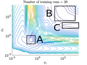
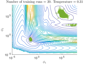
To train the emulator, 20 design points were chosen using Latin hypercube sampling (LHS). For testing purposes, 100 independent design points were chosen by a second LHS. Figure 1(a) shows the multi- modal integrated log-posterior for a fully-parametrised Gaussian process (Garbuno-Inigo et al., 2015). Region A contains a mode with no preference for any dimension. Regions B and C depict different asymptotic behaviours of the emulator. In region B, the emulator behaves as linear regression model, as noted by Andrianakis and Challenor (2012). Region C corresponds to a model which disregards the first dimension. In Figure 1(b) a set of samples obtained by applying TA²S² is showed, illustrating the ability to overcome possible multi-modal distributions that arise in Bayesian analysis of expensive computer codes.

((a)) Level curves

((b)) TA²S² samples

Figure 1: Projection of the negative log-posterior curves in the two dimensional length-scale space for Franke’s simulator using a fully-parametrised Gaussian process. The minimum possible value of $10^{-12}$ for the nugget $\boldsymbol{\phi}_{\delta}$ has been used for the projection and the temperature has been let to reach a practical zero, thus retrieving samples from the modes.

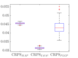
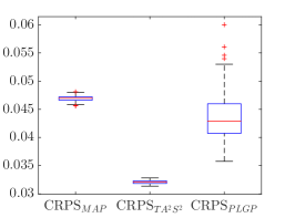
To contrast the proposed sampler against the PLGP benchmark, a set of 100 experiments were run. In each experiment, a sample of size 100 of length-scale hyper-parameters was obtained by each method. This sample size was achieved by thinning the TA²S² results when a chain of length 2000 was constructed in every annealing level. The quality of the probability statements made from both results were compared by means of the CRPS, as depicted in Figure 2. Note that the training set was the same for each experiment and variations in the results among experiments are mainly because of the stochastic nature of the sampling schemes. In Figure 2(a) the boxplots for the CRPS computed from the samples are shown. Figure 2(b) shows the same plots but with an exponential prior for all hyper-parameters with rate 0.2, i.e. $\lambda=5$. This choice of a prior distribution was made since the PLGP software assumes an exponential prior for both the length-scales and nugget term (Gramacy and Polson, 2009). In both settings, the proposed sampler outperforms both the PLGP alternative and the MAP estimate. The latter was calculated from the samples generated by TA²S². Our experiments demonstrated that the MAP estimated this way usually corresponds to the one found by local optimisation routines such as Nelder-Meade or BFGS. The variation in the scores of the MAP illustrates the multi-modality properties of the integrated posterior. All the MAP estimates reported in the remainder are calculated based on this observation. Additionally, it can be seen that the PLGP results seem to contain those achieved by the most probable candidate. In this experiment either using a sample from PLGP or MAP translate in comparable results.

((a)) Reference prior.

((b)) Exponential prior, $\lambda=5.$

Figure 2: Boxplots of CRPS comparing MAP, TA²S² and PLGP. In both cases the proposed sampler outperforms PLGP.

5.2 Nilson-Kuusk model

This simulator models the reflectance of a homogeneous plant canopy. Its five-dimensional input space includes the solar zenith angle, the leaf area index, the relative leaf size, the Markov clumping parameter and a model parameter $\lambda$ (see Nilson and Kuusk, 1989, for further details on the model itself and the meaning of the inputs and output). For the analysis presented in this paper, a single output emulator is assumed and the set of the inputs have been rescaled to fit the hyper-rectangle $[0,1]^{5}$ as in Bastos and O’Hagan (2009).

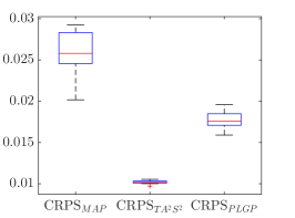
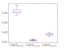
In this experiment, both samplers were used to train a Gaussian process emulator with a dataset of 100 simulation runs. The test set consisted of a different set of 150 training runs. Both datasets, whose design points were generated through LHS, were obtained from the GEM-SA software web page (http://ctcd.group.shef.ac.uk/gem.html). On average, a total of 10 tempered distributions were used in the annealing schedule, while keeping the sampling as $N=5000$ in each level. A thinned sample of 100 experiments was recovered by the end of each TA²S² run to compare results.

The results shown in Figure 3 demonstrate again the overall improved performance of using the proposed sampler in contrast with the benchmark. In this case, one set of experiments (50 iterations) consisted on making inference with the reference prior discussed previously, while the second set (50 iterations) used a common exponential prior. Both samplers outperform the MAP estimate which provides evidence that a more complete uncertainty analysis can be carried out if instead one turns to a full Bayesian inference scheme. Additionally, it is worth noting that Figures 3(a) and 3(b) show that the MAP changes with the prior used. This is not a matter of concern, as it is consistent with the notion that small amount of data is being used for inference and the probabilistic model of the observables is not dominating the prior beliefs.

((a)) Reference prior.

((b)) Exponential prior, $\lambda=5$.

((c)) Sample from TA²S² for each length-scale.

Figure 3: Nilson-Kuusk results obtained after 50 experiments were run. The scatter plot (3(c)) is drawn from a single experiment, in black the MAP estimates.

5.3 Wing weight model

This simulator of the weight of the wing of a light aircraft (Forrester et al., 2008) has been used for input screening. Coupled with a Gaussian process emulator with the squared exponential kernel in equation (2.3), a sensitivity analysis of the wing weight with respect to each input variable can be performed. The model is given by

$$f(\mathbf{x})=0.036\,S_{w}^{0.758}\,W_{fw}^{0.0035}\,\left(\frac{A}{\cos^{2}(\Lambda)}\right)^{0.6}\,q^{0.006}\,\lambda^{0.04}\,\left(\frac{100\,t_{c}}{\cos(\Lambda)}\right)^{-0.3}(N_{z}\,W_{dg})^{0.49}\,+\,S_{w}\,W_{p},$$ (5.6)

where the input variables and the range of their values are summarised in Table 1. For this problem, the evaluation of the reference prior is prohibitive since it scales with the number of dimensions (Paulo, 2005). Thus, a uniform prior in the hyper-parameters’ log-space has instead been used for this experiment.

Input	Range	Description
$S_{w}$	$[150,200]$	Wing area
$W_{fw}$	$[220,300]$	Weight of fuel in the wing
$A$	$[6,10]$	Aspect ratio
$\Lambda$	$[-10,10]$	Quarter-chord sweep
$q$	$[16,45]$	Dynamic pressure at cruise
$\lambda$	$[0.5,1]$	Taper ratio
$t_{c}$	$[0.08,0.18]$	Aerofoil thickness to chord ratio
$N_{z}$	$[2.5,6]$	Ultimate load factor
$W_{dg}$	$[1700,2500]$	Flight design gross weight
$W_{p}$	$[0.025,0.08]$	Paint weight

Table 1: Inputs of the wing weight model.

The inputs were rescaled to the 10-dimensional unit hypercube $[0,1]^{10}$. Two LHS samples of size 100 and 300 were chosen as training and testing sets respectively. At each annealing level, 5000 samples were generated, achieving convergence after 15 levels on average. As before, a thinned sample of 100 was kept to compare results with the benchmark in each experiment. A total of 50 experiments we run in this case.

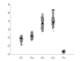
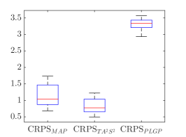
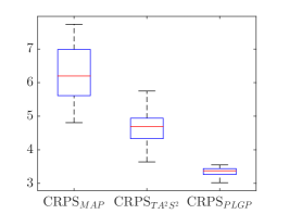
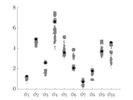
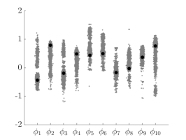
In Figures 4(a) and 4(b), it can be noted that by using sampling one can obtain an improved version of the probabilistic statements made by the surrogate. Figure 4(a) shows that the proposed sampler outperforms the benchmark, concentrating its samples around the mode of the posterior distribution. This is shown by the location and spread of the CRPS for both TA²S² and MAP results, which are similar. Although the CRPS with TA²S² exhibits better performance as can been seen from the location and spread of the boxplot. PLGP in the case of Uniform priors seem to be sampling from other areas with less spread than that of the proposed algorithm. However, if an exponential prior distribution is used for both length-scales and nugget, Figure 4(b), TA²S² is outperformed by the benchmark. Note how the location of the mode changes dramatically, showed by both the means of the boxplot of the CRPS of the MAP, and by the difference of the samples plotted in Figures 4(c) and 4(d). Nonetheless, the proposed sampler is capable of offering improved probabilistic statements for the regression task compared to the MAP estimate.

((a)) Uniform prior.

((b)) Exponential prior, $\lambda=5$.

((c)) Sample from TA²S² for each dimension. Uniform prior.

((d)) Sample from TA²S² for each dimension. Exponential prior.

Figure 4: Results for the wing-weight model using the TA²S² and PLGP algorithms. The scatter plot (3(c)) is drawn from a single experiment, in black the MAP estimates.

6 Conclusions

This paper proposes a method, Transitional Annealed Adaptive Slice Sampling (TA²S²), to sample from the posterior distribution of the Gaussian process’ hyper-parameters. This is known to be a problem where multi-modal distributions are encountered. TA²S² combines Slice Sampling for delayed- rejection, Transitional Markov Chain Monte Carlo (TMCMC) for efficient parallelisation and Markov chain growth, and Asymptotically Independent Markov Sampling (AIMS) for driving the annealing schedule. The delayed-rejection feature of Slice Sampling provides improved mixing which is desirable in highly correlated spaces. Additionally, the proposed algorithm provides a sampling scheme with no burn-in periods for Markov the chain, since each sample generated follows the desired distribution. This is advantageous in Gaussian process applications where the computational burden of the sampling scheme is dominated by the inversion of the correlation matrix. Moreover, efficient coverage of the sampling space is achieved by annealing and an extension of Slice Sampling to Sequential Monte Carlo.

The examples presented show how the method is capable of efficiently exploring multi-modal distributions providing a better alternative to MAP estimates or traditional MCMC methods for Gaussian processes applications. Furthermore, TA²S² allows the generation of samples more efficiently than in traditional MCMC applications, where longer chains are needed to ensure good coverage of the sampling space. This is particularly relevant in the context of computer experiments and Engineering, where it is usually considered that the cost of marginalising the hyper-parameters does not justify the additional computational burden. The proposed method justifies the cost of sampling the hyper-parameters by providing robust estimates of the predicted error. This is reflected through the continuously ranked probability score (CRPS) which shows that the marginalised emulator outperforms MAP estimates. Moreover, the proposed sampling scheme performs as good as the PLGP benchmark, which justifies the annealing by means of functional tempering rather than by subsets of data, which is also sensitive to data permutations.

The proposed algorithm could also be employed for global optimisation problems, by allowing the temperature reach a practical zero. This has application in other areas of Bayesian inference problems and machine learning. As discussed previously, the algorithm can be used in active learning schedules by means of Bayes’ Theorem.

The computational cost of the proposed sampler is dominated by the inversion of the covariance matrix in the integrated posterior distribution. This limitation is inherent to any MCMC schedule used for Gaussian processes. Further strategies to improve the speed of the sampler could be developed, such as the exact evaluation of the log-posterior for candidates where the probability of acceptance is high. For such strategy, a first order Taylor expansion of the objective function could be a feasible enhancement. This is material for future research.

References

- Andrianakis and Challenor (2012) I. Andrianakis and P. G. Challenor. The effect of the nugget on Gaussian process emulators of computer models. Computational Statistics and Data Analysis, 56(12):4215–4228, 2012.
- Andrianakis and Challenor (2011) Y. Andrianakis and P. G. Challenor. Parameter estimation for Gaussian process emulators. Technical report, Managing Uncertainty in Complex Models, 2011.
- Andrieu et al. (2010) C. Andrieu, A. Doucet, and R. Holenstein. Particle Markov chain Monte Carlo methods. Journal of the Royal Statistical Society. Series B: Statistical Methodology, 72(3):269–342, 2010.
- Bastos and O’Hagan (2009) L. S. Bastos and A. O’Hagan. Diagnostics for Gaussian process emulators. Technometrics, 51(4):425–438, 2009.
- Beck and Zuev (2013) J. Beck and K. M. Zuev. Asymptotically Independent Markov Sampling: a new MCMC scheme for Bayesian Inference. International Journal for Uncertainty Quantification, 3(5), 2013.
- Berger and Bernardo (1992) J. O. Berger and J. M. Bernardo. On the development of reference priors. Bayesian Statistics, 4(4), 1992.
- Berger et al. (2009) J. O. Berger, J. M. Bernardo, and D. Sun. The formal definition of reference priors. Annals of Statistics, 37(2):905–938, 2009.
- Birge and Polson (2012) J. R. Birge and N. G. Polson. Optimisation via Slice Sampling. pages 1–22, 2012.
- Ching and Chen (2007) J. Ching and Y.-C. Chen. Transitional Markov Chain Monte Carlo method for Bayesian model updating, model class selection and model averaging. Journal of Engineering Mechanics, 133(7):816–832, 2007.
- Cressie (1993) N. Cressie. Statistics for Spatial Data. Wiley Series in Probability and Statistics. Wiley, 1993.
- De Oliveira (2007) V. De Oliveira. Objective Bayesian analysis of spatial data with measurement error. Canadian Journal of Statistics, 35(2):283–301, 2007.
- Del Moral and Jasra (2007) P. Del Moral and A. Jasra. Sequential Monte Carlo for Bayesian Computation. Bayesian Statistics, 8:1–34, 2007.
- Del Moral et al. (2006) P. Del Moral, A. Doucet, and A. Jasra. Sequential Monte Carlo samplers. Journal of the Royal Statistical Society B, 68(3):411–436, 2006.
- Del Moral et al. (2012) P. Del Moral, A. Doucet, and A. Jasra. On adaptive resampling strategies for sequential Monte Carlo methods. Bernoulli, 18(1):252–278, 2012.
- den Hertog et al. (2006) D. den Hertog, J. P. Kleijnen, and A. Siem. The correct Kriging variance estimated by bootstrapping. Journal of the Operational Research Society, 57(4):400– 409, 2006.
- DiazDelaO and Adhikari (2011) F. DiazDelaO and S. Adhikari. Gaussian process emulators for the stochastic finite element method. International Journal for Numerical Methods in Engineering, 87(6):521–540, 2011.
- Draper (1995) D. Draper. Assessment and propagation of model uncertainty. Journal of the Royal Statistical Society, Series B, 57(1):45–97, 1995.
- Fearnhead and Taylor (2013) P. Fearnhead and B. M. Taylor. An adaptive sequential Monte Carlo sampler. Bayesian Analysis, 8(2):411–438, 2013.
- Forrester et al. (2008) A. I. J. Forrester, A. Sóbester, and A. J. Keane. Engineering Design via Surrogate Modelling. 2008.
- Garbuno-Inigo et al. (2015) A. Garbuno-Inigo, F. A. DiazDelaO, and K. M. Zuev. Gaussian process hyper-parameter estimation using parallel asymptotically independent Markov sampling. Arxiv pre-print, 2015.
- Gelman et al. (1996) A. Gelman, G. Roberts, and W. Gilks. Efficient metropolis jumping rules, 1996.
- Gibbs (1998) M. N. Gibbs. Bayesian Gaussian processes for regression and classification. PhD thesis, Citeseer, 1998.
- Gramacy and Polson (2009) R. B. Gramacy and N. G. Polson. Particle learning of Gaussian process models for sequential design and optimization. Journal Of Computational And Graphical Statistics, 20(1):18, 2009.
- Grimit et al. (2006) E. P. Grimit, T. Gneiting, V. J. Berrocal, and N. a. Johnson. The continuous ranked probability score for circular variables and its application to mesoscale forecast ensemble verification. Quarterly Journal of the Royal Meteorological Society, 132(621C):2925–2942, 2006.
- Haaland and Qian (2012) B. Haaland and P. Z. Qian. Accurate emulators for large-scale computer experiments. Ann. Stat., 39(arXiv: 1203.2433):2974–3002, 2012.
- Hankin (2005) R. Hankin. Introducing BACCO, an R bundle for Bayesian analysis of computer code output. Journal of Statistical Software, 14(16), 2005.
- Kalaitzis and Lawrence (2011) A. A. Kalaitzis and N. D. Lawrence. A simple approach to ranking differentially expressed gene expression time courses through Gaussian process regression. BMC bioinformatics, 12:180, Jan. 2011.
- Katafygiotis and Zuev (2007) L. Katafygiotis and K. Zuev. Estimation of small failure probabilities in high dimensions by adaptive linked importance sampling. In ECCOMAS thematic conference, pages 1–12, 2007.
- Kennedy and O’Hagan (2001a) M. C. Kennedy and A. O’Hagan. Bayesian calibration of computer models. Journal of the Royal Statistical Society: Series B (Statistical Methodology), 63(3):425–464, Aug. 2001a.
- Kennedy and O’Hagan (2001b) M. C. Kennedy and A. O’Hagan. Supplementary details on Bayesian Calibration of Computer Models. Technical report, 2001b.
- Kohonen and Suomela (2006) J. Kohonen and J. Suomela. Lessons learned in the challenge: Making predictions and scoring them. Lecture Notes in Computer Science (including subseries Lecture Notes in Artificial Intelligence and Lecture Notes in Bioinformatics), 3944 LNAI:95–116, 2006.
- MacKay (1998) D. J. MacKay. Introduction to Monte Carlo methods. In Learning in graphical models, pages 175–204. Springer, 1998.
- MacKay (1996) D. J. C. MacKay. Hyperparameters: Optimize, or integrate out? Maximum entropy and Bayesian methods, pages 43–59, 1996.
- Murray and Adams (2010) I. Murray and R. P. Adams. Slice sampling covariance hyperparameters of latent Gaussian models. 2(1):9, 2010.
- Murray et al. (2009) I. Murray, R. P. Adams, and D. J. C. Mackay. Elliptical slice sampling. (2), 2009.
- Neal (1993) R. M. Neal. Probabilistic inference using Markov Chain Monte Carlo methods. Technical Report, pages 1–144, 1993.
- Neal (1997) R. M. Neal. Monte Carlo implementation of Gaussian process models for Bayesian regression and classification. Technical Report 9702, 1997.
- Neal (1998) R. M. Neal. Regression and classification using Gaussian process priors. Bayesian Statistics, 6, 1998.
- Neal (2001) R. M. Neal. Annealed importance sampling. Statistics and Computing, 11(2):125–139, 2001.
- Neal (2003) R. M. Neal. Slice sampling. Annals of Statistics, 31(3), 2003.
- Neal (2011) R. M. Neal. MCMC using Hamiltonian dynamics. In Handbook of Markov Chain Monte Carlo. 2011.
- Nilson and Kuusk (1989) T. Nilson and A. Kuusk. A reflectance model for the homogeneous plant canopy and its inversion. Remote Sensing of Environment, 27(2):157–167, 1989.
- Nocedal and Wright (2004) J. Nocedal and S. J. Wright. Numerical Optimization. Springer, 2004.
- Oakley (1999) J. Oakley. Bayesian Uncertainty Analysis for Complex Computer Codes. PhD thesis, 1999.
- Oakley (2002) J. Oakley. Eliciting Gaussian process priors for complex computer codes. Journal of the Royal Statistical Society Series D: The Statistician, 51(1):81–97, 2002.
- Paulo (2005) R. Paulo. Default priors for Gaussian processes. Annals of Statistics, 33(2):556–582, 2005.
- Ranjan et al. (2011) P. Ranjan, R. Haynes, and R. Karsten. A computationally stable approach to Gaussian process interpolation of deterministic computer simulation data. Technometrics, 53(4):366–378, 2011.
- Rasmussen and Williams (2006) C. E. Rasmussen and C. K. I. Williams. Gaussian Processes for Machine Learning. MIT Press, 2006.
- Taflanidis and Beck (2008a) A. A. Taflanidis and J. L. Beck. Stochastic Subset Optimization for optimal reliability problems. Probabilistic Engineering Mechanics, 23(2-3):324–338, Apr. 2008a.
- Taflanidis and Beck (2008b) A. A. Taflanidis and J. L. Beck. An efficient framework for optimal robust stochastic system design using stochastic simulation. Computer Methods in Applied Mechanics and Engineering, 198(1):88–101, 2008b.
- Vernon et al. (2010) I. Vernon, M. Goldstein, and R. G. Bower. Galaxy formation: a Bayesian uncertainty analysis. Bayesian Analysis, 5(4):619–669, Dec. 2010. j
- Warnes and Ripley (1987) J. J. Warnes and B. D. Ripley. Problems with likelihood Estimation of Covariance Function of Spatial Gaussian Processes. Biometrika, 74(3):640–642, 1987.
- Wilkinson (2014) R. D. Wilkinson. Accelerating ABC methods using Gaussian processes. arXiv preprint, 2014.
- Williams and Rasmussen (1996) C. K. I. Williams and C. E. Rasmussen. Gaussian processes for regression. Advances in Neural Information Processing Systems, pages 514–520, 1996.
- Zuev and Beck (2013) K. M. Zuev and J. L. Beck. Global optimization using the Asymptotically Independent Markov Sampling method. Computers & Structures, 126:107–119, Sept. 2013.