Domain structure; hysteresis Finite-size systems Numerical simulation; solution of equations

Multidomain switching in the ferroelectric nanodots

Abstract

Controlling the polarization switching in the ferroelectric nanocrystals, nanowires and nanodots has an inherent specificity related to the emergence of depolarization field that is associated with the spontaneous polarization. This field splits the finite-size ferroelectric sample into polarization domains. Here, based on 3D numerical simulations, we study the formation of 180^∘ polarization domains in a nanoplatelet, made of uniaxial ferroelectric material, and show that in addition to the polarized monodomain state, the multidomain structures, notably of stripe and cylindrical shapes, can arise and compete during the switching process. The multibit switching protocol between these configurations may be realized by temperature and field variations.

A fundamental property of ferroelectrics is the interplay between the spontaneous polarization, $\mathbf{P}$, appearing due to the symmetry-breaking off-center displacement of polar ions, and the long-range depolarization electric field caused by the same polarization. The depolarization field is induced by depolarizing charges distributed with volume density $\rho=\mathrm{div}\mathbf{P}$ in regions where the polarization is nonuniform and with surface charge density $\sigma=\mathbf{Pn}$ in the near-surface layer of polarization termination points (here, $\mathbf{n}=\left(n_{x},n_{y},n_{z}\right)$ is the unit vector, normal to the sample surface and directed outside the sample). As illustrated in Fig. 1a for the finite-size sample, the depolarization field is distributed in the inner space and in the surrounding outer space that costs an additional electrostatic energy and impedes the formation of the ferroelectric state.

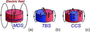
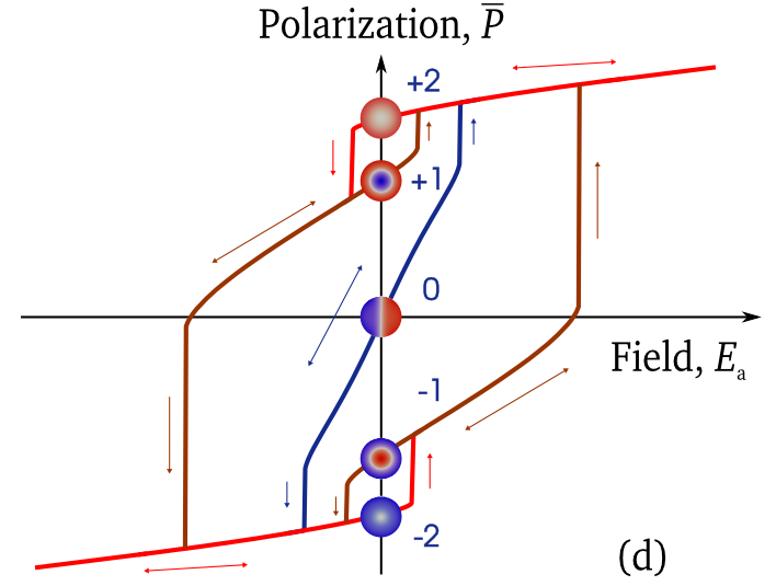
Figure 1: Distribution of the depolarization electric field in the ferroelectric nadodot (ND) with the polarized monodomain state, MDS (a), the two-band state, TBS (b), and the concentric-cylindrical state, CCS (c). Panel (d) shows the multibit switching between these states, denoted by quantum numbers $0$, $\pm 1$ and $\pm 2$. The red and blue colors correspond to the ”up” and ”down” polarization orientations.

The tendency to reduce the unfavorable action of the depolarization field was noted by Landau and Kittel more than 60 years ago [1, 2, 3] as able to lead to a polarization domain patterning of the sample. As shown in Figs. 1bc, the formation of the oppositely polarized 180^∘ domains alternates the associated depolarizing charge at the surface. This confines the depolarization field closer to the surface, diminishing its energy. The price for the gain however is the additional cost of domain wall (DW) creation. Hence, the domain form and size are the result of a tiny balance between geometry, electrostatic and ferroelectric properties of the system. Figs. 1bc exemplify the competition between the stripe and cylindric domain patterns. The situation becomes even more delicate if an external field is applied. The interaction with the field changes the domain configuration, favoring the ”up”-oriented domains with polarization parallel to the field. The growth of the up-polarized domains continues up to complete poling of the sample to the monodomain state.

The formation of Landau-Kittel domains having the structure of regular periodic stripes in thin ferroelectric films was studied over the past decade both experimentally [4, 5, 6, 7] and theoretically [8, 9, 10, 11]. The period of the domain pattern was found to scale according to the Landau-Kittel square root law as [8, 12, 13]

$$2d\simeq 2\sqrt{3.53\,\left(\widetilde{\varepsilon}/\varepsilon_{c}\right)\text{ }\xi_{0}h},$$ (1)

where $h$ is the film thickness, $\xi_{0}\simeq 1\,\mathrm{nm}$ is the atomic-scale coherence length, $\widetilde{\varepsilon}=\varepsilon_{p}+\left(\varepsilon_{c}\varepsilon_{a}\right)^{1/2}$, $\varepsilon_{c}$ and $\varepsilon_{a}$ are the intrinsic longitudinal and transversal (to polarization and to stripes) dielectric constants of the ferroelectric state and $\varepsilon_{p}$ is the dielectric constant of the surrounding paraelectric environment. When the electric field, $E_{a}$, is applied, the theoretical calculations predict the stretching of up-oriented domains and the contraction of down-oriented domains. Interestingly, this induces the oppositely-oriented coarse-grained depolarization field that finally leads to the negative permittivity of the ferroelectric layer [14, 15]. The behavior of the domain structure at higher fields is little studied although one can guess that the oppositely-oriented domain stripes will transform to the vanishing domain droplets before the complete polarization of the system, similarly as it happens in ferromagnetic samples [16, 17]. Recent numerical calculations for ferroelectric films [18] confirm this hypothesis.

Much less is known concerning the properties of the Landau-Kittel 180^∘ domains in finite-scale nanodot (ND) samples, with sizes comparable to the predicted domain width $d$. Meanwhile, it is the application of the NDs that is considered to be very promising in the emerging ferroelectric-based nanoelectronics for the realization of high-density memory-storage units [13]. The experimental [19, 20, 21] and theoretical [22, 23, 24, 25] efforts were mostly concentrated on the pseudo-cubic perovskite ferroelectrics with eight possible polarization orientations. The diversity of domains and of polarization-vortex patterns was discovered, but the systematic study was partially impeded by the complexity of the system. The electrostatic depolarization effects are strongly coupled with ferroelastic ones, produced by the polarization rotations and by the strain of the near-surface dead layer [26].

In this letter we study how the Landau-Kittel structure of 180^∘ polarization domains is formed in a finite-size sample. We show that the confining electrostatic effects result in the various domain structures. Field and temperature applications permit to realize the controllable multibit switching between them, hence increasing the volume of the writable information per ND.

To disjoint the depolarization effects, that are primary for the domain formation, from the secondary lattice-deformation effects, we consider the uniaxial ferroelectric material for which the ferroelastic coupling is small. To be specific, we select the Sodium Nitrite, NaNO₂,  as model material. It has the orthorhombic symmetry, hence only two, ”up” and ”down”, orientations of the spontaneous polarization $P_{0}\simeq 12~{}\mathrm{\mu C/cm}^{2}$ with respect to the $c$-axis. The anisotropic tensor of dielectric constants has the principal values $\varepsilon_{a}\simeq 10$, $\varepsilon_{b}\simeq 5$ and $\varepsilon_{c}\simeq 12$ at low temperatures [27, 28], providing the preferred orientation of DW in the $bc$-plane.

The ferroelectric transition in the bulk NaNO₂ crystal occurs at $T_{c}\simeq 433\,\mathrm{K}$, the Curie constant, $C$, being equal to $5000\,\mathrm{K\ }$[27]. The characteristic value of the depolarization field is estimated as $E_{0}=P_{0}/\varepsilon_{0}\simeq 13.5\times 10^{4}\,\mathrm{kV/cm}$ (here $\varepsilon_{0}$ is the vacuum permittivity). We assume also that the crystal is cut in the form of cylindrical nanoplatelet of radius $r\simeq 8\,\mathrm{nm}$ and of thickness $h\simeq 1.7\,\mathrm{nm}$, the spontaneous polarization being directed along the cylinder axis. The ND is embedded into the dielectric matrix with $\varepsilon_{p}\simeq 90$. The high value of $\varepsilon_{p}$ is required to reduce the depolarization energy. Otherwise the depolarization effects will kill the ferroelectric phase, even in the multidomain state. With such a selection of parameters, the characteristic domain width, calculated according to Eq. (1), is $d\simeq 7.1\,\mathrm{nm}$ that is commensurate with the ND radius, $r$.

The principal results are illustrated in Fig. 1. At zero applied field the ND can stay either in the polarized monodomain state (MDS), Fig. 1a, or in one of the multidomain states. The competition occurs mostly between the two-band state (TBS), Fig. 1b,  and the concentric-cylindrical state (CCS), Fig. 1c, although other configurations are also possible. The average polarization of the TBS, $\overline{P}$, is zero whereas the CCS and the MDS have the nonzero polarizations, either “up”-oriented or ”down”-oriented. We ascribe the appropriate quantum numbers, $N=0,$ $\pm 1$ and $\pm 2$, to the TBS, CCS and MDS respectively, where the sign reflects the orientation of $\overline{P}$.

The field application allows to jump among the TBS, CCS and MDS as sketched in Fig. 1d. Usually, the TBS arises at zero-field cooling. When the field, $E_{a}>0$, is applied the TBS stays reversibly-stable until it jumps to the up-oriented MDS. Further field increase and reversal cycling produce the hysteresis curve that, depending on the field variation protocol, realizes the four-bit switching between the CCS with $N=\pm 1$ and the MDS with $N=\pm 2$. Although the initial TBS with $N=0$ is no longer accessible, it can again be achieved by ”thermal reboot” consisting in the heating of the system to the paraelectric state with subsequent zero-field cooling.  The interplay between the TBS and the CCS during the ND poling is a legacy of the already mentioned field-induced transition between stripe and droplet domain configurations in an infinite system.

An analogous multiple-hysteresis phenomenon was recently observed in mesoparticles of superconducting lead and explained by an irreversible decay of magnetic vortex droplets [29]. The effect was shown to be similar to the Rayleigh fragmentation of a charged liquid due to the competition between the long-range Coulomb charge repulsion and the short-range molecular attraction [30]. The buckling, faceting, or even disintegration of ferroelectric domains also can be driven by the long-range repulsion between DWs, associated with the electric fringing fields of depolarization charges [31].

To give the further insight on the switching process we describe the methodology of calculations. We consider the nonuniform Ginzburg-Landau equation for the order parameter, spontaneous polarization $P$, coupled with the electrostatic equation for the electric potential $\varphi_{f}$, in $\Omega_{f}$, the interior of the ND, [10, 11]:

$$\left(t+\frac{P^{2}}{P_{0}^{2}}-\xi_{0a}^{2}\partial_{x}^{2}-\xi_{0b}^{2}\partial_{y}^{2}-\xi_{0c}^{2}\partial_{z}^{2}\right)P=-\varepsilon_{0}\kappa_{c}\partial_{z}\varphi_{f},$$

$$\varepsilon_{0}\left(\varepsilon_{a}\partial_{x}^{2}+\varepsilon_{b}\partial_{y}^{2}+\varepsilon_{ic}\partial_{z}^{2}\right)\varphi_{f}=\partial_{z}P.$$ (2)

Here, $t=(T-T_{c})/T_{c}$ is the reduced temperature, $\kappa_{c}=C/T_{c}\simeq 11.5$ is the displacive parameter [32], $\varepsilon_{ic}\gtrsim 1$ is the small nonpolar contribution to the Curie-Weiss divergency of $\varepsilon_{c}$, such as $\varepsilon_{c}(t)=\varepsilon_{ic}+\kappa_{c}/t$ at $T\gtrsim T_{c}$. The coordinates $x$, $y$ and $z$ are selected along the axes $a$, $b$ and $c$, the corresponding coherence lengths $\xi_{0a}$, $\xi_{0b}$ and $\xi_{0c}$ are roughly equal to $1\,\mathrm{nm}$. To catch the generic features of the switching we use the simplistic cubic form of the nonlinear term, digressing from the more specific details of the transition. The parameter $P_{0}$  is selected as spontaneous polarization at low temperatures. The electric field and the electric displacement are given by $\mathbf{E}_{f}=-\nabla\varphi_{f}$ and $\mathbf{D}_{f}=\varepsilon_{0}\mathbf{E}_{f}+\mathbf{P}_{f}$, where the components of the polarization vector, $\mathbf{P}_{f}$, are written as: $P_{f,x}=\varepsilon_{0}\left(\varepsilon_{a}-1\right)E_{f,x}$, $P_{f,y}=\varepsilon_{0}\left(\varepsilon_{b}-1\right)E_{f,y}$ and $P_{f,z}=\varepsilon_{0}\left(\varepsilon_{ic}-1\right)E_{f,z}+P$.

The relations (2) are completed by the Poisson equation $\nabla^{2}\varphi_{p}=0$ for the electric potential $\varphi_{p}$, outside the ND. The corresponding electric field and displacement are expressed as $\mathbf{E}_{p}=-\nabla\varphi_{p}$ and $\mathbf{D}_{p}=\varepsilon_{0}\varepsilon_{p}\mathbf{E}_{p}$.

Electrostatic rules imply the continuity of the potential, $\varphi_{f}=\varphi_{p}$, and of the normal component of the electric displacement, $\mathbf{D}_{f}\mathbf{n}=\mathbf{D}_{p}\mathbf{n}$. In our notation, the latter constraint is written as $\varepsilon_{0}\varepsilon_{ic}\mathbf{\partial}_{z}\varphi_{f}-P=\varepsilon_{0}\varepsilon_{p}\mathbf{\partial}_{z}\varphi_{p}$ for the upper and lower ND surfaces and as $\left(\varepsilon_{a}n_{x}\partial_{x}+\varepsilon_{b}n_{y}\partial_{y}\right)\varphi_{f}=\varepsilon_{p}\left(n_{x}\partial_{x}+n_{y}\partial_{y}\right)\varphi_{p}$ for the lateral surface. For the polarization we took the free boundary condition $\left(\xi_{0a}^{2}n_{x}\partial_{x}+\xi_{0b}^{2}n_{y}\partial_{y}+\xi_{0c}^{2}n_{z}\partial_{z}\right)P=0$ at the sample surface.

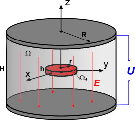
Figure 2: Geometrical parameters of the system.

The calculation setup is shown in Fig. 2. To model the outer potential distribution, the ND was embedded into a bigger space, $\Omega$, with sufficiently large volume to avoid to disturb the emergent fringing field. In practice the cylinder with radius $R\simeq 12\,\mathrm{nm}$ and thickness $H\simeq 17\,\mathrm{nm}$ was taken, the independence of the obtained results on the cylinder sizes was checked at each calculation stage. The potential difference $\Delta\varphi_{p}=U$ between the top and bottom electrodes was applied to induce the field $E_{a}=U/H$, the variation of $\varphi_{p}$ at the lateral surface being assumed to be linear, $\varphi_{p}(z)=(z/H)U$.

We deal then with the boundary value problem satisfied by $P$ and $\varphi$, where the electric potential in $\Omega$ is denoted by $\varphi$, as being $\varphi_{f}$ or $\varphi_{p}$, namely inside or outside the ND. The approach for solving numerically this 3D problem is based on a finite element method, implemented as Fortran 90 homemade code (see [33] for details). First, we introduced a variational formulation of the problem, for which the variational unknowns, representing $P$ and $\varphi$, are found in the Sobolev spaces $H^{1}(\Omega_{f})$ and $H^{1}(\Omega)$ respectively [34]. Then, we discretized this formulation by making use of a mesh of $\overline{\Omega}$ (the closure of $\Omega$) and of the Lagrange finite elements of the first order. This mesh consists of a collection of tetrahedra, obtained from a usual process of triangulation, and is fine enough near the boundaries of $\Omega_{f}$ and $\Omega$. The discrete regions associated with $\overline{\Omega_{f}}$ and $\overline{\Omega}$ are polyhedral. In a correlative way, the discrete region associated with the boundary of $\Omega_{f}$ is entirely made up of faces of tetrahedra. Each of these faces is common both to a tetrahedron of the discrete region associated with $\overline{\Omega_{f}}$ and another one of the discrete region associated with $\overline{\Omega_{p}}=\overline{\Omega\setminus\Omega_{f}}$. By dealing with a mesh size equal to $0.47\,\mathrm{nm}$ for $\overline{\Omega_{f}}$ and to $0.61\,\mathrm{nm}$ for $\overline{\Omega_{p}}$, we were led to a square nonlinear system of $485621$ scalar equations. Let us mention that this system is not subject to a uniqueness of solution, as it is the case for the associated discrete and continuous variational formulations. Finally, we solved the system with the help of an inexact Newton method [35], combined at each iteration with the Generalized Minimal RESidual (GMRES) algorithm [36]; a preconditioner, based on an incomplete LU factorization (see, e.g., [37]), was incorporated into this algorithm.

We systematically dealt with the initialization of the inexact Newton method either with a randomly generated datum or with a solution profile obtained at the previous calculations. The behavior of the system as a function of the temperature or of the field was followed with the step of at most $10^{-2}$ of the running interval whereas the finer step of $10^{-3}$ was used in the points of the brutal solution changes.

Eqs. (2) were also studied in [38] for the ellipsoidal ND of triglicine sulfate (TGS), having similar dielectric properties. In particular the temperature-induced CCS-MDS transition was observed. However, only the axially-symmetric domain profiles (that are not always the most stable) were obtained. For instance, the steady TBS was overlooked. This does not permit to see all the diversity of the possible domain structures and to investigate the field-induced switching between them, that is the subject of the current article.

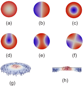
Figure 3: (a)-(f) Different (meta)-stable polarization profiles, obtained from random initial polarization distributions. Lower panel shows the polarization distribution in the CCS for the equatorial (g) and vertical (h) sections of the ND.

In what follows, we start from study of temperature evolution of the system and show that the different metastable domain states can be formed at the same temperature; some of them are presented in Fig. 3. To catch all the possible states, we simulated the zero-field thermal quenching to low temperatures. Random polarization and random potential were taken at the initialization stage. Then, the final converging state was registered. Repeating the numerical experiment with different initial distributions, we found that, in addition to the already mentioned MDS, TBS and CCS (Figs. 3a-c, respectively), other profiles, like the asymmetric-droplet state (Fig. 3d) and the three-band state (Fig. 3e), can arise at $T=0$. Several other domain patterns were also seen, but on a less regular basis. In the TBS, the polarizations of up- and down-oriented domains are compensated, giving $\overline{P}=0$. In other states the average polarization is nonzero; the latter being maximal in the MDS.

To follow the temperature evolution of the observed domain states we performed the adiabatic heating when the next-on-heating state was obtained from the previous one, taking the latter as the initial configuration. The average spontaneous polarization of each of the discovered states decreases on heating (see Fig. 4), each state having its own temperature range of existence above which it irreversibly jumps to another one, more enduring state. The corresponding transition temperature was identified as the temperature of superheating. Remarkably, no jump corresponding to a supercooling instability was observed on adiabatic cooling.

The MDS  stays stable on heating till  the temperature $0.18T_{c}$, above which it suddenly jumps to the CCS. The asymmetric-droplet state also transforms to the CCS  by almost continuous coalescence of the edge-connecting neck but at higher temperature, $0.62T_{c}$. The average polarization of the CCS itself gradually decreases and at $0.63T_{c}$ the system transforms to the TBS.

The TBS is the most enduring state. Its average polarization is always zero, whereas the maximal domain polarization also decreases on heating and vanishes at $T_{0}=0.68T_{c}$. This temperature can be considered as the ferroelectric transition temperature of the ND.  As concerns the three-band state, it remains metastable till $0.37T_{c}$. Then, it transforms to the new diamond-like state (Fig. 3f) with $\overline{P}=0$, which at $0.65T_{c}$ drops to the TBS.

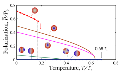
Figure 4: Temperature evolution of the average polarization of the ND for different domain configurations. Dots denote the most stable state. The polarization is given in units of the zero-temperature bulk spontaneous polarization, $P_{0}$, the temperature is given in units of the bulk critical temperature, $T_{c}$.

We identified the most stable domain configuration at each temperature, calculating the free energy, $F=-\frac{1}{4\kappa_{c}P_{0}^{2}}\int P^{4}d\Omega$ [11], for each state (see the dot marks in Fig. 4). The TBS remains the most stable on cooling from $T_{0}$ to $0.17T_{c}$ and then, the avail in energy passes to the MDS (see dashed line in Fig. 4). This thermodynamic transition temperature is slightly lower than the given above superheating temperature for the MDS, $0.18T_{c}$.

Figure 5: Hysteresis curves for different domain states at $T=0.1T_{c}$. The average polarization of the ND is given in units of the spontaneous polarization, $P_{0}$ at $T=0$, the applied electric field is given in units of the bulk depolarization field $E_{0}=P_{0}/\varepsilon_{0}$.

Figs. 3gh illustrate the polarization distribution inside the CCS at low temperatures. The width of the DW is of the order of $4$-$6\,\xi_{0}$ which is larger than the typical atomistic DW width in bulk materials. The DW has Ising-like structure when the polarization changes in amplitude, across the wall, but stays almost parallel to the $\mathbf{z}$-axis. At higher temperatures the DW profile becomes even softer [10, 11]. There is also no substantial change in the polarization value when passing across the ND from bottom to top. This makes a difference with the high-$\varepsilon$ perovskite ferroelectrics, where the polarization flux-closure at termination points of the DW has been observed [9, 12, 11]. The determining difference is in the opposite ratio $\varepsilon_{p}/\varepsilon_{c}$ that substantially reduces the depolarization effects in the embedded ND of NaNO₂. Another striking feature we observed is the deviation of DWs from the most preferable $bc$-plane, clearly seen in the diamont-like structure (Fig. 3f), and also the DWs buckling in the three-band state and, especially, in the asymmetric-droplet state. We believe that this effect is provided by the already mentioned interplay between the positive DW tension energy and the negative nonlocal electrostatic energy of the fringing field [29].

The behavior of the multidomain structures in external field was also studied by a similar method of adiabatic field variation. Fig. 5 (which is the extended version of Fig. 1d) presents the hysteresis loops, $\overline{P}(E_{a})$, for various domain states at $T=0.1T_{c}$. Monitoring the domain evolution in the applied field gives more insight into dynamics of the switching process. Starting from the zero-field cooled TBS, having $\overline{P}=0$, and gradually increasing the field, we follow the central (blue) branch of the hysteresis loop. We notice that the DW in the TBS starts to bend, to diminish the unfavorable polarization. At some threshold field it irreversibly escapes from the sample to form the up-polarized MDS, which is the most stable state at $E_{a}\geq 0$. The MDS remains with further field increase, forming the upper (red) branch of the hysteresis loop. Backward field decrease keeps the MDS till $E_{a}=0$  and even further, for small negative $E_{a}$, when the up-polarized MDS turns to be metastable with respect to the down-polarized MDS.

Polarization distribution in the MDS is nonuniform. Feedback action of the depolarization field reduces the spontaneous polarization closer to the centers of the ND circular plane surfaces, the effect known as Landau-Lifshitz branching [2]. Such a polarization central sagging becomes especially pronounced when the field downturns below zero. Finally, the polarization suddenly flips at the central part of the ND with formation of the (metastable) CCS. Notably, the average polarization of the just formed CCS is smaller than that in the original MDS but is still up-oriented, that is against the applied field.

Further evolution of the system, shown by the brown line, depends on the protocol of the field cycling. While the down-oriented field continues to grow, the relative volume of the internal negatively-polarized cylindrical domain also increases. At some critical field, that is nothing but the coercive field of the system, the internal domain suddenly expands to the whole volume with the formation of the stable down-polarized MDS. This accomplishes the semi-loop of the global hysteresis, that can be completed by its centrally-symmetric counterpart under the rearward field sweep. If, however, right after the MDS$\rightarrow$CCS switching, the running of the applied field reverses from the decrease to the increase, the internal domain diminishes and, at some threshold $E_{a}>0$, suddenly vanishes to restore the original MDS. This closes the local hysteresis loop that can be observed between the MDS and CDS at small field oscillations.

The evolution of the three-band and asymmetric-droplet domain states in the applied field (green and magenta lines in Fig. 5, respectively) can be characterized as a ”repulsive cycling”. Once these configurations are formed by the thermal quenching, they can live durably in their metastable state and be locally-stable under small field variation. However, in larger fields, they become unstable with respect to transition to the more regular TBS, CCS or MDS.  As soon as this happens, there is no way to restore the original state back neither via the temperature nor via the field variation. They disappear very soon after the regular high-amplitude field cycling. For instance, one of the bent DWs of the three-band state escapes on the field variation and the system jumps to the TBS. Note the unusual crossing of the green and blue branches of the hysteresis curve, implying that $\overline{P}$ is not a unique function of $E_{a}$ but depends also on the domain configuration.

The behavior of the asymmetric-droplet state is even more diverse. Depending on the direction of the field variation, it can either join the CCS, similar as in the temperature diagram in Fig. 4, or jump to the TBS or to the MDS. The first case occurs when approaching the coercive field in which the system drops immediately to the oppositely-polarized MDS state. In the second case the accidental bifurcation degeneracy with respect to selection of the switching trajectory was observed. Within the temperature-induced fluctuation incertitude both the transitions to the TBS or to the MDS can occur (see dashed magenta line in Fig 5). The interesting feature of the transition to the TBS is the lowering of $\overline{P}$ when the applied field increases.

The observed variety of nanoscale domain states with their irreversible history-dependent evolution can elucidate the dynamics of the relaxor materials that, at certain conditions, can be viewed as a set of interacting polarization nanoclusters with intrinsic domain structure, similar to the ferroelectric NDs. Parameters of our model system were selected in a special way to highlight the controlled five-bit switching. Modifications of the ND geometry and of dielectric properties of the material can lead to the realization of other domain configurations with topologically different hysteresis loops and even with a higher number of switching bits.

To conclude, we performed the complete analysis of the domains formation and of the hysteresis switching process in the uniaxial ferroelectric ND as a function of the temperature and of the applied field. Various stable and metastable domain states were found. The most remarkable among them, the TBS, CCS and MDS, can be formed in a controlled way, during the regular zero-field cooling and systematic variation of the applied field. This paves the way to the predictable individual domain manipulation on the nanoscale. The discovered multibit switching opens new routes for the design of high-capacity nanosize memory-storage devices in the ferroelectric-based nanoelectronics.

References

- [1] LANDAU L. D. and LIFSHITZ E. M., Phys. Z. Sowjetunion, 8 (1935) 153.
- [2] LANDAU L. D. and LIFSHITZ E. M., Electrodynamics of Continuous Media (Elsevier, New York, 1985).
- [3] KITTEL C., Phys. Rev., 70 (1946) 965.
- [4] STREIFFER S. K., EASTMAN J. A., FONG D. D. et al., Phys. Rev. Lett., 89 (2002) 067601.
- [5] ZUBKO P., STUCKI N., LICHTENSTEIGER C. and TRISCONE J.-M., Phys. Rev. Lett., 104 (2010) 187601.
- [6] ZUBKO P., JECKLIN N., TORRES-PARDO A. et al., Nano Lett., 12 (2012) 2846.
- [7] HRUSZKEWYCZ S. O., HIGHLAND M. J., HOLT M. V. et al., Phys. Rev. Lett., 110 (2013) 177601.
- [8] BRATKOVSKY A. M. and LEVANYUK A. P., Phys. Rev. Lett., 84 (2000) 3177.
- [9] KORNEV I., FU H. and BELLAICHE L., Phys. Rev. Lett., 93 (2004) 196104.
- [10] STEPHANOVICH V. A., LUK’YANCHUK I. A. and KARKUT M. G., Phys. Rev. Lett., 94 (2005) 047601.
- [11] LUK’YANCHUK I. A., LAHOCHE L. and SENÉ A., Phys. Rev. Lett., 102 (2009) 147601.
- [12] DE GUERVILLE F., LUK’YANCHUK I., LAHOCHE L. and EL MARSSI M., Mater. Sci. Eng. B, 120 (2005) 16.
- [13] CATALAN G., SEIDEL J., RAMESH R. and SCOTT J. F., Rev. Mod. Phys., 84 (2012) 119.
- [14] BRATKOVSKY A. M. and LEVANYUK A. P., Phys. Rev. B, 63 (2001) 132103.
- [15] LUK’YANCHUK I., PAKHOMOV A., SIDORKIN A. and VINOKUR V., arXiv:1410.3124 (2014).
- [16] CAPE J. A. and LEHMAN G. W., J. Appl. Phys., 42 (1971) 5732.
- [17] MALOZEMOFF A. P. and SLONCZEWSKI J. C., Magnetic domain walls in bubble materials, Academic Press, 1979.
- [18] ARTEMEV A., Phil. Mag., 90 (2010) 89.
- [19] TIEDKE S., SCHMITZ T., PRUME K.et al, Appl. Phys. Lett., 79 (2001) 3678.
- [20] SCHILLING, A., BYRNE D., CATALAN, G. Nano Lett. 9 (2009) 3359.
- [21] AHLUWALIA R., NG N., SCHILLING A. et al., Phys. Rev. Lett., 111 (2013) 165702.
- [22] MÜNCH I., HUBER J. E., Appl. Phys. Lett., 95 (2009) 022913.
- [23] WANG J., Appl. Phys. Lett. 97 (2010) 192901.
- [24] WU, C. M., CHEN W. J., ZHENG Y., et al., Scientific reports 4 (2014) 3946.
- [25] STEPKOVA V., MARTON P., SETTER N. and HLINKA J., Phys. Rev. B, 89 (2014) 060101.
- [26] LUK’YANCHUK I. A., SCHILLING A., GREGG J. M., CATALAN G., and SCOTT J. F., Phys. Rev. B, 79 (2009) 144111.
- [27] SHIOZAKI Y., NAKAMURA E. and MITSUI T. (Eds.), Ferroelectrics and Related Substances: Oxides Part 1: Perovskite-type Oxides and LiNbO3 Family, Landolt-Börnstein: Numerical Data and Functional Relationships in Science and Technology - New Series III/36A1 / Condensed Matter, 2001.
- [28] Our selection of axes , , and corresponds to crystallographic axes , and in NaNO2, see [27].
- [29] LUK’YANCHUK I., VINOKUR V. M., RYDH A. et al., Nature. Phys., 11 (2015) 21.
- [30] RAYLEIGH, LORD, FRS, Philosophical Magazine, Series 5, 14:87 (1882) 184.
- [31] LUKYANCHUK I., SHARMA P., NAKAJIMA T. et al., Nano Lett., 14 (2014) 6931.
- [32] STRUKOV B. A. and LEVANYUK, A. P., Ferroelectric phenomena in crystals: physical foundations. Springer Science & Business Media, 2012.
- [33] MARTELLI P.-W., Ph. D. Thesis, University of Lorraine, in preparation.
- [34] ADAMS R. A., Sobolev Spaces, Academic Press, New York, 1975.
- [35] DENNIS JR. J. E and SCHNABEL R. B., Numerical methods for unconstrained optimization and nonlinear equations, Vol. 16. SIAM, 1996.
- [36] SAAD Y. and SCHULTZ M. H., SIAM J. Sci. Stat. Comput., 7 (1986) 856.
- [37] QUARTERONI A., SACCO R. and SALERI F., Numerical mathematics, Vol. 37, Springer-Verlag, NY, 2000.
- [38] NECHAEV V. N. and VISKOVATYKH A. V., Phys. Solid State, 57 (2015) 722.