The central limit theorem for a sequence of random processes with space varying long memory

Abstract

In this paper we investigate a sequence of square integrable random processes with space varying memory. We establish sufficient conditions for the central limit theorem in the space $L^{2}(\mu)$ for the partial sums of the sequence of random processes with space varying long memory. Of particular interest is a non-standard normalization of the partial sums in the central limit theorem.

Keywords: long memory, random processes, square integrable sample paths, central limit theorem, weak convergence.

MSC: 60F05, 60B12.

1 Introduction

Memory of a second-order stationary sequence of random variables $\left\{Y_{k}\right\}$ is usually defined in terms of the decay of autocovariances $\operatorname{Cov}\left[Y_{0},Y_{h}\right]$. For example, $\left\{Y_{k}\right\}$ is said to have long memory if the series

$$\sum_{h=0}^{\infty}\left\lvert\operatorname{Cov}\left[Y_{0},Y_{h}\right]\right\rvert$$

diverges, while short memory of $\left\{Y_{k}\right\}$ corresponds to the convergence of the series above. For a review of the notion of long memory, we refer to Samorodnitsky [11]; for probabilistic foundations, statistical methods, and applications, we refer to Giraitis, Koul, and Surgailis [4], and Beran [1].

Interesting and important features of memory are reflected in the growth rate of the partial sums $\sum_{k=1}^{n}Y_{k}$. The partial sums $\sum_{k=1}^{n}Y_{k}$ of a short memory sequence of random variables appear to grow at the rate of the central limit theorem $n^{1/2}$, whereas the partial sums of a long memory sequence of random variables may grow faster. For example, if $\operatorname{Cov}\left[Y_{0},Y_{h}\right]\sim h^{-d},0<d<1$, then the partial sums $\sum_{k=1}^{n}Y_{k}$ grow at the rate of $n^{1-d/2}$.

Memory of a sequence of multidimensional random elements may vary in space. That is, it can depend on the direction the sequence is projected. Memory of a second-order stationary sequence of Hilbert space valued random elements $\left\{Y_{k}\right\}$ can be associated with the regular decay of the autocovariance operators $Q_{h}\mathrel{\mathop{:}}=\operatorname{Cov}\left[Y_{0},Y_{h}\right]$ by assuming, for instance, $Q_{h}\sim h^{-D}Q$, where $D$ and $Q$ are certain operators on the Hilbert space (see Račkauskas and Suquet [10] for further details). The corresponding sequence has space varying memory which depends on the operator $D$.

We investigate a sequence of random processes $\left\{X_{k}\right\}\mathrel{\mathop{:}}=\left\{X_{k}(t),t\in S\right\}$ which is defined for each $k\in\mathbb{Z}$ and each $t\in S$ by

$$X_{k}(t)\mathrel{\mathop{:}}=\sum_{j=0}^{\infty}\left(j+1\right)^{-d(t)}\varepsilon_{k-j}(t),$$

where $S$ is some index set, $\left\{\varepsilon_{k}(t)\right\}$ is a sequence of independent and identically distributed random variables and $d(t)$ is a real function of $t$.

The sequence $\left\{X_{k}(t)\right\}$ for each $t\in S$ is essentially similar to the fractional ARIMA$\left(0,1-d(t),0\right)$ process, which may be expressed as an MA$\left(\infty\right)$ process with the coefficients

$$\frac{\Gamma\left(j+1-d(t)\right)}{\Gamma\left(j+1\right)\Gamma\left(1-d(t)\right)},\quad j=0,1,2\ldots,$$

where $\Gamma(\cdot)$ is the gamma function (the fractional ARIMA process was introduced by Granger and Joyeux [5] and Hosking [7]). The application of Stirling’s formula to the coefficients above yields the following relation:

$$\frac{\Gamma\left(j+1-d(t)\right)}{\Gamma\left(j+1\right)\Gamma\left(1-d(t)\right)}\sim\frac{j^{-d(t)}}{\Gamma\left(1-d(t)\right)}\quad\text{as}\quad j\to\infty.$$

The growth rate of the partial sums $\sum_{k=1}^{n}X_{k}(t)$ depends on $t$. Interpreting $k\in\mathbb{Z}$ as a time index and $t\in S$ as a space index we thus have a sequence of real valued random processes $\left\{X_{k}\right\}=\left\{X_{k}(t),t\in S\right\}$ with space varying memory. Such sequences of random processes could serve as a model in functional data analysis (we refer to Ramsay and Silverman [9] for an introduction to functional data analysis, for the theory of linear processes in function spaces, see Bosq [2]).

We investigate the growth of the partial sums $\sum_{k=1}^{n}X_{k}$ in the sample path space of square integrable real valued functions and establish sufficient conditions for the central limit theorem for the partial sums $\sum_{k=1}^{n}X_{k}$.

Figure 1 shows simulated sample paths of the random processes of the sequence $\left\{X_{k}\right\}$. The sequence $\left\{\varepsilon_{k}\right\}\mathrel{\mathop{:}}=\left\{\varepsilon_{k}(t):t\in[0,1]\right\}$ was assumed to be a sequence of independent and identically distributed standard Wiener processes on the interval $[0,1]$ and the function $d:[0,1]\to(1/2,+\infty)$ was assumed to be a step function $d(t)=d_{1}\chi_{[0,1/2)}(t)+d_{2}\chi_{[1/2,1]}(t)$, where $\chi_{A}$ is the indicator function of $A$. The simulated sample paths for $5$ consecutive elements of the sequence $\left\{X_{k}\right\}$ were plotted. The procedure was completed for two different sets of the values of $d_{1}$ and $d_{2}$ ($d_{1}=0.6,d_{2}=2$ and $d_{1}=0.6,d_{2}=0.7$).

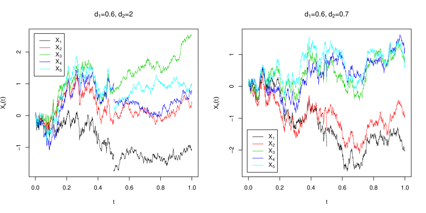
Figure 1: Simulated sample paths of the random processes of the sequence $\left\{X_{k}\right\}$ (horizontal axis is the index set $[0,1]$ of the random processes $\left\{X_{k}\right\}$, vertical axis is the value of the random process $X_{k}(t)$ at a point $t\in[0,1]$)

The rest of the paper is organized as follows. The sequence of random processes $\left\{X_{k}\right\}$ is defined and investigated in Section 2. In Section 3 we establish sufficient conditions for the central limit theorem for the partial sums $\sum_{k=1}^{n}X_{k}$.

2 Some preliminaries

Let $(S,\mathcal{S},\mu)$ be a $\sigma$-finite measure space. Consider a sequence of independent and identically distributed measurable random processes $\left\{\varepsilon_{k}\right\}\mathrel{\mathop{:}}=\left\{\varepsilon_{k}(t):t\in S\right\}$ defined on the same probability space $\left(\Omega,\mathcal{F},P\right)$ with $\operatorname{E}\varepsilon_{k}(t)=0$ and $\operatorname{E}\varepsilon_{k}^{2}(t)<\infty$ for each $t\in S$ and each $k\in\mathbb{Z}$. Let us denote $\sigma^{2}(t)\mathrel{\mathop{:}}=\operatorname{E}\varepsilon_{0}^{2}(t)$ and $\sigma(s,t)\mathrel{\mathop{:}}=\operatorname{E}\left[\varepsilon_{0}(s)\varepsilon_{0}(t)\right]$, where $s,t\in S$.

We define a sequence of random processes $\left\{X_{k}\right\}\mathrel{\mathop{:}}=\left\{X_{k}(t),t\in S\right\}$ by setting for each $t\in S$ and each $k\in\mathbb{Z}$

$$X_{k}(t)\mathrel{\mathop{:}}=\sum_{j=0}^{\infty}\left(j+1\right)^{-d(t)}\varepsilon_{k-j}(t),$$ (1)

where $d(t)>1/2$ for each $t\in S$. $d(t)>1/2$ is a necessary and sufficient condition for the almost sure convergence of the series (1). This fact easily follows from Kolmogorov’s three-series theorem.

It is possible to choose some other second-order stationary sequence of random variables that can have long memory (for example, $Y_{k}(t)=\sum_{j=0}^{\infty}a_{j}(t)\varepsilon_{k-j}(t)$, where $a_{j}(t)\sim(j+1)^{-d(t)}$), but our aim is to investigate space varying memory and we want to avoid any unnecessary technical difficulties.

If $\operatorname{E}\varepsilon_{0}(t)\neq 0$, then the sequence $\left\{X_{k}(t)\right\}$, $t\in S$, can only have short memory (i.e. absolutely summable autocovariances), since then the series (1) converges almost surely if and only if $d(t)>1$ and absolute summability of $\left(j+1\right)^{-d(t)}$ implies that autocovariances are absolutely summable (see, for example, Hamilton [6], p. 70).

Routine calculations show that the sequences $\left\{X_{k}(s)\right\}$ and $\left\{X_{k}(t)\right\}$ for $s,t\in S$ are sequences of zero mean random variables with the following expression for the cross-covariance

$$\operatorname{E}\left[X_{0}(s)X_{h}(t)\right]=\sigma(s,t)\sum_{j=0}^{\infty}\left(j+1\right)^{-d(s)}\left(j+h+1\right)^{-d(t)}.$$ (2)

Now we establish the asymptotic behaviour of the sequence of cross-covariances. $a_{n}\sim b_{n}$ as $n\to\infty$ indicates that the sequences $a_{n}$ and $b_{n}$ are asymptotically equivalent, i.e. the ratio of the two sequences tends to one as $n$ goes to infinity.

Proposition 1.

Let $s,t\in S$ be fixed. If $1/2<d(s)<1$ and $d(t)>1/2$, then

$$\operatorname{E}\left[X_{0}(s)X_{h}(t)\right]\sim c(s,t)\sigma(s,t)\cdot h^{1-\left[d(s)+d(t)\right]}\quad\text{as}\quad h\to\infty,$$

where

$$c(s,t)\mathrel{\mathop{:}}=\int_{0}^{\infty}\!x^{-d(s)}(x+1)^{-d(t)}\,\mathrm{d}x.$$ (3)

If $s=t$, we denote $c(t)\mathrel{\mathop{:}}=c(t,t)$ and $\sigma^{2}(t)\mathrel{\mathop{:}}=\sigma(t,t)$.

If $d(s)=d(t)=1$, then

$$\operatorname{E}\left[X_{0}(s)X_{h}(t)\right]\sim\sigma(s,t)\cdot h^{-1}\ln h\quad\text{as}\quad h\to\infty.$$

Proof.

We approximate the series in equation (2) by integrals to obtain the following inequalities: if $\frac{1}{2}<d(s)<1$ and $d(t)>\frac{1}{2}$, then we obtain

$$\sum_{j=0}^{\infty}\left(j+1\right)^{-d(s)}\left(j+h+1\right)^{-d(t)} \geq h^{1-\left[d(s)+d(t)\right]}\int_{\frac{1}{h}}^{\infty}\!x^{-d(s)}\left(x+1\right)^{-d(t)}\,\mathrm{d}x,$$ (4)

$$\sum_{j=0}^{\infty}\left(j+1\right)^{-d(s)}\left(j+h+1\right)^{-d(t)} \leq h^{1-\left[d(s)+d(t)\right]}\int_{0}^{\infty}\!x^{-d(s)}\left(x+1\right)^{-d(t)}\,\mathrm{d}x;$$

if $d(s)=d(t)=1$, then we have that

$$\sum_{j=0}^{\infty}\left[(j+1)(j+h+1)\right]^{-1} \geq h^{-1}\left[\ln\left(\frac{h+1}{2}\right)+\int_{1}^{\infty}\![y(y+1)]^{-1}\,\mathrm{d}y\right]$$

$$\sum_{j=0}^{\infty}\left[(j+1)(j+h+1)\right]^{-1} \leq\left(h+1\right)^{-1}+h^{-1}\left[\ln\left(\frac{h+1}{2}\right)+\int_{1}^{\infty}\!\left[y(y+1)\right]^{-1}\,\mathrm{d}y\right].\qed$$

Next, we investigate the convergence of the series of cross-covariances.

Proposition 2.

Let $s,t\in S$. The series

$$\sum_{h=1}^{\infty}\operatorname{E}\left[X_{0}(s)X_{h}(t)\right]$$ (5)

converges if and only if both of the conditions $d(t)>1$ and $d(s)+d(t)>2$ are fulfilled.

Proof.

Series (5) has the following expression

$$\sum_{h=1}^{\infty}\operatorname{E}\left[X_{0}(s)X_{h}(t)\right]=\sigma(s,t)\left[\sum_{h=1}^{\infty}\left(h+1\right)^{-d(t)}+\sum_{h=1}^{\infty}\sum_{j=1}^{\infty}\left(j+1\right)^{-d(s)}\left(j+h+1\right)^{-d(t)}\right].$$

The first series of the right-hand side of the equation above converges if and only if $d(t)>1$. Thus, we only need to investigate the convergence of the series

$$\sum_{h=1}^{\infty}\sum_{j=1}^{\infty}\left(j+1\right)^{-d(s)}\left(j+h+1\right)^{-d(t)}.$$ (6)

A slight modification of inequality (4) shows that series (6) diverges if $d(s)+d(t)\leq 2$. To show that series (6) converges if $d(t)>1$ and $d(s)+d(t)>2$, we choose $\delta>0$ such that $1<1+\delta<d(t)$ and $d(s)+d(t)-\delta>2$ to obtain the following inequality

$$\sum_{h=1}^{\infty}\sum_{j=1}^{\infty}\left(j+1\right)^{-d(s)}\left(j+h+1\right)^{-d(t)}\leq\sum_{h=1}^{\infty}\sum_{j=1}^{\infty}\left(j+1\right)^{-d(s)-d(t)+1+\delta}h^{-(1+\delta)}<\infty.\qed$$

Remark 1.

The series $\sum_{h=1}^{\infty}\operatorname{E}\left[X_{0}(t)X_{h}(t)\right]$ converges if and only if $d(t)>1$.

Suppose $\mathcal{L}^{2}\left(\mu\right)\mathrel{\mathop{:}}=\mathcal{L}^{2}\left(S,\mathcal{S},\mu\right)$ is a separable space of real valued square $\mu$-integrable functions with a seminorm

$$\left\|f\right\|_{2}\mathrel{\mathop{:}}=\left(\int_{S}\!\left\lvert f(r)\right\rvert^{2}\,\mu\left(\mathrm{d}r\right)\right)^{1/2}.$$

Proposition 3 establishes assumptions under which the sample paths of the processes $\left\{X_{k}\right\}$ almost surely belong to the space $\mathcal{L}^{2}\left(\mu\right)$.

Proposition 3.

The sample paths of the random processes $\left\{X_{k}\right\}$ almost surely belong to the space $\mathcal{L}^{2}\left(\mu\right)$ if and only if both of the integrals

$$\quad\int_{S}\!\sigma^{2}(r)\,\mu(\mathrm{d}r)\quad\text{and}\quad\int_{S}\!\frac{\sigma^{2}(r)}{2d(r)-1}\,\mu(\mathrm{d}r)$$ (7)

are finite.

Proof.

We show that the expected value

$$\operatorname{E}\left[\int_{S}\,X^{2}_{0}\left(r\right)\!\mu\left(\mathrm{d}r\right)\right]$$

is finite if and only if integrals (7) are finite. First, using Fubini’s theorem we obtain

$$\operatorname{E}\left[\int_{S}\,X^{2}_{0}\left(r\right)\!\mu\left(\mathrm{d}r\right)\right]=\int_{S}\,\operatorname{E}X^{2}_{0}\left(r\right)\!\mu\left(\mathrm{d}r\right).$$

Secondly, setting $h=0$ and $s=t$ in equation (2) gives the expression for the variance

$$\operatorname{E}X_{0}^{2}(t)=\sigma^{2}(t)\sum_{j=0}^{\infty}\left(j+1\right)^{-2d(t)},\quad t\in S.$$

Approximation of the series above by integrals leads to the following inequalities

$$2\int_{S}\!\operatorname{E}X_{0}^{2}(r)\,\mu\left(\mathrm{d}r\right) \geq\int_{S}\!\sigma^{2}(r)\,\mu\left(\mathrm{d}r\right)+\int_{S}\!\frac{\sigma^{2}(r)}{2d(r)-1}\,\mu\left(\mathrm{d}r\right),$$

$$\int_{S}\!\operatorname{E}X_{0}^{2}(r)\,\mu\left(\mathrm{d}r\right) \leq\int_{S}\!\sigma^{2}(r)\,\mu\left(\mathrm{d}r\right)+\int_{S}\!\frac{\sigma^{2}(r)}{2d(r)-1}\,\mu\left(\mathrm{d}r\right).\qed$$

3 The central limit theorem

Before we formulate sufficient conditions for the central limit theorem, we clarify what is meant by weak convergence of a sequence of random processes with square $\mu$-integrable sample paths (see Cremers and Kadelka [3] for details). Suppose $\left\{\xi_{n}\right\}$ is a sequence of measurable random processes with sample paths in $\mathcal{L}^{2}\left(\mu\right)$. Let $L^{2}\left(\mu\right)\mathrel{\mathop{:}}=L^{2}\left(S,\mathcal{S},\mu\right)$ be the corresponding Banach space of equivalence classes of $\mu$-almost everywhere equal measurable functions and let $\mathcal{B}\left(L^{2}\left(\mu\right)\right)$ be its Borel $\sigma$-algebra. The maps $\hat{\xi}_{n}:\Omega\to L^{2}\left(\mu\right),\omega\to\hat{\xi}_{n}(\omega)\mathrel{\mathop{:}}=\xi_{n}\left(\omega,\cdot\right)$ are $\mathcal{F}-\mathcal{B}\left(L^{2}\left(\mu\right)\right)$-measurable (see Cremers and Kadelka [3]); hence the distributions $\hat{P}_{n}$ of $\hat{\xi}_{n}$ are well defined probability measures on $\left(L^{2}\left(\mu\right),\mathcal{B}\left(L^{2}\left(\mu\right)\right)\right)$. It is said that the sequence $\left\{\xi_{n}\right\}$ converges weakly to $\xi$ and it is written $\xi_{n}\Rightarrow\xi$ if the corresponding image measures $\hat{P}_{n}$ converge weakly, i.e. $\int f\mathrm{d}\hat{P}_{n}\to\int f\mathrm{d}\hat{P}$ for all continuous and bounded real valued functions defined on $L^{2}\left(\mu\right)$.

The following result establishes sufficient conditions for the central limit theorem for the partial sums $\sum_{k=1}^{n}X_{k}$.

Proposition 4.

1. Suppose $1/2<d(t)<1$, $\operatorname{E}\varepsilon_{0}^{2}(t)<\infty$ for each $t\in S$ and both of the integrals

   $$\int_{S}\!\frac{\sigma^{2}(r)}{\left[1-d(r)\right]^{2}}\,\mu\left(\mathrm{d}r\right)\quad\text{and}\quad\int_{S}\!\frac{\sigma^{2}(r)}{\left[1-d(r)\right]\left[2d(r)-1\right]}\,\mu\left(\mathrm{d}r\right)$$ (8)

   are finite. Then

   $$n^{-H}\sum_{k=1}^{n}X_{k}\Rightarrow\mathcal{G},$$

   where $n^{-H}$ is a sequence of multiplication operators with the expression $n^{-H}f(t)=n^{-\left[3/2-d(t)\right]}f(t)$ for each $t\in S$, $f\in L^{2}\left(\mu\right)$, and $\mathcal{G}\mathrel{\mathop{:}}=\left\{\mathcal{G}(t),t\in S\right\}$ is a zero mean Gaussian random process with the following autocovariance function

   $$\operatorname{E}\left[\mathcal{G}(s)\mathcal{G}(t)\right]=\frac{\left[c(s,t)+c(t,s)\right]\sigma(s,t)}{\left(2-\left[d(s)+d(t)\right]\right)\left(3-\left[d(s)+d(t)\right]\right)},$$

   where $c(s,t)$ is the function (3) and $\sigma(s,t)\mathrel{\mathop{:}}=\operatorname{E}\left[\varepsilon_{0}(s)\varepsilon_{0}(t)\right]$, $s,t\in S$.

2. Suppose $d(t)=1$ and $\operatorname{E}\varepsilon_{0}^{2}(t)<\infty$ for each $t\in S$ and

   $$\int_{S}\!\sigma^{2}(r)\,\mu\left(\mathrm{d}r\right)<\infty.$$

   Then

   $$\frac{1}{\sqrt{n}\ln n}\sum_{k=1}^{n}X_{k}\Rightarrow\mathcal{G}^{\prime},$$

   where $\mathcal{G^{\prime}}\mathrel{\mathop{:}}=\left\{\mathcal{G^{\prime}}(t),t\in S\right\}$ is a zero mean Gaussian random process with the autocovariance function $\operatorname{E}\left[\mathcal{G}^{\prime}(s)\mathcal{G}^{\prime}(t)\right]=\sigma(s,t)$, where $\sigma(s,t)\mathrel{\mathop{:}}=\operatorname{E}\left[\varepsilon_{0}(s)\varepsilon_{0}(t)\right],s,t\in S$.

Remark 2.

If the essential infimum of $d\left(t\right)$ is greater than 1, that is, if

$$\sup\left\{x\in\mathbb{R}:\mu\left(\left\{t:d\left(t\right)<x\right\}\right)=0\right\}>1,$$

then we can use Theorem 1 of Račkauskas and Suquet [8] to show that the central limit theorem holds for the partial sums of a similar second-order stationary sequence of $L^{2}\left(\mu\right)$-valued random elements. Suppose that $\left\{\psi_{k}\right\}$ is a sequence of independent and identically distributed random elements of $L^{2}\left(\mu\right)$. Let us define a sequence of $L^{2}\left(\mu\right)$-valued random elements by setting for each $k\in\mathbb{Z}$

$$Y_{k}\mathrel{\mathop{:}}=\sum_{j=0}^{\infty}A_{j}\psi_{k-j},$$ (9)

where $A_{j}$ is a sequence of multiplication operators with the following expression

$$A_{j}\psi_{k-j}\left(t\right)=\left(j+1\right)^{-d(t)}\psi_{k-j}(t)$$

for each $t\in S$. The sequence (9) is essentially similar to the sequence $\left\{X_{k}\right\}$ of random processes (1). According to Theorem 1 of Račkauskas and Suquet [8], $n^{-1/2}\sum_{k=1}^{n}Y_{k}$ converges in distribution to a Gaussian random element of $L^{2}\left(\mu\right)$ if $n^{-1/2}\sum_{k=1}^{n}\psi_{k}$ converges in distribution to a Gaussian random element of $L^{2}\left(\mu\right)$ (see Račkauskas and Suquet [8] for more details).

Proof of Proposition 4.

The proof is based on a part of Theorem 2 of Cremers and Kadelka [3]. We provide the proof in several steps. To establish that the sequence $\left\{\xi_{n}\right\}$ weakly converges to $\xi$, we need to show that the following is true:

1. for each $t\in S$ $\operatorname{E}\xi_{n}^{2}(t)\to\operatorname{E}\xi^{2}(t)$ as $n\to\infty$;

2. the finite-dimensional distributions of $\xi_{n}$ converge weakly to those of the $\xi$ almost everywhere;

3. for each $t\in S$ and $n\in\mathbb{N}$ $\operatorname{E}\xi_{n}^{2}(t)\leq f(t)$, where $f$ is a non-negative $\mu$-integrable function.

We begin by proving part (a). We show that for each $t\in S$ the sequences $\operatorname{E}\left[n^{-\left[3/2-d(t)\right]}\sum_{k=1}^{n}X_{k}(t)\right]^{2}$ and $\operatorname{E}\left[(\sqrt{n}\ln n)^{-1}\sum_{k=1}^{n}X_{k}(t)\right]^{2}$ converge to $\operatorname{E}\mathcal{G}^{2}(t)$ and $\operatorname{E}\mathcal{G}^{\prime 2}(t)$ respectively.

The growth rate of the cross-covariance of the partial sums of the sequences $\left\{X_{k}(s)\right\}$ and $\left\{X_{k}(t)\right\},s,t\in S$, is established in Proposition 5.

Proposition 5.

If $1/2<d(s)<1$ and $1/2<d(t)<1$, then

$$\operatorname{E}\left[\left(\sum_{k=1}^{n}X_{k}(s)\right)\left(\sum_{k=1}^{n}X_{k}(t)\right)\right]\sim\frac{\left[c(s,t)+c(t,s)\right]\sigma(s,t)}{\left(2-\left[d(s)+d(t)\right]\right)\left(3-\left[d(s)+d(t)\right]\right)}\cdot n^{3-\left[d(s)+d(t)\right]}\quad\text{as}\quad n\to\infty,$$

where $c(s,t)$ is function (3).

If $d(s)=1$ and $d(t)=1$, then

$$\operatorname{E}\left[\left(\sum_{k=1}^{n}X_{k}(s)\right)\left(\sum_{k=1}^{n}X_{k}(t)\right)\right]\sim\sigma(s,t)\cdot n\ln^{2}n.$$

Proof.

The cross-covariance of the partial sums of the sequences $\left\{X_{k}(s)\right\}$ and $\left\{X_{k}(t)\right\}$ has the following expression

$$\operatorname{E}\left[\left(\sum_{k=1}^{n}X_{k}(s)\right)\left(\sum_{k=1}^{n}X_{k}(t)\right)\right]=n\operatorname{E}\left[X_{0}(s)X_{0}(t)\right]\\ +\sum_{k=1}^{n-1}\sum_{l=k+1}^{n}\operatorname{E}\left[X_{k}(s)X_{l}(t)\right]+\sum_{k=1}^{n-1}\sum_{l=k+1}^{n}\operatorname{E}\left[X_{k}(t)X_{l}(s)\right].$$ (10)

Since

$$\sum_{k=1}^{n-1}\sum_{l=k+1}^{n}\operatorname{E}\left[X_{k}(s)X_{l}(t)\right]=n\sum_{k=1}^{n-1}\operatorname{E}\left[X_{0}(s)X_{k}(t)\right]-\sum_{k=1}^{n-1}k\operatorname{E}\left[X_{0}(s)X_{k}(t)\right],$$

we can use the results of Proposition 1 to obtain the following asymptotic relations: if $1/2<d(s)<1$ and $1/2<d(t)<1$, then

$$\sum_{k=1}^{n-1}\operatorname{E}\left[X_{0}(s)X_{k}(t)\right] \sim\frac{c(s,t)\sigma(s,t)}{2-\left[d(s)+d(t)\right]}\cdot n^{2-\left[d(s)+d(t)\right]},$$

$$\sum_{k=1}^{n-1}k\operatorname{E}\left[X_{0}(s)X_{k}(t)\right] \sim\frac{c(s,t)\sigma(s,t)}{3-\left[d(s)+d(t)\right]}\cdot n^{3-\left[d(s)+d(t)\right]};$$

if $d(s)=1$ and $d(t)=1$, then

$$\sum_{k=1}^{n-1}\operatorname{E}\left[X_{0}(s)X_{k}(t)\right] \sim\frac{\sigma(s,t)}{2}\cdot\ln^{2}n,$$

$$\sum_{k=1}^{n-1}k\operatorname{E}\left[X_{0}(s)X_{k}(t)\right] \sim\sigma(s,t)\cdot n\ln n.\qed$$

Remark 3.

The growth rate of the variance of the partial sums of the sequence $\left\{X_{k}(t)\right\}$ is the following: if $1/2<d(t)<1$, then

$$\operatorname{E}\left[\sum_{k=1}^{n}X_{k}(t)\right]^{2} \sim\frac{c(t)\sigma^{2}(t)}{\left[1-d(t)\right]\left[3-2d(t)\right]}\cdot n^{3-2d(t)};$$

if $$d(t)=1$$, then

$$\operatorname{E}\left[\sum_{k=1}^{n}X_{k}(t)\right]^{2} \sim\sigma^{2}(t)\cdot n\ln^{2}n.$$

Remark 3 completes the proof of part (a).

Now we move on to the proof of part (b) and show that the finite dimensional distributions of $n^{-H}\sum_{k=1}^{n}X_{k}$ and $(\sqrt{n}\ln n)^{-1}\sum_{k=1}^{n}X_{k}$ converge to those of $\mathcal{G}$ and $\mathcal{G}^{\prime}$ respectively. In order to prove the convergence of finite dimensional distributions we investigate a sequence of random vectors

$$\left(\begin{array}[]{ccc}b_{n}^{-1}(t_{1})\sum_{k=1}^{n}X_{k}(t_{1})&\ldots&b_{n}^{-1}(t_{q})\sum_{k=1}^{n}X_{k}(t_{q})\end{array}\right),$$ (11)

where $t_{1},\ldots,t_{q}\in S$ and

$$b_{n}(t)\mathrel{\mathop{:}}=\begin{cases}n^{3/2-d(t)},&1/2<d(t)<1;\\ \sqrt{n}\ln n,&d(t)=1.\end{cases}$$

The sum of dependent random variables $\sum_{k=1}^{n}X_{k}(t)$ can be expressed as a series of independent random variables: if $n\geq 2$, then we have the following identity

$$\sum_{k=1}^{n}X_{k}(t)=\sum_{j=-\infty}^{n}z_{n,j}(t)\varepsilon_{j}(t),$$

where

$$z_{n,j}(t)\mathrel{\mathop{:}}=\begin{cases}\sum_{k=1}^{n-j+1}k^{-d(t)},&2\leq j\leq n;\\ \sum_{k=1}^{n}\left(k-j+1\right)^{-d(t)},&j<2.\end{cases}$$

By denoting

$$\varepsilon_{j}^{(q)}\mathrel{\mathop{:}}=\left(\begin{array}[]{ccc}\varepsilon_{j}(t_{1})&\ldots&\varepsilon_{j}(t_{q})\end{array}\right)^{\mathrm{T}}$$

and

$$B_{n,j}\mathrel{\mathop{:}}=\operatorname{diag}\left(\begin{array}[]{ccc}b_{n}^{-1}(t_{1})z_{n,j}(t_{1})&\ldots&b_{n}^{-1}(t_{q})z_{n,j}(t_{q})\end{array}\right),$$

we can express the sequence of random vectors (11) compactly as

$$\sum_{j=-\infty}^{n}B_{n,j}\varepsilon_{j}^{(q)}=\left(\begin{array}[]{c}\sum_{j=-\infty}^{n}\left[b_{n}^{-1}(t_{1})z_{n,j}(t_{1})\right]\varepsilon_{j}(t_{1})\\ {1}\\ \sum_{j=-\infty}^{n}\left[b_{n}^{-1}(t_{q})z_{n,j}(t_{q})\right]\varepsilon_{j}(t_{q})\end{array}\right).$$

Using the fact that the operator norm of a diagonal matrix is the largest entry in absolute value, we obtain the operator norm of the matrix $B_{n,j}$

$$\left\|B_{n,j}\right\|_{M}=\max_{1\leq i\leq q}\left\lvert b_{n}^{-1}(t_{i})z_{n,j}(t_{i})\right\rvert.$$

Now suppose that

$$\gamma_{j}^{(q)}\mathrel{\mathop{:}}=\left(\begin{array}[]{ccc}\gamma_{j}(t_{1})&\ldots&\gamma_{j}(t_{q})\end{array}\right)^{\mathrm{T}}$$

is a zero mean normal random vector with the same covariance matrix as the vector $\varepsilon_{j}^{(q)}$. The sequence $\sum_{j=-\infty}^{n}B_{n,j}\gamma_{j}^{(q)}$ converges in distribution to a normal random vector if and only if the sequence of covariance matrices converges. Clearly, it follows from the results of Proposition 5, that the sequence of covariance matrices converges.

To prove that the finite dimensional distributions converge weakly, we apply Proposition 4.1 of Račkauskas and Suquet [10], which establishes that under certain conditions the sequences $\sum_{j=-\infty}^{n}B_{n,j}\varepsilon_{j}^{(q)}$ and $\sum_{j=-\infty}^{n}B_{n,j}\gamma_{j}^{(q)}$ have the same limiting behaviour in the sense that if one converges in distribution then so does the other and their limits coincide.

We consider for $q$-dimensional random vectors $U$ and $V$ the distance

$$\zeta_{3}\left(U,V\right)\mathrel{\mathop{:}}=\sup_{f\in\mathcal{F}_{3}}\left\lvert\operatorname{E}f\left(U\right)-\operatorname{E}f\left(V\right)\right\rvert,$$

where $\mathcal{F}_{3}$ is the set of three times Frechet differentiable functions $f:\mathbb{R}^{q}\to\mathbb{R}$ such that

$$\sup_{x\in\mathbb{R}^{q}}\left\lvert f^{(j)}(x)\right\rvert\leq 1,\quad\text{for}\ j=0,\ldots,3.$$

For the sake of convenience, we state Proposition 4.1 of Račkauskas and Suquet [10] here.

Proposition 6.

If the following two conditions

$$\lim_{n\to\infty}\sup_{j\in\mathbb{Z}}\left\|B_{n,j}\right\|_{M}=0$$ (12)

and

$$\limsup_{n\to\infty}\sum_{j\in\mathbb{Z}}\left\|B_{n,j}\right\|_{M}^{2}<\infty.$$ (13)

are satisfied, then

$$\lim_{n\to\infty}\zeta_{3}\left(\sum_{j=-\infty}^{n}B_{n,j}\varepsilon_{j}^{(q)},\sum_{j=-\infty}^{n}B_{n,j}\gamma_{j}^{(q)}\right)=0.$$

Propositon 7 establishes that the sequence of operator norms of the matrices $B_{n,j}$ satisfies two properties that are needed to apply Proposition 6.

Proposition 7.

If $\frac{1}{2}<d(t)\leq 1$ for each $t\in S$, then both of conditions (12) and (13) are satisfied.

Proof.

To prove that condition (12) holds, we first notice that

$$\sup_{j\in\mathbb{Z}}\left\|B_{n,j}\right\|_{M}=\max_{1\leq i\leq q}\left\lvert b_{n}^{-1}(t_{i})z_{n,1}(t_{i})\right\rvert$$

and then we use the following asymptotic relations: if $\frac{1}{2}<d(t)<1$, then we have that

$$\sum_{k=1}^{n}k^{-d(t)}\sim\frac{n^{1-d(t)}}{1-d(t)};$$

if $d(t)=1$, then we obtain

$$\sum_{k=1}^{n}k^{-1}\sim\ln n.$$

We use the following expression to prove that condition (13) holds

$$\sum_{j=-\infty}^{n}z_{n,j}^{2}(t)=\sum_{j=2}^{n}\left[\sum_{k=1}^{n-j+1}k^{-d(t)}\right]^{2}+\sum_{j=0}^{\infty}\left[\sum_{k=1}^{n}\left(k+j\right)^{-d(t)}\right]^{2}.$$

Routine approximations of sums by integrals from above lead to the following inequalities: if $\frac{1}{2}<d(t)<1$, then we have that

$$\sum_{j=2}^{n}\left[\sum_{k=1}^{n-j+1}k^{-d(t)}\right]^{2}\leq\frac{1}{\left[1-d(t)\right]^{2}[3-2d(t)]}\left[n^{3-2d(t)}-1\right];$$

if $d(t)=1$, then we obtain

$$\sum_{j=2}^{n}\left[\sum_{k=1}^{n-j+1}k^{-1}\right]^{2}\leq(n-1)+n\ln^{2}n.$$

To prove that

$$\lim_{n\to\infty}\frac{1}{n^{3-2d(t)}}\sum_{j=0}^{\infty}\left[\sum_{k=1}^{n}\left(k+j\right)^{-d(t)}\right]^{2}<\infty$$

for $\frac{1}{2}<d(t)\leq 1$, we first divide the series in the expression above into two summands

$$\sum_{j=0}^{\infty}\left[\sum_{k=1}^{n}\left(k+j\right)^{-d(t)}\right]^{2}=\left[\sum_{k=1}^{n}k^{-d(t)}\right]^{2}+\sum_{j=1}^{\infty}\left[\sum_{k=1}^{n}\left(k+j\right)^{-d(t)}\right]^{2}$$ (14)

and approximate the first summand on the right-hand side of the equation (14) by integral from above

$$\sum_{k=1}^{n}k^{-d(t)}\leq\begin{cases}\frac{n^{1-d(t)}}{1-d(t)}&\text{if}\quad\frac{1}{2}<d(t)<1;\\ 1+\ln n&\text{if}\quad d(t)=1.\end{cases}$$

We express the second summand on the right-hand side of equation (14) in the following way

$$\frac{1}{n^{3-2d(t)}}\sum_{j=1}^{\infty}\left[\sum_{k=1}^{n}(k+j)^{-d(t)}\right]^{2}=\sum_{i=1}^{\infty}\frac{1}{n}\sum_{j=(i-1)n+1}^{in}\left[\frac{1}{n}\sum_{k=1}^{n}\left(\frac{k}{n}+\frac{j}{n}\right)^{-d(t)}\right]^{2}$$

and the interchange of limits leads to the result

$$\lim_{n\to\infty}\frac{1}{n^{3-2d(t)}}\sum_{j=1}^{\infty}\left[\sum_{k=1}^{n}(k+j)^{-d(t)}\right]^{2}=\int_{0}^{\infty}\!\left[\int_{0}^{1}\!(s+u)^{-d(t)}\,\mathrm{d}s\right]^{2}\,\mathrm{d}u<\infty.\qed$$

The proof of part (b) is complete.

Finally, we prove part (c). Proposition 8 establishes the existence of non-negative $\mu$-integrable functions that dominate the sequence of the variance of the partial sums.

Proposition 8.

Let $t\in S$. If $\frac{1}{2}<d(t)<1$, then

$$\operatorname{E}\left[\frac{1}{n^{3/2-d(t)}}\sum_{k=1}^{n}X_{k}(t)\right]^{2}\leq\sigma^{2}(t)\left[1+\frac{1}{2d(t)-1}\right]+\frac{\sigma^{2}(t)c(t)}{\left[1-d(t)\right]\left[3-2d(t)\right]},$$ (15)

where $c(t)$ is the function (3). If $d(t)=1$ for each $t\in S$, then

$$\operatorname{E}\left[\frac{1}{\sqrt{n}\ln n}\sum_{k=1}^{n}X_{k}(t)\right]^{2}\leq C\cdot\sigma^{2}(t),$$ (16)

where $C$ is a positive constant.

Proof.

To establish the first inequality in Proposition 8, we set $s=t$ in expression (10) and approximate the sums in expression (10) by integrals from above.

The following reasoning leads to inequality (16). We set $s=t$ in expression $\eqref{eq:pscov}$ to obtain an expression for the left-hand side of inequality (16). Since $d(t)=1$ for each $t\in S$, by setting $s=t$ in expression $\eqref{eq:cross-cov}$, we see that the only term in the expression of the left-hand side of inequality (16) that depends on $t$ is $\sigma^{2}(t)$. It follows that the sequence

$$\frac{1}{\sigma^{2}(t)}\cdot\operatorname{E}\left[\frac{1}{\sqrt{n}\ln n}\sum_{k=1}^{n}X_{k}(t)\right]^{2}$$

is a convergent sequence (see Remark 3) which does not depend on $t$. So it is bounded by some positive constant, say $C$.∎

Remark 4.

We can easily obtain the following upper bound for the function $c(t)$,

$$c(t)\leq\frac{1}{1-d(t)}+\frac{1}{2d(t)-1},\quad t\in S,$$

and then we have the following inequality

$$\frac{\sigma^{2}(t)c(t)}{\left[1-d(t)\right]\left[3-2d(t)\right]}\leq\frac{\sigma^{2}(t)}{\left[1-d(t)\right]^{2}}+\frac{\sigma^{2}(t)}{\left[1-d(t)\right]\left[2d(t)-1\right]}.$$

If integrals (8) are finite, then the right-hand side of the inequality (15) is a $\mu$-integrable function.

Remark 4 completes the proof of part (c). The proof of Proposition 4 is complete.∎

References

• Beran [1994] Jan Beran. Statistics for Long-Memory Processes. Chapman & Hall/CRC Monographs on Statistics & Applied Probability. Chapman and Hall/CRC, 1994. ISBN 0412049015.
• Bosq [2000] D.ย Bosq. Linear Processes in Function Spaces: Theory and Applications, volume 149 of Lecture Notes in Statistics. Springer, 2000.
• Cremers and Kadelka [1986] Heinz Cremers and Dieter Kadelka. On weak convergence of integral functionals of stochastic processes with applications to processes taking paths in $L_{p}^{E}$. Stochastic Processes and their Applications, 21(2):305โ€“317, 1986.
• Giraitis etย al. [2012] Liudas Giraitis, Hiraย L. Koul, and Donatas Surgailis. Large Sample Inference for Long Memory Processes. Imperial College Press, 2012.
• Granger and Joyeux [1980] C.ย W.ย J. Granger and Roselyne Joyeux. An introduction to long-memory time series models and fractional differencing. Journal of Time Series Analysis, 1(1):15โ€“29, 1980.
• Hamilton [1994] Jamesย Douglas Hamilton. Time Series Analysis. Princeton University Press, 1994. ISBN 0691042896.
• Hosking [1981] J.ย R.ย M. Hosking. Fractional differencing. Biometrika, 68(1):165โ€“176, 1981.
• Raฤkauskas and Suquet [2010] Alfredas Raฤkauskas and Charles Suquet. On limit theorems for banach-space-valued linear processes. Lithuanian Mathematical Journal, 50(1):71โ€“87, 2010.
• Ramsay and Silverman [2005] J.O. Ramsay and B.W. Silverman. Functional Data Analysis. Springer Series in Statistics. Springer, second edition, 2005. ISBN 1441923004.
• Raฤkauskas and Suquet [2011] Alfredas Raฤkauskas and Charles Suquet. Operator fractional Brownian motion as limit of polygonal line processes in Hilbert space. Stochastics and Dynamics, 11(1):49โ€“70, 2011.
• Samorodnitsky [2007] Gennady Samorodnitsky. Long range dependence. Foundations and Trendsยฎย in Stochastic Systems, 1(3):163โ€“257, 2007.