PHYSICAL NATURE OF HYDROGEN BOND

Abstract

The physical nature and the correct definition of hydrogen bond (H-bond) are considered.  The influence of H-bonds on the thermodynamic, kinetic, and spectroscopic properties of water is analyzed.  The conventional model of H-bonds as sharply directed and saturated bridges between water molecules is incompatible with the behavior of the specific volume, evaporation heat, and self-diffusion and kinematic shear viscosity coefficients of water. On the other hand, it is shown that the variation of the dipole moment of a water molecule and the frequency shift of valence vibrations of a hydroxyl group can be totally explained in the framework of the electrostatic model of H-bond.  At the same time, the temperature dependences of the heat capacity of water in the liquid and vapor states clearly testify to the existence of weak H-bonds.  The analysis of a water dimer shows that the contribution of weak H-bonds to its ground state energy is approximately 4–5 times lower in comparison with the energy of electrostatic interaction between water molecules.  A conclusion is made that H-bonds have the same nature in all other cases where they occur.

The hydrogen bond is a phlogiston of the 20-th century.
L. BULAVIN

1 Introduction

During the last 100 years, the concept of hydrogen bond played a large role in the description of properties of water, alcohols, aqueous alcohol solutions, and other systems, in which hydrogen bonds were supposed to exist. Unfortunately, a consistent theory for the latter has not been created within this time interval.

Hydrogen bonds obviously neither belong to standard chemical bonds with energies of about $100k_{\mathrm{B}}T_{\mathrm{tr}}$, where $k_{\mathrm{B}}$ is the Boltzmann constant and $T_{\mathrm{tr}}$ is the temperature of water’s triple point, nor to ionic ones with energies of the same order of magnitude.  At the same time, the energies, which are ascribed to hydrogen bonds, exceed those of van der Waals or dispersion forces by 1–2 orders of magnitude.

M.D. Sokolov was the first who paid attention to this circumstance almost 60 years ago [1].  He indicated that the energy of hydrogen bonds approaches the energy of dipole-dipole interaction.  In such a way, M.D.Sokolov showed that the main contribution to the hydrogen bond energy is made by the electrostatic interaction, which does not associated with the deformation of electron shells in a water molecule.  This idea was also supported by an outstanding physical chemist Prof. G.G. Malenkov during oral discussions on the hydrogen bond problem. Later, it was shown in works [2,​ 3,​ 4,​ 5,​ 6,​ 7] that the deformation of electron shells in water molecules forming a hydrogen bond is a small quantity and generates an irreducible contribution to the energy of interaction between molecules.  It is this contribution that should be called the hydrogen bond.

In the work by Clementi [8], the optimum configurations of hydrogen and oxygen atoms in the isolated water molecule and in the water molecule located near the Li⁺ ion were calculated.  The difference between the oxygen–hydrogen distances in those two configurations amounts to about 0.005 Å.  This fact clearly testifies in favor of water molecule models with fixed invariant positions of model charges, because the distances between the centers of charges in the water molecule did not change even under the action of an electric field with a high strength that occurred near the Li⁺ ion.

The facts indicated above substantiate the application of a number of model electrostatic potentials proposed or described in works [3,​ 9,​ 10,​ 11,​ 12,​ 13,​ 14,​ 15,​ 16].  Those potentials allow one to explain the thermodynamic and the majority of kinetic properties of water, as well as many other systems.  At the same time, the temperature dependence of the heat capacity of water [17] undoubtedly testifies to the necessity to consider the contributions made by hydrogen bonds (the energy of these bonds is about $(1.5$$\div$$3)k_{\mathrm{B}}T_{\mathrm{tr}}$).  A new view on the character of the intermolecular interaction also follows from the systematization of liquids proposed by Leonid Bulavin [18] (see also works [19,​ 20,​ 21]).

In this work, we tried to systematize all main facts that testify to the necessity of a radical revision of the concept of hydrogen bonds.  Our conclusions are based on the results obtained for the temperature dependences of the self-diffusion and kinematic shear viscosity coefficients, specific volume, evaporation heat [22], and heat capacity of water [17,​ 23,​ 24].  In addition, we analyze the frequency shift for valence hydrogens in the water molecule [25] and the variation of its dipole moment under the action of environmental molecules [3].

2 Manifestation of Hydrogen
Bonds in Transport Processes

In this section, the manifestations of hydrogen bonds in two most important kinetic transport phenomena are discussed.  These are self-diffusion and shear viscosity.  Note that, in order to exclude the density effects, the behavior of kinematic shear viscosity will be analyzed.  The main results are obtained with the use of experimental data measured at the coexistence curve.

From the conventional viewpoint, hydrogen bonds, which couple neighbor molecules with an energy of about $10k_{\mathrm{B}}T_{\mathrm{tr}}$, should interfere with the thermally driven drift of molecules and the relative shift of adjacent liquid layers.  On the other hand, the rotational motion of molecules has to be taken into consideration, which follows from the basic principles of statistical mechanics.  It should be noted at once that those two statements do not agree with each other.  If hydrogen bonds are imagined as rods or string segments, the rotational motion of molecules becomes impossible.  In this connection, an assumption should be made that the transverse elasticity of hydrogen bonds either equals zero or its value does not exceed $k_{\mathrm{B}}T_{\mathrm{tr}}$.  The concept of hydrogen bond as a physical object with so controversial properties is unsatisfactory.

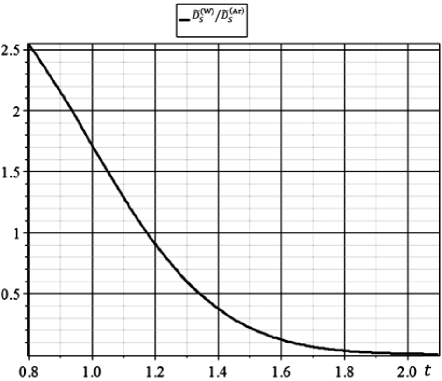
Fig. 1.: Dependence of the ratio $\tilde{\mathrm{D}}_{\mathrm{s}}^{\mathrm{(}w\mathrm{)}}/\tilde{\mathrm{D}}_{\mathrm{s}}^{\mathrm{(Ar)}}$ between the diffusion coefficients of water and argon at the corresponding temperatures

In order to confirm a conclusion about an unsatisfactory character of such notions concerning the hydrogen bond, let us consider the temperature dependences of the relative values of the self-diffusion and viscosity coefficients for water ($w$) and argon (Ar).  The temperature behaviors of the self-diffusion, $\tilde{D}_{s}^{\mathrm{(}w\mathrm{)}}/\tilde{D}_{s}^{\mathrm{(Ar)}}$, and kinematic shear viscosity, ${\tilde{\nu}}^{\mathrm{(}w\mathrm{)}}/{\tilde{\nu}^{\mathrm{(Ar)}}}$, coefficient ratios are depicted in Figs. 1 and 2, respectively (here, ${\tilde{A}}=A/A{{}_{\mathrm{tr}}}$).  Attention should be paid that the coefficients are compared at the same relative temperatures $t=T/T_{\mathrm{tr}}^{(i)}$, where $T_{\mathrm{tr}}^{(i)}$ is the corresponding triple point temperature of the liquid ($i=w$ or Ar). The states of argon and water in the interval from the triple point to the critical one and supercooled water are considered.  The values of self-diffusion and viscosity coefficients for water were taken from the NIST reference database [26], and the self-diffusion coefficients for argon were calculated, by using the molecular dynamics methods [27,​ 28] because of the lack of detailed experimental results.

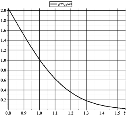
Fig. 2.: Dependence of the ratio $\tilde{\nu}_{\mathrm{s}}^{\mathrm{(}w\mathrm{)}}/\tilde{\nu}_{\mathrm{s}}^{\mathrm{(Ar)}}$ between the coefficients of kinematic shear viscosity in water and argon at the corresponding temperatures

Table 1.: Self-diffusion coefficient
of water molecules in aqueous solutions
of single-charged electrolytes [34]

			$\rm LiBr(30)$	$\rm LiI(24.8)$
$\mathrm{D}_{\mathrm{s}}^{(w)}\times 10^{5},\leavevmode\nobreak\ \text{сm${}^{2}$/s}$			2.3	2.18
		$\rm NaCl(15.9)$	$\rm NaBr(16.5)$	$\rm NaI(16.1)$
$\mathrm{D}_{\mathrm{s}}^{(w)}\times 10^{5},\leavevmode\nobreak\ \text{сm${}^{2}$/s}$		2.14	2.26	2.38
	$\rm KF(15)$	$\rm KCl(16.1)$	$\rm KBr(16.1)$	$\rm KI(16.4)$
$\mathrm{D}_{\mathrm{s}}^{(w)}\times 10^{5},\leavevmode\nobreak\ \text{сm${}^{2}$/s}$	1.99	2.44	2.68	2.8

As one can see from the dependences exhibited in Figs. 1 and 2, hydrogen bonds practically do not manifest themselves in the temperature behavior of the diffusion and viscosity coefficients. First, the self-diffusion coefficient of water exceeds that of argon, which completely agrees with a higher mobility of lighter water molecules (by order of magnitude, the self-diffusion coefficient ${\tilde{\mathrm{D}}}_{\mathrm{s}}\sim k_{\mathrm{B}}T/{\nu}$).  Second, the viscosity coefficient for water is practically by an order of magnitude smaller than that of argon, which also contradicts the initial statement that hydrogen bonds may strongly affect the viscosity of water.  Moreover, in the whole temperature intervals of the liquid state existence, the self-diffusion and viscosity coefficients of both water and argon satisfy the relation

$$\mathrm{D}_{\mathrm{s}}{\nu}\sim 1/{r}_{m},$$ (1)

where ${r}_{m}$ is the radius of the molecule, i.e., this combination is close to the corresponding constant for argon or water.  The invariance of this combination for water testifies that hydrogen bonds have no substantial relation to the problem of the water viscosity behavior.

This conclusion evidently correlates with the statement made in work [23] that the behavior of viscosity is governed by the averaged interaction potential between molecules.  The averaging is a consequence of the almost free rotation of water molecules, which would be impossible in the case of rod-like hydrogen bonds.

Moreover, we attract attention to the absence of a network formed by hydrogen bonds.  This conclusion immediately results from a careful analysis of the self-diffusion coefficients and the mobilities of ions and water molecules in diluted electrolyte solutions [29].

3 Mobility of Water
Molecules in Electrolyte Solutions

In this section, the physical nature of the mobility of water molecules in diluted aqueous solutions of electrolytes, when there are no more than 15 water molecules per ion, is discussed.  Attention is focused on the fact that the behavior of the mobility coefficients of water molecules–or, in other words, their self-diffusion coefficient–is ultimately determined by the radii of ionic hard cores.  Hence, the network of hydrogen bonds, the existence of which is postulated in the overwhelming majority of works, does not manifest itself.

3.1 Self-diffusion coefficients
of water molecules

First of all, we would like to attract attention to how the behavior of the self-diffusion coefficients of water molecules depends on the dimensions of cations and anions.  The corresponding values of self-diffusion coefficients $\mathrm{D}_{\mathrm{s}}^{(w)}$ of water molecules in several diluted electrolyte solutions at the temperature $T=296$ K are listed in Table 1.  In each of three table rows, the cation remains the same, i.e., Table 1 exhibits the dependence of $\mathrm{D}_{\mathrm{s}}^{(w)}$ on the anion size.  The solution concentration in the table is presented by the number $z_{w}$ of water molecules per ion.  The $z_{w}$-value is shown in parentheses near the chemical formula of electrolyte, e.g., NaCl(15,9).  Hence, the minimum value $z_{w}=15$ corresponds to an electrolyte concentration of 3.3 mol.%.  At such a concentration, the mutual influence of cations and anions can be neglected with a satisfactory accuracy.  Table 1 should also include the self-diffusion coefficient of water molecules in the solution CsI(17,4), namely, $\mathrm{D}_{\mathrm{s}}^{(w)}=2{.}71\times 10^{5}\leavevmode\nobreak\ \mathrm{cm}^{\mathrm{2}}\mathrm{/s}$.  In accordance with works [32,​ 33], the self-diffusion coefficient of molecules in water at the same temperature $T=296$ K equals

$$\mathrm{D}_{\mathrm{s}}^{(w)}=2{.}35\times 10^{-5}\leavevmode\nobreak\ \mathrm{cm}^{\mathrm{2}}\mathrm{/s}.$$ (2)

One can see that the self-diffusion coefficients of water molecules grow as the sizes of cations (the data in columns) and anions (the data in rows) increase, which could testify to a destruction of the hydrogen bond network. At the same time, in this case, water molecules would have freely surrounded electrolyte ions to form hydration spheres and to give rise to a substantial reduction of the self-diffusion coefficients of water molecules, which contradicts the data quoted in Table 1.

3.2 Features in the dependence
of the self-diffusion coefficients of water
molecules on the ion size

To make the analysis of the results quoted in Table 1 more comprehensive, let us consider the correlations between the self-diffusion coefficients of water molecules in electrolyte solutions and the radii of dissolved ions.  The considered radii of ions (i) were determined from crystallographic data, (ii) were selected in a way to favor the correct reconstruction of the molecular dynamics in electrolyte solutions with the use of computer simulation methods, and (iii) were evaluated from the ionic polarizability values.

The first row in Table 2 contains the values of crystallographic radius $r_{c}$ of ions [35].  The second row contains the radii of ions $r_{\sigma}$ determined in computer experiments aimed at the description of the dispersion (van der Waals) interaction between ions and water molecules [30]. The radii of ions $r_{\alpha}$, which were determined from ionic polarizabilities $\alpha$, by using the formula [36]

$$r_{\alpha}=1.5\alpha^{1/3},$$ (3)

are quoted in the third row.  The radii $r_{c}$, $r_{\sigma}$, and $r_{\alpha}$ will be referred to as hard ionic radii.

From Tables 1 and 2, it follows that the dependences of the self-diffusion coefficients of water molecules on the radii of ionic hard cores demonstrate the following regularities:

1) for diluted lithium and sodium electrolyte solutions, in which $r_{c}<\frac{1}{2}l_{w}$, where $l_{w}$ is the average distance between the oxygen atoms in neighbor water molecules, the inequality $\mathrm{D}_{\mathrm{s}}^{(w)}(\mathrm{el})<\mathrm{D}_{\mathrm{s}}^{(w)}$ is obeyed.  The inequality $r_{c}<\frac{1}{2}l_{w}$ is obviously violated only for Cs⁺.  In the solutions of potassium electrolytes, in which $r_{c}(\mathrm{K^{+}})\sim\frac{1}{2}l_{w}$, a transition from the previous inequality between the self-diffusion coefficients of water molecules to the inequality $\mathrm{D}_{\mathrm{s}}^{(w)}(\mathrm{el})>$ $>\mathrm{D}_{\mathrm{s}}^{(w)}$ is observed;

2) in electrolyte solutions with a fixed cation, but for the lithium one, the self-diffusion coefficients of water molecules grow together with the anion radius;

3) in the lithium electrolytes, the character of the dependence of $\mathrm{D}_{\mathrm{s}}^{(w)}(\mathrm{el})$ on the anion radius is opposite to that described in the previous item.

Table 2.: Hard core radii (three upper
rows) and Stokes radii of cations and anions

	$\rm Li^{+}$	$\rm Na^{+}$	$\rm K^{+}$	$\rm Cs^{+}$	$\rm F^{-}$	$\rm Cl^{-}$	$\rm Br^{-}$	$\rm I^{-}$
$r_{c}$, Å	0.6	0.95	1.33	1.69	1.36	1.81	1.95	2.16
$r_{\sigma}$, Å	0.76	1.3	1.67	1.94	1.56	2.2	2.27	2.59
$r_{\alpha}$, Å	0.45	1.12	1.41	2.02	1.51	2.33	2.55	2.93
$r_{s}^{(\mu)}$, Å	2.38	1.84	1.25	1.19	1.66	1.21	1.18	1.19
$r_{c}^{(D)}$, Å	1.91	1.88	1.14	1.15	1.77	1.33	1.22	1.35

Since the concentrations of different single-charged cations and anions are close to one another, the differences in the behavior of $\mathrm{D}_{\mathrm{s}}^{(w)}(\mathrm{el})$ can be associated with geometrical factors and their different action on the structure of local environment (hydration effects).  The former possibility should be rejected, because the geometrical obstacles should diminish with the reduction of the cation radius, which contradicts experimental data.  At the same time, a local restructuring of water in close vicinities of cations and anions turns out more appreciable for larger radii of their hard cores.

It should be noted that the effect of local restructuring in the solution is insignificant, because an increase or a reduction of the self-diffusion coefficient for water molecules in most cases does not exceed 10% and is proportional to the molar concentration of electrolyte admixtures.  All those facts are completely incompatible with the statement about the presence of a developed network of hydrogen bonds in water and diluted aqueous electrolyte solutions.

3.3 Nonideality degree of electrolyte solutions

The results obtained should be appended with the data concerning the nonideality degree of diluted electrolyte solutions, which were obtained in work [29].  According to the cited work, the nonideality degree can be calculated using the relation

$$\delta=\frac{\rho}{{\rho_{w}^{(0)}}}\left[{1+x\left(\!{\frac{{\rho_{w}^{(0)}}}{{\rho_{\mathrm{el}}^{(0)}}}-1}\!\right)}\!\right]-1,$$ (4)

where ${{\rho_{w}^{(0)}}}$ and ${\rho_{\mathrm{el}}^{(0)}}$ are the densities of water and electrolyte, respectively, in the liquid or amorphous state, and $\rho$ is the density of the aqueous electrolyte solution.  The densities of some electrolyte solutions can be found in Table 3, and the degrees of their nonideality, $\delta$, are given in Table 4.

Table 3.: Densities of aqueous electrolyte
solutions at the fixed concentration $x_{\mathrm{el}}=4\mathrm{\leavevmode\nobreak\ wt.\%}$

	$\mathrm{F}^{-}$	$\mathrm{Cl}^{-}$	$\mathrm{Br}^{-}$	$\mathrm{I}^{-}$
$\mathrm{Li}^{+}$		1.02	1.031	1.033
$\mathrm{Na}^{+}$		1.026		1.035
$\mathrm{K}^{+}$	1.032		1.029	1.032
$\mathrm{Cs}^{+}$	1.034	1.035

Table 4.: Parameters of solution
nonideality at the fixed concentration $x_{\mathrm{el}}=4\mathrm{\leavevmode\nobreak\ wt.\%}$

	$\mathrm{Cl}^{-}$	$\mathrm{Br}^{-}$	$\mathrm{I}^{-}$
$\mathrm{Li}^{+}$	$-$0.001
$\mathrm{Na}^{+}$	0.003
$\mathrm{K}^{+}$		0.003	0.004
$\mathrm{Cs}^{+}$	0.005

Note that the values of nonideality parameter obtained by formula (4) are averaged over the number of water molecules that surround the corresponding ion.  One can see that relatively small values of the mobility of lithium cations and the self-diffusion coefficient of water molecules in the lithium electrolytes correspond to negative nonideality degrees.  This fact testifies that lithium cations do not promote the formation of hydration spheres around them with the density exceeding that of water.  In other cases, if one may talk about the formation of hydration spheres, the smallness of the parameter $\delta$ testifies that their influence on the density in diluted electrolyte solutions is weak.

From the facts mentioned above, it follows that

(i) the key role in governing the transport properties of aqueous electrolyte solutions–first of all, the behavior of the mobility coefficients of ions and water molecules–is played by hard cores of those objects;

(ii) the conventional scenario that ions in aqueous solutions move through “voids” existing in the hydrogen bond network is incorrect;

(iii) hydrogen bonds between water molecules have to be considered as a convenient model, which to a certain extent reflects the existence of correlations between the dipole moments of molecules, as well as multipole moments of higher orders; and

(iv) the role of hydration effects is insignificant and can be taken into account in the framework of the thermodynamic perturbation theory.

4 Experimental Evidence
for the Similarity of the Thermodynamic
Properties of Water and Argon

In this section, some facts testifying to the thermodynamic similarity between water and argon and, hence, calling into question the conventional viewpoint about the crucial role of hydrogen bonds in the formation of water properties are presented.  With that end in view, let us consider the temperature dependences for the simplest quantities: the fractional volume (this is one of the mechanical characteristics of the system) and the evaporation heat (the most important among the thermal parameters).  In parallel, the behavior of ordinary water and its heavy counterpart, which considerably differ from each other by the character of molecular rotational motion, will be analyzed.

The temperature dependences of the fractional volumes $\upsilon^{(i)}$ of water ($i=w$) and argon ($i=\mathrm{Ar}$) at their coexistence curves will be compared in the spirit of the similarity principle for the corresponding states of the system [31].  This means that the ratio ${R_{\upsilon}^{(\mathrm{H}_{2}\mathrm{O})}(t)=\tilde{\upsilon}^{(\mathrm{H}_{2}\mathrm{O})}(t)/\tilde{\upsilon}^{(\mathrm{Ar})}(t)}$ between the normalized volumes ${\tilde{\upsilon}^{(i)}(t)=\upsilon^{(i)}(t)/\upsilon_{c}^{(i)}}$, where ${\upsilon_{c}^{(i)}}$ means the $\upsilon^{(i)}(t)$-value at the corresponding critical point, should be considered as a function of the dimensionless temperature $t=T/T_{c}^{(i)}$, where $t=T/T_{c}^{(i)}$ is the critical temperature of the $i$-th liquid.  As is seen from Fig. 3, practically in the whole temperature interval of water existence in the liquid state, $0.42<t<0.9$, the temperature dependences of the fractional volumes of water and argon are similar.  Their ratio $R_{\upsilon}^{(\mathrm{H}_{2}\mathrm{O})}(t)$ in the temperature interval $0.55<t<0.8$ is approximated with a satisfactory accuracy by the linear dependence

$$R_{\upsilon}^{(\mathrm{H}_{2}\mathrm{O})}(t)=r_{0}^{(\upsilon)}+4r_{\mathrm{H}}^{(\upsilon)}(1-\lambda_{\upsilon}\,t)$$ (5)

with the coefficients

$$\begin{array}[]{l}\displaystyle\mathrm{H}_{2}\mathrm{O}:r_{0}^{(\upsilon)}=0.827\leavevmode\nobreak\ r_{\mathrm{H}}^{(\upsilon)}=0.021\leavevmode\nobreak\ \lambda_{\upsilon}=0.83,\\[8.53581pt] \displaystyle\mathrm{D}_{2}\mathrm{O}:r_{0}^{(\upsilon)}=0.851\leavevmode\nobreak\ r_{\mathrm{H}}^{(\upsilon)}=0.021\leavevmode\nobreak\ \lambda_{\upsilon}=0.83,\end{array}$$ (6)

i.e.  it remains almost constant.

The deviations of the ratio $R_{\upsilon}(t)=\upsilon^{(\mathrm{D}_{2}\mathrm{O})}(t)/$ $/\upsilon^{(\mathrm{H}_{2}\mathrm{O})}(t)$ from unity is appreciable only for at $t\ll$ $\ll 0.55$ and in a vicinity of the critical point. However, they do not exceed 4%.

A comparison between the evaporation heats for water and argon is even more intriguing (see Fig. 4).  The deviation of $R_{q}^{(\mathrm{H}_{2}\mathrm{O})}(t)$ from an approximate value of about 6.2 does not exceed 1.1%.

Analogously to formula (5), the ratio $R_{q}^{(\mathrm{H}_{2}\mathrm{O})}(t)$ in the temperature interval $0.55<t<0.8$ is quasilinear,

$$R_{q}^{(\mathrm{H}_{2}\mathrm{O})}(t)=r_{0}^{(q)}+4r_{\mathrm{H}}^{(q)}(1-\lambda_{q}\,t),$$ (7)

where

$$\begin{array}[]{l}\displaystyle\mathrm{H}_{2}\mathrm{O}:r_{0}^{(q)}=6.137\leavevmode\nobreak\ \leavevmode\nobreak\ r_{\mathrm{H}}^{(q)}=0.080\leavevmode\nobreak\ \lambda_{q}=0.85\\[8.53581pt] \displaystyle\mathrm{D}_{2}\mathrm{O}:r_{0}^{(q)}=6.084\leavevmode\nobreak\ r_{\mathrm{H}}^{(q)}=0.182\leavevmode\nobreak\ \leavevmode\nobreak\ \lambda_{q}=0.85.\end{array}$$ (8)

Moreover, the linear functions $1-\lambda_{\upsilon}t$ and $1-\lambda_{q}t$ in Eqs. (5) and (7), respectively, are almost identical, which testifies to their common origin.  In works [17,​ 23], it was shown that those functions are generated by weak hydrogen bonds.

Small deviations of ${R_{\upsilon}^{(i)}(t)}$ and ${R_{q}^{(i)}(t)}$ from their constant values evidently testify to a weak effect of hydrogen bonds and a similarity of intermolecular potentials in water and argon.  The latter conclusion has a completely natural explanation.  The behavior of the fractional volume and the evaporation heat for water is governed by the averaged potential of interaction between molecules.  In its turn, the potential averaging is a direct consequence of the rotational motion of water molecules.  As a result, the anisotropic effects associated with weak hydrogen bonds become practically smoothed out.

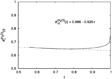
Fig. 3.: Temperature dependences of the ratio $R_{\upsilon}^{(\mathrm{H}_{2}\mathrm{O})}(t)=$ $=\tilde{\upsilon}^{(\mathrm{H}_{2}\mathrm{O})}(t)/\tilde{\upsilon}^{(\mathrm{Ar})}(t)$ calculated at the coexistence curves of water and argon in accordance with experimental data [26]

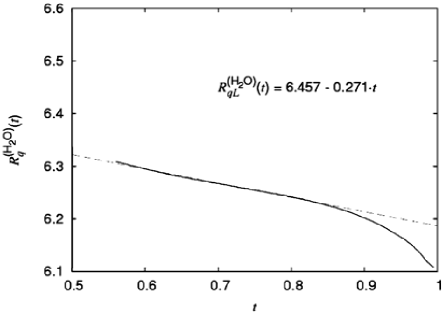
Fig. 4.: Temperature dependences of the ratio $R_{q}^{(\mathrm{H}_{2}\mathrm{O})}(t)=$ $=q^{(\mathrm{H}_{2}\mathrm{O})}(t)/q^{(\mathrm{Ar})}(t)$ in accordance with experimental data [26]

5 Vibration Frequencies
of Hydrogen Atoms in the Water Molecule
in Vapor, Water, and Ice

Let us discuss the frequency shift for the longitudinal (valence) vibrations of the hydrogen ion H${}_{1}^{+}$ in a water molecule, which lies close to the line connecting the centers of mass of oxygen atoms in two neighbor water molecules composing a dimer (see Fig. 5).  The corresponding vibration frequencies are determined by the formula

$$\omega_{\parallel}\approx\sqrt{\frac{{{\rm K}_{{\rm{rr}}}^{{\rm(1)}}}}{{{\rm M}_{{\rm Re}}}}},$$ (9)

where the force constant (the dimensionless quantities $\tilde{\Phi}=\Phi/k_{\mathrm{B}}T_{\mathrm{tr}}$ and $\tilde{r}_{{{{\mathrm{H}}}}_{k}}=r_{{{{\mathrm{H}}}}_{k}}/\sigma$, where $\sigma=298$ Å is the oxygen diameter, will be used) is defined in a standard way:

$${\tilde{\rm K}_{\rm{rr}}^{{\rm(1)}}=\frac{{\partial^{\rm 2}{\rm\tilde{\Phi}}_{\rm 2}^{{\rm(1)}}}}{{\partial{\rm\tilde{r}}_{{\rm H}_{\rm 1}}^{\rm 2}}}}|_{{\rm\tilde{r}^{\prime}}_{{\rm H}_{\rm 1}}},$$ (10)

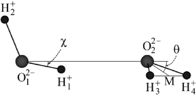
Fig. 5.: Configuration of a linear dimer of water molecules. The equilibrium angle values are $\chi=3.76^{\circ}$ and $\theta=41.1^{\circ}$

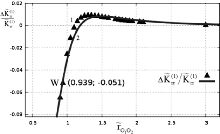
Fig. 6.: Dependences of the relative change $\Delta\tilde{\mathrm{K}}_{\mathrm{rr}}^{{(1)}}/\tilde{\mathrm{K}}_{\mathrm{rr}}^{{(1)}}$ of the force constant on the distance $\tilde{r}_{{{\mathrm{O}}_{\mathrm{1}}{\mathrm{O}}_{\mathrm{2}}}}$ in the standard dimer: with regard for a mutual tuning of molecular orientations (1, triangles) and for the fixed orientation of molecules as in the configuration in Fig. 5 (2, curve)

Table 5.: Force constants for water molecules

	$\frac{{\partial^{2}\tilde{\Phi}}}{{\partial\tilde{r}_{1}^{2}}}$	$\frac{{\partial^{2}\tilde{\Phi}}}{{\partial\theta^{2}}}$	$\frac{{\partial^{2}\tilde{\Phi}}}{{\partial\tilde{r}_{1}\partial\theta}}$
GSD	256.98	182.15	33.439
Experim. [9]	256.98	190.64	33.439

and the reduced mass of the oxygen–hydrogen system in the water molecule approximately equals

$${\rm M}_{{\rm Re}}\approx\frac{{\left({{\rm M}_{\rm O}+{\rm M}_{\rm H}}\right){\rm M}_{\rm H}}}{{\left({{\rm M}_{\rm O}+{\rm M}_{\rm H}}\right)+{\rm M}_{\rm H}}}.$$ (11)

The approximate character of Eq. (11) is explained by the fact that hydrogen H${}_{2}^{+}$ (see Fig. 5) is not located at the line connecting the centers of mass of oxygen atoms.  The double derivative in Eq. (10) is assumed to be taken at the point $\tilde{r}_{\mathrm{H}_{\mathrm{1}}}^{\prime}$ determined by the equation

$${\frac{{\partial\left({\tilde{\Phi}_{{{\mathrm{1}}}}^{{{\mathrm{(1)}}}}({\widetilde{\mathrm{\bf{r}}}}_{{{{\mathrm{H}}}}_{{{\mathrm{1}}}}},{\widetilde{\mathrm{\bf{r}}}}_{{{{\mathrm{H}}}}_{{{\mathrm{2}}}}})\!+\!\tilde{\Phi}_{{{\mathrm{Int}}}}({\bf\tilde{r}}_{{{\rm O}_{\rm 1}{\rm H}_{\rm 3}}},{\bf\tilde{r}}_{{{\rm O}_{\rm 1}{\rm H}_{\rm 4}}},{\bf\tilde{r}}_{{{\mathrm{O}}_{\mathrm{1}}{\mathrm{O}}_{\mathrm{2}}}})}\right)}}{{\partial{\rm\tilde{r}}_{{{\rm H}_{\rm 1}}}}}}\biggl{|}_{{\rm\tilde{r}^{\prime}}_{{{\rm H}_{\rm 1}}}}\!\!=0.$$ (12)

It should be noted that Eq. (12) gives rise to only an insignificant displacement $\Delta\mathrm{\tilde{r}}_{{\mathrm{H}_{\mathrm{1}}}}$ of the equilibrium position of hydrogen H${}_{1}^{+}$.  Assuming that

$${\rm\tilde{r}}_{{\mathrm{H}_{\mathrm{1}}}}^{\prime}={\rm\tilde{r}}_{{\mathrm{H}_{\mathrm{1}}}}+\Delta{\rm\tilde{r}}_{{\mathrm{H}_{\mathrm{1}}}},$$

where

$$|\Delta{\rm\tilde{r}}_{{\mathrm{H}_{\mathrm{1}}}}|\ll{\rm\tilde{r}}_{{\mathrm{H}_{\mathrm{1}}}},$$

the value of $\Delta{\rm\tilde{r}}_{{\mathrm{H}_{\mathrm{1}}}}$ can be determined with the help of a more simple equation,

$${\widetilde{\mathrm{K}}_{{\mathrm{rr}}}^{{\mathrm{(1)}}}\Delta{\rm\tilde{r}}_{{\rm H}_{\rm 1}}+\vec{\nabla}_{{\rm\tilde{r}}_{{\rm H}_{\rm 1}}}\widetilde{\Phi}_{{\rm{Int}}}({\tilde{\rm{\bf r}}}_{{\rm O}_{\rm 1}{\rm H}_{\rm 3}},{\tilde{\rm{\bf r}}}_{\scriptscriptstyle{\rm O}_{\rm 1}{\rm H}_{\rm 4}},{\tilde{\rm{\bf r}}}_{{\rm O}_{\rm 1}{\rm O}_{\rm 2}})}\biggl{|}_{{\rm\tilde{r}}_{{{\mathrm{H}}_{\mathrm{1}}}}={\rm\tilde{r}^{\prime}}_{{\rm H}_{\rm 1}}}\!\!=0,$$ (13)

where ${\tilde{\mathrm{K}}}_{\mathrm{rr}}^{{\mathrm{(1)}}}$ is the elasticity coefficient for the bond between the hydrogen and oxygen atoms in the monomer.

One may get convinced (see work [25]) that, by the order of magnitude in the framework of the electrostatic model, the ratio $\Delta{\rm\tilde{r}}_{{\mathrm{H}_{\mathrm{1}}}}/{\rm\tilde{r}}_{{\mathrm{H}_{\mathrm{1}}}}$, where $\Delta{\rm\tilde{r}}_{{\mathrm{H}_{\mathrm{1}}}}=$ $={\rm\tilde{r}}_{{\mathrm{H}_{\mathrm{1}}}}^{\prime}-{\rm\tilde{r}}_{{\mathrm{H}_{\mathrm{1}}}}$, satisfies the inequality

$$\Delta{\rm\tilde{r}}_{{{\rm H}_{\rm 1}}}/{\rm\tilde{r}}_{{{\rm H}_{\rm 1}}}\sim({{\rm\tilde{r}}_{{{\rm H}_{\rm 1}}}/{{\rm\tilde{r}}_{{{\mathrm{O}}_{\mathrm{1}}{\mathrm{O}}_{\mathrm{2}}}}}})^{4}\leq 0.02.$$

Therefore, the displacement of a hydrogen atom can be neglected practically for all distances between the oxygen atoms in the water dimer.

The values of force constants for the water molecule, which correspond to the GSD potential, are listed in Table 5.  For the sake of comparison, Table 5 also contains the corresponding force constants determined experimentally.

The force constant for symmetric valence vibrations in the equilibrium configuration of a dimer shown in Fig. 5 can be calculated by formula (10). The dependence of the relative change of a force constant on the distance between the oxygens in the dimer is depicted in Fig. 6.  Point W with the coordinates $(0.939,-0.051)$ corresponds to the distance $r{{}_{{{\mathrm{O}}_{\mathrm{1}}{\mathrm{O}}_{\mathrm{2}}}}}=2{.}8$ Å between the oxygen atoms, which is typical of water near its triple point.  The relative change of the constant of symmetric valence vibrations at this point equals $\Delta\tilde{\mathrm{K}}_{\mathrm{rr}}^{{(1)}}/\tilde{\mathrm{K}}_{\mathrm{rr}}^{{(1)}}=-0.05$. Hence, the values of the force constant of valence vibrations at the distances between the oxygen atoms corresponding to a dimer at equilibrium and to liquid water differ from each other by 5%.

5.1 Results of calculations
of the valence vibration frequencies
for hydrogen atoms in the water molecule

The frequency shift of hydrogen valence vibrations in the water molecule depends on the water phase state and can reach several hundreds of inverse centimeters (Table 6).  In this work, we assume that the main contribution to the experimentally observed frequency shift is made by electrostatic forces associated with multipole moments of water molecules.

The major result of our research consists in that the electrostatic forces really induce the frequency shifts, which agree with experimental data by both the shift direction and the order of magnitude.  The frequency shift of valence vibrations equals

$${\rm\Delta\omega}\approx\frac{{\rm 1}}{{\rm 2}}{\rm\omega}_{\rm 0}\frac{{\Delta\widetilde{\rm K}_{\rm{rr}}^{{(1)}}}}{{\widetilde{\rm K}_{\rm{rr}}^{{(1)}}}},$$

where $\omega_{0}\approx 3657\leavevmode\nobreak\$cm^-1 is the vibration frequency for an isolated water molecule.  The relative increase of the elastic constant $\Delta\tilde{\mathrm{K}}_{\mathrm{rr}}^{{(1)}}/\tilde{\mathrm{K}}_{\mathrm{rr}}^{{(1)}}$ at $r_{{{\mathrm{O}}_{\mathrm{1}}{\mathrm{O}}_{\mathrm{2}}}}=2.8$ Å amounts to $-0.05$, i.e.  $\Delta\omega\approx-91.43$ cm^-1. Hence, the frequency shift sign for a dimer correlates with those in liquid water and ice.  The shear moduli are identical by order of magnitude, but, nevertheless, they are considerably different.  This fact has a simple qualitative interpretation.  The total electric field that acts on a water molecule in the liquid is, on the average, a little larger than that acting from the neighbor molecule in the dimer.  An insignificant increase of the electric field strength in the liquid is connected with a weakly ordered arrangement of the centers of mass of molecules and the orientations of its nearest neighbors.  As a consequence, owing to the superposition principle, only a weak strengthening of the electric field in the molecule occurs.  The opposite situation takes place in ice.

Let us discuss the change of elastic constant in the standard dimers (see Fig. 5) at $r_{{{\mathrm{O}}_{\mathrm{1}}{\mathrm{O}}_{\mathrm{2}}}}=2.85$ Å.  This is a distance between the oxygen atoms of water molecules in an argon matrix.  According to our calculations, the relative increase of the elastic constant $\Delta\tilde{\mathrm{K}}_{\mathrm{rr}}^{{(1)}}/\tilde{\mathrm{K}}_{\mathrm{rr}}^{{(1)}}$ for this dimer configuration amounts to $-0.0443$ for the fixed orientation of molecules as in the standard dimer and to $-0.0432$ if the orientations of molecules can be adjusted.  These variations of the elastic constant correspond to a valence vibration frequency of 3576 cm^-1 in the former case and 3578 cm^-1 in the latter one.  It should be noted that the relatively small value of orientational contribution is explained by the fact that the parameter of the system $r_{{{\mathrm{O}}_{\mathrm{1}}{\mathrm{O}}_{\mathrm{2}}}}=2.85$ Å is in the interval, where the dependence of the repulsion energy between molecules monotonically decreases.  The frequency obtained from experiments in the argon matrix [38] equals 3574 cm^-1.  Therefore, we believe that it is possible to talk about a complete coincidence of calculated and experimental results.  From our viewpoint, this is a powerful argument in favor that the frequency shift of valence vibrations has the electrostatic origin.

Table 6.: Frequencies of symmetric
valence vibrations of hydrogen atoms
in the water molecule in vapor, water, and ice

	$\nu_{\rm v},\leavevmode\nobreak\ \text{сm}^{-1}$	$\nu_{\rm w},\leavevmode\nobreak\ \text{сm}^{-1}$	$\nu_{\rm{Ice}},\leavevmode\nobreak\ \text{сm}^{-1}$
Experim. [15]	3657	3490	3200
Experim. [37]	3656.7	3280
MST-FP [37]	3656	3251
SPC-FP [37]		3875

It is very important that the explanation of the frequency shifts different by magnitude is principally based on the superposition principle, the application of which to sharply directed and saturated irreducible hydrogen bonds is impossible.  In order to make the substantiation of this fact more complete, we intend to consider the frequency shifts of valence vibrations in ice and liquid water elsewhere.

Not less demonstrative is the circumstance that one should expect a positive sign of the frequency shift in rarefied vapor, which directly follows from the behavior of $\Delta\tilde{\mathrm{K}}_{\mathrm{rr}}^{{(1)}}/\tilde{\mathrm{K}}_{\mathrm{rr}}^{{(1)}}$ in Fig. 6.  This fact is also supported qualitatively by the experimental data on IR absorption in rather rarefied water vapor [39].

6 Influence of Neighbor Molecules
on the Dipole Moment of a Water Molecule

The dipole moment of an isolated water molecule is determined as a sum of two oppositely directed vectors of dipole moments, $\bm{\mu}={\bm{\mu}}_{\mathrm{H}}+{\bm{\mu}}_{\mathrm{O}}$.  The dipole moment ${\bm{\mu}}_{\mathrm{H}}$ is determined by the spatial distribution of the centers of oxygen’s negative charge and hydrogens’ positive charges, ${\bm{\mu}}_{\mathrm{H}}=q_{\mathrm{H}}(\mathbf{r}_{1}+\mathbf{r}_{2})$.  The absolute value of dipole moment ${\bm{\mu}}_{\mathrm{H}}$ equals $\mu_{\mathrm{H}}=$ $=2q_{\mathrm{H}}r_{\mathrm{OH}}\cos\left(\theta/2\right)=5{.}6281$ D.  The dipole momentum of the oxygen atom ${\bm{\mu}}_{\mathrm{O}}$ emerges owing to the polarization of the oxygen anion’s electron shell in the electric field created by hydrogen atoms in the water molecule.  According to work [9], it equals

$${\bm{\mu}}_{\rm O}=-\alpha q_{\rm H}\left(\!{\frac{{{\bf{r}}_{1}}}{{r_{1}^{3}}}\left[{1-K(r_{1})}\right]+\frac{{{\bf{r}}_{2}}}{{r_{2}^{3}}}\left[{1-K(r_{2})}\right]}\!\right)\!.$$

It is easy to make sure that $\mu_{\mathrm{O}}=-3.7752$ D.  Together with ${\bm{\mu}}_{\mathrm{H}}$, the following value is obtained for the absolute value of dipole moment $\bm{\mu}$: $\mu=\mu_{\mathrm{H}}+\mu_{\mathrm{O}}=$ $=1.8528$ D.  It completely agrees with the absolute value of dipole moment in an isolated water molecule.

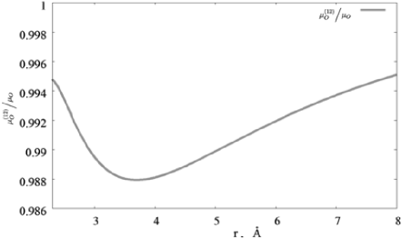
Fig. 7.: Dependence of the ratio $\mu_{\mathrm{O}}^{(12)}/\mu_{\mathrm{O}}$ on the distance between oxygen atoms in two water molecules

The variation of the dipole moment under the action of a neighbor molecule is one of the simplest manifestations of many-particle effects in the system.  To estimate the influence of the second molecule, let us calculate the ratio $\mu_{\mathrm{O}}^{(12)}/\mu_{\mathrm{O}}$ between the dipole moments of the oxygen atom in the pair approximation ($\mu_{\mathrm{O}}^{(12)}$, see work [3]) and in the isolated water molecule ($\mu_{\mathrm{O}}$).  The calculated dependence of $\mu_{\mathrm{O}}^{(12)}/\mu_{\mathrm{O}}$ on the distance between the oxygen atoms in two neighbor molecules is depicted in Fig. 7.

One can see from Fig. 7 that the variation of the dipole moment of the oxygen atom under the influence of the electric field created by the neighbor molecule does not exceed 1.5%.  The same can also be said about the component ${\bm{\mu}}_{\mathrm{H}}$.  From whence, it follows that the effects of electron shell overlapping, which are responsible for the change of the dipole moment of a water molecule, are insignificant.  This result completely agrees with the conclusions of works [4,​ 5,​ 6,​ 7].  Consequently, this means that the irreducible components of the interaction between molecules, which have to be regarded as hydrogen bonds, are much smaller in comparison with the energy of electrostatic interaction between molecules.

7 Arguments in Favor
of the Existence of a Hydrogen Bond

In the previous sections, we presented the facts, whose explanation does not need the hypothesis about the existence of hydrogen bonds in water and other classical liquids according to L.A. Bulavin’s classification [18].  However, in this section, we describe a phenomenon, which cannot be explained without attracting the hydrogen bond concept.  This is the temperature dependence of the water heat capacity.  For convenience, this parameter will be reckoned in the dimensionless units $i_{Q}={2C_{V}}/\left(k_{\mathrm{B}}N_{\mathrm{A}}\right)$, where ${C_{V}}$ is the heat capacity of a gram molecule, and $N_{\mathrm{A}}$ Avogadro’s constant.  These dimensionless units for the heat capacity will be called the number of thermal degrees of freedom.

The latter differs from the standard number of degrees of freedom in that the number of vibrational degrees of freedom in it doubles.  Argon can serve as the simplest example here.  In rarefied vapor, an argon atom is described by three independent coordinates, which give its spatial position.  The corresponding value of $i_{Q}$ also equals 3.  In the crystalline state of argon, the number of standard degrees of freedom for its atoms also equals 3.  However, $i_{Q}=6$, because each degree of freedom corresponds to the vibrational motion.

The number $i_{Q}$ of thermal degrees of freedom per water molecule consists of three components,

$$i_{Q}=i_{Q}^{(\mathrm{tr})}+i_{Q}^{(\mathrm{or})}+i_{Q}^{(\upsilon)},$$

which correspond to the translational motion of the molecules, their rotation, and probable vibrations of irreducible hydrogen bonds, which are formed in all water phases [40,​ 41].

From Fig. 8, one can see that the maximum value of heat capacity equals 6 for Ar in the liquid phase, 12 for hydrogen sulfide, and reaches 20 and even more for water.  The maximum value corresponds to a situation where every of the ordinary degrees of freedom has a vibrational character.

The heat capacity of liquid argon turns out some lower than in the solid state; nevertheless, it is close to 6.  In the case of hydrogen sulfide, three orientational degrees of freedom have also to be taken into account.  If they have been vibrational, the maximum $i_{Q}$-value would have been close to 12.  Water would also have had this value for the number of thermal degrees of freedom per molecule if its molecules have not been bound with one another by means of hydrogen bonds.  However, actually, as one can see, the number $i_{Q}$ for water exceeds this value approximately by 6.

From the physical viewpoint, this difference has a natural explanation: there are weak hydrogen bonds between molecules, which practically do not interfere with the rotational motion of the molecules, but make additional contributions to the water heat capacity.  These contributions result from two transverse and one longitudinal vibrations of the hydrogen bond.  Since every vibration corresponds to two thermal degrees of freedom, the excitation of all vibrations for only one hydrogen bond results in the heat capacity growth by 6.

A more detailed analysis of the problem shows [17] that, in order to attain a complete agreement with experimental data, it suffices to admit that every molecule of liquid water forms 2.5 hydrogen bonds near the triple point temperature and only one hydrogen bond in a vicinity of the critical point. Those estimations are in quite satisfactory agreement with the results of works [42,​ 43], as well as with the results of computer calculations.

8 Hydrogen Bond
from the Viewpoint
of the Chemical Bond Theory

The hydrogen bond concept seems to appear for the first time in the work by A.R. Hantzsch in 1909 [44].  Using the water molecule as an example, the sense of this new concept can be interpreted in the following way.  The hydrogen bond is a new type of interaction between two water molecules.  It acts along the O–H–O line and is associated with the emergence of a specific interaction between the indicated groups of molecules that arises at certain distances between them.  The introduced interaction is much stronger than the van der Waals one, but, at the same time, is much weaker than the covalent bond and the ionic interaction.  In work [45], an attempt was made to identify this specific interaction with the covalent bond between the hydrogen atom, which can hold two electron pairs about itself, and two electronegative atoms.  L. Pauling criticized this approach [46] and presented arguments in favor of the ionic nature of a hydrogen bond. Supposing that the hydrogen bond has a sharply directed character and is saturated, i.e.  it does not agree with the superposition principle, L. Pauling calculated the residual entropy of ice ($=k_{\mathrm{B}}\ln(3/2)$) and showed that this value agrees well with experimental data (see also work [47]).  This result promoted the further propagation of the hydrogen bond concept while describing the properties of ice, water, alcohols, and so forth.

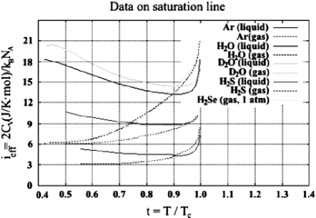
Fig. 8.: Temperature dependences of $i_{\mathrm{eff}}$ for $\mathrm{H}_{\mathrm{2}}\mathrm{O}$, $\mathrm{D}_{\mathrm{2}}\mathrm{O}$, $\mathrm{H}_{\mathrm{2}}\mathrm{S}$, and argon systems in the liquid and vapor states at the curves of their coexistence. Experimental data are taken from work [26]

9 Discussion of the Results Obtained

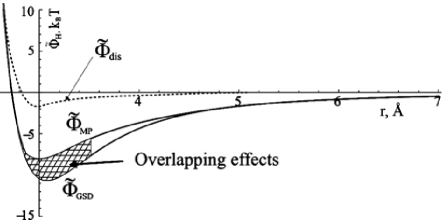
Fig. 9.: Partial contributions to the interaction potential between water molecules in the linear dimer

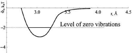
Fig. 10.: Hydrogen bond potential in the linear dimer of water molecules

Let us summarize the results presented above, being based on the general ideas concerning the structure of intermolecular potentials in classical systems.  We proceed from the fact that the simplest structure of the interaction between molecules is inherent to atomic systems of the argon type.  The corresponding potential of the intermolecular interaction $\Phi(r)$ is a sum of an attractive component $\Phi_{\mathrm{dis}}(r)$, which is associated with dispersion forces, and a component $\Phi_{\mathrm{rep}}(r)$ describing the repulsion:

$$\Phi(r)=\Phi_{\mathrm{dis}}(r)+\Phi_{\mathrm{rep}}(r).$$ (14)

Note that the known Lennard-Jones potential has just this structure.

The systems consisting of molecules like N₂ are characterized by the loss of spherical symmetry, which is accompanied by the appearance of the appreciable angular dependence in the particle-to-particle potential [48]:

$$\Phi(r)\rightarrow\Phi(r,\Omega)=\Phi_{\mathrm{dis}}(r,\Omega)+\Phi_{\mathrm{rep}}(r,\Omega).$$ (15)

This structure must also be inherent to the interaction potentials between water and alcohol molecules if the distance between them considerably exceeds the sum of their molecular radii.

However, as the molecules get closer, their electron shells overlap, and a qualitatively new component of the intermolecular interaction, $\Phi_{\mathrm{H}}(r,\Omega)$, appears, which is conventionally called the hydrogen bond energy.  In this case,

$$\Phi(r,\Omega)=\Phi_{\mathrm{dis}}(r,\Omega)+\Phi_{\mathrm{rep}}(r,\Omega)\,+$$

$$+\,\Phi_{E}(r,\Omega)+\Phi_{\mathrm{H}}(r,\Omega).$$ (16)

At the same time, the hydrogen bond energy, as a rule (see work [49]), is associated with the sum of two last terms,

$$E_{\mathrm{H}}(r,\Omega)=\Phi_{E}(r,\Omega)+\Phi_{\mathrm{H}}(r,\Omega),$$ (17)

and M.D. Sokolov was the first who attracted attention to this fact for the first time [1].

In order to estimate the irreducible contribution to the hydrogen bond energy, the following approach was proposed in work [49].  From the conventional viewpoint, the ground state energy of a water dimer is determined by the “hydrogen bond” energy $E_{\mathrm{H}}(r_{d},\Omega_{d})$, where the subscript $d$ indicates that the distance between the oxygen atoms of two water molecules and the angle values correspond to the dimer configuration.  On the other hand, the properties of dimers are described quite well, by using phenomenological intermolecular potentials of the SPC [50], SPC/E [51], TIPS [11], SD [9], GSD [3], and so forth types.

The dimer configuration is determined from the condition of interaction energy minimum.  Proceeding from this fact and expression (16), the energy of an irreducible hydrogen bond can be estimated with the help of the relation

$$\Phi_{\mathrm{H}}(r,\Omega)=\Phi(r,\Omega)\,-$$

$$-\,\left[{\Phi_{\mathrm{dis}}(r,\Omega)+\Phi_{\mathrm{rep}}(r,\Omega)+\Phi_{M}(r,\Omega)}\right]\!,$$ (18)

where $\Phi_{M}(r,\Omega)$ is the multipole approximation to the electrostatic interaction energy.  The multipole moments of a water molecule are assumed to be determined independently of effective charges governing the behavior of the phenomenological potential $\Phi(r,\Omega)$.  The magnitudes of effective charges, as well as some other parameters of phenomenological potentials, are determined by fitting the model to dimer parameters, which are determined experimentally or within quantum-chemical methods.  Hence, it is the difference on the right-hand side of Eq. (18) that describes the component emerging owing to the overlapping of electron shells in water molecules.  In work [49], the intermolecular potential $\Phi(r,\Omega)$ was simulated by the generalized Stillinger–David potential $\Phi_{\mathrm{GSD}}(r)$, so that

$$\Phi_{\mathrm{H}}(r,\Omega)=\Phi_{\mathrm{GSD}}(r,\Omega)\,-$$

$$-\left[{\Phi_{\mathrm{rep}}(r,\Omega)+\Phi_{\mathrm{dis}}(r,\Omega)+\Phi_{M}(r,\Omega)}\right]\!.$$ (19)

The general behavior of the potentials $\Phi_{\mathrm{GSD}}(r,\Omega)$, $\Phi_{M}(r,\Omega)$, and $\Phi_{\mathrm{dis}}(r,\Omega)$ for the molecular orientation typical of the dimer are exhibited in Fig. 9.

The hydrogen bond potential for the same configuration of water molecules is shown in Fig. 10.  This is a short-range potential that emerges owing to the overlapping of electron shells and has a quantum-mechanical origin.  It is this potential that should be interpreted as the hydrogen bond potential in water.  Its depth, by order of magnitude, is identical to the depth of the dispersion force interaction potential between water molecules, but it is substantially smaller by magnitude than the multipole interaction potential.  As a result, the contribution made by hydrogen bonds to the thermodynamic potentials of water can be taken into account in the framework of the thermodynamic perturbation theory.  At the qualitative level, this circumstance completely agrees with the similarity of the thermodynamic functions of water and argon at their coexistence curves.

The presented estimations of the magnitudes of the electrostatic interaction and hydrogen bond contributions to the energy of intermolecular interaction were confirmed many times in works [3,​ 4,​ 5,​ 6,​ 7].  In particular, it was shown in work [5] that, by order of magnitude,

$$\frac{\left|U_{E}(q_{1},q_{2})\right|}{\left|U_{\mathrm{H}}(q_{1},q_{2})\right|}\thicksim\frac{10}{2}.$$

This means that the influence of exactly hydrogen bonds is taken into account in a natural way by the thermodynamic perturbation theory [17,​ 23].

While analyzing the thermodynamic properties of liquids and solutions with the use of statistical theory, it is necessary to take into consideration the fact that molecules permanently rotate and, at the same time, hinder their rotational motion.  The characteristic period of the thermal rotational motion of molecules turns out much shorter than the characteristic time of changing the configurations formed by the translational degrees of freedom. Therefore, the thermodynamic properties of liquids are mainly governed by the potentials $U_{A}(r_{12})$ averaged over all angular variables (here, $r_{12}$ is the distance between the centers of mass of molecules).  In works [17,​ 23], it was demonstrated that such an averaged potential has a structure of the Sutherland potential,

$$U_{A}(r_{12})\Rightarrow\left\{\!\!{\begin{array}[c]{ll}{\infty,}&{r_{12}<r_{0}}\\ {U_{a}(r_{12}),}&{r_{12}>r_{0}},\end{array}}\right.$$ (20)

where $U_{a}(r)$ is the attraction potential, which decreases at large enough distances following the law $1/r_{12}^{6}$.  With the same accuracy, the averaged potential can be approximated by the Lennard-Jones potential [17,​ 23]:

$$\begin{array}[]{l}\displaystyle{U_{A}(r_{12})\Rightarrow U_{\rm LJ}(r_{12}),}\\[2.84526pt] \displaystyle{U_{\rm LJ}(r_{12})=-4\varepsilon\bigg{[}{\bigg{(}\!{\frac{\sigma}{{r_{12}}}}\!\bigg{)}^{\!\!12}-\bigg{(}\!{\frac{\sigma}{{r_{12}}}}\!\bigg{)}^{\!\!6}}\bigg{]}}\!.\end{array}$$ (21)

The thermodynamic properties of liquids consisting of anisotropic molecules, owing to the rotational motion of those molecules, are similar to the corresponding properties of atomic liquids of the argon type [17,​ 23].  Small differences between those properties stem from weak angular correlations, which can be taken into account with the help of perturbation theory.  The most noticeable angular correlations are observed in the temperature interval of the supercooled liquid state and at the formation of an instant local structure in liquids.  This circumstance is a precondition for the emergence of special points in aqueous alcohol solutions.

From the qualitative viewpoint, such a change of priorities is not justified, because the analytic continuation of the components $\Phi_{\mathrm{dis}}(r,\Omega)$ and $\Phi_{M}(r,\Omega)$ into the region, where electron shells overlap is not accompanied by the appearance of effects that would violate the requirement of continuity in the potential behavior.  For this reason, it is desirable that the hydrogen bond potential should be defined in another way.  According to the continuity requirement, the hydrogen bond potential will be defined, by using the formula

$$\Phi(r,\Omega)=\Phi_{\mathrm{dis}}(r,\Omega)\,+$$

$$+\Phi_{r}(r,\Omega)+\Phi_{M}(r,\Omega)+\Phi_{\mathrm{H}}(r,\Omega).$$ (22)

In the region where the electron shells overlap, the functions $\Phi_{\mathrm{dis}}(r,\Omega)$ and $\Phi_{M}(r,\Omega)$ should be substituted by their corresponding continuations from the region, where their application does not invoke doubts.

The formation of dimers and multimers of higher orders in vaporous and liquid water is one of the most characteristic manifestations of hydrogen bonds, which are responsible for the specificity of the interaction between molecules.  In other words, the study of the properties of dimers in water provides us with direct information concerning the properties of hydrogen bonds.  This circumstance gives us an exact instruction on how one must approach the research of the properties of the interaction between molecules in water and the hydrogen bond formation itself.  The main stages of such an approach are as follows.  First, to describe the energy of interaction between two water molecules, the most suitable phenomenological model potential is selected among those that describe the ground-state energy of a dimer the most successfully.  At the second stage, the obtained dependence of the interaction energy of water molecules on the distance between them is compared with the interaction energy determined from the asymptotic multipole series expansion.  Finally, in order to determine the dependence of the hydrogen bond energy on the distance between molecules, the difference between the energies of the model potential and the sum of the dispersion and multipole components is calculated.  This difference is expected to be different from zero only within a certain vicinity of the equilibrium distance between water molecules in the dimer.

In order to describe the interaction between molecules in a dimer, we use the generalized Stillinger–David potential proposed in work [3].  It is a soft potential, whose parameters can be changed due to the interaction with neighbor molecules.  This is a very important circumstance, which cannot be taken into account in the majority of phenomenological model potentials [11,​ 12,​ 13,​ 14,​ 15,​ 16].  Unlike the original Stillinger–David potential [9], its generalized variant (GSD) more adequately involves the behavior of screening functions, which describe the effects of electron shell overlapping.  In addition, the Stillinger–David potential was corrected with respect to it asymptotic behavior at large enough distances between molecules, when it should be determined by the dipole-dipole interaction.

One can see that the depth of the irreducible component $\Phi_{\mathrm{H}}(r,\Omega)$ in the interaction potential between water molecules resulting from the overlapping of their electron shells does not exceed $(2$$\div$$3)k_{\mathrm{B}}T_{m}$.  By order of magnitude, it is close to the dispersion component $\Phi_{\mathrm{dis}}(r,\Omega),$ but is substantially smaller in comparison with the multipole interaction potential $\Phi_{M}(r,\Omega)\approx(7$$\div$$8)k_{\mathrm{B}}T_{m}$.

Actually, the insignificant depth of the potential well formed by the hydrogen bond results in that the contributions of the interaction potential component to the thermodynamic potentials and the kinetic coefficients can be taken into account in the framework of perturbation theory.  In addition, the temperature behavior of main thermodynamic parameters of water such as the fractional molecular volume, evaporation heat, and others, has an argon-like character with a quite satisfactory accuracy.  These conclusions are completely confirmed by the results of works [17,​ 22,​ 23].

The hydrogen bond potential plotted in Fig. 10 corresponds to the relative orientation of water molecules in the equilibrium dimer configuration only.  In principle, there are no complications for the construction of the potential $\Phi_{\mathrm{H}}(r,\Omega)$ at all other relative orientations of water molecules, since the angular dependences for the potentials $\Phi_{\mathrm{GSD}}(r,\Omega)$ and $\Phi_{M}(r,\Omega)$ are known for arbitrary angles.

The conclusion about a weak deformation of electron shells and, as a consequence, the formation of weak irreducible hydrogen bonds is obviously supported by the results of work [52], in which a redistribution of the electron density was analyzed, by using the methods of scanning tunnel microscopy.

It should be noted that the thermodynamic properties of water are determined by the potentials averaged over the angles, which is a consequence of the rotational motions of water molecules.  Owing to this averaging, as was shown in work [23], the potential well depth of a hydrogen bond additionally decreases, which gives rise to a correction of the argon-like dependences for the thermodynamic parameters, whose relative magnitude does not exceed 5% [17,​ 23].  At the same time, the hydrogen bonds manifest themselves directly in the water heat capacity [17].  Another important circumstance falling beyond the scope of our consideration is the adequate account for the environment influence on the character of the hydrogen bond potential.  We are planning to consider this issue in detail elsewhere.

This work would be impossible without regular consultations over the years with Profs.  T.V. Lokotosh, G.G. Malenkov, Yu.I. Naberukhin, G.O. Puchkovska, and V.E. Pogorelov.  We are also grateful to our coauthors P.V. Makhlaichuk and S.V. Lishchuk. While carrying out this and other works in this direction, we felt the constant support of Academician of the NAS of Ukraine L.A. Bulavin, for which we are sincerely thankful to him.

The results of those works were reported at various seminars and conferences.  After the first reports were made, a careful criticism of attendees was gradually changed in favor of our viewpoint.

I.В. Жиганюк, М.П. Маломуж
ФIЗИЧНА ПРИРОДА ВОДНЕВОГО ЗВ’ЯЗКУ
Р е з ю м е
У роботi дослiджується фiзична природа та коректнiсть означення водневих зв’язкiв. Аналiзується, перш за все, вплив останнiх на поведiнку термодинамiчних, кiнетичних та спектроскопiчних властивостей води. Показано, що сприйняття водневих зв’язкiв як гостронаправлених та насичених мiсткiв, якi виникають мiж молекулами води, є несумiсним з поведiнкою специфiчного об’єму та теплоти випаровування, а також коефiцiєнтiв самодифузiї та кiнематичної зсувної в’язкостi. На додаток до цього показано, що змiна дипольного моменту молекул води, а також зсув частоти валентних коливань гiдроксильної групи повнiстю пояснюються на основi уявлень про електростатичну природу водневого зв’язку. Разом з тим, температурнi залежностi теплоємностi води та її пари чiтко вказують на iснування слабких водневих зв’язкiв. Аналiзуючи властивостi димеру води, показано, що внесок слабких водневих зв’язкiв у енергiю основного стану димеру є приблизно в 4–5 разiв меншим у порiвняннi з енергiєю електростатичної взаємодiї мiж молекулами води. Пiдсумовуючи результати, робиться висновок, що таку саму природу мають водневi зв’язки в усiх iнших випадках, де вони виникають.

References

- [1] N.D. Sokolov, Usp. Fiz. Nauk 57, 205 (1955).
- [2] I.V. Zhyganiuk, Dopov. Nat. Akad. Nauk Ukr. N 8, 77 (2009).
- [3] I.V. Zhyganiuk, Ukr. Fiz. Zh. 56, 225, (2011).
- [4] M.D. Dolgushin and V.M. Pinchuk, Theoretical Study of the Nature of Hydrogen Bond by Means of Comparative Calculations, Preprint ITP-76-49R (Institute for Theoretical Physics, Kyiv, 1976) (in Russian).
- [5] R.L. Fulton and P. Perhacs, J. Phys. Chem. A 102, 9001 (1998).
- [6] P. Barnes, J.L. Finney, J.D. Ncholas, and J.E. Quinn, Nature 282, 459 (1979).
- [7] H.C. Berendsen and G.A. van der Velde, in Proceedings of Workshop on Molecular Dynamics and Monte Carlo Calculations on Water in CECAM, edited by H.J.C. Berendsen (CECAM Orsay, 1972), p. 63.
- [8] E. Clementi and H. Popkie, J. Chem. Phys. 57, 1077 (1972).
- [9] F.H. Stillinger and C.W. David, J. Chem. Phys. 69, 1473 (1978).
- [10] V.Ya. Antonchenko, A.S. Davydov, and V.V. Ilyin, Fundamentals of Physics of Water (Naukova Dumka, Kyiv, 1991) (in Russian).
- [11] W.L. Jorgensen, J. Chandrasekhar, J.D. Madura, R.W. Impey, and M.L. Klein, J. Chem. Phys. 79, 926 (1983).
- [12] V.I. Poltev, T.A. Grokhlina, and G.G. Malenkov, J. Biomolec. Struct. Dynam. 2, 413 (1984).
- [13] O. Matsuoka, E. Clementi, and M. Yoshimine, J. Chem. Phys. 64, 1351 (1976).
- [14] J.O. Hirschfelder, Ch.F. Curtiss, and R.B. Bird, Molecular Theory of Gases and Liquids (Wiley, New York, 1967).
- [15] D. Eisenberg and W. Kautzman, The Structure and Properties of Water (Oxford Univ. Press, Oxford, 1968).
- [16] M. Rieth, Nano-Engineering in Science and Technology: An Introduction to the World of Nano-Design, edited by C. Politis and W. Schommers (World Scientific, Karlsruhe, 2003).
- [17] S.V. Lishchuk, N.P. Malomuzh, and P.V. Makhlaichuk, Phys. Lett. A 375, 2656 (2011).
- [18] L.A. Bulavin, Neutron Diagnostics of Liquid Matter State (Institute for Safety Problems of Nuclear Power Plants, Chornobyl, 2012) (in Ukrainian).
- [19] L.A. Bulavin, A.I. Fisenko, and N.P. Malomuzh, Chem. Phys. Lett. 453, 183 (2008).
- [20] N.A. Atamas, A.M. Yaremko, L.A. Bulavin, V.E. Pogorelov, S. Berski, Z. Latajka, H. Ratajczak, and A. Abkowicz-Bienko, J. Mol. Struct. 605, 187 (2002).
- [21] I.I. Adamenko, L.A. Bulavin, V. Ilyin, S.A. Zelinsky, and K.O. Moroz, J. Mol. Liq. 127, 90 (2006).
- [22] A.I. Fisenko, N.P. Malomuzh, and A.V. Oleynik, Chem. Phys. Lett. 450, 297 (2008).
- [23] S.V. Lishchuk, N.P. Malomuzh, and P.V. Makhlaichuk, Phys. Lett. A 374, 2084 (2010).
- [24] N.P. Malomuzh, V.N. Makhlaichuk, P.V. Makhlaichuk, and K.N. Pankratov, J. Struct. Chem. 54, 205 (2013).
- [25] I.V. Zhyganiuk and M.P. Malomuzh, Ukr. Fiz. Zh. 59, 1183 (2014).
- [26] E.W. Lemmon, M.O. McLinden, and D.G. Friend, in NIST Chemistry WebBook, NIST Standard Reference Database Number 69 (National Inst. of Standards and Technology, Gaithersburg, MD, 2015) [http://webbook.nist.gov].
- [27] J. Naghizadeh and S.A. Rice, J. Chem. Phys. 36, 2710 (1962).
- [28] R. Laghaei, A.E. Nasrabad, and Byung Chan Eu, J. Phys. Chem. B 109, 5873 (2005).
- [29] L.A. Bulavin, I.V. Zhyganiuk, M.P. Malomuzh, and K.M. Pankratov, Ukr. Fiz. Zh. 56, 894 (2011).
- [30] J.C. Koneshan, J.C. Rasaiah, R.M. Lynden-Bell, and S.H. Lee, J. Phys. Chem. B 102, 4193 (1998).
- [31] D. Hilbert, Theory of Algebraic Invariants (Cambridge Univ. Press, Cambridge, 1993).
- [32] P. Blanckenhagen, Ber. Bunsenges. Phys. Chem. 76, 891 (1972).
- [33] T.V. Lokotosh, N.P. Malomuzh, and K.N. Pankratov, J. Chem. Eng. Data 55, 2021 (2010).
- [34] D. McCall and D. Douglass, J. Phys. Chem. 69, 2001 (1965).
- [35] E.R. Nightingale, J. Phys. Chem. 63, 1381 (1959).
- [36] J.E. House, Inorganic Chemistry (Academic Press, San Diego, 2008).
- [37] Sheng-Bai Zhu, Surjit Singh, and G. Wilse Robinson, J. Chem. Phys. 95, 2791 (1991).
- [38] U. Buck and F. Huisken, Chem. Rev. 100, 3863 (2000).
- [39] Yusuke Jin and Shun-ichi Ikawa, J. Chem. Phys. 119, 12432 (2003).
- [40] K.M. Benjamin, A.J. Schultz, and D.A. Kofke, Ind. Eng. Chem. Res. 45, 5566 (2006).
- [41] N. Goldman, R.S. Fellers, C. Leforestier, and R.J. Saykally, J. Phys. Chem. A 105, 515 (2001).
- [42] T.V. Lokotosh, N.P. Malomuzh, and V.L. Zakharchenko, Zh. Strukt. Khim. 44, 1104 (2003).
- [43] N.P. Malomuzh, V.N. Makhlaichuk, P.V. Makhlaichuk, and K.N. Pankratov, Zh. Strukt. Khim. 54, S24 (2013).
- [44] A. Hantzsch, Ber. Deutsch. Chem. Ges. 43, 3049 (1910).
- [45] W.M. Latimer and W.H. Rodebush, J. Amer. Chem. Soc. 42, 1419 (1920).
- [46] L. Pauling, J. Amer. Chem. Soc. 57, 2680 (1935).
- [47] T.V. Lokotosh and O.M. Gorun, Fiz. Nizk. Temp. 29, 179 (2003).
- [48] C.A. Croxton, Liquid State Physics: A Statistical Mechanical Introduction (Cambridge Univ. Press, Cambridge, 2009).
- [49] P.V. Makhlaichuk, M.P. Malomuzh, and I.V. Zhyganiuk, Ukr. Fiz. Zh. 57, 113 (2012).
- [50] H. Berendsen, J. Postma, W. Van Gunsteren, and J. Hermans, Intermolec. Forces 14, 331 (1981).
- [51] H.J.C. Berendsen, J.R. Grigera, and T.P. Straatsma, J. Phys. Chem. 91, 6269 (1987).
-
[52]
C. Weiss, C. Wagner, R. Temirov, and F.S. Tautz, J. Am.
Chem.Soc. 132, 11864 (2010).
Received 08.06.15.
Translated from Ukrainian by O.I. Voitenko