Abstract. We study bifurcations of periodic orbits in three parameter general unfoldings of certain types quadratic homoclinic tangencies to saddle fixed points. We apply the rescaling technique to first return (Poincaré) maps and show that the rescaled maps can be brought to a map asymptotically close to the 3D Henon map $\bar{x}=y,\bar{y}=z,\bar{z}=M_{1}+M_{2}y+Bx-z^{2}$ which, as known [1], exhibits wild hyperbolic Lorenz-like attractors in some open domains of the parameters. Based on this, we prove the existence of infinite cascades of Lorenz-like attractors.

Key words: Homoclinic tangency, rescaling, 3D Hénon map, bifurcation.

Mathematics Subject Classification: 37C05, 37G25, 37G35
 

1 Introduction

In [1] it was discovered that the three-dimensional Henon map

$$\bar{x}=y,\;\bar{y}=z,\;\bar{z}=M_{1}+M_{2}y+Bx-z^{2},$$ (1.1)

where $(M_{1},M_{2},B)$ are parameters ($B$ is the Jacobian of map), can possess strange attractors that seem very similar to the Lorenz attractors, see fig. 1. Later it was shown that such discrete Lorenz attractors can arise as result of simple, universal and natural bifurcation scenarios realizing in one-parameter families of three-dimensional maps [44, 51]. This means, in fact, that the discrete Lorenz attractors can be met widely in applications. For instance, in [52, 53] such attractors were found in nonholonomic models of rattleback (called also as a Celtic stone). See also [41, 53] where various types of strange homoclinic attractors, including discrete Lorenz ones, were investigated.

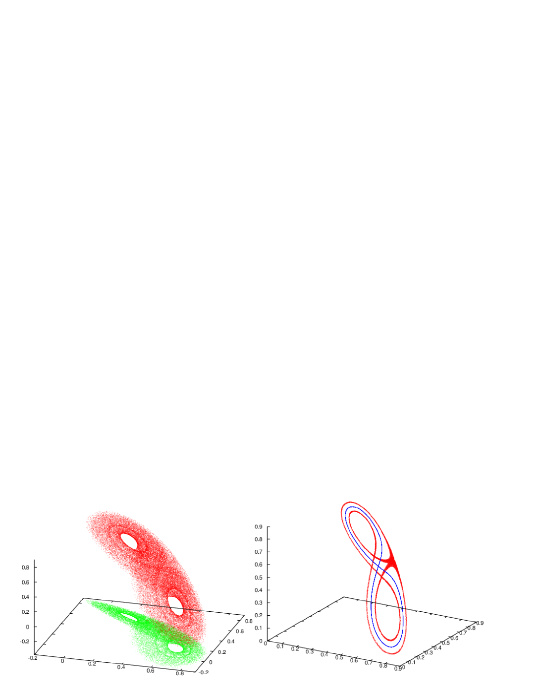
Figure 1: Plots of attractors of map (1.1) observed numerically in [1] for $M_{1}=0,B=0.7$ and $M_{2}=0.85$ (left) or $M_{2}=0.815$ (right). In the left panel, the projection on the $(x,y)$-plane is also displayed. In the right panel, a ’’figure-eight’’ saddle closed invariant curve inside the lacuna is shown. Note the similarity to the Lorenz attractors of the Shimizu-Morioka system, see [54, 55, 56].

The similarity between the discrete and classical Lorenz attractors appears to be not accidental and it can be explained by various reasons. Thus, it is well known that the classical Lorenz attractor can be born as a result of local bifurcations of an equilibrium state with three zero eigenvalues when a flow possesses a (Lorenzian) symmetry [45]. Analogously for maps, discrete Lorenz attractors can arise under bifurcations of fixed points with multipliers $(-1,-1,+1)$, in this case the required local symmetry exists automatically due to negative multipliers. As it was shown in [1, 41], the second iteration of the map near this point can be embedded into a flow up to asymptotically small periodic non-autonomous terms. The corresponding flow normal form of such bifurcations coincides with the well-known Shimizu-Morioka model, which, in turn, exhibits the Lorenz attractor for certain parameter values [39, 50]. Thus, we can consider the attractor in the map as the one of the Poincaré map (period map) of a periodically perturbed system with the Lorenz attractor. On the other hand, as it was shown in paper [42] by Turaev and Shilnikov, such discrete attractor is genuine in the sense that every its orbit has positive maximal Lyapunov exponent.

In the present paper we study bifurcations of three-dimensional diffeomorphisms with homoclinic tangencies, leading to the birth of descrete Lorenz attractors. Problems of this kind were previously analyzed in [43, 46, 47, 48, 4].

In [46, 47, 48] the birth of discrete Lorenz attractors from nontransversal heteroclinic cycles of three-dimensional diffeomorphisms was studied. Such a cycle contains two fixed points $O_{1}$ and $O_{2}$ of type (2,1), i.e. with $\dim W^{s}(O_{i})=2,\dim W^{u}(O_{i})=1$, and one pair of stable and unstable manifolds intersect transversely and another pair has a quadratic tangency. It was assumed that at least one of the points $O_{1}$ and $O_{2}$ is a saddle-focus, see Fig. Moreover, in all cases the additional condition that the Jacobians of the map in points $O_{1}$ and $O_{2}$ are greater and less than one respectively was imposed (the so-called case of contracting-expanding maps). The birth of discrete Lorenz attractors was proved for three-parameter general unfoldings.

Remark. Naturally, three parameters are needed to allow generically the existence of triply degenerate fixed points in the corresponding first return maps. In such families the first return map can be rescaled to the form asymptotically close to map (1.1). Thus, using the results of [1] (see also [41] for more generic statement), we deduce the birth of discrete Lorenz attractors in close systems.

In the case of homoclinic tangencies to the saddle fixed point $O$ of a three-dimensional diffeomorphism $T$ the birth of Lorenz attractors was proved in the cases when:

1) [43], the point $O$ is a saddle-focus with the unit Jacobian (saddle-focus of conservative type).

2) [4], the fixed point is a saddle with the unit Jacobian and the quadratic tangency is non-simple.

We note that the condition on Jacobians in all these cases is necessary for the existence of a non-trivial (three-dimensional) dynamics in the neighborhood of the homoclinic orbit [14]. Otherwise, if, for example, one has $J<1$, all three-dimensional volumes will be contracted under the iterations of map $T$ (near point $O$) and, hence, the dynamics of first return maps $T^{k}$ for large $k$ will be effectively two-dimensional, or even one-dimensional. Recall that, by definition [14], the effective dimension $d_{e}$ of a bifurcation problem equals $n$, if periodic orbits with $n$ multipliers equal $\pm 1$ can appear at bifurcations but no orbits exist with more than $n$ unit multipliers.

Formally, if to consider three-dimensional diffeomorphisms with homoclinic tangencies to a hyperbolic saddle fixed point with $|J|=1$, then $d_{e}$ can be equal to $3$ only in the following cases: (i) the point is a saddle-focus; (ii) the point is the saddle (all multipliers are real) and the tangency is not simple, and (iii) the point is a resonant saddle, i.e. it has two multipliers equal in the absolute value. Otherwise, the effective dimension is less than three since the direction of strong contraction is present [12, 3] for all nearby systems.

Cases (i) and (ii) were considered in [43] and [4] respectively. In this paper we consider the new case (iii) when the saddle is resonant. Note that if the resonance $\lambda_{1}=\lambda_{2}$ takes place, we may perturb the map in such a way that the resulting map will have a saddle-focus fixed point with $|J|=1$ and, hence, we can apply results of [43] to prove the birth of discrete Lorenz attractors. It not the case for the resonance $\lambda_{1}=-\lambda_{2}$ which is of independent interest.

We consider the case when a fixed point $O$ has multipliers $\lambda,-\lambda,\gamma$ such that $0<\lambda<1$, $|\gamma|>1$ and $|\lambda^{2}\gamma|=1$. This means that $O$ is a resonant saddle point of conservative type. Obviously, the bifurcation codimension of this problem is at least three and, as we will show, $d_{e}=3$ in this case.

We show that in the three-parametric families $f_{\mu}$, $\mu=(\mu_{1},\mu_{2},\mu_{3})$ unfolding generally this type of a homoclinic tangency, in the parameter space there exist domains $\triangle_{k}\to\{\mu=0\}$ as $k\to\infty$ such that for $\mu\in\triangle_{k}$ the first return map $T_{k}$ possesses the discrete Lorenz attractor. Recall that the map $T_{k}$ is constructed by the iterations of map $f_{\mu}$, i.e. $T_{k}=f_{\mu}^{k}$, but the domain of its definition is a small box $\sigma_{0}^{k}$ near some homoclinic point.

The paper consists of two paragraphs. In §2 we formulate our main result – Theorem 2.13 and construct the first return map of some small neighborhood of the homoclinic orbit. In §3 we prove Theorem 2.13.

2 Statement of the problem and formulation of main results.

We study bifurcations of three-dimensional diffeomorphisms of a special type (codimension two) quadratic homoclinic tangency to a saddle fixed point with the unit Jacobian. Namely, we assume that the initial diffeomorphism $f_{0}\in C^{r},r\geq 5,$ satisfies the following conditions:

1. $f$ has a saddle fixed point $O$ with real multipliers $\lambda_{1},\lambda_{2},\gamma$ such that $0<|\lambda_{1,2}|<1<|\gamma|$ and

   $$J_{0}\equiv|\lambda_{1}\lambda_{2}\gamma|=1.$$

2. The stable $W^{s}(O)$ and unstable $W^{u}(O)$ invariant manifolds of $O$ have a quadratic tangency at the points of some homoclinic orbit $\Gamma_{0}$.

3. The saddle $O$ is resonant in the sense that $\lambda_{1}=-\lambda_{2}=\lambda>0$.

Condition A means that the point $O$ is a saddle of conservative type and $\dim\;W^{s}(O)=2$ and $\dim\;W^{u}(O)=1$. Condition C is an additional degeneracy of the saddle fixed point. We will consider smooth parameter families $f_{\varepsilon}$ of diffeomorphisms (general unfoldings of conditions A–C), such that $f_{0}$ belongs to it for $\varepsilon=0$.

Let $U\equiv U(O\cup\Gamma_{0})$ be a sufficiently small fixed neighbourhood of $\Gamma_{0}$ that is a union of a neighbourhood $U_{0}$ of $O$ and a number of neighbourhoods of those points of $\Gamma_{0}$ which lie outside $U_{0}$. Denote by $T_{0}$ the restriction of the diffeomorphism $f_{\varepsilon}$ onto $U_{0}$. We call $T_{0}$ a local map. By a linear transformation of coordinates in $U_{0}$, map $T_{0}$ can be written as

$$(\bar{x}_{1},\bar{x}_{2},\bar{y})=(\lambda_{1}x_{1},\lambda_{2}x_{2},\gamma y)\;+\;h.o.t.$$

The origin $O=(0,0,0)$ is a fixed point of $T_{0}$, the stable manifold $W^{s}(O)$ is tangent at $O$ to the $(x_{1},x_{2})$-plane and the unstable manifold $W^{u}(O)$ is tangent at $O$ to the $y$-axis. The intersection points of $\Gamma_{0}$ with $U_{0}$ belong to the set $W^{s}\cap W^{u}$ and accumulate to $O$ at both forward and backward iterations. Thus, infinitely many points of $\Gamma_{0}$ lie on $W^{s}_{loc}$ and $W^{u}_{loc}$. Let $M^{+}\in W^{s}_{loc}$ and $M^{-}\in W^{u}_{loc}$ be two such points and let $M^{+}=f_{0}^{n_{0}}(M^{-})$ for some positive integer $n_{0}$. Let $\Pi^{+}\subset U_{0}$ and $\Pi^{-}\subset U_{0}$ be small neighbourhoods of points $M^{+}$ and $M^{-}$ respectively. The map $T_{1}\equiv f_{\varepsilon}^{n_{0}}:\Pi^{-}\rightarrow\Pi^{+}$ is called a global map.

From [32, 27, 28, 22] it is known that there exists a $C^{r}$-change of coordinates (which is $C^{r-2}$-smooth in the parameters) bringing $T_{0}$ to the so-called main normal form:

$$\begin{array}[]{l}\bar{x}_{1}\;=\;\lambda_{1}(\varepsilon)x_{1}+O(\|x\|^{2}|y|)\;,\\ \bar{x}_{2}\;=\;\lambda_{2}(\varepsilon)x_{2}+O(\|x\|^{2}|y|)\;,\\ \bar{y}\;=\;\gamma(\varepsilon)y+O(\|x\||y|^{2})\;.\\ \end{array}$$ (2.1)

The main peculiarity of this form is that in coordinates (2.1) the stable and unstable manifolds of the saddle fixed point are locally straightened, their equations are $W^{s}:\{y=0\}$, $W^{u}:\{x_{1}=0,x_{2}=0\}$. The main normal form also allows to obtain a quite simple representation of the iterations of $T_{0}$. The latter can be formulated as the following lemma:

Lemma 1

[3] For any positive integer $k$ and for any sufficiently small $\varepsilon$ the map $T_{0}^{k}(\varepsilon)\;:\;(x_{0},y_{0})\;\to\;(x_{k},y_{k})$ can be written in the following cross-form

$$\begin{array}[]{l}x_{k1}\;-\;\lambda_{1}^{k}(\varepsilon)x_{01}\;=\;\hat{\lambda}^{k}\xi_{k1}(x_{0},y_{k},\varepsilon)\;,\\ x_{k2}\;-\;\lambda_{2}^{k}(\varepsilon)x_{02}\;=\;\hat{\lambda}^{k}\xi_{k2}(x_{0},y_{k},\varepsilon)\;,\\ y_{0}\;-\;\gamma(\varepsilon)^{-k}y_{k}\;=\;\hat{\gamma}^{-k}\eta_{k}(x_{0},y_{k},\varepsilon)\;\;,\end{array}$$ (2.2)

where $\hat{\lambda}$ and $\hat{\gamma}$ are some constants such that $\hat{\lambda}=\lambda+\delta,\;\hat{\gamma}=\lambda|\gamma^{-1}|-\delta$ for some small $\delta>0$ and functions $\xi_{k}$ and $\eta_{k}$ are uniformly bounded along with all derivatives up to order $(r-2)$.

Next we construct the most appropriate form for the global map $T_{1}$ for all small $\varepsilon$. Let the chosen homoclinic points have coordinates $M^{+}=M^{+}(x_{1}^{+},x_{2}^{+},0)\in W^{s}_{loc}$ and $M^{-}=M^{-}(0,0,y^{-})\in W^{u}_{loc}$, where $(x_{1}^{+})^{2}+(x_{2}^{+})^{2}\neq 0$ and $y^{-}>0$. At $\varepsilon=0$ we have that $T_{1}M^{-}=M^{+}$ and $T_{1}(W_{loc}^{u})$ and $W_{loc}^{s}$ are tangent quadratically at the point $M^{+}$. Thus, the global map $T_{1}$ at $\varepsilon=0$ can be written as the Taylor expansion near the point $(x_{1}=0,x_{2}=0,y=y^{-}$):

$$\begin{array}[]{l}\bar{x}_{1}-x_{1}^{+}\;=\;a_{11}x_{1}+a_{12}x_{2}+b_{1}(y-y^{-})+O(\|x\|^{2})+O(\|x\||y-y^{-}|)+O((y-y^{-})^{2})\\ \bar{x}_{2}-x_{2}^{+}\;=\;a_{21}x_{1}+a_{22}x_{2}+b_{2}(y-y^{-})+O(\|x\|^{2})+O(\|x\||y-y^{-}|)+O((y-y^{-})^{2})\\ \bar{y}\;=\;c_{1}x_{1}+c_{2}x_{2}+d(y-y^{-})^{2}+O(\|x\|^{2})+O(\|x\||y-y^{-}|)+O(|y-y^{-}|^{3})\end{array}$$ (2.3)

The equation of curve $T_{1}(W^{u}_{loc})$ at $\varepsilon=0$ looks as follows (we put $x_{1}=x_{2}=0$ in (2.3)):

$$\begin{array}[]{l}\bar{x}_{1}-x_{1}^{+}\;=\;b_{1}(y-y^{-})+O((y-y^{-})^{2})\\ \bar{x}_{2}-x_{2}^{+}\;=\;b_{2}(y-y^{-})+O((y-y^{-})^{2})\\ \bar{y}\;=\;d(y-y^{-})^{2}+O(|y-y^{-}|^{3})\\ \end{array}$$ (2.4)

This is a parametric equation (with parameter $(y-y^{-})$) of the curve $T_{1}(W^{u}_{loc})$ in a neighbourhood of $M^{+}$. The equation of $W^{s}_{loc}$ is $y=0$. Since the initial homoclinic tangency is quadratic, it follows that $d\neq 0,\;b_{1}^{2}+b_{2}^{2}\neq 0$. Moreover, map $T_{1}(0)$ is a diffeomorphism, therefore

$$J_{1}={\rm det}\;\left(\begin{array}[]{rcl}a_{11}&a_{12}&\;b_{1}\\ a_{21}&a_{22}&\;b_{2}\\ c_{1}&c_{2}&\;0\\ \end{array}\right)\neq 0$$ (2.5)

and, hence, $c_{1}^{2}+c_{2}^{2}\neq 0$.

At small $\varepsilon$ the global map $T_{1}(\varepsilon)$ can be written in the following form (the Taylor expansion near the point $(x_{1},x_{2},y)=(0,0,y^{-}(\varepsilon))$

$$\begin{array}[]{l}\bar{x}_{1}-x_{1}^{+}(\varepsilon)\;=\;a_{11}x_{1}+a_{12}x_{2}+b_{1}(y-y^{-}(\varepsilon))+\ldots\\ \bar{x}_{2}-x_{2}^{+}(\varepsilon)\;=\;a_{21}x_{1}+a_{22}x_{2}+b_{2}(y-y^{-}(\varepsilon))+\ldots\\ \bar{y}\;=\;y^{+}(\varepsilon)+c_{1}x_{1}+c_{2}x_{2}+d(y-y^{-}(\varepsilon))^{2}+\ldots\\ \end{array}$$ (2.6)

where $x_{1}^{+}(0)=x_{1}^{+},x_{2}^{+}(0)=x_{2}^{+},y^{-}(0)=y^{-},y^{+}(0)=0$; all coefficients $a_{11},\ldots,d$ depend (smoothly) on $\varepsilon$; and we shift $y^{-}$ into $y^{-}(\varepsilon)$ in order to nullify the linear in $y$ terms from the right side of the third equation.

We assume that the following general condition holds

$$b_{1}c_{1}b_{2}c_{2}\neq 0.$$ (2.7)

Its meaning is as follows: if at least one of these four coefficients is zero, then in any neighborhood of $f_{0}$ there exist maps having a nontransversal homoclinic orbit close to $\Gamma_{0}$ with a non-simple quadratic tangency (see [2, 6, 4] for details); it composes an additional degeneracy which we do not consider here.

Conditions A, B, C together with (2.7) define a codimension $3$ bifurcation surfaces of diffeomorphisms with a quadratic homoclinic tangency. Hence, as a general unfolding we should consider a three-parameter families where the parameters $\mu_{1},\mu_{2}$ and $\mu_{3}$ control the degeneracies imposed due to conditions B, A and C, respectively.

Naturally, the splitting distance of manifolds $W^{s}(O)$ and $W^{u}(O)$ with respect to the point $M^{+}$ is considered as the first governing parameter $\mu_{1}$. It is seen from (2.6) that

$$\;\;\mu_{1}\equiv y^{+}(\varepsilon)\;.$$ (2.8)

The second parameter should control the Jacobian $J=\lambda_{1}\lambda_{2}\gamma$ of $f_{\mu}$ at saddle $O_{\mu}$. Therefore, we define

$$\;\mu_{2}=1-|\lambda_{1}\lambda_{2}\gamma|$$ (2.9)

As the third parameter $\mu_{3}$ we consider the value that controls the difference between $|\lambda_{1}|$ and $|\lambda_{2}|$, namely:

$$\;\mu_{3}=\frac{|\lambda_{1}(\varepsilon)|}{|\lambda_{2}(\varepsilon)|}-1$$ (2.10)

Thus, the family $f_{\mu_{1},\mu_{2},\mu_{3}}$ constructed above can be considered as a general unfolding of the corresponding homoclinic tangency to a resonant saddle, satisfying conditions A, B and C.

Now we are able to construct the first return maps $T_{k}$ using formulae (2.2) and (2.6). As a result we will obtain a formula for $T_{k}$ in the initial (small) variables $(x_{1},x_{2},y)\in U_{0}$ and parameters $\mu_{1}$, $\mu_{2}$ and $\mu_{3}$. Next, we rescale the initial variables and parameters

$$(x_{1},x_{2},y)\mapsto(X_{1},X_{2},Y)\;,\;(\mu_{1},\mu_{2},\mu_{3})\mapsto(M_{1},M_{2},M_{3})\;,$$

with asymptotically small (as $k\to\infty$) factors, in such a way that in the rescaled variables and parameters map $T_{k}$ is rewritten as some three-dimensional quadratic map which contains asymptotically small (as $k\to\infty$) terms. Moreover, new coordinates $(X_{1},X_{2},Y)$ and parameters $(M_{1},M_{2},M_{3})$ can take arbitrary finite values at large $k$ (i.e. covering all values in the limit $k\to\infty$).

Our main result is the following theorem.

Theorem 1

Let $f_{\mu_{1},\mu_{2},\mu_{3}}$ be the family under consideration. Then, in the $(\mu_{1},\mu_{2},\mu_{3})$-parameter space, there exist infinitely many regions $\Delta_{k}$ accumulating at the origin as $k\to\infty$ such that the map $T_{k}$ in appropriate rescaled coordinates and parameters is asymptotically $C^{r-1}$-close to the following limit map

$$\begin{array}[]{l}\displaystyle\bar{X}_{1}\;=\;Y,\;\;\bar{X}_{2}\;=X_{1},\;\;\bar{Y}=M_{1}+M_{2}X_{1}+BX_{2}-Y^{2}\;,\end{array}$$ (2.11)

where

$$\begin{array}[]{l}M_{1}\;=\;-d\gamma^{2k}[\mu_{1}+\lambda_{1}^{k}c_{1}x_{1}^{+}+\lambda_{2}^{k}c_{2}x_{2}^{+}+o(\lambda^{k})]\end{array}$$ (2.12)

and

$$\begin{array}[]{l}\displaystyle M_{2}=\left(b_{1}c_{1}+b_{2}c_{2}\frac{\lambda_{2}^{k}}{\lambda_{1}^{k}}\right)\lambda_{1}^{k}\gamma^{k}(1+\dots),\;\;B=J_{1}(\lambda_{1}\lambda_{2}\gamma)^{k}(1+\dots)\end{array}$$ (2.13)

3 Proof of Theorem 2.13.

Using (2.6) and (2.2) one can write the map $T_{k}=T_{1}T_{0}^{k}$ for sufficiently large $k$ and small $\varepsilon$ in the form

$$\begin{array}[]{l}\bar{x}_{1}-x_{1}^{+}\;=\;a_{11}(\lambda_{1}^{k}x_{1}+\hat{\lambda}^{k}\xi_{k1}(x,y,\varepsilon))+a_{12}(\lambda_{2}^{k}x_{2}+\hat{\lambda}^{k}\xi_{k2}(x,y,\varepsilon))+\\ \qquad+b_{1}(y-y^{-})+O(|y-y^{-}|^{2}+\lambda^{k}\|x\||y-y^{-}|)+\lambda^{2k}\|x\|^{2})\;,\\ \\ \bar{x}_{2}-x_{2}^{+}\;=\;a_{12}(\lambda_{1}^{k}x_{1}+\hat{\lambda}^{k}\xi_{k1}(x,y,\varepsilon))+a_{22}(\lambda_{2}^{k}x_{2}+\hat{\lambda}^{k}\xi_{k2}(x,y,\varepsilon))+\\ \qquad+b_{2}(y-y^{-})+O(|y-y^{-}|^{2}+\lambda^{k}\|x\||y-y^{-}|)+\lambda^{2k}\|x\|^{2})\;,\\ \\ \gamma^{-k}\bar{y}-\hat{\gamma}^{-k}\eta_{k}(\bar{x},\bar{y},\varepsilon)\;=\;\mu_{1}+c_{1}(\lambda_{1}^{k}x_{1}+\hat{\lambda}^{k}\xi_{k1}(x,y,\varepsilon))+\\ \qquad+c_{2}(\lambda_{2}^{k}x_{2}+\hat{\lambda}^{k}\xi_{k2}(x,y,\varepsilon))+d(y-y^{-})^{2}+\\ \qquad+O(|y-y^{-}|^{3}+\lambda^{k}\|x\||y-y^{-}|+\lambda^{2k}\|x\|^{2})\;.\\ \end{array}$$ (3.1)

We shift coordinates $x_{1new}\;=\;x_{1}-x_{1}^{+}+\phi_{k}^{1}(\varepsilon),\;x_{2new}\;=\;x_{2}-x_{2}^{+}+\phi_{k}^{2}(\varepsilon),\;y_{new}\;=\;y-y^{-}+\psi_{k}(\varepsilon)$, where $\phi_{k},\psi_{k}=O(\lambda^{k})$, in such a way that the right sides of (3.1) do not contain constant terms for the first two equations and linear in $y_{new}$ terms for the third equation. Then (3.1) takes the form

$$\begin{array}[]{l}\bar{x}_{1}\;=\;a_{11}\lambda_{1}^{k}x_{1}+a_{12}\lambda_{2}^{k}x_{2}+b_{1}y+O(y^{2}+\lambda^{k}\|x\||y|+\hat{\lambda}^{k}\|x\|^{2})\;,\\ \\ \bar{x}_{2}\;=\;a_{21}\lambda_{1}^{k}x_{1}+a_{22}\lambda_{2}^{k}x_{2}+b_{2}y+O(y^{2}+\lambda^{k}\|x\||y|+\hat{\lambda}^{k}\|x\|^{2})\;,\\ \\ \bar{y}-(\hat{\gamma}/\gamma)^{-k}\eta_{k}(\bar{x}+x^{+}+\phi_{k},\bar{y}+y^{-}+\psi_{k},\varepsilon)\;=\;M_{k}+\\ \qquad d\gamma^{k}y^{2}+\lambda_{1}^{k}\gamma^{k}c_{1}x_{1}+\lambda_{2}^{k}\gamma^{k}c_{2}x_{2}+\gamma^{k}O(|y|^{3}+\lambda^{k}\|x\||y|)+\hat{\lambda}^{k}\|x\|^{2})\par\par\end{array}$$ (3.2)

where

$$\begin{array}[]{l}M_{k}\;=\;\gamma^{k}[\mu_{1}+\lambda_{1}^{k}c_{1}x_{1}^{+}+\lambda_{2}^{k}c_{2}x_{2}^{+}+o(\lambda^{k})]\end{array}$$ (3.3)

Consider the third equation of (3.2). First of all, we transform its left side. Namely, we write $\bar{y}-(\hat{\gamma}/\gamma)^{-k}\eta_{k}=\bar{y}+(\hat{\gamma}/\gamma)^{-k}[\eta_{k}^{0}+\eta_{k}^{1}(\bar{x},\varepsilon)+\eta_{k}^{2}(\bar{y},\varepsilon)+\eta_{k}^{3}(\bar{x},\bar{y},\varepsilon)]$ where $\eta_{k}^{1}(0,\varepsilon)=0$, $\eta_{k}^{2}(0,\varepsilon)=0$ and $\eta_{k}^{3}=O(\|\bar{x}\bar{y}\|)$. Next, we transfer constant term $(\hat{\gamma}/\gamma)^{-k}\eta_{k}^{0}$ into the right side and join it to $M_{k}^{1}$; we substitute the value of $\bar{x}$ due to the first two equations of (3.2) into function $\eta_{k}^{1}(\bar{x},\varepsilon)$ and transfer the obtained expression into the right side. After this, all coefficients (in the third equation) get additions of order $O(\hat{\gamma}^{-k})$ and a new linear term in $y$, $p_{k}y=O([\hat{\gamma}/\gamma]^{-k})y$, appears. By the shift of coordinates of the form $(x,y)\mapsto(x,y)+O([\hat{\gamma}/\gamma]^{-k})$, we vanish both this linear term and constant terms in the right sides of the first and second equations. As the result, the left side of the third equation can be written as follows:

$$\bar{y}+(\hat{\gamma}/\gamma)^{-k}O(\bar{y})+(\hat{\gamma}/\gamma)^{-k}O(\|\bar{x}\bar{y}\|)=\bar{y}(1+q_{k})+(\hat{\gamma}/\gamma)^{-k}O(\bar{y}^{2})+(\hat{\gamma}/\gamma)^{-k}O(\|\bar{x}\bar{y}\|)$$

where $q_{k}=O([\hat{\gamma}/\gamma]^{-k})$. After this, we can write system (3.2) in the form

$$\begin{array}[]{l}\bar{x}_{1}\;=\;a_{11}\lambda_{1}^{k}x_{1}+a_{12}\lambda_{2}^{k}x_{2}+b_{1}y+O(y^{2})+\lambda^{k}O(\|x\||y|)+\hat{\lambda}^{k}O(\|x\|^{2})\;,\\ \bar{x}_{2}\;=\;a_{21}\lambda_{1}^{k}x_{1}+a_{22}\lambda_{2}^{k}x_{2}+b_{2}y+O(y^{2})+\lambda^{k}O(\|x\||y|)+\hat{\lambda}^{k}O(\|x\|^{2})\;,\\ \\ \bar{y}(1+q_{k})+(\hat{\gamma}/\gamma)^{-k}O(|\bar{y}|^{2})+(\hat{\gamma}/\gamma)^{-k}O(\|\bar{x}\bar{y}\|)\;=\;M_{k}+\\ \qquad+d\gamma^{k}(1+s_{k})y^{2}+c_{1}\lambda_{1}^{k}\gamma^{k}x_{1}+c_{2}\lambda_{2}^{k}\gamma^{k}x_{2}+p_{k}\gamma^{k}O(\|x\|^{2})+\\ \qquad+\lambda^{k}\gamma^{k}O(\|x\||y|)+\gamma^{k}O(y^{3})\;,\\ \end{array}$$ (3.4)

where $s_{k}=O(\lambda^{k}+|\hat{\gamma}/\gamma|^{-k})$, $p_{k}=O(\hat{\lambda}^{k}+|\hat{\gamma}/\gamma|^{-k})$ and new $M_{k}$ satisfies (3.3).

We perform a linear change of $x$ variables to make zero the linear in $y$ term in the second equation:

$$x_{2new}=x_{2}-\frac{b_{2}}{b_{1}}x_{1},\;x_{1new}=x_{1}\;,\;y_{new}=y.$$

Then (3.4) is rewritten in the form

$$\begin{array}[]{l}\displaystyle\bar{x}_{1}\;=\;b_{1}y+\lambda^{k}O(\|x\|)+O(y^{2})\;,\\ \\ \displaystyle\bar{x}_{2}=A_{21}\lambda_{1}^{k}x_{1}+A_{22}\lambda_{2}^{k}x_{2}+O(y^{2})+\lambda^{k}O(\|x\||y|)+\lambda^{2k}O(\|x\|^{2})\;,\\ \\ \bar{y}(1+q_{k})+(\hat{\gamma}/\gamma)^{-k}O(|\bar{y}|^{2}+\|\bar{x}\bar{y}\|)\;=\;M_{k}+\lambda_{1}^{k}\gamma^{k}c_{1}\nu_{k}x_{1}+\lambda_{2}^{k}\gamma^{k}c_{2}x_{2}+d\gamma^{k}(1+s_{k})y^{2}+\\ \qquad\qquad p_{k}\gamma^{k}O(\|x\|^{2})+\lambda^{k}\gamma^{k}O(\|x\||y|)+\par\gamma^{k}O(y^{3})\;,\end{array}$$ (3.5)

where

$$\begin{array}[]{c}\displaystyle A_{21}=\left(a_{21}-\frac{b_{2}}{b_{1}}a_{11}\right)+\left(a_{22}-\frac{b_{2}}{b_{1}}a_{12}\right)\frac{b_{2}}{b_{1}}\frac{\lambda_{2}^{k}}{\lambda_{1}^{k}},\\ \displaystyle A_{22}=a_{22}-\frac{b_{2}}{b_{1}}a_{12},\\ \displaystyle\nu_{k}=\left(1+\frac{b_{2}c_{2}}{b_{1}c_{1}}\frac{\lambda_{2}^{k}}{\lambda_{1}^{k}}\right).\end{array}$$ (3.6)

Now we will vary $\lambda_{1}$ and $\lambda_{2}$ in such a way that the value of $\nu_{k}$ is asymptotically small as $k\to\infty$. This is always possible via small changes of parameter $\mu_{3}$ because $b_{1}c_{1}\neq 0$ and $b_{2}c_{2}\neq 0$ and $\lambda_{1}=-\lambda_{2}$ in the initial moment. Then it is clear that

$$A_{21}=\frac{J_{1}}{c_{2}b_{1}}+O(\nu_{k})\neq 0,$$

where $J_{1}$ is given by formula (2.5).

Rescale the coordinates as follows

$$y=-\frac{\gamma^{-k}(1+q_{k})}{d(1+s_{k})}\;Y\;,\;x_{1}=-\frac{b_{1}\gamma^{-k}(1+q_{k})}{d(1+s_{k})}\;X_{1}\;,\;x_{2}=-\frac{b_{1}A_{21}\gamma^{-k}\lambda_{1}^{k}(1+q_{k})}{d(1+s_{k})}\;X_{2}.$$

Then system (3.5) is rewritten in the new coordinates as follows

$$\begin{array}[]{l}\displaystyle\bar{X}_{1}\;=\;Y+O(\lambda^{k})\;,\\ \bar{X}_{2}\;=\;X_{1}+O(\gamma^{-k}\lambda^{-k})\;,\\ \bar{Y}=M_{1}+M_{2}X_{1}+BX_{2}-Y^{2}+O(\gamma^{-k}\lambda^{-k})\;,\end{array}$$ (3.7)

where formulas (2.12) and (2.13) are valid for $M_{1}$, $M_{2}$ and $B$.

It is obvious that system (3.7) is asymptotically close to (2.11) when $k\to\infty$. $\;\;\;\Box$.

References

- [1] Gonchenko S. V., Ovsyannikov I. I., Simó C. and Turaev D. 2005 Three-dimensional Hénon-like maps and wild Lorenz-like attractors. Bifurc. Chaos 15 3493–3508
- [2] J.C.Tatjer. Three-dimensional dissipative diffeomorphisms with homoclinic tangencies. Ergod.Th. & Dynam.Sys. 2001. V.21. P.249–302.
- [3] S.V.Gonchenko, L.P.Shilnikov, D.V.Turaev. On dynamical properties of multidimensional diffeomorphisms from Newhouse regions. Nonlinearity, 2008, vol. 21, pp. 923–972.
- [4] S.V.Gonchenko, I.I.Ovsyannikov, J.C.Tatjer. Birth of Discrete Lorenz Attractors at the Bifurcations of 3D Maps with Homoclinic Tangencies to Saddle Points. Regular and Chaotic Dynamics, 2014, Vol. 19, No. 4, pp. 495-?505.
- [5] Newhouse S.E., Palis J., Takens F. Bifurcations and stability of families of diffeomorphisms. Publ.Math.Inst. Haute Etudes Scientifiques, 1983, v., 5–72.
- [6] S.V.Gonchenko, V.S.Gonchenko, J.C.Tatjer. Bifurcations of three-dimensional diffeomorphisms with non-simple quadratic homoclinic tangencies and generalized Henon maps. Regular and Chaotic Dynamics. 2007. V.12. No.3, 233–266.
- [7] D.V.Turaev, L.P.Shilnikov. An example of a wild strange attractor. Sb. Math. 1998. V.189. No.2. P.137–160.
- [8] N.K.Gavrilov, L.P.Shilnikov. On three-dimensional dynamical systems close to systems with a structurally unstable homoclinic curve. Part 1. Math.USSR Sb. 1972. V.17. P.467–485 ; Part 2. Math.USSR Sb. 1973. V.19. P.139–156.
- [9] S.Newhouse. Diffeomorphisms with infinitely many sinks. Topology. 1974. V.13. P.9–18.
- [10] S.V.Gonchenko. On stable periodic motions in systems close to a system with a nontransversal homoclinic curve. Russian Math. Notes. 1983. V.33. No.5. P.384–389.
- [11] J.C.Tatjer, C.Simó. Basins of attraction near homoclinic tangencies. Erg.Th. & Dynam.Sys. 1994. V.14. No.2. P.351–390.
- [12] S.V.Gonchenko, L.P.Shilnikov, D.V.Turaev. Dynamical phenomena in systems with structurally unstable Poincare homoclinic orbits. Russian Acad. Sci. Dokl. Math. 1993. V.47. No.3. P.410–415.
- [13] S.V.Gonchenko, L.P.Shilnikov, D.V.Turaev. Dynamical phenomena in systems with structurally unstable Poincare homoclinic orbits. Interdisc. J. CHAOS. 1996. V.6. No.1. P.15–31.
- [14] D.V.Turaev. On dimension of nonlocal bifurcational problems. Int.J. of Bifurcation and Chaos. 1996. V.6. No.5. P.919–948.
- [15] S.V.Gonchenko, L.P.Shilnikov, D.V.Turaev. Homoclinic tangencies of an arbitrary order in Newhouse domains. Itogi Nauki Tekh., Ser. Sovrem. Mat. Prilozh., Temat. Obz. 1999. V.67. P.69–128. // English transl. in J.Math.Sci. New York. 2001. V.105. No.1. P.1738–1778.
- [16] H.Broer, C.Simó, J.C.Tatjer. Towards global models near homoclinic tangencies of dissipative diffeomorphisms. Nonlinearity. 1998. V.11. No.3. P.667–770.
- [17] S.V.Gonchenko, V.S.Gonchenko. On Andronov-Hopf bifurcations of two-dimensional diffeomorphisms with homoclinic tangencies. WIAS-Preprint No.556. Berlin. 2000.
- [18] S.V.Gonchenko, V.S.Gonchenko. On bifurcations of birth of closed invariant curves in the case of two-dimensional diffeomorphisms with homoclinic tangencies. Proc. of Math.Steklov Inst. 2004. v.244.
- [19] L.Tedeschini-Lalli, J.A.Yorke. How often do simple dynamical processes have infinitely many coexisting sinks? Commun.Math.Phys. 1986. V.106. P.635–657.
- [20] V.S.Biragov. On bifurcations in a two-parameter family of conservative maps close to the Hénon map. Methods of the Qualitative Theory of Differential Equations: E.A.Leontovich-Andronova Ed., Gorky State Univ. 1987. P.10–23.// English transl. in Selecta Math. Sovietica. 1990. V.9.
- [21] S.V.Gonchenko, L.P.Shilnikov, D.V.Turaev. On dynamical properties of diffeomorphisms with homoclinic tangencies. Contemporary Mathematics and its Applications. 2003. V.7. P.92–118 (in Russian) [English version is in: J. Math. Sci. (N.Y.). 2005. V.126. P.1317–1343.]
- [22] S.V.Gonchenko, L.P.Shilnikov, D.V.Turaev. Homoclinic tangencies of arbitrarily high orders in conservative and dissipative two-dimensional maps. Nonlinearity, 20 (2007), 241–275.
- [23] C.E.Frouzakis, L.Gardini, I.G.Kevrekidis, G.Millerioux, C.Mira. On some properties of invariant sets of two-dimensional noninvertible maps. Int. J. of Bifurcation and Chaos. 1997. V.7. No.6.
- [24] C.Mira, L.Gardini, A.Barugola, J.C.Cathala. Chaotic dynamics in two-dimensional noninvertible maps. World Scientific, Singapore. 1966.
- [25] A.Pumariño, J.C.Tatjer. Dynamics near homoclinic bifurcations of three-dimensional dissipative diffeomorphisms. Nonlinearity. 2006. V.19. P.2833–2852.
- [26] A.Pumariño, J.C.Tatjer. Attractors for return maps near homoclinic tangencies of three-dimensional dissipative diffeomorphisms. Preprint 2007.
- [27] S.V.Gonchenko, L.P.Shilnikov. Invariants of -conjugacy of diffeomorphisms with a nontransversal homoclinic orbit. Ukr.Math.J. 1990. V.42. No.2. P.134–140.
- [28] S.V.Gonchenko, L.P.Shilnikov. On moduli of systems with a nontransversal Poincare homoclinic orbit. Russian Acad.Sci.Izv.Math. 1993. V.41. No.3. P.417–445.
- [29] V.S.Gonchenko, Yu.A.Kuznetsov, H.G.E.Meijer. Generalized Hénon map and bifurcations of homoclinic tangencies. SIAM J. of Appl. Dyn. Sys. 2005. V.4. No.2. P.407–436.
- [30] V.S.Gonchenko. On bifurcations of two-dimensional diffeomorphisms with a homoclinic tangency of manifolds of a ’’neutral’’ saddle. Proc. of Math. Steklov Inst. 2002. V.236. P.86–93.
- [31] M.W.Hirsch, C.C.Pugh, M.Shub. Invariant manifolds. Lecture Notes in Math. 1977. V.583, Springer-Verlag, Berlin.
- [32] L.P.Shilnikov, A.L.Shilnikov, D.V.Turaev and L.O.Chua. Methods of Qualitative Theory in Nonlinear Dynamics, Part I. World Scientific. 1998.
- [33] J.Palis, M.Viana. High dimension diffeomorphisms displaying infinitely many periodic attractors. Ann. Math. 1994. V.140. P.207–250.
- [34] V.S.Gonchenko, I.I.Ovsyannikov. On bifurcations of three-dimensional diffeomorphisms with a homoclinic tangency to a ’’neutral’’ saddle fixed point. Proceedings of S.Petersburg Steklov Math.Inst. 2003. V.300. P.167–172.
- [35] Yu.A.Kuznetsov, H.G.E.Meijer, L. van Veen. The fold-flip bifurcation. Int. J. Bifurcation and Chaos. 2004. V.14. No.7. P.2253–2282.
- [36] V.S.Afraimovich, L.P.Shilnikov. On critical sets of Morse-Smale systems. Trans. Moscow Math. Soc. 1973. V.28. P.179–212.
- [37] S.Gonchenko, M.-C.Li, M.Malkin. Generalized Hénon maps and half-orientable Smale horseshoes. Preprint of NCTU, Hsinchu (Taiwan). 2007.
- [38] F.Battelli, C.Lazzari. Perturbing two-dimensional maps having critical homoclinic orbits. Int. J. of Bifurcation and Chaos. 1999. V.9. No.6. P.1189–1195.
- [39] Shilnikov A.L. On bifurcations of the Lorenz attractor in the Shimizu-Morioka model. Physica D 62 (1993), 338–346.
- [40] Gonchenko, A.S., Gonchenko, S.V., and Kazakov, A.O., Richness of Chaotic Dynamics in Nonholonomic Models of a Celtic Stone. Regul. Chaotic Dyn., 2013, vol. 18, no. 5, pp. 521–538.
- [41] Gonchenko, S.V., Gonchenko, A. S., Ovsyannikov, I.I., and Turaev, D.V., Examples of Lorenz-Like Attractors in Henon-Like Maps, Math. Model. Nat. Phenom., 2013, vol. 8, no. 5, pp. 48–70.
- [42] D.V. Turaev, L.P. Shilnikov. Pseudo-hyperbolisity and the problem on periodic perturbations of Lorenz-like attractors. Russian Dokl. Math., 467 (2008), 23–27.
- [43] S.V. Gonchenko, J.D. Meiss, I.I. Ovsyannikov. Chaotic dynamics of three-dimensional Hénon maps that originate from a homoclinic bifurcation. Regul. Chaotic Dyn., 11 (2006), 191–212.
- [44] A.S. Gonchenko, S.V. Gonchenko, L.P. Shilnikov. Towards scenarios of chaos appearance in three-dimensional maps. Rus. J. Nonlinear Dynamics, 8 (2012), 3–28.
- [45] A.L. Shilnikov, L.P. Shilnikov, D.V. Turaev. Normal forms and Lorenz attractors. Bifurcation and Chaos, 3 (1993), 1123–1139.
- [46] S.V.Gonchenko, L.Shilnikov, D.Turaev. On global bifurcations in three-dimensional diffeomorphisms leading to wild Lorenz-like attractors. Regul. Chaotic Dyn., 14 (2009), 137–147.
- [47] S.V. Gonchenko, I.I. Ovsyannikov. On bifurcations of three-dimensional diffeomorphisms with a non-transversal heteroclinic cycle containing saddle-foci. Rus. J. Nonlinear Dynamics, 6 (2010), 61–77
- [48] S.V. Gonchenko, I.I. Ovsyannikov. On Global Bifurcations of Three-dimensional Diffeomorphisms Leading to Lorenz-like Attractors. Mat. Model. of Nat. Phenom, 8(5), 2013, 71–83.
- [49] S.E. Newhouse. The abundance of wild hyperbolic sets and non-smooth stable sets for diffeomorphisms. IHES Publ. Math., 50 (1979), 101–151.
- [50] G.Tigan, D.Turaev. Analytical search for homoclinic bifurcations in Morioka-Shimizu model. Physica D, 240 (2011), 985–989.
- [51] A.Gonchenko, S.Gonchenko, A.Kazakov, D.Turaev, Simple scenarios of onset of chaos in three-dimensional maps, Bifurcation and Chaos 24, 144005 (2014)
- [52] A.S. Gonchenko, S.V. Gonchenko. Lorenz-like attractors in nonholonomic models of Celtic stone – arXiv preprint arXiv:1412.1656, 2014.
- [53] A.S. Gonchenko, S.V. Gonchenko. Lorenz-like attractors in nonholonomic models of Celtic stone. To appear in Nonlinearity.
- [54] A.L. Shilnikov. Bifurcation and chaos in the Morioka-Shimizu system. Methods of qualitative theory of differential equations, Gorky, 1986, 180–193 [English translation in Selecta Math. Soviet., 10 (1991) 105–117].
- [55] A.L. Shilnikov. Bifurcations and chaos in the Morioka-Shimizu model: II. Methods of Qualitative Theory and Theory of Bifurcations, Gorky, 1989, 130–138.
- [56] A.L. Shilnikov. On bifurcations of the Lorenz attractor in the Shimuizu-Morioka model. Physica D, 62 (1993), 338–346.