GENERALIZATION
OF THE VAN DER WAALS EQUATION
FOR ANISOTROPIC FLUIDS IN POROUS MEDIA

Abstract

The generalized van der Waals equation of state for anisotropic liquids in porous media consists of two terms.  One of them is based on the equation of state for hard spherocylinders in random porous media obtained from the scaled particle theory.  The second term is expressed in terms of the mean value of attractive intermolecular interactions.  The obtained equation is used for the investigation of the gas-liquid-nematic phase behavior of a molecular system depending on the anisotropy of molecule shapes, anisotropy of attractive intermolecular interactions, and porosity of a porous medium.  It is shown that the anisotropic phase is formed by the anisotropy of attractive intermolecular interactions and by the anisotropy of molecular shapes.  The anisotropy of molecular shapes shifts the phase diagram to lower densities and higher temperatures.  The anisotropy of attractive interactions widens significantly the coexistence region between the isotropic and anisotropic phases and shifts it to the region of lower densities and higher temperatures.  It is shown that, for sufficiently long spherocylinders, the liquid-gas transition is localized completely within the nematic region.  For all the considered cases, the decrease of the porosity shifts the phase diagram to the region of lower densities and lower temperatures.

1 Introduction

It is a great pleasure for us to present our paper for publication in this special issue dedicated to the 70-th anniversary of Academician L.A. Bulavin, a known Ukrainian scientist in the physics of liquid state.  His contribution to the development of the physics of liquid state is important.  Some results obtained by him are partially summarized in books [1,​ 2,​ 3,​ 4,​ 5].  At the same time, the progress of his former students inside and outside of Ukraine illustrates the importance of the scientific school created by L.A. Bulavin.

The first understanding of the nature of the liquid state of matter is connected with the van der Waals equation formulated nearly 150 years ago [6]. This equation provided the possibility to describe the phase transition from the gaseous to the liquid state and to account for the presence of the critical point beyond which the gaseous phase can not be transformed into a liquid.  It also provided the possibility to describe the coexistence between the liquid and gaseous phases, and to predict the existence of metastable states, namely a supercooled gas and a superheated liquid.  The background of the van der Waals equation is based on the idea of different treatments of short-range repulsive and long-range attractive intermolecular interactions.  The repulsive interactions fix the size and the shape of molecules and essentially determine the structural and entropic properties.  The contribution of attractive interactions is mainly energetic and can be described in the framework of the mean field approximation.  The first strong statistical mechanics treatment of the van der Waals equation was done about 50 years ago for the hard sphere model with attractive interactions in the form of the Kac potential [8,​ 7]

$$U^{\rm att}(r)=\gamma^{3}U(\gamma r),$$ (1)

where $r$ is the interparticle distance.

In the limit $\gamma\rightarrow 0,$ the equation of state can be presented in the form [7,​ 8,​ 9]

$$\frac{\beta P}{\rho}=\left(\!\frac{\beta P}{\rho}\!\right)_{\!\!\rm HS}-12a\eta\beta,$$ (2)

where $\beta=1/(kT)$, $k$ is the Boltzmann constant, $T$ is the temperature, $P$ is the pressure of the fluid, $\rho$ is the density, $\left(\!\frac{\beta P}{\rho}\!\right)_{\!\rm HS}$ is the contribution of hard spheres (HS), $\eta=\frac{1}{6}\pi\rho D^{3}$ is the fluid packing fraction, and $D$ is the diameter of a hard sphere.  The second term in Eq. (2) describes the contribution from attractive interactions through the constant $a$:

$$a=-\frac{1}{D^{3}}\int\limits_{D}^{\infty}\gamma^{3}U(\gamma r)r^{2}{\rm d}r.$$ (3)

The equation of state in the form (2) is a generalization of the van der Waals equation.  It coincides with it exactly in the one-dimensional case where the contribution from hard spheres is described by the Tonks equation [10].  However, we can use a more correct description of the hard sphere contribution such as, for example, the Carnahan–Starling equation [11]. The equation of state in the form (2) can be used also for the description of non-spherical molecules and can be generalized for the description of isotropic and anisotropic fluids in porous media.  This is the aim of this paper.

To this end, we will use the Madden–Glandt model [12].  According to this model, a porous medium is presented as a quenched configuration of randomly distributed hard spheres forming a matrix, in the free space of which there are fluid molecules.  A specific description of a fluid in such porous media is related to double quenched-annealed averages: the annealed average is taken over all the fluid configurations and an additional quenched average should be taken over all realizations of the matrix.

The analytical results for a hard sphere fluid in hard sphere matrices [15,​ 16] obtained recently by extending the scaled particle theory (SPT) [13,​ 14] provide a strong basis for a generalization of the van der Waals equation for simple fluids in porous media [16].  The generalization of the results obtained in [15,​ 16] to non-spherical molecules in porous media [17,​ 18] allowed us to generalize the van der Waals equation [17] to anisotropic fluids in porous media.  The investigations of the gas-liquid-nematic phase equilibria in the framework of the generalized van der Waals equation show a rich variety of phase behaviors that depends on the molecular shape, value of attractive intermolecular interactions, and porosity of porous media.  In this paper, we will continue this investigation.  We will focus on the role of the anisotropy of attractive interactions.

The paper has the following structure.  In Section 2, we present the results for a hard spherocylinder fluid in porous media.  In Section 3, we use these results to generalize the van der Waals equation.  In Section 4, we study the influence of the anisotropy of intermolecular interactions on the phase behavior of a molecular fluid in a porous medium, by using the generalized van der Waals equation.

2 Application of the Scaled
Particle Theory to the Description
of Thermodynamic Properties
of a Spherocylinder Fluid
in a Random Porous Medium

A hard spherocylinder fluid is widely used for the description of the influence of the molecular shape on the orientational ordering in anisotropic fluids [19,​ 20].  In this section, we apply the scaled particle theory to the description of the thermodynamic properties of hard spherocylinders in random porous media created by hard spheres.  The key point of the SPT theory is based on the derivation of the chemical potential of an additional scaled particle of a variable size inserted into a fluid.  This excess chemical potential is equal to the work needed to create a cavity in a fluid, which is free from any other particles.  The theory combines the exact consideration of an infinitely small particle with the thermodynamic consideration of a scaled particle of a sufficiently large size.  The exact result for a point scaled particle in a hard sphere fluid confined in a random porous medium was obtained in [21].  However, this approach named SPT1 contains a subtle inconsistency appearing, when the size of matrix particles is quite large compared to the size of fluid particles.  Later on, this inconsistency was eliminated in a new approach known as SPT2 [15].  In this section, we generalize this approach for hard spherocylinder fluids in random porous media.

Following [22,​ 23,​ 17], we introduce an additional spherocylinder with the scaling diameter $D_{s}$ and the scaling length $L_{s}$ into a spherocylinder fluid in a porous medium:

$$D_{s}=\lambda_{s}D_{1},\quad L_{s}=\alpha_{s}L_{1},$$ (4)

where $D_{1}$ and $L_{1}$ are, respectively, the diameter and the length of the fluid spherocylinder.  The excess chemical potential for a small scaled particle can be written in the form [17]

$$\beta\mu_{s}^{\rm ex}=-\ln p_{0}(\alpha_{s},\lambda_{s})-\ln\Biggl{[}1-\frac{\eta_{1}}{V_{1}p_{0}(\alpha_{s},\lambda_{s})}\,\times$$

$$\times\Biggl{(}\!\frac{\pi}{6}D_{1}^{3}(1+\lambda_{s})^{3}+\frac{\pi}{4}D_{1}^{2}L_{1}(1+\lambda_{s})^{2}(1+\alpha_{s})\,+$$

$$+\,\frac{\pi}{4}D_{1}L_{1}^{2}(1+\lambda_{s})\alpha_{s}\,\times$$

$$\times\int\!f(\Omega_{1})f({\Omega_{2}})\sin\vartheta_{12}d\Omega_{1}d\Omega_{2}\!\Biggr{)}\!\Biggr{]}\!,$$ (5)

where $\eta_{1}=\rho_{1}V_{1}$ is the fluid packing fraction, $\rho_{1}$ is the fluid density, $V_{1}$ is the spherocylinder volume, and

$$p_{0}(\alpha_{s},\lambda_{s})=\exp[-\beta\mu_{s}^{0}(\alpha_{s},\lambda_{s})]$$ (6)

is the probability to find a cavity created by a scaled particle in the empty matrix.  It is defined by the excess chemical potential $\mu_{s}^{0}(\alpha_{s},\lambda_{s})$ of the scaled particle in the limit of an infinite dilution, $\Omega=(\vartheta,\varphi)$ denotes the orientation of particles and is defined by the angles $\vartheta$ and $\varphi$; $d\Omega=\frac{1}{4\pi}\sin\vartheta d\vartheta d\varphi$ is the normalized angle element, $\vartheta_{12}$ is the angle between orientational vectors of two molecules, and $f(\Omega)$ is the singlet orientational distribution function normalized in such a way that

$$\int f(\Omega)d\Omega=1.$$ (7)

We note that, here and below, we use conventional notations [15,​ 16,​ 17,​ 18], where the index ‘‘1’’ is used to denote a fluid component, the index ‘‘0’’ denotes matrix particles, while, for the scaled particles, the index ‘‘s’’ is used.

For a large scaled particle, the excess chemical potential is given by the thermodynamic expression for the work needed to create a macroscopic cavity inside a fluid and can be presented in the form

$$\beta\mu_{s}^{\rm ex}=w(\alpha_{s},\lambda_{s})+{\beta PV_{s}}/{p_{0}(\lambda_{s},\alpha_{s})},$$ (8)

where $P$ is the pressure of the fluid, and $V_{s}$ is the volume of the scaled particle.  The multiplier $1/p_{0}(\alpha_{s},\lambda_{s})$ appears due to an excluded volume occupied by matrix particles.  The probability $p_{0}(\alpha_{s},\lambda_{s})$ is directly related to two different types of porosity introduced by us in [15,​ 16,​ 17,​ 18].  The first one corresponds to the geometrical porosity

$$\phi_{0}=p_{0}\left(\alpha_{s}=\lambda_{s}=0\right)\!,$$ (9)

characterizing the free volume for a fluid.  For a hard sphere matrix,

$$\phi_{0}=1-\eta_{0},$$ (10)

where $\eta_{0}=\frac{1}{6}\pi D^{3}_{0}\rho_{0}$ is the packing fraction of the matrix, $\rho_{0}$ is the density of matrix particles, and $D_{0}$ is the diameter of matrix particles.

The second type of porosity corresponds to the case $\lambda_{s}=\alpha_{s}=1$ and leads to the thermodynamic porosity

$$\phi=p_{0}(\alpha_{s}=\lambda_{s}=1)=\exp(-\beta\mu_{1}^{0})$$ (11)

defined by the excess chemical potential of fluid particles $\mu_{1}^{0}$ in the limit of infinite dilution. It characterizes the adsorption of a fluid in the empty matrix. In the case under consideration,

$$\phi=(1-\eta_{0})\exp\Biggl{[}-\frac{\eta_{0}}{1-\eta_{0}}\tau\left(\!\frac{3}{2}(\gamma_{1}+1)+3\gamma_{1}\tau\!\right)-$$

$$-\,\frac{\eta_{0}^{2}}{(1-\eta_{0})^{2}}\frac{9}{2}\gamma_{1}\tau^{2}\,-$$

$$-\,\frac{\eta_{0}}{(1-\eta_{0})^{3}}(3\gamma_{1}-1)\frac{1}{2}\tau^{3}(1+\eta_{0}+\eta_{0}^{2})\!\Biggr{]}\!,$$ (12)

where $\tau=\frac{D_{1}}{D_{0}}$, and $\gamma_{1}=1+L_{1}/D_{1}$.

In accordance with the ansatz of the SPT theory [13,​ 14,​ 15,​ 16,​ 17,​ 18], $w(\lambda_{s},\alpha_{s})$ can be presented in the form

$$w(\lambda_{s},\alpha_{s})=w_{{00}}+w_{{10}}\lambda_{s}\,+$$

$$+\,w_{{01}}\alpha_{s}+w_{{11}}\alpha_{s}\lambda_{s}+\frac{w_{{20}}\lambda_{s}^{2}}{2}.$$ (13)

The coefficients of this expansion can be found from the continuity of $\mu_{s}^{\rm ex}$ and the corresponding derivatives $\partial\mu_{s}^{\rm ex}/\partial\lambda_{s}$, $\partial\mu_{s}^{\rm ex}/\partial\alpha_{s}$, $\partial^{2}\mu_{s}^{\rm ex}/(\partial\alpha_{s})(\partial\lambda_{s})$ and $\partial^{2}\mu_{s}^{\rm ex}/\partial\lambda_{s}^{2}$ at $\lambda_{s}=\alpha_{s}=0$.  After setting $\lambda_{s}=\alpha_{s}=1,$ we found the relation between the pressure $P$ and the excess chemical potential $\mu_{1}^{\rm ex}$ of a fluid:

$$\beta\left(\mu_{1}^{\rm ex}-\mu_{1}^{0}\right)=-\ln\left(1-\eta_{1}/\phi_{0}\right)+A(\tau(f))\,\times$$

$$\times\,\frac{\eta_{1}/\phi_{0}}{1-\eta_{1}/\phi_{0}}+B(\tau(f))\frac{(\eta_{1}/\phi_{0})^{2}}{(1-\eta_{1}/\phi_{0})^{2}}+\frac{\beta P}{\rho_{1}}\frac{\eta_{1}}{\phi},$$ (14)

where

$$A(\tau(f))=6+\frac{6\left(\gamma_{1}-1\right)^{2}\tau(f)}{3\gamma_{1}-1}\,-$$

$$-\,\frac{p^{\prime}_{0\lambda}}{\phi_{0}}\left(\!4+\frac{3\left(\gamma_{1}-\!\right)^{2}\tau(f)}{3\gamma_{1}-1}\right)-\frac{p^{\prime}_{0\alpha}}{\phi_{0}}\left(\!1+\frac{6\gamma_{1}}{3\gamma_{1}-1}\!\right)-$$

$$-\,\frac{p^{\prime\prime}_{0\alpha\lambda}}{\phi_{0}}-\frac{1}{2}\frac{p^{\prime\prime}_{0\lambda\lambda}}{\phi_{0}}+2\frac{p^{\prime}_{0\alpha}p^{\prime}_{0\lambda}}{\phi_{0}^{2}}+\left(\!\frac{p^{\prime}_{0\lambda}}{\phi_{0}}\!\right)^{\!\!2}\!\!,$$ (15)

$$B(\tau(f))=\left(\!\frac{6\gamma_{1}}{3\gamma_{1}-1}-\frac{p^{\prime}_{0\lambda}}{\phi_{0}}\!\right)\!\!\Bigg{(}\!\frac{3\left(2\gamma_{1}-1\!\right)}{3\gamma_{1}-1}\,+$$

$$-\,\frac{3\left(\!\gamma_{1}-1\right)^{2}\tau(f)}{3\gamma_{1}-1}\frac{p^{\prime}_{0\alpha}}{\phi_{0}}-\frac{1}{2}\frac{p^{\prime}_{0\lambda}}{\phi_{0}}\!\Bigg{)}\!,$$ (16)

$$\tau(f)=\frac{4}{\pi}\int f(\Omega_{1})f(\Omega_{2})\sin\vartheta_{12}d\Omega_{1}d\Omega_{2}.$$ (17)

$p^{\prime}_{0\lambda}=\frac{\partial{p_{0}}(\alpha_{s},\lambda_{s})}{\partial\lambda_{s}}$, $p^{\prime}_{0\alpha}=\frac{\partial p_{0}(\alpha_{s},\lambda_{s})}{\partial\alpha_{s}}$, $p^{\prime\prime}_{0\alpha\lambda}=\frac{\partial^{2}{p_{0}}(\alpha_{s},\lambda_{s})}{\partial\alpha_{s}\partial\lambda_{s}}$, $p^{\prime\prime}_{0\lambda\lambda}=\frac{\partial^{2}{p_{0}}(\alpha_{s},\lambda_{s})}{\partial\lambda_{s}^{2}}$ are the corresponding derivatives at $\alpha_{s}=\lambda{s}=0$.

Using the Gibbs–Duhem equation, which relates the pressure $P$ of a fluid to its total chemical potential $\mu_{1}=\ln(\Lambda_{1}^{3}\Lambda_{1R})+\mu_{1}^{\rm ex}$,

$$\left(\!\frac{\partial P}{\partial\rho_{1}}\!\right)_{\!\!T}=\rho_{1}\left(\!\frac{\partial\mu_{1}}{\partial\rho_{1}}\!\right)_{\!\!T}\!,$$ (18)

one derives the fluid compressibility in the form

$$\beta\left(\!\frac{\partial P}{\partial\rho_{1}}\!\right)_{\!\!T}=\frac{1}{\left(1-\eta_{1}/\phi\right)}\,+$$

$$+\,(1+A(\tau(f)))\frac{\eta_{1}/\phi_{0}}{\left({1-\eta_{1}/\phi}\right)\left(1-\eta_{1}/\phi_{0}\right)}\,+$$

$$+\,(A(\tau(f))+2B(\tau(f)))\frac{\left(\eta_{1}/\phi_{0}\right)^{2}}{\left(1-\eta_{1}/\phi\right)\left(1-\eta_{1}/\phi_{0}\right)^{2}}\,+$$

$$+\,2B(\tau(f))\frac{\left(\eta_{1}/\phi_{0}\right)^{3}}{\left(1-\eta_{1}/\phi\right)\left(1-\eta_{1}/\phi_{0}\right)^{3}},$$ (19)

where $\Lambda_{1}$ is the fluid thermal wave length, and $\Lambda_{1R}^{-1}$ is the rotational partition function of a single molecule [24].

After the integration of relation (19) over $\rho_{1},$ one obtains the expressions for the chemical potential and for the pressure in the SPT2 approximation [15,​ 16,​ 17]:

$$\beta(\mu_{1}^{\rm ex}-\mu_{1}^{0})=-\ln(1-\eta_{1}/\phi)+(A(\tau(f))+1)\,\times$$

$$\times\,\frac{\phi}{\phi-\phi_{0}}\ln\frac{1-\eta_{1}/\phi}{1-\eta_{1}/\phi_{0}}\,+$$

$$+\,(A(\tau(f))+2B(\tau(f)))\frac{\phi}{\phi-\phi_{0}}\left(\!\frac{\eta_{1}/\phi_{0}}{1-\eta_{1}/\phi_{0}}\right.\,-$$

$$\left.-\,\frac{\phi}{\phi-\phi_{0}}\ln\frac{1-\eta_{1}/\phi}{1-\eta_{1}/\phi_{0}}\!\right)+2B(\tau(f))\,\times$$

$$\times\,\frac{\phi}{\phi-\phi_{0}}\left[\frac{1}{2}\frac{(\eta_{1}/\phi_{0})^{2}}{(1-\eta_{1}/\phi_{0})^{2}}-\frac{\phi}{\phi-\phi_{0}}\frac{\eta_{1}/\phi_{0}}{1-\eta_{1}/\phi_{0}}\right.\,+$$

$$\left.+\,\frac{\phi^{2}}{(\phi-\phi_{0})^{2}}\ln\frac{1-\eta_{1}/\phi}{1-\eta_{1}/\phi_{0}}\right]\!\!,$$ (20)

$$\frac{\beta P}{\rho_{1}}=-\frac{\phi}{\eta_{1}}\ln\frac{1-\eta_{1}/\phi}{1-\eta_{1}/\phi_{0}}+(1+A(\tau(f)))\,\times$$

$$\times\,\frac{\phi}{\eta_{1}}\frac{\phi}{\phi-\phi_{0}}\ln\frac{1-\eta_{1}/\phi}{1-\eta_{1}/\phi_{0}}\,+$$

$$+\,(A(\tau(f))+2B(\tau(f)))\frac{\phi}{\phi-\phi_{0}}\left[\frac{1}{1-\eta_{1}/\phi_{0}}\right.\,-$$

$$\left.-\,\frac{\phi}{\eta_{1}}\frac{\phi}{\phi-\phi_{0}}\ln\frac{1-\eta_{1}/\phi}{1-\eta_{1}/\phi_{0}}\right]+$$

$$+\,2B(\tau(f))\frac{\phi}{\phi-\phi_{0}}\left[\frac{1}{2}\frac{\eta_{1}/\phi_{0}}{(1-\eta_{1}/\phi_{0})^{2}}-\frac{2\phi-\phi_{0}}{\phi-\phi_{0}}\,\times\right.$$

$$\left.\times\,\frac{1}{1-\eta_{1}/\phi_{0}}+\frac{\phi}{\eta_{1}}\frac{\phi^{2}}{(\phi-\phi_{0})^{2}}\ln\frac{1-\eta_{1}/\phi}{1-\eta_{1}/\phi_{0}}\right]\!\!,$$ (21)

where

$$\sigma(f)=\int f(\Omega)\ln f(\Omega)d\Omega.$$ (22)

As noted in [15,​ 16,​ 17,​ 18], expressions (20)-(21) have divergences at $\eta_{1}=\phi$ and $\eta_{1}=\phi_{0}$.  Since $\phi<\phi_{0}$, the divergence at $\eta_{1}=\phi$ occurs at lower densities and should be removed. Different corrections improving the SPT2 results were proposed in [20,​ 21,​ 22].  In this paper, we consider only the SPT2b approach, which can be derived if $\phi$ is replaced by $\phi_{0}$ everywhere in (19) except the first term.  In consequence, the chemical potential and the pressure of the fluid can be presented in the form

$$\beta(\mu_{1}^{\rm ex}-\mu_{1}^{0})^{\rm SPT2b}=\sigma(f)-\ln(1-\eta_{1}/\phi)\,+$$

$$+\,(1+A(\tau(f)))\frac{\eta_{1}/\phi_{0}}{1-\eta_{1}/\phi_{0}}\,+$$

$$+\,\frac{1}{2}(A(\tau(f))+2B(\tau(f)))\frac{(\eta_{1}/\phi_{0})^{2}}{(1-\eta_{1}/\phi_{0})^{2}}\,+$$

$$+\,\frac{2}{3}B(\tau(f))\frac{(\eta_{1}/\phi_{0})^{3}}{(1-\eta_{1}/\phi_{0})^{3}},$$ (23)

$$\left(\!\frac{\beta P}{\rho_{1}}\!\right)^{\!\!\rm SPT2b}=-\frac{\phi}{\eta_{1}}\ln\left(\!1-\frac{\eta_{1}}{\phi}\!\right)+\frac{\phi_{0}}{\eta_{1}}\ln\left(\!1-\frac{\eta_{1}}{\phi_{0}}\!\right)+$$

$$+\,\frac{1}{1-\eta_{1}/{\phi_{0}}}+\frac{A(\tau(f))}{2}\frac{\eta_{1}/\phi_{0}}{(1-\eta_{1}/\phi_{0})^{2}}\,+$$

$$+\,\frac{2B(\tau(f))}{3}\frac{(\eta_{1}/\phi_{0})^{2}}{(1-\eta_{1}/\phi_{0})^{3}},$$ (24)

which reproduces quite well the results of computer simulations [15,​ 16,​ 17,​ 18,​ 25].

From the thermodynamic relation

$$\frac{\beta F}{V}=\beta\mu_{1}\rho_{1}-\beta P,$$ (25)

one can obtain the expression for the free energy:

$$\beta V^{-1}F^{\rm SPT2b}=\rho_{1}\sigma(f)+\rho_{1}(\ln(\Lambda_{1}^{3}\rho_{1})-1)\,+$$

$$+\,\beta\mu_{1}^{0}\rho_{1}-\rho_{1}\ln(1-\eta_{1}/\phi)\,+$$

$$+\,\frac{\rho_{1}\phi}{\eta_{1}}\ln(1-\eta_{1}/\phi)-\frac{\rho_{1}\phi_{0}}{\eta_{1}}\ln(1-\eta_{1}/\phi_{0})\,+$$

$$+\,\rho_{1}\frac{A(\tau(f))}{2}\frac{\eta_{1}/\phi_{0}}{1-\eta_{1}/\phi_{0}}\,+$$

$$+\,\rho_{1}\frac{B(\tau(f))}{3}\left(\!\frac{\eta_{1}/\phi_{0}}{1-\eta_{1}/\phi_{0}}\!\right)^{\!\!2}\!\!.$$ (26)

By minimizing the free energy with respect to the variation of the distribution function $f(\Omega),$ we obtain the integral equation

$$\ln f(\Omega_{1})+1+C\int f(\Omega_{2})\sin\vartheta_{12}d\Omega_{2}=0,$$ (27)

where

$$C=\frac{\eta_{1}/\phi_{0}}{1-{\eta_{1}/\phi_{0}}}\left[\frac{3(\gamma_{1}-1)^{2}}{3\gamma_{1}-1}\left(\!1-\frac{p^{\prime}_{0\lambda}}{2\phi_{0}}\!\right)+\right.$$

$$\left.+\,\frac{{\eta_{1}/\phi_{0}}}{(1-{\eta_{1}/\phi_{0}})}\frac{(\gamma_{1}-1)^{2}}{3\gamma_{1}-1}\left(\!\frac{6\gamma_{1}}{3\gamma_{1}-1}-\frac{p^{\prime}_{0\lambda}}{\phi_{0}}\!\right)\!\right]\!.$$ (28)

This equation can be solved numerically, by using an iteration procedure according to the algorithm proposed in [26].  We note that, in the Onsager limit $L_{1}\rightarrow\infty$, $D_{1}\rightarrow 0$ [19],

$$C\rightarrow c=\frac{1}{4}\pi L_{1}^{2}D_{1}\rho_{1},$$ (29)

where $c$ is finite.

From the bifurcation analysis, it is found that Eq. (27) has two characteristic points [27]:

$$c_{i}=3.290,\quad c_{n}=4.191,$$ (30)

where $c_{i}$ corresponds to the highest density of a stable isotropic fluid, and $c_{n}$ is related to the minimum density of a stable nematic fluid.

In the presence of a porous medium within the Onsager model, we have

$$c_{i}/\phi_{0}=3.290,\quad c_{n}/\phi_{0}=4.191.$$ (31)

For finite $L_{1}$ and $D_{1},$

$$C_{i}=3.290,\quad C_{n}=4.191,$$ (32)

where $C_{i}$ and $C_{n}$ are defined by (28).  These values of $C_{i}$ and $C_{n}$ define the isotropic-nematic phase diagram depending on the ratio $L_{1}/D_{1}$ and the matrix parameters for a hard spherocylinder fluid in a matrix.  As was shown in [17], the obtained theoretical results are in agreement with the data of computer simulations [28].

3 Generalization of the van der Waals Equation for Anisotropic Fluids in Random Porous Media

We will use the results for a hard spherocylinder fluid presented in the previous section as a reference system for the generalization of the van der Waals equation for anisotropic fluids in random porous media.

Such generalization includes the non-spherical shape of molecules, anisotropy of the intermolecular interaction, and presence of a porous medium.  As a result, we will have a more general form of Eq.  (2) [17]:

$$\frac{\beta P}{\rho_{1}}=\left(\!\frac{\beta P}{\rho_{1}}\!\right)_{\!\!\rm HSC}-12\eta_{1}a\beta,$$ (33)

where $\left(\!\frac{\beta P}{\rho_{1}}\!\right)_{\!\rm HSC}$ is the contribution from hard spherocylinders (HSC) in porous media, which is described by expression (24).  The contribution from attractive interactions is described by a constant $a,$ which can be presented in the form

$$a=-\frac{1}{\phi_{0}V_{1}}\int\!f(\Omega_{1})f(\Omega_{2})U^{\rm att}(r_{12}\Omega_{1}\Omega_{2})d\bar{r}_{12}d\Omega_{1}d\Omega_{2},$$ (34)

where the factor $\frac{1}{\phi_{0}}$ excludes the volume occupied by matrix particles, $V_{1}$ is the volume of a molecule, $\eta_{1}=\rho_{1}V_{1}$, and $U^{\rm attr}(r_{12}\Omega_{1}\Omega_{2})$ is the attractive part of the intermolecular interaction.

Similarly to [17], we present the potential $U^{\rm attr}(r_{12}\Omega_{1}\Omega_{2})$ in the form of a modified Lennard-Jones potential

$$U^{\rm att}(r_{12}\Omega_{1}\Omega_{2})=U_{\rm LJ}\left(\!\frac{\sigma(\Omega_{1}\Omega_{2}\Omega_{r})}{r_{12}}\!\right)\times$$

$$\times\left[1+\chi P_{2}(\cos\vartheta_{12})\right],$$ (35)

$$\begin{array}[]{l}\displaystyle U_{\rm LJ}\left(\!\frac{\sigma(\Omega_{1}\Omega_{2}\Omega_{r})}{r_{12}}\!\right)=4\epsilon_{0}\left[\!\left(\!\frac{\sigma(\Omega_{1}\Omega_{2}\Omega_{r})}{r_{12}}\!\right)^{\!\!12}\right.-\\ \displaystyle\left.-\left(\!\frac{\sigma(\Omega_{1}\Omega_{2}\Omega_{r})}{r_{12}}\!\right)^{\!\!6}\right]\!\!,\quad r_{12}\geq\sigma(\Omega_{1}\Omega_{2}\Omega_{r}),\\ \displaystyle U_{\rm LJ}\left(\!\frac{\sigma(\Omega_{1}\Omega_{2}\Omega_{r})}{r_{12}}\!\right)=0,\quad r_{12}<\sigma(\Omega_{1}\Omega_{2}\Omega_{r}),\\ \end{array}$$ (36)

where $P_{2}(\cos\vartheta_{12})=\frac{1}{2}(3\cos^{2}\vartheta_{12}-1)$ is the second Legendre polynomial, $\vartheta_{12}$ is the angle between the principal axes of two interacting molecules, and $\sigma(\Omega_{1}\Omega_{2}\Omega_{r})$ is the contact distance between molecules.  It depends on the orientations of two molecules, $\Omega_{1}$ and $\Omega_{2},$ as well as on the orientation of the distance vector $\bar{r}_{12}$ between their centers.  In the case where the repulsive part of the interaction is spherical ($D_{1}=\sigma$), this potential reduces to the Maier–Saupe potential [28].  We note that potential (36) is the sum of two Lennard-Jones potentials.  The first one is related to the isotropic attraction, and the second one to the anisotropic attraction.  The ratio of the well depths of these two potentials $\chi=\epsilon_{2}/\epsilon_{0}$ specifies the degree of anisotropy in the attraction of the total potential.

Following the traditional scheme [30], taking into account that $d\bar{r}=r^{2}drd\Omega_{r}$, and using a dimensionless intermolecular distance $r^{*}=r/\sigma(\Omega_{1}\Omega_{2}\Omega_{r})$, one obtains

$$a=-\frac{1}{\phi_{0}V_{1}}\int d\Omega_{1}d\Omega_{2}f(\Omega_{1})f(\Omega_{2})\left[1\!+\!\chi P_{2}(\cos\vartheta_{12})\right]\times$$

$$\times\,V_{1}^{\rm exc}(\Omega_{1}\Omega_{2})3\int\limits_{0}^{\infty}r^{*2}dr^{*}\beta U_{\rm LJ}(r^{*}),$$ (37)

where

$$V_{\rm exc}(\Omega_{1}\Omega_{2})=\frac{1}{3}\int d\Omega_{r}[\sigma(\Omega_{1}\Omega_{2}\Omega_{r})]^{3}$$ (38)

is the excluded volume formed by two spherocylinders with orientations $\Omega_{1}$ and $\Omega_{2}$.

The following expressions for the chemical potential and the free energy correspond to Eq. (33):

$$\beta(\mu_{1}^{\rm ex}-\mu_{1}^{0})=\sigma(f)-\ln(1-\eta_{1}/\phi)\,+$$

$$+\,(1+A(\tau(f)))\frac{\eta_{1}/\phi_{0}}{1-\eta_{1}/\phi_{0}}\,+$$

$$+\,\frac{1}{2}(A(\tau(f))+2B(\tau(f)))\frac{(\eta_{1}/\phi_{0})^{2}}{(1-\eta_{1}/\phi_{0})^{2}}\,+$$

$$+\,\frac{2}{3}B(\tau(f))\frac{(\eta_{1}/\phi_{0})^{3}}{(1-\eta_{1}/\phi_{0})^{3}}-24\beta\eta_{1}a$$ (39)

$$\frac{\beta F}{V}=\rho_{1}\sigma(f)+\rho_{1}(\ln(\Lambda_{1}^{3}\rho_{1})-1)+\beta\mu_{1}^{0}\rho_{1}\,-$$

$$-\,\rho_{1}\ln(1-\eta_{1}/\phi)+\frac{\rho_{1}\phi}{\eta_{1}}\ln(1-\eta_{1}/\phi)\,-$$

$$-\,\frac{\rho_{1}\phi_{0}}{\eta_{1}}\ln(1-\eta_{1}/\phi_{0})+\rho_{1}\frac{A(\tau(f))}{2}\frac{\eta_{1}/\phi_{0}}{1-\eta_{1}/\phi_{0}}\,+$$

$$+\,\rho_{1}\frac{B(\tau(f))}{3}\left(\!\frac{\eta_{1}/\phi_{0}}{1-\eta_{1}/\phi_{0}}\!\right)^{\!\!2}-12\rho_{1}a\eta_{1}\beta.$$ (40)

From the last expression, we have the following integral equation for the singlet distribution function:

$$\ln f(\Omega_{1})+1+C\int f(\Omega_{2})\sin\vartheta_{12}d\Omega_{2}\,+$$

$$+\int f(\Omega_{2})P_{2}(\cos\vartheta_{12})d\Omega_{2}\,\times$$

$$\times\,\frac{\beta\rho_{1}\chi}{\phi_{0}}\int U_{\rm LJ}\left(\!\frac{\sigma(\Omega_{1}\Omega_{2}\Omega_{r})}{r}\!\right)d\bar{r}=0,$$ (41)

where $C$ is given by expression (28).

The obtained singlet distribution function $f(\Omega)$ is used in (34) for the calculation of the parameter $a$.

4 Influence of Anisotropic
Attractive Intermolecular Interactions
on the Phase Behavior of Anisotropic
Fluids in Porous Media

Now, we apply the developed theory to the description of the gas-liquid-nematic phase behavior of the considered molecular fluids in porous media created by a random configuration of hard spheres.  Given the chemical potential and the pressure as functions of the density $\rho_{1}$ at different temperatures, one can calculate the coexistence curves from the conditions of thermodynamic equilibrium:

$$\begin{array}[]{l}\mu_{1}(\rho_{1}^{1},T)=\mu_{1}(\rho_{1}^{2},T),\\[5.69054pt] P(\rho_{1}^{1},T)=P(\rho_{1}^{2},T),\end{array}$$ (42)

where $\rho_{1}^{1}$ and $\rho_{1}^{2}$ are the fluid densities of two different phases 1 and 2.  The numerical solution of these equations is realized with the use of the Newton–Raphson algorithm.

In contrast to [17], where our investigations were concentrated on the influence of the molecular shape on the phase behavior of molecular fluids with $\chi=0$, we will focus more on the influence of the anisotropy of attractive intermolecular interactions.  The corresponding results of our investigation of the influence of parameter $\chi$ at different values of porosity $\phi_{0}$ and different values of parameter $L_{1}/D_{1}$ are presented in Figs. 1–4.  The results are presented in the form of the phase diagram in the coordinates ‘‘dimensionless density $\eta_{1}$ – dimensionless temperature $T^{*}=kT/\epsilon_{0}$’’.  In order to compare the influence of the parameter $\chi,$ we also present the results for $\chi=0$.  We note that, in accordance with (37), the contribution of anisotropic attractive interactions is proportional to

$$\int f(\Omega_{1})f(\Omega_{2})P_{2}(\cos\vartheta_{12})d\Omega_{1}d\Omega_{2}=S_{2}^{2},$$ (43)

where

$$S_{2}=\int P_{2}(\cos\vartheta)f(\Omega)d\Omega$$ (44)

is the order parameter.

Since $S_{2}=0$ in the isotropic phase, the influence of anisotropic attractions in the isotropic phase is negligible in the van der Waals approximation.  In order to check the law of corresponding states in each figure, we present the phase diagrams also in the reduced variables $\eta_{1}/\eta_{1c}-T^{*}/T^{*}_{c}$, where $\eta_{1c}$ and $T^{*}_{c}$ are the corresponding values of critical density and critical temperature for the gas-liquid phase transition.

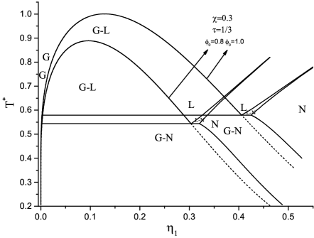
a
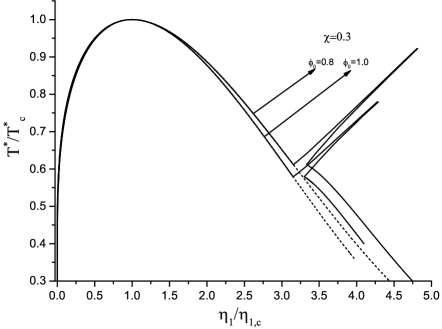
b

Fig. 1.: Temperature-density phase diagram calculated from the generalized van der Waals equation for hard spheres with isotropic and anisotropic attractive interactions ($\chi=0.3$) in random porous media with the porosity $\phi_{0}=0.8$ and $\tau=$ $=1/3$.  For the purpose of comparison, the phase diagram in the absence of a porous medium $\phi_{0}=1.0$ is also presented.  The dashed lines correspond to the case $\chi=0$.  On the top (case $a$), the phase diagram in the coordinates $T^{*}=kT/\epsilon_{0}$ and $\eta_{1}=\rho_{1}V_{1}$ is presented.  At the bottom (case $b$), the phase diagram is presented in the coordinates $T^{*}/T^{*}_{c}$ and $\eta_{1}/\eta_{1,c}$

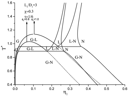
a

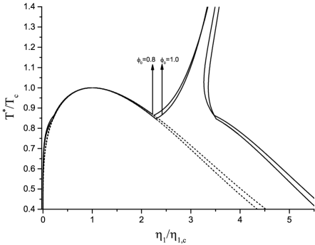
b

Fig. 2.: Temperature-density phase diagram calculated from the generalized van der Waals equation for hard spherocylinders with the anisotropy of sizes $L_{1}/D_{1}=3$ and with isotropic and anisotropic attractive interactions ($\chi=0.3$) in random porous media with the porosity $\phi_{0}=0.8$ and $\tau=1/6$.  For the purpose of comparison, the phase diagram in the absence of a porous medium $\phi_{0}=1.0$ is also presented.  The dashed lines correspond to the case $\chi=0$.  On the top (case $a$), the phase diagram in the coordinates $T^{*}=kT/\epsilon_{0}$ and $\eta_{1}=\rho_{1}V_{1}$ is presented.  At the bottom (case $b$), the phase diagram is presented in the coordinates $T^{*}/T^{*}_{c}$ and $\eta_{1}/\eta_{1,c}$

We start from the hard sphere model with attractive interactions in the form (36).  In this case, $L=0$, and $D=\sigma$ is the diameter of hard spheres.  The corresponding phase diagram is presented in Fig. 1.  In the region of small densities, we have the gas phase $G,$ which changes, as the density increases, to the liquid phase $L$ and, at higher densities, to the anisotropic nematic phase $N$.  The nematic phase appears due to the anisotropy of attractive interactions, and the bifurcation line of the nematic phase is proportional to $\frac{\rho_{1}\beta\chi}{\phi_{0}},$ according to (41). This means that the phase transition appears at higher densities and vice versa, as the temperature increases.  As the temperature decreases, the phase transition appears at lower densities.  At sufficiently low temperatures, the region of the gas-liquid transition converges to the tricritical gas-liquid-nematic $(G-L-N)$ point.  Below the tricritical point, only the gas-nematic $(GN)$ coexistence is seen.  At temperatures higher than the tricritical one, the anisotropic attractive interaction does not change the gas-liquid coexistence line in the van der Waals approximation.  But, for lower temperatures, the anisotropic attraction slightly widens the gas-liquid coexistence and leads to a strong widening for larger densities.  The presence of a porous medium shifts the phase diagram to the region of lower densities and lower temperature, as the porosity $\phi_{0}$ decreases.  In contrast to the usual gas-liquid phase transition [31], the law of corresponding states in the considered case is more or less valid in the region of small densities.  But, at higher densities, the coexistence curve becomes wider, as the porosity decreases.

The influence of the parameter $L_{1}/D_{1}$ responsible for the anisotropy of a molecular shape is presented in Figs. 2–4. Comparing Fig. 1 and Fig. 2, we can see that the non-sphericity of a molecular shape leads to a shift of the phase diagram to lower densities and higher temperatures.  The increase of the ratio $L_{1}/D_{1}$ leads to an increase of the critical temperature and a decrease of the critical density for the gas-liquid transition.  The tricritical temperature increases also, and the gas-liquid region is essentially narrower than in the case of spherical molecules.  Similarly as for $L_{1}/D_{1}=0$ (Fig. 1), the anisotropic phase appears in the case $L_{1}/D_{1}=3$ (Fig. 2) due to the anisotropy of attractive intermolecular interactions. However, the anisotropy of molecule shapes highly modifies the region of the coexistence of isotropic and nematic phases.  The liquid-nematic coexistence region becomes wider and is not very sensitive to the temperature.  Similarly as for $L_{1}/D_{1}=0$ below the tricritical temperature, the anisotropic attractive interaction does not change the gas-liquid coexistence line.  For lower temperatures, the coexistence region slightly widens at lower densities and widens significantly at higher densities.  We note that, at $\chi=0,$ the nematic phase does not appear.  In agreement with the data of computer simulations [32], the nematic phase in the fluid of hard spherocylinders appears at $L_{1}/D_{1}>3.7$.  For $L_{1}/D_{1}=3$ similarly as for $L_{1}/D_{1}=0,$ the decrease of the porosity $\phi_{0}$ shifts the phase diagram to lower densities and lower temperatures.  In contrast to the case $L_{1}/D_{1}=0$, the corresponding law in the case $L_{1}/D_{1}=3$ is more or less satisfied for all densities, including the region of the isotropic-nematic transition.

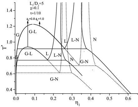
a

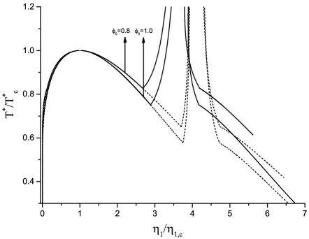
b

Fig. 3.: Temperature-density phase diagram calculated from the generalized van der Waals equation for hard spherocylinders with the anisotropy of sizes $L_{1}/D_{1}=5$ and with isotropic and anisotropic attractive interactions ($\chi=0.3$) in random porous media with the porosity $\phi_{0}=0.8$ and $\tau=0.1$. For the purpose of comparison, the phase diagram in the absence of a porous medium, $\phi_{0}=1.0,$ is also presented.  The dashed lines correspond to the case $\chi=0$.  On top (case $a$), the phase diagram in the coordinates $T^{*}=kT/\epsilon_{0}$ and $\eta_{1}=\rho_{1}V_{1}$ is presented.  At the bottom (case $b$), the phase diagram is presented in the coordinates $T^{*}/T^{*}_{c}$ and $\eta_{1}/\eta_{1,c}$

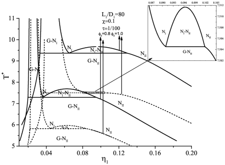
a

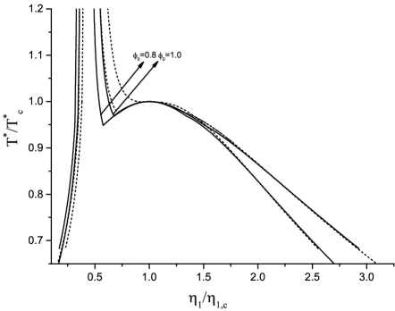
b

Fig. 4.: Temperature-density phase diagram calculated from the generalized van der Waals equation for hard spheres $L_{1}/D_{1}=80$ with isotropic and anisotropic attractive interactions ($\chi=0.3$) in random porous media with the porosity $\phi_{0}=0.8$ and $\tau=0.01$.  For the purpose of comparison, the phase diagram in the absence of a porous medium, $\phi_{0}=1.0,$ is also presented. The dashed lines correspond to the case $\chi=0$.  On top (case $a$), the phase diagram in the coordinates $T^{*}=kT/\epsilon_{0}$ and $\eta_{1}=\rho_{1}V_{1}$ is presented.  At the bottom (case $b$), the phase diagram is presented in the coordinates $T^{*}/T^{*}_{c}$ and $\eta_{1}/\eta_{1,c}$

The phase diagram for the case $L_{1}/D_{1}=5$ is presented in Fig. 3.  Such asymmetry of the shape of molecules is sufficient for the nematic ordering.  As we noted in [17], the anisotropic attractive interaction expands the region of orientational ordering.  The liquid-nematic region widens significantly if $\chi$ increases.  As a consequence, the gas-liquid transition disappears for a sufficiently large anisotropy, and only the isotropic-nematic transition takes place.  Such situation for $L_{1}/D_{1}=5$ is observed at $\chi=0.3$. Due to this fact, we put $\chi=0.1$ in Figs. 3 and 4.  As we can see from Fig. 3, similarly to Figs. 1 and 2, the gas-liquid coexistence line below the tricritical temperature does not depend on the anisotropic attractive interaction. The anisotropic attractive interaction leads to an increase of the tricritical temperature and a decrease of the tricritical density. As a result, the gas-liquid region is narrower, while the liquid-nematic region covers a wide range of densities.  The presence of a porous medium shifts the phase diagram to lower densities and lower temperatures.  The corresponding law is satisfied rather well.  In the region of the anisotropic transition, the corresponding law is satisfied separately for $\chi=0$ and for $\chi=0.1$.

Finally, we consider Fig. 4, where the phase diagram for $L_{1}/D_{1}=80$ is presented.  As we noted in [17], the transition into the nematic phase shifts in this case at $\chi=0$ to the region of small densities.  As a consequence, the gas-liquid transition appears in the nematic region.  In accordance with the classification in [33], the gas phase in the nematic region is marked as $N_{I},$ and the liquid phase in the nematic region is marked as $N_{II}$.  In contrast to the previous figures, in the case considered in Fig. 4, the influence of an anisotropic attractive interaction is of importance for the entire phase diagram.  The anisotropic attractive interaction does not change significantly the critical density of the gas-liquid transition, but it changes strongly the value of critical temperature.  In contrast to the case $L_{1}/D_{1}=5,$ the anisotropic attractive interaction in the considered case $L_{1}/D_{1}=80$ leads to a strong increase of the tricritical temperature and to the expansion of the gas-liquid coexistence.  The region of coexistence of the isotropic and nematic phases is also expanded and shifts to lower densities.  In the presence of a porous medium, the phase diagram is shifted to lower densities and lower temperatures, as the porosity $\phi_{0}$ decreases.  The corresponding law is satisfied quite well for the isotropic phase independently of the value of $\chi$.  However, the values of $\chi$ and porosity $\phi_{0}$ have a strong influence on the phase diagram in the anisotropic region.  At the critical point, the corresponding law is satisfied, but, for higher densities, the behavior of the phase diagram depends significantly on the value of porosity $\phi_{0}$.

5 Conclusion

In this paper, we have presented the generalized van der Waals equation for anisotropic molecular fluids in porous media.  This generalization is based on analytical expressions for the equation of state and the chemical potential of a hard spherocylinder fluid in a random porous medium obtained in the framework of the scaled particle theory.  The second term of the generalized van der Waals equation is the mean value of attractive intermolecular interactions.  By minimizing the free energy of the fluid, we have obtained a nonlinear integral equation for the singlet distribution function, which describes the orientational ordering in the system. This ordering is connected with the non-sphericity of molecular shapes and the anisotropy of intermolecular attractive interactions.

The investigations based on the generalized van der Waals equation demonstrate a wide variety of gas-liquid-nematic phase behaviors in molecular systems depending on the anisotropy of a shape of molecules, anisotropy of attractive interparticle interactions, and porosity of a porous medium.  Here, we have focused our attention on the influence of the anisotropy of attractive interactions, which is the main reason for the orientational ordering in quasispherical molecules.  It is shown that the anisotropy of molecular shapes leads to a shift of the critical point of the gas-liquid transition to lower densities and higher temperatures and to an increase in the tricritical temperature.  The anisotropy of molecular shapes also expands significantly the region of coexistence of the isotropic and nematic phases.  It is shown that, for a larger anisotropy, the nematic phase can appear due to the anisotropy of molecular shapes. In this case, the anisotropy of attractive intermolecular interactions expands significantly the region of coexistence between the isotropic and nematic phases and shifts it to the region of lower densities and higher temperatures.  Finally, at a sufficiently large anisotropy of molecular shapes, the transition into the nematic phase takes place at very low densities.  As a result, the gas-liquid transition takes place in the nematic region. In all the considered cases, the decrease of the porosity of a porous medium shifts the phase diagram to the region of lower temperatures and lower densities.

The authors express their gratitude to Taras Patsahan and Ivan Kravtsiv for useful discussions and important suggestions during the preparation of this paper.

М.Ф. Головко, В.I. Шмотолоха
УЗАГАЛЬНЕННЯ РIВНЯННЯ
ВАН-ДЕР-ВААЛЬСА НА АНIЗОТРОПНI
РIДИНИ В ПОРИСТИХ СЕРЕДОВИЩАХ
Р е з ю м е
Представлене узагальнене рiвняння Ван-дер-Ваальса на анiзотропнi рiдини в пористих середовищах складається з двох доданкiв. Перший з них базується на рiвняннi стану твердих сфероцилiндрiв у випадковому пористому середовищi, отриманий в рамках методу узагальнення масштабної частинки. Другий доданок виражається через середнє значення потенцiалу притягальної мiжмолекулярної взаємодiї. На основi отриманого рiвняння проведено дослiдження фазової поведiнки газ–рiдина–нематик молекулярних систем у залежностi вiд анiзотропiї форми молекул, анiзотропiї притягальної взаємодiї та пористостi пористого середовища. Показано, що анiзотропна фаза формується як за рахунок анiзотропної притягальної взаємодiї, так i за рахунок анiзотропiї форми молекул. Анiзотропiя форми молекул приводить до зсуву фазової дiаграми в область менших густин та вищих температур, а анiзотропiя притягальної взаємодiї значно розширює область спiвiснування iзотропної та нематичної фаз i також зсовує її в область нижчих густин i вищих температур. Показано, що при достатньо великiй асиметрiї форми молекул фазовий перехiд рiдина–газ знаходиться повнiстю в областi нематичної фази. У всiх випадках, що розглядаються, пониження пористостi пористого середовища зсовує фазову дiаграму в область нижчих густин i температур.

References

- [1] L.A. Bulavin, Critical Properties of Liquids (АСМI, Kyiv, 2002) (in Ukrainian).
- [2] L.A. Bulavin, G.N. Verbinskaya, and I.N. Vishnevskii, Quasielastic Neutron Scattering in Liquids (АСМI, Kyiv, 2004) (in Ukrainian).
- [3] L.A. Bulavin, T.V. Karmazina, V.V. Klepko, and V.I. Slisenko, Neutron Spectroscopy of Condensed Matter (Akademperiodyka, Kyiv, 2005) (in Ukrainian).
- [4] I.I. Adamenko and L.A. Bulavin, Physics of Liquids and Liquid Systems (АСМI, Kyiv, 2006) (in Ukrainian).
- [5] L.A. Bulavin, Neutron Diagnostics of Liquid State of Matter (Chornobyl, 2012) (in Ukrainian).
- [6] J.D. van der Waals, in Studies in Statistical Mechanics, 14, ed. by J.S. Rowlinson, (North-Holland, Amsterdam, 1988).
- [7] M. Kac, G.E. Uhlenbeck, and P.C. Hammer, J. Math. Phys. 4, 216 (1963).
- [8] J.L. Lebowitz and O. Penrose, J. Math. Phys. 7, 98 (1966).
- [9] I.R. Yukhnovsky and M.F. Holovko, Statistical theory of Classical Equilibrium Systems (Naukova Dumka, Kyiv, 1980) (in Russian).
- [10] L. Tonks, Phys. Rev. 50, 955 (1936).
- [11] N.F. Carnahan and K.E. Starling, J. Chem. Phys. 51, 635 (1969).
- [12] W.G. Madden and E.D. Glandt, J. Stat. Phys. 51, 537 (1988).
- [13] H. Reiss, H.L. Frisch, and J.L. Lebowitz, J. Chem. Phys. 31, 369 (1959).
- [14] H. Reiss, H.L. Frisch, E. Helfand, and J.L. Lebowitz, J. Chem. Phys. 32, 119 (1960).
- [15] T. Patsahan, M. Holovko, and W. Dong, J. Chem. Phys. 134, 074503 (2011).
- [16] M. Holovko, T. Patsahan, and W. Dong, Pure and Appl. Chem. 85, 115 (2013).
- [17] M. Holovko, V. Shmotolokha, and T. Patsahan, in Springer Proceedings in Physics, eds. L. Bulavin, N. Lebovka (Springer, Berlin, 2015), vol. 171.
- [18] M. Holovko, V. Shmotolokha, and T. Patsahan. J. Mol. Liq. 189, 30 (2014).
- [19] L. Onsager, Ann. N.Y. Acad. Sci. 51, 627 (1949).
- [20] G.J. Vroege, and H.N.W. Lekkerkerker, Rep. Progr. Phys. 55, 1241 (1992).
- [21] M. Holovko and W. Dong, J. Phys. Chem. B 113, 6360 (2009).
- [22] M.A. Cotter and D.E. Martire, J. Chem. Phys. 52, 1909 (1970).
- [23] M.A. Cotter, Phys. Rev. A 10, 625 (1974).
- [24] C.G. Gray and K.E. Gubbins, Theory of Molecular Fluids (Clarendon Press, Oxford, 1984).
- [25] M. Holovko, T. Patsahan, and W. Dong, Condens. Matter Phys. 15, 23607 (2012).
- [26] J. Herzfeld, A.E. Berger, and J.W. Wingate, Macromolecules 17, 1718 (1984).
- [27] R.F. Kayser, jr., and H.J. Raveche, Phys. Rev. A 17, 2067 (1978).
- [28] M. Schmidt and M. Dijkstra, J. Chem. Phys. 121, 12067 (2004).
- [29] W. Maier and A. Saupe, Z. Naturforsch, 14a, 882 (1959).
- [30] M. Franco-Melgar, A.J. Haslam, and G. Jackson, Mol. Phys. 107, 2329 (2009).
- [31] M. Holovko, T. Patsahan, and V. Shmotolokha, Cond. Matter Phys. 18, No. 1, 13607 (2015).
- [32] P. Bolhuis and D. Frenkel. J. Chem. Phys. 106, 666 (1997).
-
[33]
S. Varga, D.C. Williamson, and I.Szalai,
Mol. Phys. 96, 1695 (1999).
Received 12.05.15