Strong-coupling phases of 3D Dirac and Weyl semimetals. A renormalization group approach.

Abstract

We investigate the strong-coupling phases that may arise in 3D Dirac and Weyl semimetals under the effect of the long-range Coulomb interaction, considering the many-body theory of these electron systems as a variant of the conventional fully relativistic Quantum Electrodynamics (QED). For this purpose, we apply two different nonperturbative approaches, consisting in the sum of ladder diagrams and taking the limit of a large number $N$ of fermion flavors. We benefit from the renormalizability that the theory shows in both cases to compute the anomalous scaling dimensions of different operators exclusively in terms of the renormalized coupling constant, allowing us to determine the precise location of the singularities signaling the onset of the strong-coupling phases. We show then that the QED of 3D Dirac semimetals has two competing effects at strong coupling. One of them is the tendency to chiral symmetry breaking and dynamical mass generation, which are analogous to the same phenomena arising in the conventional QED at strong coupling. This trend is however outweighed by the strong suppression of electron quasiparticles that takes place at large $N$, leading to a different type of critical point at sufficiently large interaction strength, shared also by the 3D Weyl semimetals. Overall, the phase diagram of the 3D Dirac semimetals turns out to be richer than that of their 2D counterparts, displaying a transition to a phase with non-Fermi liquid behavior which may be observed in materials hosting a sufficiently large number of Dirac or Weyl points.

1 Introduction

In recent years, condensed matter physics has witnessed several remarkable discoveries that, starting from graphenenovo , have shown the existence of electron systems where the quasiparticles have linear dispersion about degenerate points at the intersection between valence and conduction bands. This has led to introduce the class of so-called Dirac semimetals, in which the low-energy excitations can be described in terms of a number of Dirac spinors. Thus, there is already clear evidence that materials like Na₃Bi or Cd₃As₂ have Dirac points in their electronic dispersionliu ; neu ; bor , providing in that respect a 3D electronic analogue of graphene. More recently, there have been claims that materials like TaAs or the pyrochlore iridates should be examples of 3D Weyl semimetalstaas1 ; taas2 , characterized by having Weyl points hosting each of them fermions with a given chirality.

Since the appearance of graphene, the possibility that the quasiparticles of a condensed matter system may behave as Dirac fermions has been very appealing, as the particular geometrical features of these mathematical objects have shown to be indeed at the origin of several unconventional effects. The Klein paradoxkats and the difficulty that such quasiparticles have to undergo backscatteringando are a direct consequence of the additional pseudospin degree of freedom inherent to Dirac fermions. The topological insulators and their peculiar surface states can be taken also as an illustration of the fruitful interplay arising between the symmetry properties of Dirac fermions and the topology of the spacekane ; qi .

Another important feature of known Dirac semimetals is that they need to be modeled as interacting electron systems which are naturally placed in the strong-coupling regime. This is so as the long-range Coulomb repulsion becomes the dominant interaction, while the Fermi velocity of the electrons takes values which are at least two orders of magnitude below the speed of light. Thus, the equivalent of the fine structure constant in the electron system can be more than one hundred times larger than its counterpart in the conventional fully relativistic Quantum Electrodynamics (QED). This leads to expect relevant many-body effects as, for instance, the imperfect screening of impurities with sufficiently large charge on top of graphenenil ; fog ; shy ; ter . Another important property is the scale dependence of physical observables, like that predicted theoretically for the Fermi velocity in 2D Dirac semimetalsnp2 ; prbr and measured recently in suspended graphene samples at very low doping levelsexp2 . We may think therefore of the Dirac semimetals as an ideal playground to observe scaling phenomena that would be otherwise confined to the investigation of field theories in particle physics.

In any event, a proper account of the scaling effects must rely on the renormalizability of the many-body theory. The formulation of the interacting theory of Dirac semimetals requires the introduction of a high-energy cutoff in the electronic spectrum, which can be set to a rather arbitrary level. In order to ensure the predictability of the theory, it becomes therefore crucial that all the dependences on the high-energy cutoff can be absorbed into the redefinition of a finite number of parameters. In the case of Dirac semimetals, such a renormalizability cannot be taken for granted, as the many-body theory does not enjoy the full covariance which enforces that property in typical relativistic field theories. Nevertheless, the investigation of the 2D Dirac semimetals has already provided evidence that the interacting field theory in these electron systems is renormalizablejhep . This condition has allowed for instance to compute very high order contributions to the renormalization of relevant order parameters, leading to an estimate of the critical coupling for chiral symmetry breaking that agrees with the value obtained with a quite different nonperturbative method like the resolution of the gap equationgama .

The aim of this paper is to investigate the strong-coupling phases that may arise in 3D Dirac and Weyl semimetals under the effect of the long-range Coulomb interaction. In this respect, the many-body theory of these electron systems can be viewed as a variant of conventional QED. As already pointed out, a main difference with this theory lies in that the Fermi velocity of the electrons does not coincide with the speed of light, which makes that quasiparticle parameter susceptible of being renormalized and therefore dependent on the energy scale. In three spatial dimensions, the electron charge needs also to be redefined to account for cutoff dependences of the bare theory, which renders the question of the renormalizability even more interesting in the present context.

In this paper we will apply two different nonperturbative approximations to the QED of 3D Dirac and Weyl semimetals, namely the ladder approach and the large-$N$ approximation ($N$ being the number of different fermion flavors), which can be viewed as complementary computational methods. In both cases, we will see that the field theory appears to be renormalizable, making possible to absorb all the dependences on the high-energy cutoff into a finite number of renormalization factors given only in terms of the renormalized coupling.

We will show that the QED of 3D Dirac semimetals has two competing effects at strong coupling. One of them is the tendency to chiral symmetry breaking and dynamical mass generation, which are analogous to the same phenomena arising in the conventional QED at strong couplingmas ; fom ; fuk ; mir ; gus2 ; kon ; atk ; min . This trend is however outweighed by the strong suppression of electron quasiparticles that takes place at large $N$, leading then to a different type of critical point at sufficiently large interaction strengthrc , shared also by the 3D Weyl semimetals. We will see that the nonperturbative approaches applied in the paper afford a precise characterization of the respective critical behaviors in terms of the anomalous dimensions of relevant operators. At the end, the phase diagram of the 3D Dirac semimetals turns out to be richer than that of their 2D counterparts, displaying a transition to a phase with non-Fermi liquid behavior (genuine also of the 3D Weyl semimetals) which may be observed in materials hosting a sufficiently large number of Dirac or Weyl points.

2 Field theory of 3D Dirac and Weyl semimetals

Our starting point is the field theory describing the 3D fermions with linear dependence of the energy $\varepsilon$ on momentum ${\bf p}$, $\varepsilon({\bf p})=v_{F}|{\bf p}|$, and interacting through the scalar part $\phi$ of the electromagnetic potential. The fermion modes can be encoded into a number $N$ of spinor fields $\psi_{i}$, $i=1,\ldots N$, where the index $i$ represents in general the way in which the modes are distributed into different Dirac or Weyl points in momentum space. For convenience, we will choose to pair the fermion chiralities into four-component spinors, extending the notation to think of each $\psi_{i}$ field as being made of two different chiralities from a given Dirac point, or from two different Weyl points in the case of a Weyl semimetal. The hamiltonian can be written then as

$$H=-iv_{F}\int d^{3}r\;\overline{\psi}_{i}({\bf r})\boldsymbol{\gamma}\cdot\boldsymbol{\partial}\psi_{i}({\bf r})+e_{0}\int d^{3}r\;\overline{\psi}_{i}({\bf r})\gamma_{0}\psi_{i}({\bf r})\>\phi({\bf r})$$ (1)

where $\overline{\psi}_{i}=\psi_{i}^{\dagger}\gamma_{0}$ and $\{\gamma_{\sigma}\}$ is a collection of four-dimensional matrices such that $\{\gamma_{\mu},\gamma_{\nu}\}=2\>{\rm diag}(1,-1,-1,-1)$.

In order to complete the field theory, we have to provide the propagator of the scalar field $\phi$, for which we take the Lorentz gauge in the dynamics of the full electromagnetic potential. Thus, we get from the original relativistic theory

$$\langle T\phi({\bf r},t)\phi({\bf r}^{\prime},t^{\prime})\rangle=-i\int\frac{d^{3}q}{(2\pi)^{3}}\int\frac{d\omega}{2\pi}e^{i{\bf q}\cdot({\bf r}-{\bf r}^{\prime})}e^{-i\omega(t-t^{\prime})}\frac{1}{{\bf q}^{2}-\omega^{2}/c^{2}-i\eta}$$ (2)

We are interested in systems where the Fermi velocity $v_{F}$ is much smaller than the speed of light $c$, which makes possible to adopt a simpler description taking the limit $c\rightarrow\infty$. This justifies that we can neglect magnetic interactions between our nonrelativistic fermions, and that we can just deal with the zero-frequency limit of (2). Thus, the free propagator for the scalar potential will be taken in what follows as

$$D_{0}({\bf q})=\frac{1}{{\bf q}^{2}}$$ (3)

A remarkable property is that the hamiltonian (1) together with the interaction mediated by (3) define an interacting field theory that is scale invariant at the classical level. That is, under a change in the scale of the space and time variables

$$t\rightarrow st\;\;\;\;,\;\;\;\;{\bf r}\rightarrow s{\bf r}$$ (4)

the fields can be taken to transform accordingly as

$$\phi({\bf r})\rightarrow\frac{1}{s}\phi({\bf r})\;\;\;\;,\;\;\;\;\psi({\bf r})\rightarrow\frac{1}{s^{3/2}}\psi({\bf r})$$ (5)

This gives rise to a homogeneous scaling of the hamiltonian (1), consistent with the transformation of an energy variable.

Such a scale invariance has important consequences, since it makes possible to give meaning to the divergences that the field theory develops at high energies. The computation of the quantum corrections requires indeed the introduction of a high-energy cutoff that spoils the classical scale invariance. However, provided the field theory is renormalizable, the singular dependences on the cutoff can be still absorbed into a finite number of renormalization factors redefining the parameters of the theory. Writing the action $S$ corresponding to the hamiltonian (1), we may start with a formulation introducing suitable renormalization factors $Z_{\psi},Z_{v},Z_{e}$ and $Z_{\phi}$:

$$S=\int dt\>d^{3}r\;Z_{\psi}\>\overline{\psi}_{i}({\bf r})(i\gamma_{0}\partial_{t}+iZ_{v}v_{R}\boldsymbol{\gamma}\cdot\boldsymbol{\partial})\psi_{i}({\bf r})-Z_{e}e\int dt\>d^{3}r\;Z_{\psi}\>\overline{\psi}_{i}({\bf r})\gamma_{0}\psi_{i}({\bf r})\>Z_{\phi}\phi({\bf r})$$ (6)

The gauge invariance of the model implies that $Z_{e}Z_{\phi}=1$. The point is that, if the field theory is well-behaved, one has to be able to render all the physical observables cutoff-independent, when written in terms of the renormalized parameters $v_{R}$ and $e$.

The first example of the need to implement a high-energy cutoff can be taken from the computation of the electron self-energy. The first perturbative contribution is given by the first rainbow diagram at the right-hand-side in Fig. 1, which corresponds to the expression

$$i\Sigma_{1}({\bf k})=-e_{0}^{2}\int\frac{d^{3}p}{(2\pi)^{3}}\int\frac{d\omega_{p}}{2\pi}\gamma_{0}\frac{-\gamma_{0}\omega_{p}+v_{F}\boldsymbol{\gamma}\cdot{\bf p}}{-\omega_{p}^{2}+v_{F}^{2}{\bf p}^{2}-i\eta}\gamma_{0}\frac{1}{({\bf k}-{\bf p})^{2}}$$ (7)

This contribution to the electron self-energy does not depend on frequency, but shows a divergent behavior at the upper end of the momentum integration, pointing at the renormalization of the Fermi velocity $v_{F}$. In what follows, instead of dealing with a cutoff in momentum space, we will prefer to use a regularization method that is able to preserve the gauge invariance of the model. For this purpose, we will adopt the analytic continuation of the momentum integrals to dimension $D=3-\epsilon$, which will convert all the high-energy divergences into poles in the $\epsilon$ parameterram .

In the dimensional regularization method, the bare charge $e_{0}$ must get dimensions through an auxiliary momentum scale $\mu$, being related to the physical dimensionless charge $e$ by

$$e_{0}=\mu^{\epsilon/2}e$$ (8)

The computation of the first-order contribution to the self-energy (7) gives then

$$\Sigma_{1}({\bf k}) = \frac{e^{2}}{2}\mu^{\epsilon}\int\frac{d^{D}p}{(2\pi)^{D}}\boldsymbol{\gamma}\cdot{\bf p}\frac{1}{|{\bf p}|}\frac{1}{({\bf k}-{\bf p})^{2}}$$ (9)

$$= \frac{e^{2}}{4}\mu^{\epsilon}\int\frac{d^{D}p}{(2\pi)^{D}}\boldsymbol{\gamma}\cdot{\bf p}\int_{0}^{1}dx\frac{(1-x)^{-1/2}}{[({\bf k}-{\bf p})^{2}x+{\bf p}^{2}(1-x)]^{3/2}}$$

$$= \frac{e^{2}}{4}\boldsymbol{\gamma}\cdot{\bf k}\>\mu^{\epsilon}\int\frac{d^{D}p}{(2\pi)^{D}}\int_{0}^{1}dx\frac{x(1-x)^{-1/2}}{[{\bf p}^{2}+{\bf k}^{2}x(1-x)]^{3/2}}$$

$$= \frac{e^{2}}{2\sqrt{\pi}}\boldsymbol{\gamma}\cdot{\bf k}\frac{\Gamma\left(\tfrac{3}{2}-\tfrac{D}{2}\right)}{(4\pi)^{D/2}}\mu^{\epsilon}\int_{0}^{1}dx\frac{x(1-x)^{-1/2}}{[{\bf k}^{2}x(1-x)]^{3/2-D/2}}$$

$$= \frac{e^{2}}{(4\pi)^{2-\epsilon/2}}\boldsymbol{\gamma}\cdot{\bf k}\frac{\mu^{\epsilon}}{|{\bf k}|^{\epsilon}}\frac{\Gamma\left(\tfrac{1}{2}\epsilon\right)\Gamma\left(2-\tfrac{\epsilon}{2}\right)\Gamma\left(\tfrac{1}{2}-\tfrac{\epsilon}{2}\right)}{\Gamma\left(\tfrac{5}{2}-\epsilon\right)}$$

The expression (9) shows the development of a $1/\epsilon$ pole as $\epsilon\rightarrow 0$. This divergence can be indeed absorbed into a renormalization of the Fermi velocity $v_{F}$, as the full fermion propagator $G({\bf k},\omega)$ is related to the self-energy $\Sigma({\bf k},\omega)$ by

$$G({\bf k},\omega)^{-1}=Z_{\psi}(\gamma_{0}\omega-Z_{v}v_{R}\boldsymbol{\gamma}\cdot{\bf k})-Z_{\psi}\Sigma({\bf k},\omega)$$ (10)

Thus, to first order in $e^{2}$, the fermion propagator can be made finite in the limit $\epsilon\rightarrow 0$ by taking

$$Z_{v}=1-\frac{e^{2}}{6\pi^{2}v_{R}}\frac{1}{\epsilon}$$ (11)

This renormalization of the fermion propagator already gives an idea of the effective dependence of the Fermi velocity on the energy scale. The bare Fermi velocity $Z_{v}v_{R}$ cannot depend on the momentum scale $\mu$, since the original theory does not know about that auxiliary scale. We have therefore

$$\mu\frac{\partial}{\partial\mu}(Z_{v}v_{R})=0$$ (12)

For the same reason, the bare coupling $e_{0}$ cannot depend on $\mu$, which leads to the equation

$$\mu\frac{\partial}{\partial\mu}e=-\frac{\epsilon}{2}e$$ (13)

Combining (12) and (13), we arrive at the scaling equation

$$\mu\frac{\partial}{\partial\mu}v_{R}=-\frac{1}{6\pi^{2}}e^{2}$$ (14)

This is the expression of the growth of the renormalized Fermi velocity $v_{R}$ in the low-energy limit, approached here as $\mu\rightarrow 0$. This scaling, which parallels the behavior of the Fermi velocity in 2D Dirac semimetals, is the main physical property deriving from the lowest-order renormalization of the 3D Dirac and Weyl semimetalsros .

To close this section, we comment that the result (9) for the electron self-energy has actually a wider range of validity, beyond the lowest-order approximation in which it has been obtained. This can be seen by exploiting a feature that is also shared with the 2D Dirac semimetals in the so-called ladder approximation, that is when corrections to the interaction vertex and the interaction propagator are neglected in the electron self-energyjhep . Then we remain with the sum of diagrams encoded in the self-consistent equation represented in Fig. 1. The electron self-energy in this approximation, $\Sigma_{\rm ladder}({\bf k})$, must have the form

$$\Sigma_{\rm ladder}({\bf k})=f({\bf k})\>\boldsymbol{\gamma}\cdot{\bf k}$$ (15)

and therefore it is bound to satisfy the equation

$$i\Sigma_{\rm ladder}({\bf k})=i\Sigma_{1}({\bf k})+e_{0}^{2}\int\frac{d^{D}p}{(2\pi)^{D}}\int\frac{d\omega_{p}}{2\pi}\Sigma_{\rm ladder}({\bf p})\frac{\omega_{p}^{2}+v_{F}^{2}{\bf p}^{2}}{(-\omega_{p}^{2}+v_{F}^{2}{\bf p}^{2}-i\eta)^{2}}\frac{1}{({\bf k}-{\bf p})^{2}}$$ (16)

It is now easy to see that the second term at the right-hand-side of (16) identically vanishes. By performing a Wick rotation $\omega_{p}=i\overline{\omega}_{p}$, we get

$$\int\frac{d\omega_{p}}{2\pi}\frac{\omega_{p}^{2}+v_{F}^{2}{\bf p}^{2}}{(-\omega_{p}^{2}+v_{F}^{2}{\bf p}^{2}-i\eta)^{2}}=i\int\frac{d\overline{\omega}_{p}}{2\pi}\frac{-\overline{\omega}_{p}^{2}+v_{F}^{2}{\bf p}^{2}}{(\overline{\omega}_{p}^{2}+v_{F}^{2}{\bf p}^{2})^{2}}=0$$ (17)

showing that

$$\Sigma_{\rm ladder}({\bf k})=\Sigma_{1}({\bf k})$$ (18)

Figure 1: Diagrammatic representation of the ladder approximation for the electron self-energy.

The result (18) has important consequences for the ladder approximation, since it implies that the low-energy scaling of the Fermi velocity is again the main physical effect derived from the electron self-energy, limiting the possible electronic instabilities that can arise in that nonperturbative approach.

3 3D Dirac semimetals in ladder approximation

The iterative sequence of interactions, illustrated in Fig. 1 for the electron self-energy, defines a partial sum of perturbation theory which can be also applied to analyze the renormalization of composite operators. This provides a suitable approach to investigate possible instabilities of the electron system, since some of those operators correspond to order parameters characterizing the breakdown of respective symmetries of the field theory. Once the renormalization program is accomplished, the singularities found in the correlators of the composite operators may signal the condensation of a given order parameter, pointing at the onset of a new phase of the electron system.

The most relevant composite operators are made of bilinears of the fermion fields, having associated vertex functions that can be used to measure different susceptibilities of the electron system. At this point, the discussion is confined to the 3D Dirac semimetals (excluding the case of Weyl semimetals), for which we can write different composite operators in terms of four-component spinors about the same Dirac point in momentum space. We pay attention in particular to those operators corresponding to the charge, the current, and the fermion mass, given by

$$\rho_{0}({\bf r}) = \overline{\psi}_{i}({\bf r})\gamma_{0}\psi_{i}({\bf r})$$ (19)

$$\boldsymbol{\rho}_{c}({\bf r}) = \overline{\psi}_{i}({\bf r})\>\boldsymbol{\gamma}\>\psi_{i}({\bf r})$$ (20)

$$\rho_{m}({\bf r}) = \overline{\psi}_{i}({\bf r})\psi_{i}({\bf r})$$ (21)

The respective one-particle-irreducible (1PI) vertices are

$$\Gamma_{0}({\bf q},\omega_{q};{\bf k},\omega_{k}) = \langle\rho_{0}({\bf q},\omega_{q})\psi_{i}({\bf k}+{\bf q},\omega_{k}+\omega_{q})\overline{\psi}_{i}({\bf k},\omega_{k})\rangle_{\rm 1PI}$$ (22)

$$\boldsymbol{\Gamma}_{c}({\bf q},\omega_{q};{\bf k},\omega_{k}) = \langle\boldsymbol{\rho}_{c}({\bf q},\omega_{q})\psi_{i}({\bf k}+{\bf q},\omega_{k}+\omega_{q})\overline{\psi}_{i}({\bf k},\omega_{k})\rangle_{\rm 1PI}$$ (23)

$$\Gamma_{m}({\bf q},\omega_{q};{\bf k},\omega_{k}) = \langle\rho_{m}({\bf q},\omega_{q})\psi_{i}({\bf k}+{\bf q},\omega_{k}+\omega_{q})\overline{\psi}_{i}({\bf k},\omega_{k})\rangle_{\rm 1PI}$$ (24)

The point is that, assuming the renormalizability of the field theory, there must exist a multiplicative renormalization of the vertices

$$\Gamma_{0,{\rm ren}} = Z_{0}\Gamma_{0}$$ (25)

$$\boldsymbol{\Gamma}_{c,{\rm ren}} = Z_{c}\boldsymbol{\Gamma}_{c}$$ (26)

$$\Gamma_{m,{\rm ren}} = Z_{m}\Gamma_{m}$$ (27)

that renders $\Gamma_{0,{\rm ren}},\boldsymbol{\Gamma}_{c,{\rm ren}}$ and $\Gamma_{m,{\rm ren}}$ independent of the high-energy cutoff. We check next that property of the field theory, dealing with the same iteration of the interaction applied before to the electron self-energy. In the present context, this defines the ladder approximation as given by the self-consistent diagrammatic equation represented for a generic vertex in Fig. 2.

Figure 2: Self-consistent diagrammatic equation for a generic vertex $\Gamma_{i}$ in the ladder approximation.

We first observe that the renormalization of $\Gamma_{0}$ must be dictated by the gauge invariance of the model, since the composite operator $\rho_{0}({\bf r})$ already appears in the action (6). This implies the result

$$Z_{0}=Z_{\psi}$$ (28)

meaning that, according to the previous analysis of the self-energy, it must be $Z_{0}=1$ in the ladder approximation. Moreover, the composite operator $\boldsymbol{\rho}_{c}$ may be introduced in the action multiplying it by the vector potential, showing that its renormalization can be related by gauge invariance to that of the kinetic term in (1). We conclude therefore that

$$Z_{c}=Z_{\psi}Z_{v}$$ (29)

which, in the ladder approximation, leads to $Z_{c}=Z_{v}$.

The results (28) and (29) can be also obtained more formally from the Ward idendities that reflect the gauge invariance of the model at the quantum level. They lead in particular to the equations

$$\frac{\partial}{\partial\omega}\left(\gamma_{0}\omega-\Sigma({\bf k},\omega)\right) = \Gamma_{0}({\bf 0},0;{\bf k},\omega)$$ (30)

$$\frac{1}{v_{F}}\frac{\partial}{\partial{\bf k}}\left(v_{F}\boldsymbol{\gamma}\cdot{\bf k}+\Sigma({\bf k},\omega)\right) = \boldsymbol{\Gamma}_{c}({\bf 0},0;{\bf k},\omega)$$ (31)

These identities were used in Ref. jhep to check the suitability of the dimensional regularization method to preserve the gauge invariance of the field theory of 2D Dirac semimetals. It was shown there that, if the the electron self-energy is computed with the set of diagrams encoded in the equation of Fig. 1, then the Ward identities are satisfied when one takes for the vertex the series of ladder diagrams, but dressed with the lowest-order electron self-energy correction. With this scope of the nonperturbative approach, it can be also shown by direct renormalization of $\boldsymbol{\Gamma}_{c}$ that $Z_{c}$ becomes as simple as the expression given by (11), which arises then from a remarkable cancellation of different contributions in the computation of the vertex.

We conclude that the charge operator is not renormalized, while the current operator requires a multiplicative redefinition by the simple factor (11) in the ladder approximation. The absence of a singularity for any value of the coupling constant excludes the possibility of having an instability related to the condensation of the charge or the current in the electron system. We turn now to the case of the mass vertex (24), whose renormalization is not dictated by the previous analysis of the electron self-energy.

3.1 Mass vertex and dynamical mass generation

Our starting point for the analysis of the mass vertex in the ladder approximation is the self-consistent equation represented in Fig. 2. We are going to be mainly interested in the renormalization of $\Gamma_{m}$ and, for that purpose, it is enough to consider the limit of momentum transfer ${\bf q}\rightarrow 0$ and $\omega_{q}\rightarrow 0$. The vertex must satisfy then the equation

$$\Gamma_{m}({\bf 0},0;{\bf k},\omega_{k})=$$ (32)

$$1+ie^{2}_{0}\int\frac{d^{D}p}{(2\pi)^{D}}\frac{d\omega_{p}}{2\pi}\gamma_{0}\frac{-\gamma_{0}\omega_{p}+v_{F}\boldsymbol{\gamma}\cdot{\bf p}}{-\omega_{p}^{2}+v_{F}^{2}{\bf p}^{2}-i\eta}\Gamma_{m}({\bf 0},0;{\bf p},\omega_{p})\frac{-\gamma_{0}\omega_{p}+v_{F}\boldsymbol{\gamma}\cdot{\bf p}}{-\omega_{p}^{2}+v_{F}^{2}{\bf p}^{2}-i\eta}\gamma_{0}\frac{1}{({\bf k}-{\bf p})^{2}}\;\;\;\;\;\;\;\;\;\;$$

The resolution of (32) implies that $\Gamma_{m}$ has to be proportional to the identity matrix. Moreover, it turns out to be a function independent of the frequency $\omega_{k}$ in this approximation. After a little algebra, we arrive then at the simplified equation

$$\Gamma_{m}({\bf 0},0;{\bf k},\omega_{k})=1+\frac{e_{0}^{2}}{2}\int\frac{d^{D}p}{(2\pi)^{D}}\Gamma_{m}({\bf 0},0;{\bf p},\omega_{k})\frac{1}{v_{F}|{\bf p}|}\frac{1}{({\bf k}-{\bf p})^{2}}$$ (33)

Eq. (33) can be solved by means of an iterative procedure, expressing the vertex as a power series in the effective coupling $\lambda_{0}=e_{0}^{2}/4\pi v_{F}$,

$$\Gamma_{m}({\bf 0},0;{\bf k},\omega_{k})=1+\sum_{n=1}^{\infty}\lambda_{0}^{n}\>\Gamma_{m}^{(n)}({\bf k})$$ (34)

Assuming that the term $\Gamma_{m}^{(n)}({\bf k})$ is proportional to $1/|{\bf k}|^{n\epsilon}$, the next order can be computed consistently from (33), taking into account that

$$\Gamma_{m}^{(n+1)}({\bf k}) \sim \frac{1}{2}\int\frac{d^{D}p}{(2\pi)^{D}}\frac{1}{|{\bf p}|^{1+n\epsilon}}\frac{1}{({\bf k}-{\bf p})^{2}}$$ (35)

$$= \frac{(4\pi)^{\epsilon/2}}{16\pi^{3/2}}\frac{\Gamma\left(\tfrac{n+1}{2}\epsilon\right)\Gamma\left(1-\tfrac{(n+1)\epsilon}{2}\right)\Gamma\left(\tfrac{1-\epsilon}{2}\right)}{\Gamma\left(\tfrac{1+n\epsilon}{2}\right)\Gamma\left(\tfrac{3-(n+2)\epsilon}{2}\right)}\frac{1}{|{\bf k}|^{(n+1)\epsilon}}$$

Thus, the vertex can be written as an expansion

$$\Gamma_{m}({\bf 0},0;{\bf k},\omega_{k})=1+\sum_{n=1}^{\infty}\lambda_{0}^{n}\frac{s_{n}}{|{\bf k}|^{n\epsilon}}$$ (36)

where each order can be obtained from the previous one according to the recurrence relation

$$s_{n+1}=A_{n+1}(\epsilon)\>s_{n}$$ (37)

with

$$A_{n+1}(\epsilon)=\frac{(4\pi)^{\epsilon/2}}{4\sqrt{\pi}}\frac{\Gamma\left(\tfrac{n+1}{2}\epsilon\right)\Gamma\left(1-\tfrac{(n+1)\epsilon}{2}\right)\Gamma\left(\tfrac{1-\epsilon}{2}\right)}{\Gamma\left(\tfrac{1+n\epsilon}{2}\right)\Gamma\left(\tfrac{3-(n+2)\epsilon}{2}\right)}$$ (38)

We observe from (36) and (37) that $\Gamma_{m}$ develops higher order poles in the $\epsilon$ parameter as one progresses in the perturbative expansion. At this point, one has to check the renormalizability of the theory by ensuring that all the poles can be reabsorbed by means of a redefinition of the vertex like that in (27). In terms of the dimensionless coupling

$$\lambda=\frac{e^{2}}{4\pi v_{F}}$$ (39)

the renormalization factor $Z_{m}$ must have the structure

$$Z_{m}=1+\sum_{i=1}^{\infty}\frac{d_{i}(\lambda)}{\epsilon^{i}}$$ (40)

with residues $d_{i}$ depending only on $\lambda$.

In the present case, it may be actually seen that the renormalized vertex $\Gamma_{m,{\rm ren}}$ can be made finite in the limit $\epsilon\rightarrow 0$, with an appropriate choice of the functions $d_{i}(\lambda)$. We obtain for instance for the first perturbative orders

$$d_{1}(\lambda) = -\frac{1}{\pi}\lambda-\frac{1}{2\pi^{2}}\>\lambda^{2}-\frac{1}{\pi^{3}}\left(\frac{2}{3}-\frac{\pi^{2}}{36}\right)\>\lambda^{3}-\frac{1}{12\pi^{4}}\left(15-\pi^{2}\right)\>\lambda^{4}$$ (41)

$$-\frac{1}{400\pi^{5}}\left(1120-100\pi^{2}+\pi^{4}\right)\>\lambda^{5}-\frac{1}{\pi^{6}}\left(7-\frac{7\pi^{2}}{9}+\frac{23\pi^{4}}{1440}\right)\>\lambda^{6}+\ldots$$

$$d_{2}(\lambda) = \frac{1}{2\pi^{2}}\>\lambda^{2}+\frac{1}{2\pi^{3}}\>\lambda^{3}+\frac{1}{72\pi^{4}}\left(57-2\pi^{2}\right)\>\lambda^{4}+\frac{1}{72\pi^{5}}\left(114-7\pi^{2}\right)\>\lambda^{5}$$ (42)

$$+\frac{1}{64800\pi^{6}}\left(236340-20100\pi^{2}+187\pi^{4}\right)\>\lambda^{6}+\ldots$$

$$d_{3}(\lambda) = -\frac{1}{6\pi^{3}}\>\lambda^{3}-\frac{1}{4\pi^{4}}\>\lambda^{4}-\frac{1}{72\pi^{5}}\left(33-\pi^{2}\right)\>\lambda^{5}-\frac{1}{\pi^{6}}\left(\frac{47}{48}-\frac{\pi^{2}}{18}\right)\>\lambda^{6}+\ldots$$ (43)

$$d_{4}(\lambda) = \frac{1}{24\pi^{4}}\>\lambda^{4}+\frac{1}{12\pi^{5}}\>\lambda^{5}+\frac{1}{432\pi^{6}}\left(75-2\pi^{2}\right)\>\lambda^{6}+\ldots$$ (44)

$$d_{5}(\lambda) = -\frac{1}{120\pi^{5}}\>\lambda^{5}-\frac{1}{48\pi^{6}}\>\lambda^{6}+\ldots$$ (45)

$$d_{6}(\lambda) = \frac{1}{720\pi^{6}}\>\lambda^{6}+\ldots$$ (46)

An important point about the residues $d_{i}(\lambda)$ is that they can be chosen without having any dependence on the momentum ${\bf k}$ of the vertex. This is a signature of the renormalizability of the theory, by which we are able to render it independent of the high-energy cutoff, redefining just a finite number of local operators.

On the other hand, the renormalization factor $Z_{m}$ contains important information about the behavior of the theory in the low-energy limit. This stems from the anomalous scale dependence that the vertex gets as a consequence of its renormalizationamit . The bare unrenormalized theory does not know about the momentum scale $\mu$, but the factor $Z_{m}$ lends to $\Gamma_{m,{\rm ren}}$ an anomalous scaling of the form

$$\Gamma_{m,{\rm ren}}\sim\mu^{\gamma_{m}}$$ (47)

The anomalous dimension $\gamma_{m}$ can be thus obtained as

$$\gamma_{m}=\frac{\mu}{Z_{m}}\frac{\partial Z_{m}}{\partial\mu}$$ (48)

The renormalization factor $Z_{m}$ is given by an infinite series of poles in the $\epsilon$ parameter, and then it is highly nontrivial that the computation of $\gamma_{m}$ from (48) may provide a finite result in the limit $\epsilon\rightarrow 0$. At this stage, the dependence of $Z_{m}$ on $\mu$ arises from the scaling (13), since no self-energy corrections are taken into account yet. That leads to the equation

$$\left(1+\sum_{i=1}^{\infty}\frac{d_{i}(\lambda)}{\epsilon^{i}}\right)\gamma_{m}=-\lambda\sum_{i=0}^{\infty}\frac{d}{d\lambda}d_{i+1}(\lambda)\>\frac{1}{\epsilon^{i}}$$ (49)

The term with no poles in the $\epsilon$ parameter already gives the result for the anomalous dimension

$$\gamma_{m}=-\lambda\frac{d}{d\lambda}d_{1}(\lambda)$$ (50)

But it remains however to ensure that the rest of the poles identically cancel in Eq. (49), which requires the fulfillment of the hierarchy of equations

$$\frac{d}{d\lambda}d_{i+1}(\lambda)=d_{i}(\lambda)\>\frac{d}{d\lambda}d_{1}(\lambda)$$ (51)

Quite remarkably, we have checked that the set of equations (51) is satisfied, up to the order we have been able to compute the residues $d_{i}(\lambda)$ in the ladder approximation. In this task, we have managed to obtain numerically the first residues up to order $\lambda^{28}$, with a precision of 36 digits. Besides verifying the hierarchy (51) at this level of approximation, we have also analyzed the trend of the power series for such large perturbative orders, finding that a singularity must exist at a certain critical coupling. Concentrating in particular on the function $d_{1}(\lambda)$, we have found that the terms in its perturbative expansion

$$d_{1}(\lambda)=\sum_{n=1}^{\infty}d_{1}^{(n)}\lambda^{n}$$ (52)

approach a geometric sequence at large $n$. The values we have obtained for the coefficients $d_{1}^{(n)}$ are represented in Fig. 3 up to order $n=28$. From the precise numerical computation of the coefficients, it is actually possible to verify that their ratio follows very accurately the asymptotic behavior

$$\frac{d_{1}^{(n)}}{d_{1}^{(n-1)}}=d+\frac{d^{\prime}}{n}+\frac{d^{\prime\prime}}{n^{2}}+\frac{d^{\prime\prime\prime}}{n^{3}}+\ldots$$ (53)

From the estimate of the limit value $d$, we have obtained the finite radius of convergence for a value of the coupling constant

$$\lambda_{c}=\frac{1}{d}\approx 1.27324$$ (54)

Figure 3: Plot of the absolute value of the coefficients $d_{1}^{(n)}$ in the expansion of $d_{1}(\lambda)$ as a power series of the renormalized coupling $\lambda$.

The coupling $\lambda_{c}$ corresponds to a point where the anomalous dimension $\gamma_{m}$ diverges, which signals in turn the development of a singular susceptibility with respect to the mass parameter. That is, $\lambda_{c}$ has to be viewed as a critical coupling above which the electron system enters a new phase with dynamical generation of massnomu . This characterization is also supported by the fact that, in the case of the 2D Dirac semimetals, a similar renormalization in the ladder approximationjhep has shown to lead to a value of the critical coupling that coincides very precisely with the point for dynamical mass generation determined from the resolution of the mass gap equationgama . It is indeed remarkable that these quite different approaches give an identical result for the point of chiral symmetry breaking in the electron system. This reassures the predictability of our renormalization approach, that moreover allows to extend the analysis beyond the ladder approximation as we discuss in what follows.

3.2 Electron self-energy corrections to the ladder approximation

The most relevant way to improve the ladder approximation corresponds to including electron self-energy corrections in the diagrams encoded in the equation of Fig. 2. With these additional contributions we may account for an important feature of the electron system, which is the growth of the Fermi velocity in the low-energy limit. This leads to a reduction of the effective interaction strength, from which we can expect the need to push the nominal coupling to larger values in order to reach the phase with dynamical mass generation.

A fully consistent approach can be devised by considering the self-energy contributions in the same ladder approximation discussed in Sec. II. In this case we know that the electron self-energy coincides with the lowest-order result given by Eq. (9). This can be translated into a redefinition of $v_{F}$, leading in the fermion propagator to an effective Fermi velocity

$$\tilde{v}_{F}({\bf k})=v_{F}+\frac{e_{0}^{2}}{4\pi}B(\epsilon)\frac{1}{|{\bf k}|^{\epsilon}}$$ (55)

with

$$B(\epsilon)=\frac{1}{(4\pi)^{1-\epsilon/2}}\frac{\Gamma\left(\tfrac{1}{2}\epsilon\right)\Gamma\left(2-\tfrac{\epsilon}{2}\right)\Gamma\left(\tfrac{1}{2}-\tfrac{\epsilon}{2}\right)}{\Gamma\left(\tfrac{5}{2}-\epsilon\right)}$$ (56)

The electron self-energy corrections are then accounted for automatically after replacing the parameter $v_{F}$ by $\tilde{v}_{F}({\bf k})$ in the self-consistent equation (33) for the mass vertex. It can be easily checked that the perturbative expansion of $1/\tilde{v}_{F}({\bf k})$ introduced in that equation corresponds to the iteration of self-energy rainbow diagrams correcting the fermion propagators in the original ladder approximation.

As in the previous subsection, we can assume that the mass vertex admits now the expansion

$$\Gamma_{m}({\bf 0},0;{\bf k},\omega_{k})=1+\sum_{n=1}^{\infty}\lambda_{0}^{n}\frac{t_{n}}{|{\bf k}|^{n\epsilon}}$$ (57)

We can apply a recurrent procedure as before to compute the different orders in (57), with a main difference in that now each $t_{n}$ is going to depend on all the lower orders in the expansion. This is so as the $n$-th order, when inserted at the improved right-hand-side of (33), can give rise to contributions to any higher order as the factor $1/\tilde{v}_{F}({\bf k})$ is also expanded. At the end, we arrive at the result that

$$t_{n+1}=A_{n+1}(\epsilon)\sum_{l=0}^{n}\left(-B(\epsilon)\right)^{n-l}t_{l}$$ (58)

We have to check again that the vertex can be made finite in the limit $\epsilon\rightarrow 0$ by a suitable multiplicative renormalization. In this case, we have first to express all quantities in terms of the renormalized Fermi velocity $v_{R}$ arising after subtraction of the pole at the right-hand-side of (55). $v_{R}$ is defined by

$$v_{F}=Z_{v}v_{R}$$ (59)

where $Z_{v}$ has already appeared in (11). The renormalized coupling is given now by

$$\lambda=\frac{e^{2}}{4\pi v_{R}}$$ (60)

When expressed in terms of $\lambda$, the new renormalization factor $Z_{m}$ must have the structure

$$Z_{m}=1+\sum_{i=1}^{\infty}\frac{\tilde{d}_{i}(\lambda)}{\epsilon^{i}}$$ (61)

The first terms in the expansions of the residues $\tilde{d}_{i}(\lambda)$ can be obtained analytically, with the result that

$$\tilde{d}_{1}(\lambda) = -\frac{1}{\pi}\lambda-\frac{1}{9\pi^{2}}\>\lambda^{2}-\frac{76-5\pi^{2}}{324\pi^{3}}\lambda^{3}-\frac{1908-630\zeta(3)-91\pi^{2}}{3888\pi^{4}}\lambda^{4}$$ (62)

$$-\frac{168(386-91\zeta(3))-4004\pi^{2}-33\pi^{4}}{58320\pi^{5}}\>\lambda^{5}$$

$$-\frac{35\pi^{2}(615\zeta(3)-3014)-15(28028\zeta(3)+9765\zeta(5)-94464)+632\pi^{4}}{524880\pi^{6}}\>\lambda^{6}+\ldots\;\;\;\;\;$$

$$\tilde{d}_{2}(\lambda) = \frac{1}{6\pi^{2}}\>\lambda^{2}+\frac{5}{81\pi^{3}}\>\lambda^{3}+\frac{5\left(16-\pi^{2}\right)}{648\pi^{4}}\lambda^{4}+\frac{14876-4410\zeta(3)-737\pi^{2}}{58320\pi^{5}}\>\lambda^{5}$$ (63)

$$+\frac{604904-141204\zeta(3)-38562\pi^{2}-139\pi^{4}}{1049760\pi^{6}}\>\lambda^{6}+\ldots$$

$$\tilde{d}_{3}(\lambda) = \frac{1}{54\pi^{3}}\>\lambda^{3}+\frac{1}{162\pi^{4}}\>\lambda^{4}+\frac{218-15\pi^{2}}{14580\pi^{5}}\lambda^{5}+\frac{34492-11970\zeta(3)-1629\pi^{2}}{1049760\pi^{6}}\>\lambda^{6}+\ldots$$ (64)

$$\tilde{d}_{4}(\lambda) = \frac{1}{216\pi^{4}}\>\lambda^{4}+\frac{1}{810\pi^{5}}\>\lambda^{5}+\frac{1792-135\pi^{2}}{524880\pi^{6}}\>\lambda^{6}+\ldots$$ (65)

$$\tilde{d}_{5}(\lambda) = \frac{1}{648\pi^{5}}\>\lambda^{5}+\frac{1}{3240\pi^{6}}\>\lambda^{6}+\ldots$$ (66)

$$\tilde{d}_{6}(\lambda) = \frac{7}{11664\pi^{6}}\>\lambda^{6}+\ldots$$ (67)

The important point is again that the functions $\tilde{d}_{i}(\lambda)$ can be chosen with no nonlocal dependence (in fact, with no dependence) on the external momentum of the vertex, which means that the renormalization can be accomplished with the redefinition of a finite number of purely local operators.

The expansion of the residue $\tilde{d}_{1}(\lambda)$ allows us to estimate the effect of the self-energy corrections on the anomalous dimension of the vertex. This is given as before by Eq. (48), while now we have to account for the change in the scaling of the renormalized coupling $\lambda$. This can be obtained from Eqs. (13) and (14), with the result that

$$\mu\frac{\partial}{\partial\mu}\lambda=-\epsilon\lambda+\frac{2}{3\pi}\lambda^{2}$$ (68)

The computation of the anomalous dimension proceeds then as

$$\gamma_{m}=\frac{\mu}{Z_{m}}\frac{\partial\lambda}{\partial\mu}\frac{\partial Z_{m}}{\partial\lambda}$$ (69)

Eq. (69) provides an expression for $\gamma_{m}$ that contains poles of all orders in the $\epsilon$ parameter. As in the previous subsection, it is therefore highly nontrivial that a finite result may be obtained for the anomalous dimension in the limit $\epsilon\rightarrow 0$. From (69), the equation that we have to inspect in this case is

$$\left(1+\sum_{i=1}^{\infty}\frac{\tilde{d}_{i}(\lambda)}{\epsilon^{i}}\right)\gamma_{m}=-\lambda\sum_{i=0}^{\infty}\frac{1}{\epsilon^{i}}\frac{d}{d\lambda}\tilde{d}_{i+1}(\lambda)+\frac{2}{3\pi}\lambda^{2}\sum_{i=1}^{\infty}\frac{1}{\epsilon^{i}}\frac{d}{d\lambda}\tilde{d}_{i}(\lambda)$$ (70)

The zeroth order in $\epsilon$ leads to the equation for the anomalous dimension

$$\gamma_{m}=-\lambda\frac{d}{d\lambda}\tilde{d}_{1}(\lambda)$$ (71)

However, this derivation makes sense only when the cancellation of all the poles in (70) can be guaranteed, which implies the set of equations

$$\frac{d}{d\lambda}\tilde{d}_{i+1}(\lambda)-\tilde{d}_{i}(\lambda)\>\frac{d}{d\lambda}\tilde{d}_{1}(\lambda)-\frac{2}{3\pi}\lambda\>\frac{d}{d\lambda}\tilde{d}_{i}(\lambda)=0$$ (72)

It is reassuring to see that the analytic expressions given in (62)-(67) satisfy the hierarchy of equations (72). A more comprehensive check can be performed however with the numerical computation of the expansions of the first residues, that we have carried out up to order $\lambda^{30}$ and with a precision of 40 digits. In this way, we have been able to certify that the conditions (72) are also fulfilled at that level of approximation.

The residue $\tilde{d}_{1}(\lambda)$ has in particular an expansion

$$\tilde{d}_{1}(\lambda)=\sum_{n=1}^{\infty}\tilde{d}_{1}^{(n)}\lambda^{n}$$ (73)

with coefficients that have been represented in Fig. 4 up to order $n=30$. We observe that the $\tilde{d}_{1}^{(n)}$ series approaches a geometric sequence at large $n$. The ratio between consecutive orders can be fitted indeed with great accuracy by a behavior like (53), allowing to compute the asymptotic value

$$\frac{\tilde{d}_{1}^{(n)}}{\tilde{d}_{1}^{(n-1)}}\rightarrow\tilde{d}$$ (74)

in the limit $n\rightarrow\infty$. We have obtained in this way the finite radius of convergence of the perturbative series

$$\lambda_{c}=\frac{1}{\tilde{d}}\approx 1.8660$$ (75)

with an error estimated to be (as in (54)) in the last digit.

Figure 4: Plot of the absolute value of the coefficients $\tilde{d}_{1}^{(n)}$ in the expansion of $\tilde{d}_{1}(\lambda)$ as a power series of the renormalized coupling $\lambda$.

As remarked before, the critical coupling $\lambda_{c}$ corresponds to the point at which the anomalous dimension $\gamma_{m}$ diverges. This is in turn the signature of the development of a nonvanishing expectation value of the mass operator (21). Thus we see that, even after taking into account the effect of the Fermi velocity renormalization, there still remains a strong-coupling phase in the electron system characterized by the dynamical generation of mass for the Dirac fermions. The value of the critical coupling (75) is sensibly larger than that obtained in the previous subsection, which is consistent with the fact that the self-energy corrections effectively reduce the interaction strength. The situation is in this respect rather similar to the case of the 2D Dirac semimetals, where the effective growth of the Fermi velocity at low energies has been invoked as the reason why no gap is observed in the electronic spectrum of graphenesabio ; qed , even in the free-standing samples prepared at very low doping levels about the Dirac pointexp2 .

4 Large-$N$ approximation for 3D Dirac and Weyl semimetals

We deal next with an approach complementary to the ladder approximation, paying attention to the effect of the photon self-energy corrections on the electron quasiparticles. This will take into account the renormalization of the electron charge, which is a relevant feature in the field theory of 3D semimetals as well as in the fully relativistic 3D QEDlandau . In order to include a consistent set of quantum corrections, we will dress the interaction with the sum of bubble diagrams obtained by iteration of the electron-hole polarization, as represented in Fig. 5. This approximation can be then considered as the result of taking the leading order in a $1/N$ expansion, providing a resolution of the theory in a well-defined limit as $N\rightarrow\infty$.

      $=$             $+$      

      $=$             $+$      

Figure 5: Diagrammatic equations in the large-$N$ approximation. The thick(thin) straight line stands for the dressed(free) Dirac fermion propagator and the thick(thin) wiggly line stands for the dressed(free) interaction propagator.

The corrections to the bare interaction are represented by the polarization $\Pi({\bf q},\omega_{q})$, from which the full interaction propagator $D({\bf q},\omega_{q})$ is obtained according to

$$D({\bf q},\omega_{q})^{-1}=D_{0}({\bf q})^{-1}-\Pi({\bf q},\omega_{q})$$ (76)

In the present approximation, the polarization is given by the dominant contribution in the large-$N$ limit

$$i\Pi({\bf q},\omega_{q})=Ne_{0}^{2}\int\frac{d^{D}p}{(2\pi)^{D}}\frac{d\omega_{p}}{2\pi}{\rm Tr}\left[\gamma_{0}G_{0}({\bf p}+{\bf q},\omega_{p}+\omega_{q})\gamma_{0}G_{0}({\bf p},\omega_{p})\right]$$ (77)

with the free Dirac propagator

$$G_{0}({\bf p},\omega_{p})=\frac{-\gamma_{0}\omega_{p}+v_{F}\boldsymbol{\gamma}\cdot{\bf p}}{-\omega_{p}^{2}+v_{F}^{2}{\bf p}^{2}-i\eta}$$ (78)

Computing the integrals in analytic continuation to $D=3-\epsilon$, we get the result

$$\Pi({\bf q},\omega_{q})=-NC(\epsilon)\frac{e_{0}^{2}}{2\pi^{2}v_{F}}\frac{{\bf q}^{2}}{({\bf q}^{2}-\omega_{q}^{2}/v_{F}^{2})^{\epsilon/2}}$$ (79)

with

$$C(\epsilon)=(4\pi)^{\epsilon/2}\Gamma\left(\tfrac{1}{2}\epsilon\right)\frac{\Gamma\left(2-\tfrac{\epsilon}{2}\right)^{2}}{\Gamma(4-\epsilon)}$$ (80)

The polarization (79) diverges in the limit $\epsilon\rightarrow 0$, which points at the need to renormalize the scalar field $\phi$ mediating the Coulomb interaction. As already mentioned, the gauge invariance of the action (6) implies that $Z_{e}Z_{\phi}=1$, which means that the electron charge is consequently renormalized. In the present approximation, these effects can be taken into account at once in the large-$N$ expression of the electron self-energy

$$i\Sigma({\bf k},\omega_{k}) = -\int\frac{d^{D}p}{(2\pi)^{D}}\frac{d\omega_{p}}{2\pi}\>\gamma_{0}\frac{-\gamma_{0}(\omega_{k}-\omega_{p})+v_{F}\mbox{\boldmath$\gamma$}\cdot({\bf k}-{\bf p})}{-(\omega_{k}-\omega_{p})^{2}+v_{F}^{2}({\bf k}-{\bf p})^{2}-i\eta}\gamma_{0}\>$$ (81)

$$\;\;\;\;\;\;\;\;\;\;\;\;\;\;\;\;\;\;\;\;\;\;\;\;\;\times\frac{e_{0}^{2}}{{\bf p}^{2}\left(1+NC(\epsilon)\frac{e_{0}^{2}}{2\pi^{2}v_{F}}\frac{1}{({\bf p}^{2}-\omega_{p}^{2}/v_{F}^{2})^{\epsilon/2}}\right)}$$

Thus, we can determine the electron charge renormalization by devising a finite limit of the effective $e$-$e$ interaction in (81) as $\epsilon\rightarrow 0$. This can be achieved by absorbing the pole in (79) into the bare charge $e_{0}$ according to the redefinition

$$\frac{1}{e^{2}}=\frac{\mu^{\epsilon}}{e_{0}^{2}}+\frac{N}{6\pi^{2}v_{F}}\frac{1}{\epsilon}$$ (82)

In terms of the renormalized charge $e$, the electron self-energy becomes

$$i\Sigma({\bf k},\omega_{k}) = \int\frac{d^{D}p}{(2\pi)^{D}}\frac{d\omega_{p}}{2\pi}\>\frac{\gamma_{0}(\omega_{k}-\omega_{p})+v_{F}\mbox{\boldmath$\gamma$}\cdot({\bf k}-{\bf p})}{-(\omega_{k}-\omega_{p})^{2}+v_{F}^{2}({\bf k}-{\bf p})^{2}-i\eta}\>$$ (83)

$$\;\;\;\;\;\;\;\;\;\;\;\;\;\;\;\;\;\;\;\;\;\;\;\;\;\times\frac{\mu^{\epsilon}e^{2}}{{\bf p}^{2}\left(1-\frac{Ne^{2}}{6\pi^{2}v_{F}}\frac{1}{\epsilon}+C(\epsilon)\frac{Ne^{2}}{2\pi^{2}v_{F}}\frac{\mu^{\epsilon}}{({\bf p}^{2}-\omega_{p}^{2}/v_{F}^{2})^{\epsilon/2}}\right)}$$

The renormalization program has to be completed anyhow by accounting for the divergences that arise when performing the integrals in (83). In order to make sense of the theory in the large-$N$ limit, we can assume formally that $Ne^{2}/2\pi^{2}v_{F}\sim O(N^{0})$. The difference between $v_{F}$ and its renormalized counterpart $v_{R}$ is then a quantity of order $\sim 1/N$, and the electron self-energy gets a natural dependence on the effective coupling

$$g=\frac{Ne^{2}}{2\pi^{2}v_{R}}$$ (84)

We may actually resort to a perturbative expansion

$$\Sigma({\bf k},i\overline{\omega}_{k}) = \frac{2\pi^{2}v_{F}}{N}\mu^{\epsilon}\int\frac{d^{D}p}{(2\pi)^{D}}\frac{d\overline{\omega}_{p}}{2\pi}\>\frac{i\gamma_{0}(\overline{\omega}_{k}-\overline{\omega}_{p})+v_{F}\mbox{\boldmath$\gamma$}\cdot({\bf k}-{\bf p})}{v_{F}^{2}({\bf k}-{\bf p})^{2}+(\overline{\omega}_{k}-\overline{\omega}_{p})^{2}}\>\frac{1}{{\bf p}^{2}}$$ (85)

$$\;\;\;\;\;\;\;\;\;\;\;\;\;\;\;\;\;\;\;\;\;\;\;\;\;\sum_{n=0}^{\infty}(-1)^{n}g^{n+1}\left(-\frac{1}{3\epsilon}+C(\epsilon)\frac{\mu^{\epsilon}}{({\bf p}^{2}+\overline{\omega}_{p}^{2}/v_{F}^{2})^{\epsilon/2}}\right)^{n}$$

It may be seen from (85) that, to order $g^{n}$, the self-energy can develop divergences as large as $\sim 1/\epsilon^{n}$. If the theory is renormalizable, it must be possible to absorb these poles into the definition of suitable renormalization factors in the full fermion propagator (10). We look then for the large-$N$ limit of $Z_{\psi}$ and $Z_{v}$, which must have the general structure

$$Z_{\psi} = 1+\frac{1}{N}\sum_{i=1}^{\infty}\frac{c_{i}(g)}{\epsilon^{i}}+O\left(\frac{1}{N^{2}}\right)$$ (86)

$$Z_{v} = 1+\frac{1}{N}\sum_{i=1}^{\infty}\frac{b_{i}(g)}{\epsilon^{i}}+O\left(\frac{1}{N^{2}}\right)$$ (87)

with coefficients $b_{i}$ and $c_{i}$ depending only on the renormalized coupling $g$.

It is not difficult to compute the integrals that are needed to get in general the $n$-th order of $\Sigma({\bf k},i\overline{\omega}_{k})$. We are interested in terms that are linear in $\overline{\omega}_{k}$ and ${\bf k}$, and the only technical point is that these contributions must be also regularized in the infrared, using for instance the own external frequency or momentum, or some other suitable parameter. It can be checked that the choice of a particular infrared regulator is not important when extracting the high-energy divergences as $\epsilon\rightarrow 0$. For this reason, we have resorted to introduce a fictitious Dirac mass $\nu$, which has the ability of keeping well-behaved both types of contributions linear in $\overline{\omega}_{k}$ and ${\bf k}$. We rely then on the results for the generic integrals

$$I_{n} = v_{F}\int\frac{d^{D}p}{(2\pi)^{D}}\frac{d\overline{\omega}_{p}}{2\pi}\>\frac{i\gamma_{0}(\overline{\omega}_{k}-\overline{\omega}_{p})}{v_{F}^{2}({\bf k}-{\bf p})^{2}+(\overline{\omega}_{k}-\overline{\omega}_{p})^{2}+v_{F}^{2}\nu^{2}}\>\frac{1}{{\bf p}^{2}}\frac{1}{({\bf p}^{2}+\overline{\omega}_{p}^{2}/v_{F}^{2})^{n\epsilon/2}}$$ (88)

$$\approx i\gamma_{0}\overline{\omega}_{k}\frac{1}{(4\pi)^{2-\epsilon/2}}\frac{n\epsilon}{1-\epsilon}\frac{\Gamma\left(\tfrac{n+1}{2}\epsilon\right)\Gamma\left(1-\tfrac{n+1}{2}\epsilon\right)}{\Gamma\left(2-\tfrac{\epsilon}{2}\right)}\frac{1}{|\nu|^{(n+1)\epsilon}}$$

and

$$J_{n} = v_{F}\int\frac{d^{D}p}{(2\pi)^{D}}\frac{d\overline{\omega}_{p}}{2\pi}\>\frac{v_{F}\mbox{\boldmath$\gamma$}\cdot({\bf k}-{\bf p})}{v_{F}^{2}({\bf k}-{\bf p})^{2}+(\overline{\omega}_{k}-\overline{\omega}_{p})^{2}+v_{F}^{2}\nu^{2}}\>\frac{1}{{\bf p}^{2}}\frac{1}{({\bf p}^{2}+\overline{\omega}_{p}^{2}/v_{F}^{2})^{n\epsilon/2}}$$ (89)

$$\approx v_{F}\mbox{\boldmath$\gamma$}\cdot{\bf k}\frac{2}{(4\pi)^{2-\epsilon/2}}\frac{1+(1-\epsilon)\left(1+\tfrac{n}{2}\epsilon\right)}{(1-\epsilon)(3-\epsilon)}\frac{\Gamma\left(\tfrac{n+1}{2}\epsilon\right)\Gamma\left(1-\tfrac{n+1}{2}\epsilon\right)}{\Gamma\left(2-\tfrac{\epsilon}{2}\right)}\frac{1}{|\nu|^{(n+1)\epsilon}}$$

With the help of (88) and (89), one can obtain analytically for instance the first terms in the expansions of the residues in (86) and (87), by imposing that the renormalized fermion propagator becomes finite in the limit $\epsilon\rightarrow 0$. We find in this way

$$c_{1}(g) = -\frac{1}{24}g^{2}-\frac{1}{162}\>g^{3}-\frac{5}{5184}\>g^{4}-\left(\frac{1}{6480}+\frac{\zeta(3)}{6480}\right)\>g^{5}$$ (90)

$$-\left(\frac{7}{279936}+\frac{\pi^{4}}{2799360}+\frac{\zeta(3)}{34992}\right)\>g^{6}+\ldots$$

$$c_{2}(g) = -\frac{1}{108}\>g^{3}-\frac{1}{648}\>g^{4}-\frac{1}{3888}\>g^{5}-\left(\frac{1}{23328}+\frac{\zeta(3)}{23328}\right)\>g^{6}+\ldots$$ (91)

$$c_{3}(g) = -\frac{1}{432}\>g^{4}-\frac{1}{2430}\>g^{5}-\frac{5}{69984}\>g^{6}+\ldots$$ (92)

$$c_{4}(g) = -\frac{1}{1620}\>g^{5}-\frac{1}{8748}\>g^{6}+\ldots$$ (93)

$$c_{5}(g) = -\frac{1}{5832}\>g^{6}+\ldots$$ (94)

and for the Fermi velocity renormalization

$$b_{1}(g) = -c_{1}(g)-\frac{1}{3}g-\frac{1}{72}\>g^{2}-\frac{1}{324}\>g^{3}-\left(\frac{1}{1728}+\frac{\zeta(3)}{1296}\right)\>g^{4}$$ (95)

$$-\left(\frac{1}{9720}+\frac{\pi^{4}}{583200}+\frac{\zeta(3)}{19440}\right)\>g^{5}$$

$$-\left(\frac{5}{279936}+\frac{\pi^{4}}{8398080}+\frac{\zeta(3)}{69984}+\frac{\zeta(5)}{23328}\right)\>g^{6}+\ldots$$

$$b_{2}(g) = -c_{2}(g)-\frac{1}{18}\>g^{2}-\frac{1}{324}\>g^{3}-\frac{1}{1296}\>g^{4}-\left(\frac{1}{6480}+\frac{\zeta(3)}{4860}\right)\>g^{5}$$ (96)

$$-\left(\frac{1}{34992}+\frac{\pi^{4}}{2099520}+\frac{\zeta(3)}{69984}\right)\>g^{6}+\ldots$$

$$b_{3}(g) = -c_{3}(g)-\frac{1}{81}\>g^{3}-\frac{1}{1296}\>g^{4}-\frac{1}{4860}\>g^{5}-\left(\frac{1}{23328}+\frac{\zeta(3)}{17496}\right)\>g^{6}+\ldots$$ (97)

$$b_{4}(g) = -c_{4}(g)-\frac{1}{324}\>g^{4}-\frac{1}{4860}\>g^{5}-\frac{1}{17496}\>g^{6}+\ldots$$ (98)

$$b_{5}(g) = -c_{5}(g)-\frac{1}{1215}\>g^{5}-\frac{1}{17496}\>g^{6}+\ldots$$ (99)

$$b_{6}(g) = -\frac{1}{4374}\>g^{6}+\ldots$$ (100)

The important point is that these expansions of the residues do not show any dependence on the auxiliary scales $\mu$ and $\nu$ (or on the external frequency and momentum when these are used alternatively to regularize the self-energy in the infrared). This is a nice check of the renormalizability of the theory which guarantees that, at least in the large-$N$ approximation, the high-energy divergences can be absorbed into a finite number of renormalization factors depending only on the renormalized coupling $g$.

The renormalization factors $Z_{\psi}$ and $Z_{v}$ provide important information about the behavior of the electron system in the low-energy limit. In the renormalized theory, the Dirac fermion field gets an anomalous scaling dimension $\gamma_{\psi}(g)$, which can be computed asamit

$$\gamma_{\psi}=\frac{\mu}{Z_{\psi}}\frac{\partial Z_{\psi}}{\partial\mu}$$ (101)

This anomalous dimension governs the scaling of the correlators involving the Dirac field. When sitting at a fixed-point of the renormalized parameters, we would get for instance for the Dirac propagator

$$G(s{\bf k},s\omega)\approx s^{-1+\gamma_{\psi}}G({\bf k},\omega)$$ (102)

On the other hand, the renormalized Fermi velocity $v_{R}$ gets also a scaling dependence which can be assessed in terms of a function $\gamma_{v}(g)$ such that

$$\frac{\mu}{v_{R}}\frac{\partial v_{R}}{\partial\mu}=\gamma_{v}(g)$$ (103)

Thus, the knowledge of $\gamma_{\psi}(g)$ and $\gamma_{v}(g)$ allows us to inspect the theory in the limit of long wavelengths and low energies as $\mu\rightarrow 0$.

The anomalous dimension $\gamma_{\psi}(g)$ can be computed from the dependence of the renormalized coupling $g$ on the auxiliary scale $\mu$, taking into account that

$$\gamma_{\psi}=\frac{\mu}{Z_{\psi}}\frac{\partial g}{\partial\mu}\frac{\partial Z_{\psi}}{\partial g}$$ (104)

The scaling of $g$ can be obtained in turn by differentiating the expression (82) with respect to $\mu$, bearing in mind the independence of $e_{0}$ with respect to that auxiliary parameter. This leads to

$$\mu\frac{\partial}{\partial\mu}e^{2}=-\epsilon e^{2}+\frac{N}{6\pi^{2}v_{F}}e^{4}$$ (105)

As already mentioned, the difference between $v_{F}$ and $v_{R}$ can be taken formally as a quantity of order $\sim 1/N$, so that we end up in the large-$N$ limit with the equation

$$\mu\frac{\partial}{\partial\mu}g=-\epsilon g+\frac{1}{3}g^{2}$$ (106)

This expression can be plugged into (104) to get

$$\gamma_{\psi}=\frac{1}{Z_{\psi}}\frac{1}{N}\left(-g\sum_{i=0}^{\infty}\frac{1}{\epsilon^{i}}\frac{d}{dg}c_{i+1}(g)+\frac{1}{3}g^{2}\sum_{i=1}^{\infty}\frac{1}{\epsilon^{i}}\frac{d}{dg}c_{i}(g)\right)$$ (107)

Working to leading order in the $1/N$ expansion, we can set $Z_{\psi}=1$ at the right-hand-side of (107). The term with no poles in that equation leads to the result

$$\gamma_{\psi}=-\frac{1}{N}g\frac{d}{dg}c_{1}(g)$$ (108)

This expression of the anomalous dimension makes only sense, however, provided that one can certify the cancellation of the rest of terms carrying poles of all orders in the $\epsilon$ parameter, which implies the hierarchy of equations

$$\frac{d}{dg}c_{i+1}(g)-\frac{1}{3}g\frac{d}{dg}c_{i}(g)=0$$ (109)

It is remarkable that the power series of the residues given in (90)-(94) satisfy indeed the hierarchy (109). Beyond the analytic approach, we have computed numerically the expansion of the first residues $c_{i}(g)$ up to order $g^{32}$, with a precision of 40 digits. In this way, we have been able to check that the conditions (109) are fulfilled at that level of approximation, reassuring the consistency of the large-$N$ approach for the present field theory.

Another important detail of the numerical calculation of the residues is the evidence that the coefficients of each perturbative expansion approach a geometric sequence for large orders of the coupling. In the case of the residue $c_{1}(g)$, we have for instance the power series

$$c_{1}(g)=\sum_{n=1}^{\infty}c_{1}^{(n)}g^{n}$$ (110)

with coefficients that we have represented in Fig. 6 up to the order we have carried out the numerical computation. The behavior observed for the series $c_{1}^{(n)}$ implies that the perturbative expansion must have a finite radius of convergence. This can be obtained by approaching the ratio between consecutive coefficients according to the dependence

$$\frac{c_{1}^{(n)}}{c_{1}^{(n-1)}}=r+\frac{r^{\prime}}{n}+\frac{r^{\prime\prime}}{n^{2}}+\frac{r^{\prime\prime\prime}}{n^{3}}+\ldots$$ (111)

which provides indeed an excellent fit at large $n$. We get in this way the estimate

$$r\approx 0.3333333$$ (112)

where the error lies in the last digit. We find then the singular point for the coupling $g$ (the radius of convergence) at

$$g_{c}=\frac{1}{r}\approx 3.0\pm 1.0\times 10^{-7}$$ (113)

Figure 6: Plot of the absolute value of the coefficients $c_{1}^{(n)}$ in the expansion of $c_{1}(g)$ as a power series of the renormalized coupling $g$.

The critical value $g_{c}$ corresponds to a point where the anomalous scaling dimension $\gamma_{\psi}(g)$ diverges. This can be appreciated in Fig. 7, where we have represented that function from the results of our numerical calculation. The singularity found at $g_{c}$ has a precise physical meaning, since $\gamma_{\psi}$ governs the scaling of all the correlators involving the Dirac fermion field. Away from a fixed-point in the renormalized parameters, the scaling is not so simple as in (102), but from that expression we already get the idea that the divergence of $\gamma_{\psi}$ implies the decay of the Dirac propagatorbarnes2 . In the limit $g\rightarrow g_{c}$, the singularity in the scaling dimension leads indeed to the suppression of the quasiparticle weight. This characterizes a particular form of correlated behavior, which has been identified in several other instances of interacting electrons and has led to constitute the class of so-called non-Fermi liquidsbares ; nayak ; hou ; cast . The distinctive feature of this class is the absence of a quasiparticle pole in the electron propagator, which leads to a very appealing paradigm to explain unconventional properties like those found in the normal state of copper-oxide superconductors.

Figure 7: Plot of the anomalous scaling dimension $\gamma_{\psi}(g)$, multiplied by the number $N$ of four-component Dirac fermions in the electron system.

In order to ensure the relevance of the divergence at $g_{c}$, we have anyhow to verify that such a singular behavior is not prevented by some other instability in the low-energy scaling of the electron system. We pay attention in particular to the renormalization of the Fermi velocity, which has a natural tendency to grow in the low-energy limit. The function $\gamma_{v}(g)$ that dictates the scaling in Eq. (103) can be obtained from the independence of the bare Fermi velocity on the auxiliary scale $\mu$:

$$\frac{\mu}{v_{R}}\frac{\partial}{\partial\mu}\left(Z_{v}v_{R}\right)=0$$ (114)

The dependence of $Z_{v}$ on $\mu$ comes only from the coupling $g$ so that, using Eq. (106), we get

$$Z_{v}\frac{\mu}{v_{R}}\frac{\partial}{\partial\mu}v_{R}-\frac{1}{N}g\sum_{i=0}^{\infty}\frac{1}{\epsilon^{i}}\frac{d}{dg}b_{i+1}(g)+\frac{1}{N}\frac{1}{3}g^{2}\sum_{i=1}^{\infty}\frac{1}{\epsilon^{i}}\frac{d}{dg}b_{i}(g)=0$$ (115)

Working to leading order in the $1/N$ expansion, the term free of poles in Eq. (115) leads to the result

$$\frac{\mu}{v_{R}}\frac{\partial}{\partial\mu}v_{R}=\frac{1}{N}g\frac{d}{dg}b_{1}(g)$$ (116)

As in the case of the anomalous scaling dimension, one has to make sure however that the rest of terms carrying poles of all orders in Eq. (115) cancel out identically, which is enforced by the conditions

$$\frac{d}{dg}b_{i+1}(g)-\frac{1}{3}g\frac{d}{dg}b_{i}(g)=0$$ (117)

The expressions of the residues in (95)-(100) satisfy indeed the set of equations (117), and a more extensive numerical computation confirms that this is also the case for the power series of the $b_{i}(g)$ evaluated up to order $g^{32}$. This analysis also shows that these expansions do not lead to any singularity in the range of couplings up to the critical point $g_{c}$. The corresponding function $\gamma_{v}(g)$ obtained from $b_{1}(g)$ is represented in Fig. 8. The regular behavior observed in the plot implies that the scaling of the Fermi velocity is not an obstacle for the suppression of the fermion quasiparticles as the interaction strength becomes sufficiently large to hit the critical point at $g_{c}$.

Figure 8: Plot of the rate of variation $\gamma_{v}(g)$ of the renormalized Fermi velocity with respect to energy, multiplied by the number $N$ of four-component Dirac fermions in the electron system.

As a last check, we look also for the possible tendency towards chiral symmetry breaking and dynamical mass generation in the large-$N$ approximation. For this purpose, we may analyze the scaling of the vertex for the mass operator represented in Fig. 9. Computing in the limit where both frequency and momentum transfer vanish, we get

$$\Gamma_{m}({\bf 0},0;{\bf k},\omega_{k}) = 1+i\int\frac{d^{D}p}{(2\pi)^{D}}\frac{d\omega_{p}}{2\pi}\>\gamma_{0}\left(-\frac{\gamma_{0}(\omega_{k}-\omega_{p})+v_{F}\mbox{\boldmath$\gamma$}\cdot({\bf k}-{\bf p})}{-(\omega_{k}-\omega_{p})^{2}+v_{F}^{2}({\bf k}-{\bf p})^{2}-i\eta}\right)^{2}\gamma_{0}\>$$ (118)

$$\;\;\;\;\;\;\;\;\;\;\;\;\;\;\;\;\;\;\;\;\;\;\;\;\;\times\frac{e_{0}^{2}}{{\bf p}^{2}\left(1+NC(\epsilon)\frac{e_{0}^{2}}{2\pi^{2}v_{F}}\frac{1}{({\bf p}^{2}-\omega_{p}^{2}/v_{F}^{2})^{\epsilon/2}}\right)}$$

We have to account as before for the renormalization of the charge, which leads to an expression in terms of the renormalized coupling $g$

$$\Gamma_{m}({\bf 0},0;{\bf k},i\overline{\omega}_{k}) = 1+\frac{2\pi^{2}v_{F}}{N}\mu^{\epsilon}\int\frac{d^{D}p}{(2\pi)^{D}}\frac{d\overline{\omega}_{p}}{2\pi}\>\frac{1}{v_{F}^{2}({\bf k}-{\bf p})^{2}+(\overline{\omega}_{k}-\overline{\omega}_{p})^{2}}\>\frac{1}{{\bf p}^{2}}$$ (119)

$$\;\;\;\;\;\;\;\;\;\;\;\;\;\;\;\;\;\;\;\;\;\;\;\;\;\sum_{n=0}^{\infty}(-1)^{n}g^{n+1}\left(-\frac{1}{3\epsilon}+C(\epsilon)\frac{\mu^{\epsilon}}{({\bf p}^{2}+\overline{\omega}_{p}^{2}/v_{F}^{2})^{\epsilon/2}}\right)^{n}$$

As already done in the case of the electron self-energy, we can compute the high-energy divergences of the vertex in the limit of vanishing ${\bf k}$ and $\overline{\omega}_{k}$, regularizing the integrals in the infrared with an auxiliary mass $\nu$ in the Dirac propagators. In this way, the different terms in the expansion (119) can be obtained using the general result

$$K_{n} = v_{F}\int\frac{d^{D}p}{(2\pi)^{D}}\frac{d\overline{\omega}_{p}}{2\pi}\>\frac{1}{v_{F}^{2}{\bf p}^{2}+\overline{\omega}_{p}^{2}+v_{F}^{2}\nu^{2}}\>\frac{1}{{\bf p}^{2}}\frac{1}{({\bf p}^{2}+\overline{\omega}_{p}^{2}/v_{F}^{2})^{n\epsilon/2}}$$ (120)

$$= \frac{1}{(4\pi)^{2-\epsilon/2}}\frac{2}{1-\epsilon}\frac{\Gamma\left(\tfrac{n+1}{2}\epsilon\right)\Gamma\left(1-\tfrac{n+1}{2}\epsilon\right)}{\Gamma\left(1-\tfrac{\epsilon}{2}\right)}\frac{1}{|\nu|^{(n+1)\epsilon}}$$

Figure 9: Corrections to the vertex for the mass operator in the large-$N$ approximation. The cross represents the operator $\overline{\psi}\psi$ and the thick wiggly line stands for the dressed interaction propagator as defined in Fig. 5.

We see that the vertex can develop in general divergences of order $\sim 1/\epsilon^{n}$ at the level $g^{n}$ in the perturbative expansion. These have to be reabsorbed into a multiplicative renormalization of the type shown in (27). The point to bear in mind is that now $Z_{m}$ is made of two different factors, coming independently from the renormalization of the composite mass operator (21) and the Dirac fermion fields in the vertexamit :

$$Z_{m}=Z_{\psi}Z_{\psi^{2}}$$ (121)

The renormalization factor $Z_{\psi^{2}}$ for the mass operator can have the general structure

$$Z_{\psi^{2}}=1+\frac{1}{N}\sum_{i=1}^{\infty}\frac{\bar{d}_{i}(g)}{\epsilon^{i}}+O\left(\frac{1}{N^{2}}\right)$$ (122)

Under the assumption that the theory is renormalizable, it must be possible to choose appropriately the residues $\bar{d}_{i}(g)$ to end up with a renormalized vertex, finite in the limit $\epsilon\rightarrow 0$, given by

$$\Gamma_{m,{\rm ren}}=Z_{\psi}Z_{\psi^{2}}\>\Gamma_{m}$$ (123)

We have checked that the vertex (123) can be made free of poles, at least up to order $g^{32}$ we have been able to compute it numerically, with a set of residues $\bar{d}_{i}(g)$ that depend only on the renormalized coupling $g$. We have also seen that these functions have a regular behavior in the range up to the critical coupling $g_{c}$ where the anomalous dimension $\gamma_{\psi}$ diverges. This makes clear that the dominant instability in the large-$N$ approximation is indeed characterized by the suppression of the electron quasiparticles.

Of all the residues $\bar{d}_{i}(g)$, the first of them conveys the most relevant piece of information, since it is related to the anomalous dimension of the composite mass operator, defined by

$$\gamma_{\psi^{2}}=\frac{\mu}{Z_{\psi^{2}}}\frac{\partial Z_{\psi^{2}}}{\partial\mu}$$ (124)

Paralleling the above derivation of similar scaling dimensions, one arrives at the result

$$\gamma_{\psi^{2}}=-\frac{1}{N}g\frac{d}{dg}\bar{d}_{1}(g)$$ (125)

The plot of this function obtained from our numerical computation of $\bar{d}_{1}(g)$ is represented in Fig. 10. The regular behavior observed in the figure is the evidence that no singularity can be expected in the correlators of the mass operator $\rho_{m}$, whose magnitude has got to be bound to the scaling dictated by the anomalous dimension $\gamma_{\psi^{2}}$ in the low-energy limit.

Figure 10: Plot of the anomalous scaling dimension $\gamma_{\psi^{2}}(g)$, multiplied by the number $N$ of four-component Dirac fermions in the electron system.

5 Conclusions

We have studied the development of the strong-coupling phases in the QED of 3D Dirac and Weyl semimetals by means of two different nonperturbative approaches, consisting in the sum of ladder diagrams on one hand, and taking the limit of large number of fermion flavors on the other hand. We have benefited from the renormalizability that the theory shows in both cases, which makes possible to render all the renormalized quantities independent of the high-energy cutoff. Thus we have been able to compute the anomalous scaling dimensions of a number of operators exclusively in terms of the renormalized coupling constant, which has allowed us to determine the precise location of the singularities signaling the onset of the strong-coupling phases.

We have seen that, in the ladder approximation, the 3D Dirac semimetals have a critical point marking the boundary of a phase with chiral symmetry breaking and dynamical generation of mass, in analogy with the same strong-coupling phenomenon in conventional QEDmas ; fom ; fuk ; mir ; gus2 ; kon ; atk ; min . We have found however that such a breakdown of symmetry does not persist in the large-$N$ limit of the theory, which is instead characterized by the growth of the anomalous dimension of the electron quasiparticles at large interaction strength. The picture that emerges by combining the results from the two nonperturbative approaches is that chiral symmetry breaking must govern the strong-coupling physics of the 3D Dirac semimetals for sufficiently small $N$, while there has to be a transition to a different phase with strong suppression of electron quasiparticles prevailing above a certain value of $N$.

With the results obtained for the different critical points we can draw an approximate phase diagram in terms of the number $N$ of Dirac fermions and the renormalized coupling $g$ defined in (84). In principle, the critical coupling (113) can provide a reliable estimate for the onset of non-Fermi liquid behavior at sufficiently large $N$. On the other hand, the critical value of $g$ deriving from (75) may lead to a sensible map of the phase with chiral symmetry breaking as long as its magnitude does not become larger than that of (113). The resulting phase diagram of the 3D Dirac semimetals, represented in Fig. 11, shows the regions where the behavior of the phase boundaries may be captured by our alternative approximations, away from the intermediate regime about $N=4$ where the competition between the two strong-coupling phases cannot be reliably described within our analytic framework.

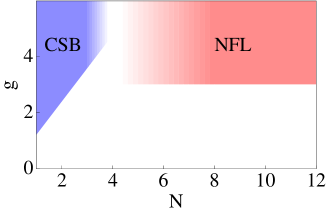
Figure 11: Phase diagram of the QED of 3D Dirac semimetals showing an approximate map of the phases corresponding to chiral symmetry breaking (CSB) and non-Fermi liquid behavior (NFL), obtained from the values of the respective critical couplings in the ladder approach and the large-$N$ approximation.

It is interesting to compare at this point the phase diagram in Fig. 11 with that obtained with the resolution of the Schwinger-Dyson equations, which can be trusted for all values of $N$. We can see from the results of Ref. qed that such a numerical approach sets indeed the interplay between the phases with chiral symmetry breaking and non-Fermi liquid behavior at $N=4$. For $N>4$, we observe that the critical line for that latter phase is not straight, although it approaches a constant asymptotic limit at large $N$. The self-consistent resolution leads also to a critical line for chiral symmetry breaking in the regime $N\leq 4$ that has an approximate linear behavior as a function of $N$. It is worth to mention that the values of the critical couplings found in the numerical resolution of Ref. qed are at first sight much larger than their counterparts in the diagram of Fig. 11. We have to bear in mind, however, that the critical values in that paper were given for the bare couplings, in the theory with a finite high-energy cutoff, while critical points like (75) and (113) are referred in the present context to the renormalized couplings. Overall, we may conclude that there is good qualitative agreement between the location of the phases in the diagram of Fig. 11 and in the more complete map obtained from the resolution of the Schwinger-Dyson equations.

We end up remarking that our analysis can be applied to characterize not only the strong-coupling regime of the 3D Dirac semimetals, but also of the Weyl semimetals. In these materials, each Weyl point hosts a fermion with a definite chirality, which means that the electron system cannot undergo chiral symmetry breaking through condensation of some order parameter at zero momentumhut . This obstruction does not hold however for the strong-coupling phase that we have identified in terms of the suppression of fermion quasiparticles. It is clear that the large-$N$ approach of Sec. IV applies equally well for Weyl and Dirac fermions, so that Weyl semimetals are susceptible of developing the phase with non-Fermi liquid behavior that we have mapped at large $N$ in the diagram of Fig. 11. In this respect, there should be good prospects to observe such an unconventional behavior in present candidates for Weyl semimetals, like TaAs or the pyrochlore iridates, which have up to 12 pairs of Weyl pointstaas1 ; taas2 . These considerations show that the strong-coupling phases studied here are not beyond reach, and that they may be actually realized in 3D Dirac or Weyl semimetals with suitably small values of the Fermi velocity or with the large number of fermion flavors already exhibited by known materials.

6 Acknowledgments

We acknowledge the financial support from MICINN (Spain) through grant FIS2011-23713 and from MINECO (Spain) through grant FIS2014-57432-P.

References

- (1) K. S. Novoselov, A. K. Geim, S. V. Morozov, D. Jiang, Y. Zhang, S. V. Dubonos, I. V. Grigorieva, and A. A. Firsov, Science 306 (2004) 666.
- (2) Z. K. Liu, B. Zhou, Y. Zhang, Z. J. Wang, H. M. Weng, D. Prabhakaran, S.-K. Mo, Z. X. Shen, Z. Fang, X. Dai, Z. Hussain and Y. L. Chen, Science 343, 864 (2014).
- (3) M. Neupane, S. Xu, R. Sankar, N. Alidoust, G. Bian, C. Liu, I. Belopolski, T.-R. Chang, H.-T. Jeng, H. Lin, A. Bansil, F. Chou and M. Z. Hasan, Nature Commun. 5, 3786 (2014).
- (4) S. Borisenko, Q. Gibson, D. Evtushinsky, V. Zabolotnyy, B. Büchner and R. J. Cava, Phys. Rev. Lett. 113, 027603 (2014).
- (5) S.-M. Huang, S.-Y. Xu, I. Belopolski, C.-C. Lee, G. Chang, B. Wang, N. Alidoust, G. Bian, M. Neupane, C. Zhang, S. Jia, A. Bansil, H. Lin and M. Z. Hasan, Nature Commun. 6, 7373 (2015).
- (6) S.-Y. Xu, I. Belopolski, N. Alidoust, M. Neupane, C. Zhang, R. Sankar, S.-M. Huang, C.-C. Lee, G. Chang, B. Wang, G. Bian, H. Zheng, D. S. Sanchez, F. Chou, H. Lin, S. Jia and M. Z. Hasan, report arXiv:1502.03807 (to appear in Science).
- (7) M. I. Katsnelson, K. S. Novoselov and A. K. Geim, Nature Phys. 2 (2006) 620.
- (8) H. Suzuura and T. Ando, Phys. Rev. Lett. 89 (2002) 266603.
- (9) M. Z. Hasan and C. L. Kane, Rev. Mod. Phys. 82, 3045 (2010).
- (10) X.-L. Qi and S.-C. Zhang, Physics Today 63, 33 (2010).
- (11) V. M. Pereira, J. Nilsson and A. H. Castro Neto, Phys. Rev. Lett. 99 (2007) 166802.
- (12) M. M. Fogler, D. S. Novikov, and B. I. Shklovskii, Phys. Rev. B 76 (2007) 233402.
- (13) A. V. Shytov, M. I. Katsnelson, and L. S. Levitov, Phys. Rev. Lett. 99 (2007) 236801.
- (14) I. S. Terekhov, A. I. Milstein, V. N. Kotov, and O. P. Sushkov, Phys. Rev. Lett. 100 (2008) 076803.
- (15) J. González, F. Guinea and M. A. H. Vozmediano, Nucl. Phys. B 424 (1994) 595.
- (16) J. González, F. Guinea and M. A. H. Vozmediano, Phys. Rev. B 59 (1999) R2474.
- (17) D. C. Elias, R. V. Gorbachev, A. S. Mayorov, S. V. Morozov, A. A. Zhukov, P. Blake, L. A. Ponomarenko, I. V. Grigorieva, K. S. Novoselov, F. Guinea and A. K. Geim, Nature Phys. 7 (2011) 701.
- (18) J. González, JHEP 08, 27 (2012).
- (19) O. V. Gamayun, E. V. Gorbar and V. P. Gusynin, Phys. Rev. B 80 (2009) 165429.
- (20) T. Maskawa and H. Nakajima, Prog. Theor. Phys. 52, 1326 (1974).
- (21) P. I. Fomin and V. A. Miransky, Phys. Lett. 64B, 166 (1976).
- (22) R. Fukuda and T. Kugo, Nucl. Phys. B 117, 250 (1976).
- (23) V. A. Miransky, Nuovo Cimento 90A, 149 (1985); Sov. Phys. JETP 61, 905 (1985).
- (24) V. P. Gusynin, Mod. Phys. Lett. A 5, 133 (1990).
- (25) K.-I. Kondo and H. Nakatani, Nucl. Phys. B 351, 236 (1991).
- (26) D. Atkinson, H. J. De Groot and P. W. Johnson, Int. J. Mod. Phys. A 7, 7629 (1992).
- (27) K.-I. Kondo, H. Mino and H. Nakatani, Mod. Phys. Lett. A 7, 1509 (1992).
- (28) J. González, Phys. Rev. B 90, 121107(R) (2014).
- (29) P. Ramond, Field Theory: A Modern Primer, Benjamin/Cummings, Reading (1981).
- (30) This scaling of the Fermi velocity in 3D Dirac semimetals has been pointed out by P. Hosur, S. A. Parameswaran, and A. Vishwanath, Phys. Rev. Lett. 108, 046602 (2012), and also by B. Rosenstein and M. Lewkowicz, Phys. Rev. B 88, 045108 (2013).
- (31) D. J. Amit and V. Martín-Mayor, Field Theory, the Renormalization Group, and Critical Phenomena, World Scientific, Singapore (2005).
- (32) This phase has been also studied in 3D Dirac semimetals by A. Sekine and K. Nomura, Phys. Rev. B 90, 075137 (2014).
- (33) J. Sabio, F. Sols and F. Guinea, Phys. Rev. B 82, 121413(R) (2010).
- (34) J. González, report arXiv:1502.07640 (to appear in Phys. Rev. B).
- (35) E. M. Lifshitz and L. P. Pitaevskii, Relativistic Quantum Theory (Course of Theoretical Physics Volume 4, Part 2), Pergamon Press, Oxford (1974).
- (36) Signatures of the breakdown of the Fermi liquid picture in the 3D Dirac semimetals have been also found by J. Hofmann, E. Barnes and S. Das Sarma, Phys. Rev. B 92, 045104 (2015).
- (37) P.-A. Bares and X. G. Wen, Phys. Rev. B 48, 8636 (1993).
- (38) C. Nayak and F. Wilczek, Nucl. Phys. B 417, 359 (1994).
- (39) A. Houghton, H.-J. Kwon, J. B. Marston and R. Shankar, J. Phys.: Condens. Matter 6, 4909 (1994).
- (40) C. Castellani, S. Caprara, C. Di Castro and A. Maccarone, Nucl. Phys. B 594, 747 (2001).
- (41) One cannot discard however the possible development of a condensate with nonvanishing momentum, as analyzed by R.-X. Zhang, J. A. Hutasoit, Y. Sun, B. Yan, C. Xu, and C.-X. Liu, report arXiv:1503.00358.