Light Bridge in a Developing Active Region.
II. Numerical Simulation of Flux Emergence and Light Bridge Formation

Abstract

Light bridges, the bright structure dividing umbrae in sunspot regions, show various activity events. In Paper I, we reported on analysis of multi-wavelength observations of a light bridge in a developing active region (AR) and concluded that the activity events are caused by magnetic reconnection driven by magnetconvective evolution. The aim of this second paper is to investigate the detailed magnetic and velocity structures and the formation mechanism of light bridges. For this purpose, we analyze numerical simulation data from a radiative magnetohydrodynamics model of an emerging AR. We find that a weakly-magnetized plasma upflow in the near-surface layers of the convection zone is entrained between the emerging magnetic bundles that appear as pores at the solar surface. This convective upflow continuously transports horizontal fields to the surface layer and creates a light bridge structure. Due to the magnetic shear between the horizontal fields of the bridge and the vertical fields of the ambient pores, an elongated cusp-shaped current layer is formed above the bridge, which may be favorable for magnetic reconnection. The striking correspondence between the observational results of Paper I and the numerical results of this paper provides a consistent physical picture of light bridges. The dynamic activity phenomena occur as a natural result of the bridge formation and its convective nature, which has much in common with those of umbral dots and penumbral filaments.

1 Introduction

Light bridges are bright features in white light separating umbral regions in sunspots. It is known that the light bridges typically have a weaker magnetic field compared to the ambient umbrae (Beckers & Schröter, 1969; Lites et al., 1991; Rüedi et al., 1995). They are associated with various activity phenomena including Ca II H brightenings and ejections (Louis et al., 2008; Shimizu et al., 2009), H$\alpha$ surges (Roy, 1973; Asai et al., 2001), and brightenings in TRACE 1600 Å channel (Berger & Berdyugina, 2003). Such phenomena may be caused by the interaction between the light bridge magnetic field and the external field that has a canopy structure (Leka, 1997; Jurčák et al., 2006).

The aim of this series of papers (this paper along with Toriumi et al. (2015), hereafter Paper I) is to reveal the nature of the light bridges that appear not in the fragmentation process of decaying sunspots but in the assembling phase of developing active regions (ARs) and the resultant occurrence of the activity phenomena. We approach this problem with a comparative study of observations and magnetohydrodynamic (MHD) modeling. In Paper I, we analyzed NOAA AR 11974 utilizing various observational data and investigated the magnetic and velocity structure of the light bridge and its relation with the corresponding activity events. As a result, we found in the photosphere that the light bridge in this developing AR has relatively weaker, almost horizontal field, while the surrounding pores have stronger, almost vertical field. As the AR continued to grow, the pores approached each other and coalesced into a single sunspot. While it existed, the bridge showed a large-scale convective upflow composed of smaller-sized cells and horizontal divergent outflow of a time scale of 10 – 15 minutes. Above the light bridge, a chromospheric (or upper-photospheric) brightening was intermittently and repeatedly observed with a typical duration of 10 – 20 minutes. In addition, repeated brightenings in the chromosphere preceded dark surges. These observational results led us to propose that magnetic reconnection driven by the magnetoconvection produces the activity phenomena. More precisely, the convective upflow in the light bridge repeatedly transports the weak horizontal fields to the surface layer, which then reconnects with the strong vertical fields of the surrounding pores, leading to the repetitive occurrence of the brightening and the surge ejections.

However, the observational study in Paper I leaves some open questions. For example, the formation mechanism of the light bridge is unclear. Although Katsukawa et al. (2007a) found that the light bridges in decaying sunspots formed as a chain of umbral dots, the bridge formation in the assembling phase of the nascent sunspots warrants further investigation. Another question is the driver of the large-scale flow structure inside the light bridge. Our photospheric observation showed that the bridge has a broad upflow with a flanking downflow. However, the vertical structure of the large-scale convection and its transportation of the magnetic flux remained unclear. Also, the existence of small-scale convection cells and the structure of total electric current needed further analysis.

Such questions may be answered by analyzing three-dimensional (3D) MHD simulations. In the last decade, the progress of realistic modeling of the solar magnetism using radiative MHD codes opened a new door to much better understanding of various features in the Sun. Among others, the MURaM code (Vögler et al., 2005; Rempel et al., 2009b), which takes into account the radiative energy transfer and the realistic equation of state, has been used extensively to model a variety of magnetic structures that are coupled with thermal convection, such as sunspot umbrae and umbral dots (Schüssler & Vögler, 2006), sunspots and penumbrae (Rempel et al., 2009a, b), emerging flux regions (Cheung et al., 2007, 2008), and AR formations (Cheung et al., 2010; Rempel & Cheung, 2014).

In Paper II, we provide the analysis of the MURaM simulation of an AR-scale flux emergence conducted by Cheung et al. (2010). In this simulation, the model proto-spots are accompanied by transient light bridges. Although the formation and disappearance of the light bridge were reported in Cheung et al. (2010), they did not pursue a detailed investigation of the light bridge. We present here an analysis of magnetic and flow structures of the model light bridge in their simulations within the context of the observations described in Paper I. The rest of this paper proceeds as follows. In Section 2, we describe the numerical simulation that we use, while in Section 3, we show the analysis results. Then, in Section 4, we discuss the comparison with observational results and the generality of magnetoconvection in a strong background magnetic field. Finally, in Section 5, we conclude with a synthesis of lessons learned from the two papers.

2 Numerical Simulation

In this study, we used the numerical results of the radiative MHD simulation of a large-scale flux emergence from the convection zone by Cheung et al. (2010). The simulation was conducted using the MURaM code. In this experiment, we set a 3D Cartesian computational domain of $92.16\ {\rm Mm}\times 49.152\ {\rm Mm}\times 8.192\ {\rm Mm}$, which is spanned by $1920\times 1024\times 256$ grid cells. The grid spacings are 48 km for both horizontal directions and 32 km for vertical direction. The base of the photosphere, which is defined as the mean height where the Rosseland optical depth becomes unity ($\tau=1$), is at $7.52\ {\rm Mm}$ above the bottom of the domain.

The emergence of a twisted flux tube was mimicked by kinematically inserting a twisted flux tube with the shape of a half torus (Fan & Gibson, 2003; Hood et al., 2009) through the bottom boundary into radiatively driven near-surface convective flows. The total magnetic flux contained in the flux tube is $7.6\times 10^{21}\ {\rm Mx}$, while the field strength averaged over the torus cross-section is 9 kG. After the half torus is completely inserted into the convection zone (about 5.9 hours after the start of inserting the flux tube), the bottom boundary is such that the subsurface roots of the tube are anchored. Magnetic field at the top boundary (about 670 km above the base of the photosphere) is matched to a potential field, whereas the periodic boundaries are assumed for both horizontal directions.

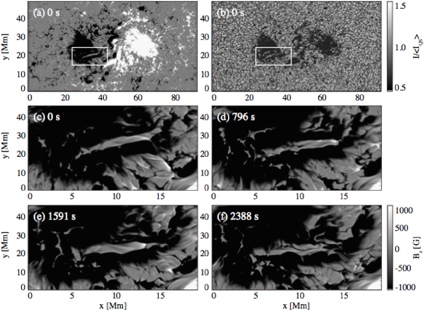
Figure 1: (a) Vertical magnetic field, $B_{z}$, at $t=0\ {\rm s}$ sampled at the base of the photosphere ($z=0\ {\rm Mm}$). (b) Continuum intensity map at the same time. (c–f) Sequential magnetogram showing the evolution of the light bridge structure. Field of view is indicated in panels (a) and (b) as a white box.

In this particular study, in order to obtain simulation outputs with a better temporal cadence, we restarted the calculation by using the original snapshot as the initial condition. The snapshot is taken at about 19 hours after the flux is inserted and we define this time as $t=0\ {\rm s}$. Figure 1(a) shows the surface vertical field of the entire computational domain (i.e., $\sim 92\ {\rm Mm}\times 49\ {\rm Mm}$) sampled at the constant height where $<\tau>=1$ at the time $t=0\ {\rm s}$. At this moment, the flux tube appears at the surface and creates a pair of strong flux concentrations, which are observed as pores (proto-spots) in the continuum intensity map (Figure 1(b)). Here, one may find that a partial light bridge structure is present in the negative polarity (see the white box in these figures). Figures 1(c) to (f) are the expanded view of this region, showing a temporal evolution of the light bridge for about 40 minutes. One can see that the light bridge has a much weaker field and is surrounded by the strong negative pores. Hereafter, we define 3D local coordinates $(x,y,z)$, where $z$ is anti-parallel with the gravitational acceleration and directed upward. The origin, $(x,y)=(0,0)$, is located at bottom left of the box in Figure 1(a), while $z=0$ is at the base of the photosphere (i.e., 7.52 Mm above the bottom boundary). We analyze the nature of this light bridge in detail in Section 3.

3 Results

3.1 Magnetic and Velocity Structures of the Light Bridge

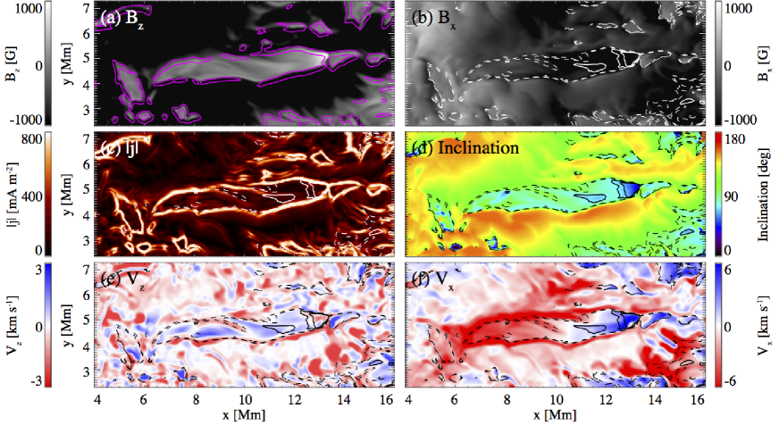
Figure 2: Maps for various physical parameters on the $z=0\ {\rm Mm}$ plane, measured at $t=1591\ {\rm s}$. (a) Vertical field $B_{z}$, (b) horizontal field $B_{x}$, (c) total electric current density $|\mbox{\boldmath$j$}|$, (d) inclination angle of the magnetic field with respect to the vertical direction, where $0^{\circ}$ is parallel to $\hat{\mbox{\boldmath$z$}}$, (e) vertical velocity $V_{z}$, where the positive value indicates upward, and (f) horizontal velocity $V_{x}$. In panel (a), purple contours show the current density of $|\mbox{\boldmath$j$}|=550\ {\rm mA\ m}^{-2}$. In the other panels, solid and dashed contours show $B_{z}=400\ {\rm G}$ and $200\ {\rm G}$ levels and $B_{z}=-200\ {\rm G}$ and $-400\ {\rm G}$ levels, respectively.

Figure 2 displays the maps for various physical quantities around the light bridge taken at the $z=0\ {\rm Mm}$ slice at the time $t=1591\ {\rm s}$. The light bridge has a weak vertical field $B_{z}$ (panel (a)) and field lines are much inclined to the negative $x$-direction (panels (b) and (d)). The surrounding pores have relatively stronger, more vertical fields ($B_{z}<-1000\ {\rm G}$: panels (a) and (d)). The bridge structure is clearly surrounded by a wall of the strong total electric current density (panels (a) and (c)),

$$|\mbox{\boldmath$j$}|=\left|\frac{1}{\mu_{0}}\nabla\times\mbox{\boldmath$B$}\right|,$$ (1)

where $\mu_{0}$ is the magnetic permeability. This is due to the magnetic shear between the inclined fields of the light bridge and the vertical fields of the ambient pores. From the electric current map, the size of the bridge is measured to be about $7.5\ {\rm Mm}\times 1.5\ {\rm Mm}$. In the vertical velocity map ($V_{z}$: panel (e)), within the light bridge, one may find a broad upflow region that is divided by narrower downflow lanes. That is, the light bridge contains several convection cells inside ($\sim 2\ {\rm Mm}\times 0.5\ {\rm Mm}$). At the edges of the bridge, narrow downflow lanes are also seen. The horizontal velocity $V_{x}$ distributions (panel (f)) show a divergent structure in the light bridge: $V_{x}$ is negative for $x\lesssim 10.5\ {\rm Mm}$ and is positive in the other side. However, at the light bridge boundary, $V_{x}$ shows a strong negative flow (up to $10\ {\rm km\ s}^{-1}$), even in the range of $x>10.5\ {\rm Mm}$.

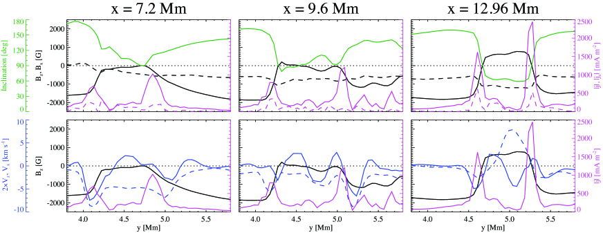
Figure 3: One-dimensional ($y$-)profiles across the light bridge on the $z=0\ {\rm Mm}$ surface, sampled at $x=7.2\ {\rm Mm}$, 9.6 Mm, and 12.96 Mm at $t=1591\ {\rm s}$. In upper panels, vertical field $B_{z}$ (black solid), horizontal field $B_{x}$ (black dashed), field inclination from the vertical (green), total electric current density $|\mbox{\boldmath$j$}|$ (purple solid), and vertical electric current density $|j_{z}|$ (purple dashed) are plotted. In lower panels, vertical velocity $V_{z}$ (blue solid) and horizontal velocity $V_{x}$ (blue dashed) are plotted along with vertical field $B_{z}$ (black) and total current $|\mbox{\boldmath$j$}|$ (purple). In all panels, horizontal dotted lines show the $B_{z}=B_{x}=V_{z}=V_{x}=0$ level.

Figure 3 shows 1D profiles of physical parameters sampled along the $y$-direction at three different $x$ positions ($x=7.2\ {\rm Mm}$, $9.6\ {\rm Mm}$, and $12.96\ {\rm Mm}$). It is remarkable at all three positions that the boundary of the bridge is clearly defined by the total current density $|\mbox{\boldmath$j$}|$, which is enhanced to $\gtrsim 500\ {\rm mA\ m}^{-2}$ because of the shear of magnetic fields inside and outside of the bridge. For comparison with the observations, we also plot the vertical component of the current $|j_{z}|$, which is derived only from the horizontal fields at a single layer,

$$|j_{z}|=\left|\frac{1}{\mu_{0}}\left(\frac{\partial B_{y}}{\partial x}-\frac{\partial B_{x}}{\partial y}\right)\right|.$$ (2)

Although $|j_{z}|$ is smaller than $|\mbox{\boldmath$j$}|$ by a factor of a few to 10, the peak positions of both quantities roughly overlap each other (see, in particular, the currents at $x=12.96\ {\rm Mm}$ in this figure). In observations, it is difficult to measure $|\mbox{\boldmath$j$}|$ since it requires the vertical variations of $B_{x}$ and $B_{y}$. However, the above result suggests that the vertical current $|j_{z}|$ serves as rather a reasonable indicator of the light bridge boundary. The value of the vertical current at the boundary is $|j_{z}|\gtrsim 100\ {\rm mA\ m}^{-2}$.

Note here that the vertical current $|j_{z}|$ in this plot is obtained from the horizontal derivatives of magnetic fields measured at a constant height in the simulation ($z=0\ {\rm Mm}$). In the actual observation (e.g., Paper I), however, the magnetic fields are measured at a constant-$\tau$ surface, whose geometrical height may fluctuate to some degree. We discuss this effect in Appendix A.

At the center of the light bridge at $x=9.6\ {\rm Mm}$, the vertical component of the magnetic field is very weak ($B_{z}\sim 0\ {\rm G}$) and the field is almost parallel to the solar surface ($B_{x}\sim-1000\ {\rm G}$; inclination $\sim 90^{\circ}$). The vertical velocity clearly shows two convective upflows ($V_{z}\sim 1.5\ {\rm km\ s}^{-1}$) that are separated by a downflow lane ($V_{z}\sim-2\ {\rm km\ s}^{-1}$). At this location, the horizontal flow is oriented to the negative $x$-direction ($V_{x}\sim-4\ {\rm km\ s}^{-1}$). At the edges of the bridge (around $y=4.2\ {\rm Mm}$ and $5.2\ {\rm Mm}$), both vertical and horizontal velocities are negatively enhanced ($V_{z}<-3\ {\rm km\ s}^{-1}$; $V_{x}<-8\ {\rm km\ s}^{-1}$) with total (absolute) velocity being up to $10\ {\rm km\ s}^{-1}$. The similar trend is seen in the leftmost end of the bridge at $x=7.2\ {\rm Mm}$. However, at this location, the vertical field falls below zero ($B_{z}\lesssim 0\ {\rm G}$) and thus the inclination becomes larger ($>90^{\circ}$). In contrast, at the rightmost end at $x=12.96\ {\rm Mm}$, the vertical field is intensified ($B_{z}>500\ {\rm G}$) and thus the inclination becomes smaller ($\sim 60^{\circ}$). The stronger magnetic shear around this site corresponds to the enhanced current density ($|\mbox{\boldmath$j$}|$ up to almost $2500\ {\rm mA\ m}^{-2}$). We can also find a stronger downflow ($V_{z}<-2\ {\rm km\ s}^{-1}$) with a positively enhanced horizontal velocity ($V_{x}\sim 8\ {\rm km\ s}^{-1}$). Outside of the bridge are the strong negative pores ($B_{z}\lesssim-1500\ {\rm G}$). The field is more vertical (inclination $>120^{\circ}$) and the vertical motion is suppressed ($V_{z}\sim 0\ {\rm km\ s}^{-1}$).

The cross-sectional (vertical) profiles of the light bridge at this time ($t=1591\ {\rm s}$) are shown in Figure 4. Here, we can see that the bridge takes root deeper in the convection zone (as dictated by the model bottom boundary). It has a large-scale upflow with a typical velocity of $V_{z}\sim 0.5\ {\rm km\ s}^{-1}$. Inside this upflow, the horizontal field $B_{x}$ is enhanced and the vertical field $B_{z}$ is reduced, resulting in a larger inclination angle ($\sim 90^{\circ}$). In this figure, surfaces of constant optical depth ($\tau$) are overplotted. It is clearly seen that the large-scale upflow lifts the iso-$\tau$ levels in the light bridge. Because of the radiative cooling, the rising material in the upflow region becomes denser and drains back to the convection zone at the edges of the bridge, forming a narrow downflow lane. This downflow is also seen at the center of the bridge, e.g., $(x,y,z)=(9.6\ {\rm Mm},4.7\ {\rm Mm},-0.1\ {\rm Mm})$, dividing the upflow region into two. This may account for the multi-cell structure observed in Figures 2 and 3. Moreover, the large-scale upflow turns into a divergent motion toward both $\pm x$-directions at the top $\sim 1.5\ {\rm Mm}$ layer in the convection zone. This outflow sweeps the magnetic flux in the $\pm x$-directions to the both ends of the light bridge, leading to the strong concentrations of the vertical flux at, e.g., around $x=13\ {\rm Mm}$. At this location, the $\tau=0.01$ layer is elevated to $z=500\ {\rm km}$.

In the $y$-$z$ slices of Figure 4, it is seen that the horizontal fields of the light bridge are surrounded by the strong downward fields of the ambient pores. Because of this magnetic shear, the electric current $|\mbox{\boldmath$j$}|$ forms a shell structure wrapping around the light bridge. The current layer clearly shows a cusp structure above the photosphere, which is created because the vertical fields of surrounding pores fan out over the light bridge (magnetic canopy: Leka, 1997; Jurčák et al., 2006). The $y$-$z$ current maps indicate that the enhancement of the current observed at the light bridge boundary in the photosphere of the actual Sun (e.g., Figure 3 of Paper I, ) is not due to the substantial change of the iso-$\tau$ levels around the bridge boundary. In other words, the observed strong current is not an observational artifact (see also Appendix A). In this figure (Figure 4), it is also interesting that the current layer overlaps with the fast uni-directional horizontal flow with $V_{x}=-5\ {\rm km\ s}^{-1}$ to $-10\ {\rm km\ s}^{-1}$, which is seen all along the light bridge boundary, even at the rightmost end ($x=12.96\ {\rm Mm}$).

From the above results, the magnetic and velocity structures of the present light bridge can be summarized as the “weakly-magnetized” intrusion of the convective upflow rather than the “field-free” intrusion. Although relatively weak, the light bridge still has a horizontal field of $B_{x}\sim-1000\ {\rm G}$ at the $z=0\ {\rm Mm}$ plane, which is roughly the same height as the raised $\tau=1$ surface. Also, it is seen that the light bridge that appears above the photosphere is only a top part of the deeper-rooted convective upflow. The cusp structure that we observe in the actual Sun may be just the tip of the iceberg.

3.2 Field-line Structure

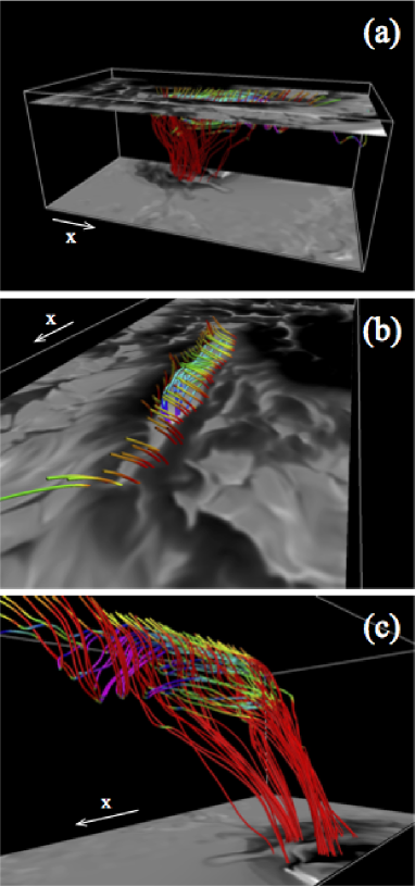
Figure 5: 3D visualization of magnetic field lines at the time $t=1591\ {\rm s}$. Seed points for the field lines are chosen in and around the light bridge structure observed at $z=0\ {\rm Mm}$. The color of the field lines represents the local vertical field strength $B_{z}$ ranging from $-1000\ {\rm G}$ (red) to $1000\ {\rm G}$ (purple). The upper horizontal plane is a magnetogram at the mean $\tau=1$ surface (i.e., $z=0\ {\rm Mm}$). The grayscale saturates at $-2000\ {\rm G}$ (black) and $2000\ {\rm G}$ (white). The lower plane is the same but near the bottom boundary ($z=-7.52\ {\rm Mm}$), saturating at $-20,000\ {\rm G}$ (black) and $20,000\ {\rm G}$ (white). In panel (c), the surface magnetogram is not shown.

Figure 5 shows the magnetic field-line connectivity in and around the light bridge structure. Here we use the VAPOR software package developed at NCAR (Clyne & Rast, 2005; Clyne et al., 2007) for plotting the data. The seed points for tracing the field lines are selected from the surface magnetogram, while the color indicates the local vertical field strength $B_{z}$. Panel (a) shows that all the field lines around the light bridge are connected to the flux concentration at the bottom boundary of the domain, which is one of the two footpoints of the twisted emerging flux tube inserted from the bottom boundary. In panel (b), we can see that the field lines in the light bridge (skyblue- and blue-colored fields) are highly inclined and are arching over or undulating around the surface. These structures are created by the local convective motions. It is remarkable that the field lines of the surrounding pores (red- and yellow-colored fields) fan out over the horizontal fields of the light bridge and form a canopy structure. The cusp-shaped current sheets between the bridge and the pores found in Figures 2, 3, and 4 are created by this magnetic shear.

In Figure 5(c), it is seen around the photosphere (upper part) that the horizontal field lines of the light bridge (skyblue to blue) are wrapped in the vertical fields of the pores (yellow to red). Interestingly, some of these vertical (pore) fields are connected to the horizontal (light bridge) fields with downward concave parts. This dip may be caused by the strong downflow at the light bridge boundary (see $y$–$z$ maps for $V_{z}$ in Figure 4). Also, this transition of the magnetic field from a vertical field with negative $B_{z}$ to a horizontal field with negative $B_{x}$, which exerts the Lorentz force (magnetic tension) partially in the negative $x$-direction, may be the driver of the fast horizontal flow in the negative $x$-direction at the light bridge boundary (see, e.g., Figure 2(f)). Similar concave magnetic fields are found in observations. Lagg et al. (2014) reported hints of magnetic field reversals at a bridge boundary, interpreting that the field lines are dragged down by fast downflows (see also Scharmer et al., 2013).

In the deeper interior, the field lines from the surface magnetic structures converge into two magnetic bundles, between which a weakly-magnetized region is trapped. This weakly-magnetized region has a weak upflow ($V_{z}<0.5\ {\rm km\ s}^{-1}$) and is connected to the light bridge in the upper layer. This structure indicates the close relationship among the flux emergence, the light bridge formation, and the eventual sunspot formation. Driven by the large-scale flux emergence, the two magnetic bundles approach each other in the convection zone, which is observed as the horizontal convergence of two pores at the solar surface (Zwaan, 1985; Strous & Zwaan, 1999). During this process, in the interior, the approaching magnetic bundles entrain the local upflow with weakly-magnetized plasma. As the upflow appears at the surface, the light bridge structure is created between the two ambient pores, which eventually form a single sunspot.

3.3 Flux Transportation in the Light Bridge

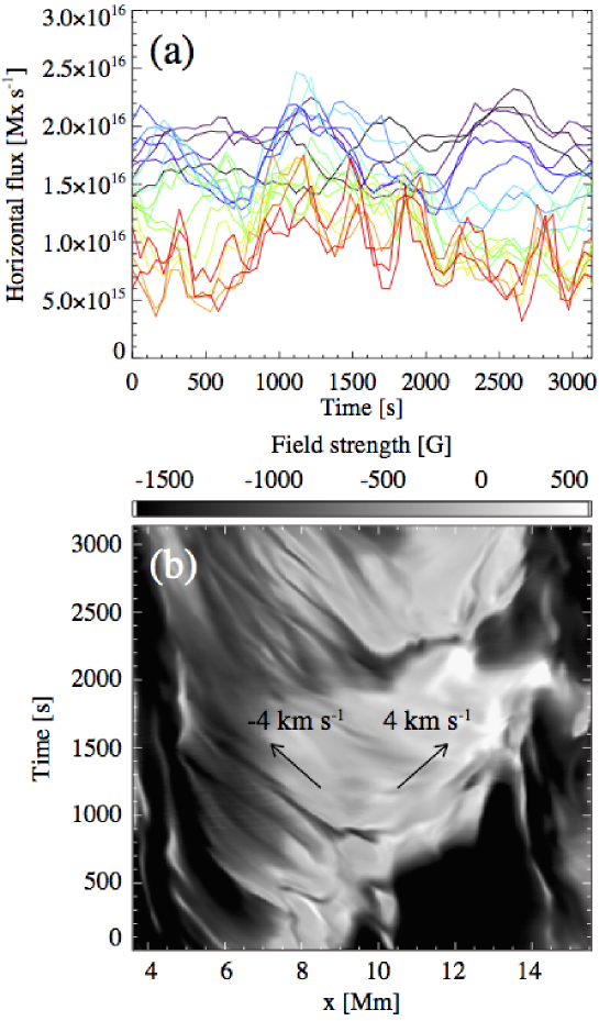
Figure 6: (a) Temporal evolution of the upwardly-transported unsigned horizontal flux (per unit time) $\Phi_{x}(z,t)$ (see text for details). Colors indicate the depths at which the flux is measured, ranging from $z=-3\ {\rm Mm}$ (black) to $z=0\ {\rm Mm}$ (red). (b) Temporal evolution of the vertical magnetic field $B_{z}$ at $z=0\ {\rm Mm}$ along the slit. The slit is placed at $y=4.8\ {\rm Mm}$, while arrows indicate the two different velocities.

In Section 3.1, we found that the large-scale convection pattern of the light bridge is a broad upflow accompanied by horizontal diverging flow (see Figures 2(e) and (f)). In order to examine whether this upflow transports the magnetic flux to the surface layer, we plot in Figure 6(a) emergence rate of horizontal flux that passes each depth level (per unit time) in the light bridge structure,

$$\Phi_{x}(z,t)=\int_{y_{1}}^{y_{2}}\left|B_{x}(z,t)\right|\,V_{z}(z,t)\,dy,$$ (3)

where $y_{1}=3.36\ {\rm Mm}$ and $y_{2}=6.24\ {\rm Mm}$. Note that the emergence rate is measured only within the upflow region ($V_{z}>0\ {\rm km\ s}^{-1}$), i.e., the measured value indicates the upwardly-transported horizontal flux. The solid lines in Figure 6(a) show temporal profiles of the flux transport at different depths, ranging from $z=-3\ {\rm Mm}$ (black) to $0\ {\rm Mm}$ (red). We can see from this figure that the flux is actually transported from the deeper layer to the surface, although only a fraction of the initial flux can reach the surface. For example, the measured flux at $z=0\ {\rm Mm}$ is about 50% of that at $z=-3\ {\rm Mm}$. The rest of the initial flux may return to the deeper layer in the downflow lane before reaching the photosphere. Also, a shorter-term fluctuation is noticeable in the profiles of the shallower layers, indicating that the time scale (and the size scale) of the convection becomes smaller with height. The typical period of this fluctuation is a few minutes.

As a result of the flux supply by the convective upflow, the flux continuously appears at the surface layer. Figure 6(b) illustrates the temporal evolution of the surface magnetic field $B_{z}$ along the $x$-slit placed at the center of the light bridge ($y=4.8\ {\rm Mm}$). This figure clearly shows that the separation of positive and negative polarities repeatedly occurs within the light bridge. The apparent speed of this diverging pattern is typically $\pm 4\ {\rm km\ s}^{-1}$, while the time scale of this pattern (the temporal gap between two consecutive trails) is a few to 10 minutes.

The V-shaped patterns in this slit-time diagram is due to the convective overturning (see, e.g., Figure 2(f)), which continuously advects the magnetic flux to both ends of the light bridge. In Figure 6(b), the positive (negative) polarities are seen to drift in the positive (negative) $x$-direction, which reflects the fact that the horizontal flux in the upflow region is oriented mostly to the negative $x$-direction (i.e., $B_{x}<0\ {\rm G}$). The apparent speed of $4\ {\rm km\ s}^{-1}$ is in good agreement with the actual horizontal velocity of about $4\ {\rm km\ s}^{-1}$ measured in Figure 3. Also, the time scale of a few to 10 minutes may reflect the shorter-term convection near the surface layer, which was found in Figure 6(a).

3.4 Response of the Atmosphere

It is known that the light bridges produce activity phenomena such as brightenings and surge ejections observed in chromospheric lines (see Section 1). The possible mechanism causing such phenomena is magnetic reconnection between the horizontal light bridge fields of the vertical umbral fields. Although we cannot reproduce the brightenings and ejections in the present simulation, which only captures the photosphere and near-surface convection zone, we can at least observe the response of upper layers of the photosphere.

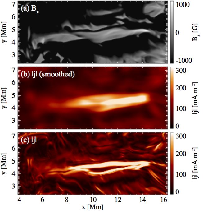
Figure 7: (a) Vertical field strength $B_{z}$ at $z=0\ {\rm km}$ at $t=1964\ {\rm s}$. (b) Total electric current density $|\mbox{\boldmath$j$}|$ averaged over $160\ {\rm km}\leq z\leq 480\ {\rm km}$ and smoothed for horizontal directions. (c) Same as (b) but without smoothing.

Figure 7 compares the photospheric context and the response in the atmosphere. Panel (a) shows the magnetogram $B_{z}$, while panels (b) and (c) are the total current density $|\mbox{\boldmath$j$}|$ averaged over the height range $160\ {\rm km}\leq z\leq 480\ {\rm km}$. Panel (b) shows the smoothed current and panel (c) is the original image. Here, the current in panel (b) exhibits a filamentary structure above the central line of the light bridge and is more enhanced in the right half ($x>10.5\ {\rm Mm}$) at this time. In the online movie, this filamentary structure evolves dynamically in association with the convective motion in the photosphere. The filamentary structure is seen simply because the two current layers around the light bridge are closer in the higher altitudes due to the cusp shape (panel (c), see also Figure 4). Since such a strong current is likely a place for heating, an elongated bright structure may be observed in upper atmosphere above the light bridge (say, in the chromosphere).

Magnetic reconnection, which may be observed as a sudden enhancement of the intensity, preferentially occurs at the places with a strong magnetic shear. In the present light bridge, the magnetic field is oriented mostly to the negative $x$-direction nd, thus, the right half of the bridge shows the positive polarities (Figure 6(b)). Therefore, the magnetic shear is stronger in the right half, which is reflected in the stronger currents in Figure 7(b). Cheung & Cameron (2012) found that the Hall effect in the weakly ionized photosphere is strongest at the cusp of the bridge, which may suggest that the cusp could be a preferred location for fast magnetic reconnection (Biskamp et al., 1995). In such a case, we conjecture that the intensity enhancement (heating of local plasma) and the surge ejection (cool plasma outflow launched from the reconnection site) are observed in the upper atmosphere. Since the horizontal field is supplied by the repetitive convection upflow as we saw in Section 3.3, the reconnection and the resultant intensity enhancement and surge ejection may occur repeatedly and intermittently in synchronization with the convection. In other words, the atmospheric activity is driven by the magnetoconvective dynamics in the solar interior.

3.5 Summary of the Numerical Results

In this section, we analyzed the numerical data of the convective flux emergence simulation focusing on the light bridge structure that appeared in one of the bipolar flux concentrations. The light bridge had a size of $\sim 7.5\ {\rm Mm}\times 1.5\ {\rm Mm}$ and was sandwiched between the strong pores of the negative polarity. The results obtained through a series of detailed analysis are summarized as follows:

• In the photosphere, the light bridge had a relatively weak field, which was highly inclined and almost horizontal to the solar surface. In the bridge center, the vertical component of the field strength was $B_{z}\sim 0\ {\rm G}$ with an inclination of $\sim 90^{\circ}$, oriented to the negative $x$-direction (i.e., $B_{x}<0\ {\rm G}$). In contrast, the surrounding pores had a strong negative polarity ($B_{z}\lesssim-1500\ {\rm G}$) and the field lines were more vertical. The magnetic shear between the horizontal fields of the light bridge and the vertical fields of the ambient pores formed a sharp current layer at the edges of the light bridge ($|\mbox{\boldmath$j$}|\gtrsim 500\ {\rm mA\ m}^{-2}$; $|j_{z}|\gtrsim 100\ {\rm mA\ m}^{-2}$). The bridge structure showed a broader upflow ($V_{z}\sim 2\ {\rm km\ s}^{-1}$) in its center, which was divided by downflow lanes into smaller convective cells ($\sim 2\ {\rm Mm}\times 0.5\ {\rm Mm}$). This broad upflow turned into the diverging, bi-directional motion of $V_{x}\sim\pm 4\ {\rm km\ s}^{-1}$. The light bridge also had a narrow downflow lane at its edge ($V_{z}<-3\ {\rm km\ s}^{-1}$). Along this edge, a rapid uni-directional flow of $V_{x}<-8\ {\rm km\ s}^{-1}$ was also observed.

• The light bridge took root deeper down in the convection zone and had a large-scale convective upflow ($V_{z}\sim 0.5\ {\rm km\ s}^{-1}$), which transports the weak horizontal fields to the solar surface (the “weakly-magnetized” intrusion). Surfaces of constant optical depth (iso-$\tau$ levels) were lifted by this upflow. The ascending plasma inside was radiatively cooled and became denser, turning back into the convection zone at the edges of the light bridge. The cross-sectional slices of the bridge showed a cusp structure, created due to the magnetic canopy of the surrounding pore fields.

• The magnetic field lines in the light bridge were highly inclined and had arched or serpentine structures, reflecting the local convection patterns. The horizontal fields were surrounded by the vertical fields of the neighboring pores. We found that some of the surrounding vertical fields were connected to the horizontal light bridge fields with a slight concave dip at the light bridge boundary. The dip may be created by the strong downflows at the boundary. Also, by exerting the magnetic tension force, this dip structure may drive the rapid uni-directional horizontal flow. With depth, the field lines in and around the light bridge converged into two flux bundles at the bottom boundary, between which a weakly-magnetized upflow was trapped. This means that, in the process of the merging of pores and the formation of a sunspot, the entrained upflow between the flux bundles (pores) appeared at the surface and formed the light bridge with supplying horizontal fields.

• We analyzed the transport of the horizontal fields by the light bridge upflow and found that only a fraction of the initial flux in the deeper layer reached the surface layer. The rest of the flux may return deeper down before reaching the surface. For the flux evolutions of the shallower layers, a short-term fluctuation was noticeable compared to those of the deeper layers. This is possibly due to the repeated appearance of shorter-lived, smaller-scale convection patterns near the surface. The upwardly transported horizontal fields were then guided by the lateral diverging flow. As a result of the flux advection, the vertical magnetic fields showed repeated separations of positive and negative polarities with an apparent speed of $V_{x}=\pm 4\ {\rm km\ s}^{-1}$ and a time scale of 10 minutes. The positive (negative) footpoints moved to the positive (negative) $x$-direction, which agreed with the fact that the horizontal fields were oriented to the negative $x$-direction.

• Magnetic reconnection between the transported horizontal fields in the light bridge and the pre-existing vertical fields of the umbral surroundings may be responsible for various dynamic phenomena observed in the light bridge. We found that the electric current of several 100 km above the light bridge is observed as a filamentary structure due to the cusp-shaped current sheet. The current was enhanced around the location where the magnetic shear is stronger. Such a place is preferable for the magnetic reconnection, which may be observed as a sudden intensity enhancement of the chromospheric lines. Since the magnetic flux is transported by the convective upflow in the light bridge, the brightening and the associated surge ejection may take place repeatedly and intermittently following the convective motion.

4 Discussion

4.1 Comparison with Observations

Figure 8 compares the light bridge observed in an actual AR in Paper I and that modeled in the present MHD simulation. The observation data were obtained by the spectropolarimeter of Hinode/SOT (Kosugi et al., 2007; Tsuneta et al., 2008; Lites et al., 2013; see Section 2.1 of Paper I for details). One may see that the structures of the bridges are remarkably consistent with each other: compare also Figures 3(g) and 4 of Paper I and Figures 3 and 6(b) of this paper. Table 1 summarizes various photospheric parameters. Except for the parameters representing the overall evolution (size and lifetime of the light bridge), the properties of the two cases agree well with each other. It should be noted here that the geometrical heights at which the photospheric parameters are measured are not necessarily the same. The parameters in the observation are measured using photospheric Fe I lines, which may geometrically fluctuate to some degree, while the parameters in the simulation are measured at a single horizontal plane at $z=0\ {\rm Mm}$. Also, in Table 1, the vertical velocity $V_{z}$ in the observation is actually a Doppler (line-of-sight) velocity. Nevertheless, the two cases show a striking correspondence, indicating that the numerical simulation captures some important physics of light bridges. The clear consistency of the physical quantities also indicates that we may be able to use the numerical results to estimate the physical states of the magnetic fields below and above the photosphere, which are difficult to directly observe.

Regarding the magnetic configuration above the photosphere, Leka (1997) and Jurčák et al. (2006) proposed a canopy structure above the light bridge. Our simulation results support their interpretation (Figures 4 and 5). Shimizu et al. (2009) reported strong electric current ($|j_{z}|>100\ {\rm mA\ m}^{-2}$) along a light bridge in the photosphere and long-lasting chromospheric jets intermittently and recurrently emanating from the bridge. They interpreted this enhanced current as a current-carrying, highly twisted flux tube that is trapped below a magnetic cusp, which reconnects with the surrounding vertical umbral field to trigger the chromospheric ejections (Nishizuka et al., 2012). Shimizu et al. (2009) observed another current enhancement, which they interpreted as a current sheet between the horizontal twisted flux tube and the vertical umbral field. In the present simulation, we also found two lanes of electric current of almost the same magnitude ($|j_{z}|\gtrsim 100\ {\rm mA\ m}^{-2}$). Contrary to the flux tube model by Shimizu et al. (2009), the present current layers are formed due simply to the magnetic shear between the vertical pore field and the horizontal bridge field, which is transported by a large-scale convective upflow. Chromospheric brightenings above the light bridge may be observed as a tube-like, filamentary structure as in Figure 7(b). However, we should take care that such a structure does not necessarily show the existence of the flux tube, as is indicated in Figure 7(c).

4.2 Magnetoconvection in a Strong Background Magnetic Field

From the observational and numerical results of this series of papers, we found that the light bridges have a convective upflow into a strong background magnetic field (“weakly-magnetized” intrusion). We suggested that the magnetic shear between the horizontal fields transported by this upflow and the vertical fields of ambient pores is essential for various activity events around the bridges. As was discussed earlier by Spruit & Scharmer (2006) and Rimmele (2008), similar magnetic and velocity structures are known to exist in the Sun, especially in sunspot regions.

One such example is umbral dots, the transient bright points in umbrae of sunspots. It is known that the umbral dots have upflows with weaker field (see Borrero & Ichimoto, 2011, and references therein). Parker (1979) and Choudhuri (1986) suggested that the umbral dots are the “field-free” intrusions of hot plasma into gappy umbral magnetic field. Schüssler & Vögler (2006) reported that, in their magnetoconvection simulation, bright, narrow upflow plumes (i.e. umbral dots) with adjacent downflows are produced in a strong vertical magnetic field. They found that the plumes have a cusp structure and are almost field-free.

Another example is penumbral filaments, the radially extended thin structures in sunspot penumbra. Observationally, the magnetic fields in the penumbra have two distinct inclinations interlaced with each other, which is referred to as “uncombed penumbra” (Solanki & Montavon, 1993) or “interlocking comb structure” (Thomas & Weiss, 1992). In the penumbra, radial outflow called Evershed flow is observed (Evershed, 1909). Moreover, Katsukawa et al. (2007b) found small-scale jetlike features (penumbral microjets), which are possibly caused by magnetic reconnection between the interlocking fields. In fact, the magnetoconvective pattern of the simulated penumbra is to a large extent similar to that of the light bridges in our present study (Rempel et al., 2009a, b; Rempel, 2011, 2012). Also, convective overturning motions similar to our cases have been found in the observations (see, e.g., Zakharov et al., 2008).

The similarities and consistencies among the umbral dots, light bridges, and penumbral filaments, which are summarized in Table 2, point to the generality of the magnetoconvection in a strong background field. Moreover, such a convection may produce variety of activity events through magnetic reconnection. Therefore, we can conclude that the magnetoconvection is not only a common physical phenomenon associated with the aforementioned features, but is also the essential driver of dynamic activity in sunspot regions.

5 Concluding Remarks

In this series of papers, we studied the nature of light bridges in newly developing ARs. From these studies, we present a consistent physical picture of light bridges based on both observations and numerical simulations.

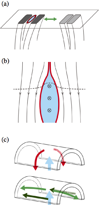
Figure 9: (a) Light bridge formation in an emerging flux region. Darker and lighter rounded rectangles are the pores, from which the magnetic fields are extended downward into the convection zone. On the left side, a light bridge structure is sandwiched between the pores. The brigade has a broad upflow region (blue) with a narrow downflow lane (red). Flux emergence shows a diverging motion (green arrow), which results in the coalescence of pores of the same polarities. (b) Cross-sectional view of the light bridge and the surrounding pores. The light bridge has an upflow (blue), which transports a horizontal magnetic flux to the surface layers. The iso-$\tau$ levels are elevated by this upflow: dashed line indicates the $\tau=1$ level. Narrow downflow lanes (red) are formed at the bridge boundary. Outside of the bridge are the vertical magnetic fields of the surrounding pores. (c) Illustration showing the convection patterns within the cusp structure. In the light bridge, the plasma shows an upflow (blue), which diverges and turns into downflows (red) at the bridge boundary. The upflow also diverges to the direction of the light bridge, showing a bi-directional flow (light green). At the bridge boundary, a fast uni-directional flow (dark green) is also formed.

The formation of a light bridge in an emerging flux region is shown in Figure 9(a). The magnetic fields emerge through the convection zone in the form of split multiple flux bundles, which are observed as fragment polarities (pores) in the photosphere (Zwaan, 1985). As the flux bundles emerge, weakly-magnetized local plasma with upflow is entrained between the bundles and appears as a light bridge at the visible surface. The pores of the same polarities merge together and, eventually, sunspots are formed.

As shown in Figure 9(b), the bridge has a deep convective upflow in its center, which carries horizontal magnetic fields to the surface layer. Due to the radiative cooling, the ascending plasma loses buoyancy and sinks down at the narrow downflow lanes. At the bridge boundaries, the magnetic shear between the horizontal fields of the bridge and the vertical fields of the ambient pores forms a strong electric current layer. Some external vertical fields are connected to the internal horizontal field at the bridge boundary with concave dips, which are caused by strong downflows. In the upper atmosphere above the light bridge, the external vertical fields fan out and form canopy structures.

Various activity phenomena come about as a natural result of the bridge formation. In the cusp-shaped current layer formed above the light bridge, magnetic reconnection takes place. The heating of local plasma is observed as intensity enhancements of chromospheric (or upper-photospheric) lines, while the reconnection outflow of cool, dense plasma is observed as dark surges ejected into the coronal heights. Since the horizontal flux is continuously provided by convection, the activity phenomena last longer with a periodic and intermittent nature.

The large-scale velocity structure is depicted in Figure 9(c). Along with the convection within the cross-section, the upflow turns also in the direction along the length of the bridge. The diverging (bi-directional) outflow transports the magnetic flux to both ends of the bridge. Interestingly, rapid uni-directional horizontal flows are observed, which may be driven by the bent field lines connecting external vertical fields and internal horizontal fields. In the shallower layers, smaller-scale, shorter-lived convection cells are superposed. As Cheung & Cameron (2012) pointed out, the Hall effect may generate the velocity and (as a result of advection) the magnetic field in the direction of bridge axis.

The above magnetoconvection scenario provides a unified perspective to wider variety of features in sunspot regions including umbral dots and penumbral filaments. All these features show a magnetoconvection in a strong background field. In fact, the magnetic and velocity structures of the light bridges, as well as the resultant activity events in the upper atmosphere, are remarkably similar to those of penumbral filaments (Rempel, 2012; Katsukawa et al., 2007b).

Although we have conducted a thorough investigation, we still have some remaining problems due to the limitations of the current analysis. Observationally, the magnetic structure at and around the magnetic reconnection that produces the activity phenomena is not determined. So far, Hinode data used in Paper I provides only a vector magnetogram at a single photospheric plane, which is lower than the expected reconnection site in the chromosphere or in the upper photosphere. Future missions may provide the detailed field information not only in the photosphere but also in the upper atmosphere. Another issue may be the dynamics of the weakly ionized plasma. In such altitudes, partial ionization effects such as the Hall effect and the ambipolar diffusion, which are not taken into account in the present simulation, may play important roles in the light bridge formation and the resultant reconnection (Leake et al., 2014; Martinez-Sykora et al., 2015). Future investigations with highly resolved simulations including these effects will further reveal the nature of the light bridge.

Appendix A Effect of Optical Depths

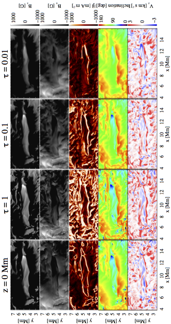
Figure 10: Physical parameters measured at a constant geometrical height ($z=0\ {\rm Mm}$) and three different iso-$\tau$ levels ($\tau=1$, $0.1$, and $0.01$).

Figure 10 shows various physical parameters measured at a constant geometrical height ($z=0\ {\rm Mm}$) and three different optical depths ($\tau=1$, $0.1$, and $0.01$). The general structure looks consistent with each other. According to Borrero et al. (2014), in deriving magnetic and velocity parameters, Milne-Eddington inversion codes generally sample shallower atmospheric layers (e.g., $\log{\tau}\sim-1.4$ for field strength, $\log{\tau}\sim-1.7$ for inclination, and $\log{\tau}\sim-1.0$ for line-of-sight velocity). Therefore, the Hinode observations in Figure 8 may be comparable to values at $\tau=0.1$ or $0.01$ in Figure 10.

In Section 3.1, we calculated the vertical current $|j_{z}|$ using horizontal derivatives of magnetic fields measured at a constant geometrical height ($z=0\ {\rm Mm}$). However, in the actual observations, magnetic fields are measured at constant-$\tau$ layers, which may fluctuate vertically. Therefore, the observational $|j_{z}|$ may be affected by such vertical fluctuations. In fact, as we saw in Figure 4, the iso-$\tau$ levels are lifted up substantially inside the light bridge because of the dense convective upflow.

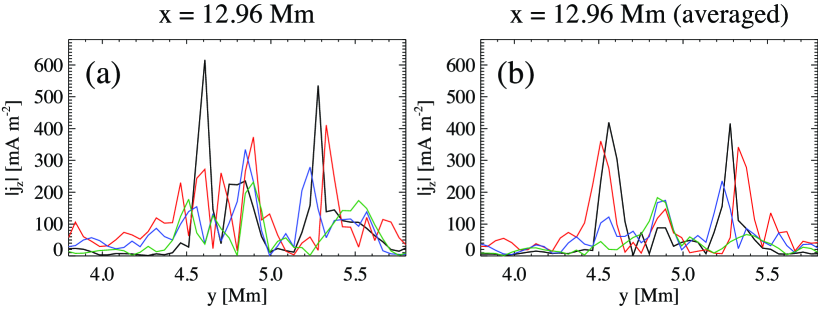
Figure 11: (a) Vertical current $|j_{z}|$ along $y$-axis (at $x=12.96\ {\rm Mm}$) derived from the horizontal magnetic fields measured at $z=0\ {\rm Mm}$ (black: corresponding to purple dashed line in Figure 3), $\tau=1$ (red), $\tau=0.1$ (blue), and $\tau=0.01$ (green). (b) Same as (a) but averaged from $x=12.72\ {\rm Mm}$ to $13.2\ {\rm Mm}$.

Figure 11(a) compares vertical currents computed from the horizontal fields measured at different layers. Although there are some fluctuations in the iso-$\tau$ currents, the peak locations and values roughly agree with the current measured at the $z=0\ {\rm Mm}$ level. Such agreements are clearer if we take averages over some range as in panel (b). Therefore, we can say that the observational $|j_{z}|$, which is derived from magnetic fields at a constant-$\tau$ layer, is still comparable to the actual $|j_{z}|$.

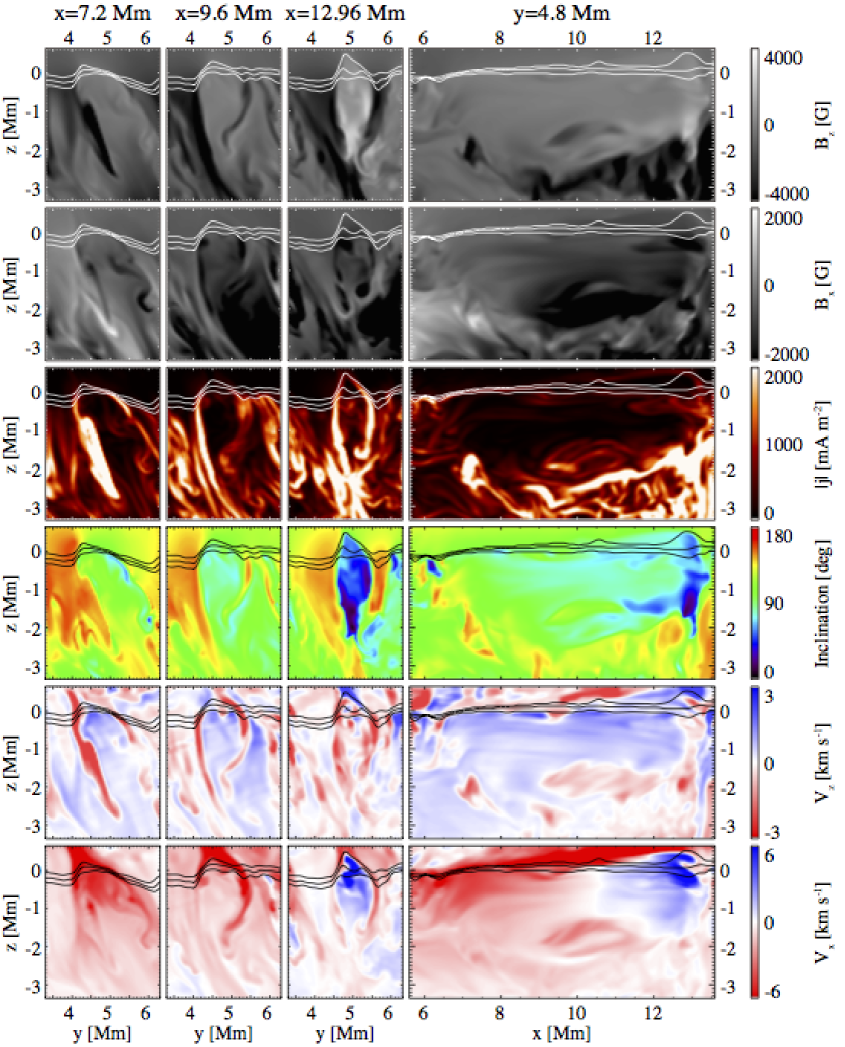
Figure 4: Cross-sectional vertical slices at $x=7.2\ {\rm Mm}$, $9.6\ {\rm Mm}$, $12.96\ {\rm Mm}$, and $y=4.8\ {\rm Mm}$ at the time $t=1591\ {\rm s}$. The panels show from top to bottom vertical field $B_{z}$, horizontal field $B_{x}$, total current density $|\mbox{\boldmath$j$}|$, inclination, vertical velocity $V_{z}$, and horizontal velocity $V_{x}$. The three solid lines in each panel indicate the $\tau=1$, $0.1$, and $0.01$ levels.

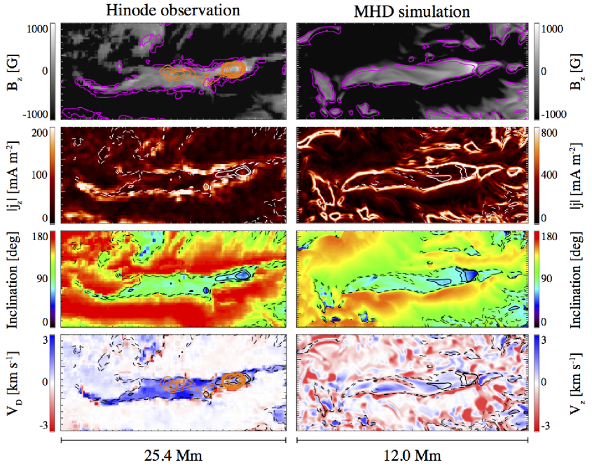
Figure 8: Comparison of the observed and simulated light bridges. (Left) Light bridge structure in NOAA AR 11974 observed by Hinode/SOT/SP. Figures are reproduced from Figure 3 of Paper I. From top to bottom, vertical field $B_{z}$, vertical current $|j_{z}|$, field inclination with respect to the local vertical, and Doppler velocity $V_{\rm D}$ are shown. Purple and orange contours indicate vertical currents and chromospheric intensity levels, respectively. Solid and dashed lines are $B_{z}=400\ {\rm G}$ and $200\ {\rm G}$ levels and $B_{z}=-200\ {\rm G}$ and $-400\ {\rm G}$ levels, respectively. See Paper I for details. (Right) Results of the MHD simulation carried out in this paper. Figures are reproduced from Figure 2. From top to bottom, vertical field $B_{z}$, total current $|\mbox{\boldmath$j$}|$, field inclination, and vertical velocity $V_{z}$ are shown. The physical values are sampled at $z=0\ {\rm Mm}$. Purple contours indicate the total current, while solid and dashed contours are the same as those in observation plots. See captions for Figure 2 for details.

Table 1: Comparison of Photospheric Parameters between the Observed and Modeled Light Bridges

Parameter	Hinode Observation	MHD simulation
Light bridge
Size	$\sim 22\ {\rm Mm}\times 3\ {\rm Mm}$	$\sim 7.5\ {\rm Mm}\times 1.5\ {\rm Mm}$
Lifetime	$\sim 2\ {\rm days}$	a few hours
$B_{z}$	$\sim 0\ {\rm G}$	$\sim 0\ {\rm G}$
$B_{x}$	$\sim-1000\ {\rm G}$	$\sim-1000\ {\rm G}$
Inclination	$\sim 90^{\circ}$	$\sim 90^{\circ}$
$V_{z}$	$\gtrsim 1\ {\rm km\ s}^{-1}$	$\sim 2\ {\rm km\ s}^{-1}$
$V_{x}$	a few km s-1	$\sim\pm 4\ {\rm km\ s}^{-1}$
Light bridge boundary
$V_{z}$	$\gtrsim-6\ {\rm km\ s}^{-1}$	$<-3\ {\rm km\ s}^{-1}$
$V_{x}$	$\cdots$	$<-8\ {\rm km\ s}^{-1}$
$|\mbox{\boldmath$j$}|$	$\cdots$	500 – $2500\ {\rm mA\ m}^{-2}$
$|j_{z}|$	$\gtrsim 100\ {\rm mA\ m}^{-2}$	$\gtrsim 100\ {\rm mA\ m}^{-2}$
Ambient pore
$B_{z}$	$\sim-2000\ {\rm G}$	$\lesssim-1500\ {\rm G}$
Inclination	$\sim 180^{\circ}$	$>120^{\circ}$
$V_{z}$	$\sim 0\ {\rm km\ s}^{-1}$	$\sim 0\ {\rm km\ s}^{-1}$

Note. — The heights at which the physical parameters are measured are not necessarily the same between the two cases. Vertical velocity $V_{z}$ in the observation is Doppler velocity.

Table 2: Characteristics and Activity Phenomena of Umbral Dots, Light Bridges, and Penumbral Filaments

	Umbral dots	Light bridges	Penumbral filaments
Circumstance	umbra	umbra/inter-pore	penumbra
Configuration	point-like	elongated	elongated
Flow structure	narrow upflow with	upflow, bi-directional outflow,	upflow, uni-directional outflow,
	adjacent downflows	and peripheral downflows	and peripheral downflows
Background field	vertical	vertical	inclined
Activity events	$\cdots$	brightenings/surges	microjets

References

- Asai et al. (2001) Asai, A., Shimojo, M., Isobe, H., et al. 2001, ApJ, 562, L103
- Beckers & Schröter (1969) Beckers, J. M. & Schröter, E. H. 1969, Sol. Phys., 10, 384
- Berger & Berdyugina (2003) Berger, T. E. & Berdyugina, S. V. 2003, ApJ, 589, L117
- Biskamp et al. (1995) Biskamp, D., Schwarz, E., & Drake, J. F. 1995, Physical Review Letters, 75, 3850
- Borrero & Ichimoto (2011) Borrero, J. M. & Ichimoto, K. 2011, Living Reviews in Solar Physics, 8, 4
- Borrero et al. (2014) Borrero, J. M., Lites, B. W., Lagg, A., Rezaei, R., & Rempel, M. 2014, A&A, 572, A54
- Cheung et al. (2007) Cheung, M. C. M., Schüssler, & M., Moreno-Insertis, F. 2007, A&A, 467, 703
- Cheung et al. (2008) Cheung, M. C. M., Schüssler, M., Tarbell, T. D., & Title, A. M. 2008, ApJ, 687, 1373
- Cheung et al. (2010) Cheung, M. C. M., Rempel, M., Title, A. M., & Schüssler, M. 2010, ApJ, 720, 233
- Cheung & Cameron (2012) Cheung, M. C. M. & Cameron, R. H. 2012, ApJ, 750, 6
- Choudhuri (1986) Choudhuri, A. R. 1986, ApJ, 302, 809
- Clyne et al. (2007) Clyne, J., Mininni, P., Norton, A., & Rast, M. 2007, New J. Phys., 9, 301
- Clyne & Rast (2005) Clyne, J., & Rast, M. 2005, Proc. SPIE, 5669, 284
- Evershed (1909) Evershed, J. 1909, MNRAS, 69, 454
- Fan & Gibson (2003) Fan, Y. & Gibson, S. E. 2003, ApJ, 589L, 105
- Hood et al. (2009) Hood, A. W., Archontis, V., Galsgaard, K., & Moreno-Insertis, F. 2009, A&A, 503, 999
- Jurčák et al. (2006) Jurčák, J., Martínez Pillet, V., & Sobotka, M. 2006, A&A, 453, 1079
- Katsukawa et al. (2007a) Katsukawa, Y., Yokoyama, T., Berger, T. E., et al. 2007, PASJ, 59S, 577
- Katsukawa et al. (2007b) Katsukawa, Y., Berger, T. E., Ichimoto, K., et al. 2007, Science, 318, 1594
- Kosugi et al. (2007) Kosugi, T., Matsuzaki, K., Sakao, T., et al. 2007, Sol. Phys., 243, 3
- Lagg et al. (2014) Lagg, A., Solanki, S. K., van Noort, M., & Danilovic, S. 2014, A&A, 568, A60
- Leake et al. (2014) Leake, J. E., DeVore, C. R., Thayer, J. P., et al. 2014, Space Sci. Rev., 184, 107
- Leka (1997) Leka, K. D. 1997, ApJ, 484, 900
- Lites et al. (2013) Lites, B. W., Akin, D. L., Card, G., et al. 2013, Sol. Phys., 283, 579
- Lites et al. (1991) Lites, B. W., Bida, T. A., Johannesson, A., & Scharmer, G. B. 1991, ApJ, 373, 683
- Louis et al. (2008) Louis, R. E., Bayanna, A. R., Mathew, S. K., & Venkatakrishnan, P. 2008, Sol. Phys., 252, 43
- Martinez-Sykora et al. (2015) Martinez-Sykora, J., De Pontieu, B., Hansteen, V. H., & Carlsson, M. 2015 (in prep)
- Nishizuka et al. (2012) Nishizuka, N., Hayashi, Y., Tanabe, H., et al. 2012, ApJ, 756, 152
- Parker (1979) Parker, E. N. 1979, ApJ, 234, 333
- Rempel & Cheung (2014) Rempel, M. & Cheung, M. C. M. 2014, ApJ, 785, 90
- Rempel et al. (2009a) Rempel, M., Schüssler, M., Cameron, R. H., & Knölker, M. 2009, Science, 325, 171
- Rempel et al. (2009b) Rempel, M., Schüssler, M., & Knölker, M. 2009, ApJ, 691, 640
- Rempel (2011) Rempel, M. 2011, ApJ, 729, 5
- Rempel (2012) Rempel, M. 2012, ApJ, 750, 62
- Rimmele (2008) Rimmele, T. 2008, ApJ, 672, 684
- Roy (1973) Roy, J. R. 1973 Sol. Phys., 28, 95
- Rüedi et al. (1995) Rüedi, I., Solanki, S. K., & Livingston, W. 1995, A&A, 302, 543
- Scharmer et al. (2013) Scharmer, G. B., de la Cruz Rodriguez, J., Sütterlin, P., & Henriques, V. M. J. 2013, A&A, 553, A63
- Schüssler & Vögler (2006) Schüssler, M. & Vögler, A. 2006, ApJ, 641, L73
- Shimizu et al. (2009) Shimizu, T., Katsukawa, Y., Kubo, M., et al. 2009, ApJ, 696, L66
- Shimizu (2011) Shimizu, T. 2011, ApJ, 738, 83
- Solanki & Montavon (1993) Solanki, S. K. & Montavon, C. A. P. 1993, A&A, 275, 283
- Spruit & Scharmer (2006) Spruit, H. C. & Scharmer, G. B. 2006, A&A, 447, 343
- Strous & Zwaan (1999) Strous, L. H. & Zwaan, C. 1999, ApJ, 527, 435
- Thomas & Weiss (1992) Thomas, J. H. & Weiss, N. O. 1992, in Sunspots: Theory and Observations, ed. J. H. Thomas & N. O. Weiss (NATO ASI, C 375; Dordrecht: Kluwer), 3
- Toriumi et al. (2015) Toriumi, S., Katsukawa, Y., & Cheung, M. C. M. 2015, ApJ, in prep
- Tsuneta et al. (2008) Tsuneta, S., Ichimoto, K., Katsukawa, Y., et al. 2008, Sol. Phys., 249, 167
- Vögler et al. (2005) Vögler, A., Shelyag, S., Schüssler, M., et al. 2005, A&A, 429, 335
- Zakharov et al. (2008) Zakharov, V., Hirzberger, J., Riethmüller, T. L. Solanki, S. K., Kobel, P. 2008, A&A, 488L, 17
- Zwaan (1985) Zwaan, C. 1985, Sol. Phys., 100, 397