Light Bridge in a Developing Active Region.
I. Observation of Light Bridge and its Dynamic Activity Phenomena

Abstract

Light bridges, the bright structures that divide the umbra of sunspots and pores into smaller pieces, are known to produce wide variety of activity events in solar active regions (ARs). It is also known that the light bridges appear in the assembling process of nascent sunspots. The ultimate goal of this series of papers is to reveal the nature of light bridges in developing ARs and the occurrence of activity events associated with the light bridge structures from both observational and numerical approaches. In this first paper, exploiting the observational data obtained by Hinode, IRIS, and Solar Dynamics Observatory (SDO), we investigate the detailed structure of the light bridge in NOAA AR 11974 and its dynamic activity phenomena. As a result, we find that the light bridge has a weak, horizontal magnetic field, which is transported from the interior by large-scale convective upflow and is surrounded by strong, vertical fields of adjacent pores. In the chromosphere above the bridge, a transient brightening occurs repeatedly and intermittently, followed by a recurrent dark surge ejection into higher altitudes. Our analysis indicates that the brightening is the plasma heating due to magnetic reconnection at lower altitudes, while the dark surge is the cool, dense plasma ejected from the reconnection region. From the observational results, we conclude that the dynamic activity observed in a light bridge structure such as chromospheric brightenings and dark surge ejections are driven by magnetoconvective evolution within the light bridge and its interaction with surrounding magnetic fields.

1 Introduction

Solar active regions (ARs) are known to produce a wide variety of dynamic phenomena from sub-arcsec events like Ellerman bombs (Ellerman, 1917) to catastrophic eruptions like solar flares and coronal mass ejections (Shibata & Magara, 2011). It is now widely accepted that such phenomena are the result of magnetic reconnection, the dynamic physical mechanism that changes magnetic topology and releases magnetic energy.

It is also known that light bridges, the bright structures dividing the dark umbrae of sunspots and pores into multiple smaller elements, produce many activity events in ARs. Light bridges typically have a weaker magnetic field compared to surrounding umbrae with field lines highly inclined and aligned along the long axis of the bridges (Beckers & Schröter, 1969; Lites et al., 1991; Rüedi et al., 1995; Leka, 1997). The magnetic fields around the light bridge have a canopy structure (Jurčák et al., 2006), which supports the theoretical model that the light bridges are the “field-free” intrusion of hot plasma into the umbral magnetic field (Parker, 1979; Choudhuri, 1986; Spruit & Scharmer, 2006) and recent numerical simulations of sunspots that apply radiative magneto-convection (Rempel et al., 2009; Cheung et al., 2010; Rempel, 2011). The canopy configuration may be responsible for dynamic phenomena observed in the higher atmosphere such as Ca II H brightenings and ejections (Louis et al., 2008; Shimizu et al., 2009; Louis et al., 2009), H$\alpha$ surges (Roy, 1973; Asai et al., 2001; Bharti et al., 2007), brightenings in the TRACE 1600 Å channel (Berger & Berdyugina, 2003), etc. Regarding the light bridge formation, Katsukawa et al. (2007) observed a mature sunspot with high spatial resolution and found that many umbral dots appear in the umbra of the spot. They rapidly intrude into the umbra and eventually form a light bridge that cuts across the umbra.

To a large extent, studies of light bridges focused on the fragmentation phase of decaying sunspots. However, it is known that light bridges appear also in the assembling process of nascent sunspots (Bray & Loughhead, 1964; Garcia de la Rosa, 1987). In this case, bridges are created between merging pores that eventually grow into a single spot. It is highly possible that the formation of such light bridges is closely connected to the large-scale flux emergence from the convection zone. From this point of view, the light bridge structure in a developing AR is not only a driver of various dynamic activity phenomena but also one of the most important keys to understand the flux emergence and the resultant spot formation.

The aim of this series of papers (this paper along with Toriumi et al. (2015), hereafter Paper II) is to reveal the nature of light bridges in newly emerging ARs and the occurrence of various activity events related to the light bridge structures from both observational and numerical perspectives. In the present paper, the first paper of the series, we analyze observations of NOAA AR 11974 to study the detailed structure of the light bridge that appeared during the course of spot formation and its relation with dynamic events that occurred in and around the light bridge. The organization of this paper is as follows. In Section 2, we describe the data that we used and give an overview of this AR. Then, in Sections 3 and 4, we show the analysis results of the light bridge and activity phenomena, respectively, which is followed by the summary of observational results in Section 5. We discuss the results in Section 6 and, finally, we conclude the paper in Section 7. Based on the observational results of the present work, in Paper II, we search for the formation process of a light bridge and the cause of activity events by analyzing numerical simulation data of AR formation (Cheung et al., 2010).

2 Observations

2.1 Observations and Data Reduction

For this analysis, we utilized observation data of the newly emerging NOAA AR 11974, which appeared on the southern hemisphere in February, 2014. In this subsection, we describe the observation data obtained by various instruments and their reduction processes.

The large-scale evolution in the photosphere is mainly covered by Helioseismic and Magnetic Imager (HMI; Scherrer et al. 2012; Schou et al. 2012) on board the Solar Dynamics Observatory (SDO; Pesnell et al. 2012). We used the tracked cutout data (line-of-sight (LOS) magnetogram, Dopplergram, and intensitygram) of AR 11974; the field-of-view (FOV) ranges $500\arcsec\times 250\arcsec$, which is enough for covering the entire AR. The duration is 3 hours from 22:00 UT, February 13. The pixel size and the time cadence are $0\farcs 50$ and 45 s, respectively. From the Dopplergram we subtracted the effect of the solar rotation, the orbital motion of the SDO satellite, and the east-west trend due to the spherical geometry of the Sun by applying the method introduced in Toriumi et al. (2014). We also used the SDO/Atmospheric Imaging Assembly (AIA; Lemen et al. 2012) data with the same FOV and duration as those of the HMI data to analyze the activity in the upper atmosphere. The data have a pixel size of $0\farcs 60$ for all bands and a cadence of 12 s for the extreme ultraviolet bands (EUV: 94 Å, 131 Å, 171 Å, 193 Å, 211 Å, 304 Å, and 335 Å), 24 s for the two ultraviolet bands (UV: 1600 Å and 1700 Å), and 3600 s for the continuum band (4500 Å). Both HMI and AIA data were exported from the Joint Science Operations Center (JSOC). They were mapped onto a common grid using the aia_prep routine in the SolarSoftWare package (Freeland & Handy, 1998).

During the period of the above-mentioned SDO data, the Solar Optical Telescope (SOT; Tsuneta et al. 2008) on board the Hinode satellite (Kosugi et al., 2007) tracked this AR and obtained Ca II H (3968.5 Å) broadband filtergram images with the FOV of $223\farcs 2\times 111\farcs 6$. The time cadence and the pixel size of this data are 1 minute and $0\farcs 218$, respectively. We calibrated the Ca data with the fg_prep procedure for dark-current subtraction and flat fielding. We also used the raster data of the spectropolarimeter (SP; Lites et al. 2013: two magnetically sensitive Fe I lines at 6301.5 Å and 6302.5 Å). In this time slot, there was one raster scan that starts at 00:00 UT and ends at 00:55 UT, February 14. The FOV is $255\farcs 8\times 122\farcs 9$ with the spatial sampling of $0\farcs 30$ and the step size of $0\farcs 32$. In this study we used the SOT/SP level 2 data, which are the outputs from the Milne–Eddington gRid Linear Inversion Network code (MERLIN; Lites et al. 2007). Note that the correction of orbital variation is done when the level 2 data are generated. The 180^∘ ambiguity in the azimuth angle of the magnetic field is resolved by using the AZAM utility (Lites et al., 1995).

Along with Hinode, the Interface Region Imaging Spectrograph (IRIS; De Pontieu et al. 2014) was also monitoring AR 11974 during this period. Here we used the IRIS data made from 22:14 UT, February 13, to 00:47 UT, February 14. This flarewatch program (OBS 3860259280) consists of repeated 8-step rasters with a step size of $2\farcs 0$. During the observation period there were 200 scans for the near-ultraviolet (NUV: 2790–2834 Å) and far-ultraviolet (FUV: 1333–1356 Å and 1399–1406 Å) wavelength bands and the first 122 scans were available. The pixel size is $0\farcs 167$ and the FOV for each scan is $14\farcs 1\times 119\farcs 4$. The step cadence and the raster cadence are 9.4 s and 75 s, respectively. At the same time, slit-jaw images (SJIs) in the filters of 1330 Å and 1400 Å were taken at a cadence of 19 s. The FOV is about $118\arcsec\times 118\arcsec$. We used the level 2 data, which take into account the dark-current subtraction, flat fielding, and geometrical correction.

The co-alignment among various observation data sets were achieved by using AIA images as a reference: For the HMI and SOT/SP data cross-correlations between the AIA 4500 Å image and the HMI intensitygram and SP Stokes-I image were used, while for the IRIS and SOT Ca data cross-correlations between the AIA 1600 Å images and the IRIS 1330 Å, 1400 Å, and Ca images were used.

2.2 Evolution of AR 11974 and Overview of Activity Phenomena

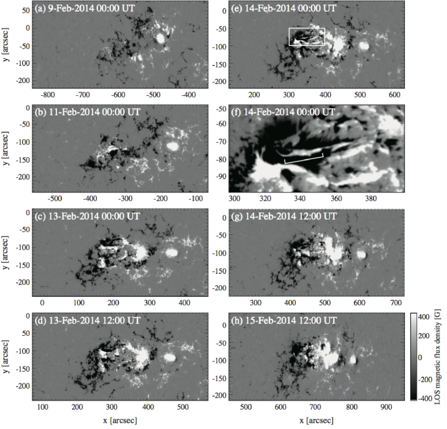
Figure 1: LOS magnetogram of NOAA AR 11974 obtained by SDO/HMI. White box in panel (e) indicates the FOV of panel (f). The light bridge structure sandwiched between two negative pores is shown in panel (f). In this figure, $(x,y)$ represent the heliocentric-Cartesian coordinates, where the origin $(0,0)$ is located at the disk center.

Figure 1 shows the long-term evolution of NOAA AR 11974. This AR appeared on the southeastern limb on 2014 February 5 and, since then, it showed significant flux emergence to the east of the pre-existing positive sunspot and formed a complex AR (panels (a) to (d)). From February 13, additional flux emerged within the AR, followed by the formation of a light bridge in the following polarity proto-spot (panel (e)). Panel (f) is the enlarged version of (e), which shows that an elongated structure (i.e. light bridge) has a weak positive LOS magnetic field and is sandwiched between two negative pores. The bridge has a length (extension along the long axis) of $\sim 30\arcsec\sim 22\ {\rm Mm}$ with a width (thickness across the bridge) of $\sim 4\arcsec\sim 3\ {\rm Mm}$. Throughout the evolution, emerged small-scale magnetic elements of the same polarity gradually coalesced into larger magnetic elements. In a similar manner, the two negative pores around the light bridge came closer to merge with each other and thus the bridge became squeezed out (panel (g)). On February 15, as shown in panel (h), the magnetic elements of this AR eventually built up two major sunspots of positive and negative polarities and, until this moment, the light bridge structure had completely disappeared. Thus, the lifetime of this light bridge is about 2 days.

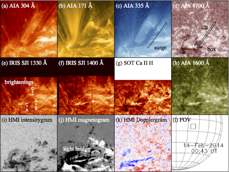
Figure 2: Composite of (a–d and h) AIA images, (e and f) IRIS SJIs, (g) SOT Ca image, and (i–k) HMI intensitygram, LOS magnetogram (saturating at $\pm 400\ {\rm G}$), and Dopplergram (saturating at $\pm 2\ {\rm km\ s}^{-1}$), all taken at around 00:43 UT, 2014 February 14. Panel (l) shows the location of the FOV (each panel has a $100\arcsec\times 100\arcsec$ FOV) and the time of the observation. Three continuous brightenings in the chromospheric images are marked as A, B, and C in panel (e), the dark surge is indicated in panel (c), and the light bridge is shown in panel (j). In panel (d), we show the locations of the slit and the box, which are used in the analysis in Section 4.2.

Together with flux emergence, the target AR 11974 showed a wide variety of dynamic phenomena. Figure 2 overviews the activity events in this AR. In panels (i) and (j), the light bridge structure is clearly seen between the negative polarity pores. This light bridge basically shows a blueshift indicating upward motion (panel (k)). In channels that image the photosphere and chromosphere (e.g., AIA 1600 Å and 1700 Å, IRIS 1330 Å and 1400 Å, and SOT Ca II H as in panels (d–h)), small-scale brightness enhancements are found to repeatedly occur in the middle of the FOV (see online movie). Here we mark three representative brightenings with A, B, and C. In addition, in the EUV images (panels (a–c)), a dark surge (jet) recurrently extends upward from the location of the light bridge, particularly from brightening A in the bridge (see movie). In the following sections, we describe these features in detail. The light bridge structure is analyzed in Section 3, while in Section 4 we investigate the brightenings and dark surges and reveal the correspondence with the bridge.

3 Magnetic and Velocity Structures of the Light Bridge

The recurrent brightening events (A) originate from positions coincident with the light bridge. Also, the dark surges recurrently stretch from the brightening events. This motivates us to investigate possible associations between the light bridge evolution and the brightening events. We first examine the detailed magnetic and velocity structures of the light bridge.

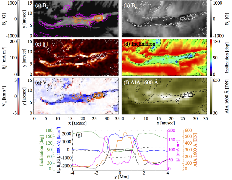
Figure 3: (a–e) SOT/SP data around the light bridge structure. This FOV is scanned westward from 00:16 to 00:23 UT, 2014 February 14. (a) Vertical magnetic field strength $B_{z}$. The vertical electric current density $|j_{z}|$ computed from $(B_{x},B_{y})$ is overlaid with purple contours. The contour levels are $|j_{z}|=100\ {\rm mA\ m}^{-2}$ and $200\ {\rm mA\ m}^{-2}$. In addition, AIA 1600 Å intensity at 00:20 UT is overlaid with orange contours. For the magnetic field, we use the local coordinates $(x,y,z)$, where $\hat{\mbox{\boldmath$z$}}$ is in the local radial direction. (b) Horizontal field strength $B_{x}$. Solid and dashed contours show $B_{z}=400\ {\rm G}$ and $200\ {\rm G}$ levels and $B_{z}=-200\ {\rm G}$ and $-400\ {\rm G}$ levels, respectively (same for panels (c–f)). (c) Vertical current density $|j_{z}|$. (d) Inclination angle of the magnetic fields with respect to the local vertical. (e) Doppler (LOS) velocity $V_{\rm D}$, where positive (blue) and negative (red) signs indicate the upward and downward velocity, respectively. Orange contours indicate the AIA 1600 Å intensity levels. (f) AIA 1600 Å intensity at 00:20 UT. (g) One-dimensional ($y$-)profiles across the light bridge averaged over $15\farcs 0\leq x\leq 22\farcs 5$. Black solid, black dashed, blue, green, and purple lines indicate vertical field strength $B_{z}$, horizontal field strength $B_{x}$, Doppler velocity $V_{\rm D}$, inclination angle of the magnetic field, and vertical electric current density $|j_{z}|$, all obtained from SOT/SP. Orange line indicates the AIA 1600 Å intensity at 00:20 UT, 2014 February 14. The origin of the $y$-axis is set at the middle between the two current ($|j_{z}|$) maxima, while the dotted line shows the $B_{z}=B_{x}=V_{\rm D}=0$ level.

Figures 3(a–e) show the SOT/SP data around the light bridge. Panel (a) is the vertical magnetic field strength $B_{z}$. For mapping the magnetic field, we use the local Cartesian reference frame $(x,y,z)$ with $\hat{\mbox{\boldmath$z$}}$ being the local radial direction. In Panel (a), the vertical field is overlaid by the absolute vertical electric current density contours $|j_{z}|$ (corresponding to panel (c)), where

$$|j_{z}|=\left|\frac{1}{\mu_{0}}\left(\frac{\partial B_{y}}{\partial x}-\frac{\partial B_{x}}{\partial y}\right)\right|$$ (1)

and $\mu_{0}$ is the magnetic permeability, and the AIA 1600 Å intensity contours (corresponding to panel (f)). Panels (b–d) are the maps for the horizontal field $B_{x}$, the vertical current $|j_{z}|$, the inclination angle with respect to the local vertical. Panel (e) shows the Doppler (i.e. LOS) velocity $V_{\rm D}$. In order to calibrate the absolute velocity, we subtracted the mean Doppler velocity calculated from the quiet Sun in the same SP data. Panel (f) shows the AIA 1600 Å intensity.

From Figures 3(a–d), we can see that the light bridge has an almost horizontal magnetic field with a lower strength ($B_{z}\sim 0\ {\rm G}$ and $B_{x}\sim-1000\ {\rm G}$) at the photosphere and is sandwiched between the strong, mostly vertical negative pores ($B_{z}\sim-2000\ {\rm G}$). We can also see that the enhancements of the vertical current ($|j_{z}|\gtrsim 100\ {\rm mA\ m}^{-2}$) are concentrated at the edges of the bridge. Photospheric magnetograms in a single layer do not allow us to compute horizontal components of the current to obtain the absolute current density $|\mbox{\boldmath$j$}|=|\nabla\times\mbox{\boldmath$B$}|/\mu_{0}$. Nevertheless, the observed distribution of $|j_{z}|$ suggests the presence of magnetic shear, which may be favorable for magnetic reconnection. It should be noted here that, since the magnetic fields are observed on the surface of a constant optical depth (iso-$\tau$ surface), $|j_{z}|$ may be affected by the vertical fluctuation of this surface. In Paper II, we analyze the simulation data and find that this effect is relatively small.

Figure 3(e) tells us that almost the entire light bridge shows upward motion ($V_{\rm D}\gtrsim 1\ {\rm km\ s}^{-1}$). In contrast, the edge of the bridge shows a downflow, which is much narrower and faster ($V_{\rm D}$ down to $-6\ {\rm km\ s}^{-1}$). Inside of the bridge, we can see localized patches of enhanced upflows ($V_{\rm D}>1.5\ {\rm km\ s}^{-1}$ with a size of $2\arcsec\times 1\arcsec$ to $3\arcsec\times 2\arcsec$). They seem to have a slightly elongated structure along the bridge. The brightenings in AIA 1600 Å (contours) are found in the middle of the bridge. Interestingly, the brightenings are located between the upflows of the convection cells: see, e.g., the brightening centered at $(x,y)=(17\arcsec,7\arcsec)$ and surrounding blue-shifted regions.

These observed properties are clearly seen in Figure 3(g), which shows the averaged profiles across the light bridge. Here, the vertical field $B_{z}$, Doppler velocity $V_{\rm D}$, field inclination from the vertical, vertical current density $|j_{z}|$, and the AIA 1600 Å intensity are plotted against the $y$-axis. The origin of the $y$-axis is set at the middle between the two maxima of the current $|j_{z}|$. In the light bridge ($|y|\lesssim 1\ {\rm Mm}$), the vertical field shows a plateau with relatively weaker, almost horizontal field ($B_{z}\sim 0\ {\rm G}$, $B_{x}\sim-1000\ {\rm G}$, inclination $\sim 90^{\circ}$). Therefore, the positive field seen in the light bridge structure in the HMI magnetogram (Figure 1(f) and Figure 2(j)) is mainly due to the projection effect caused because the bridge is located in the southwestern quadrant. The Doppler velocity shows an upflow ($V_{\rm D}\gtrsim 1.5\ {\rm km\ s}^{-1}$) in the bridge. At the same time, it also has two local humps around $y=\pm 0.8\ {\rm Mm}$, which clearly shows the existence of multiple convection cells in the bridge structure. The electric current is confined at the edges of the bridge ($|j_{z}|\gtrsim 100\ {\rm mA\ m}^{-2}$ at $y\sim\pm 1.3\ {\rm Mm}$), forming a clear boundary between the bridge and the surrounding pores. The downflows of the convection cells are concentrated just outside of the bridge boundary: see the slight dip in the Doppler velocity between $y=-1.2\ {\rm Mm}$ and $-1.8\ {\rm Mm}$ in this figure. In the pores ($|y|\gtrsim 1.5\ {\rm Mm}$), the magnetic field has a large negative value ($B_{z}\sim-2000\ {\rm G}$) and is more vertical, while the Doppler velocity is much weaker ($V_{\rm D}\sim 0\ {\rm km\ s}^{-1}$). The low-atmospheric brightening, AIA 1600 Å, peaks around $y=0.5\ {\rm Mm}$, i.e., middle of the light bridge. The peak of the brightening is spatially offset from the strong currents at the both edges and is located in between the two convective upflows, as is seen in Figures 3(a) and (e).

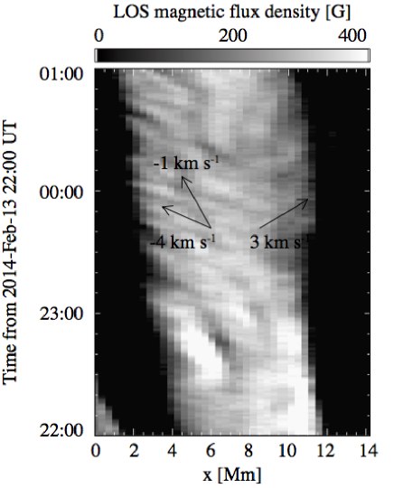
Figure 4: Slit-time diagram of the light bridge of HMI LOS magnetogram. The slit is set along the $x$-axis, which corresponds to $y=6\farcs 75$ over the range of $10\arcsec\leq x<30\arcsec$ in Figures 3(a–f). Arrows indicate three different velocities.

The temporal evolution of the light bridge is given in Figure 4, the time-sliced HMI magnetogram. The slit of this diagram is set along the $x$-axis, which is roughly parallel to the long axis of the bridge. In the eastern half of Figure 4 ($x\lesssim 8\ {\rm Mm}$), LOS magnetic fields show a coherent apparent motion to the east with a typical pattern velocity of $V_{x}=-1\ {\rm km\ s}^{-1}$ to $-4\ {\rm km\ s}^{-1}$. In contrast, the western half ($x\gtrsim 8\ {\rm Mm}$) shows a westward propagation with $V_{x}\sim 3\ {\rm km\ s}^{-1}$. In Figure 4, this divergent flow pattern continues at least for 2 hours and the typical time scale of the pattern is 10–15 minutes.

Combined with the Dopplergram of Figure 3(e), one can see that the large-scale, long-term velocity structure has an upflow in the light bridge, which turns into the divergent flow in the horizontal direction and finally sinks down at the narrow edge of the bridge. Superposed on this large-scale flow pattern are smaller-scale, shorter-lived convection cells with an elongated shape. The faint divergent magnetic pattern in Figure 4 suggests the continuous supply of weak magnetic flux from the solar interior, transported by the large-scale upflow of the light bridge.

4 Dynamic Activity Phenomena

4.1 Chromospheric Brightenings

In Figure 2, we found that a small-scale, intermittent brightening located at the western end of the light bridge (brightening A) repeatedly appear in the chromospheric images (AIA 1600 Å and 1700 Å, IRIS 1330 Å and 1400 Å, and SOT Ca II H). However, in this figure, similar brightenings can also be found outside of the bridge. In order to approach the cause of such brightening events in the chromosphere (or the upper photosphere), we then examine the spatial distribution and the spectral profiles of the brightenings.

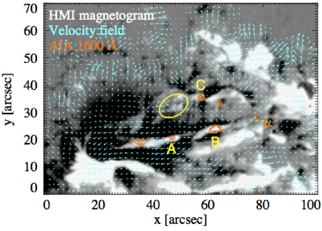
Figure 5: Horizontal velocity field (arrows) calculated from the sequential HMI magnetograms for 1 hour from 00:00 UT, 2014 February 14, plotted over the magnetogram at 00:43 UT (gray scale saturating at $\pm 400\ {\rm G}$). Orange contours indicate the $10\sigma$, $15\sigma$, and $20\sigma$ levels above the mean of AIA 1600 Å intensity at 00:43 UT. Three brightenings are denoted particularly by A, B, and C. Yellow ellipse shows one of the clear divergent regions, which indicates the flux emergence.

In Figure 5, we show the three intensity levels of AIA 1600 Å image ($10\sigma$, $15\sigma$, and $20\sigma$ above the mean calculated from the entire $500\arcsec\times 250\arcsec$ FOV, where $\sigma$ denotes the standard deviation) at 00:43 UT on 2014 February 14 (corresponding to Figure 2(h)) plotted on the HMI magnetogram taken at the same time (00:43 UT: corresponding to Figure 2(j)). One may see from Figure 5 that the brightening events are, in many cases, located at the mixed polarity regions, where the positive and negative polarities lie next to each other. For example, brightening A is located on the western end of the light bridge, where the weak positive LOS magnetic field is trapped between the neighboring negative polarities in the north and the south. Similarly, brightening B is also on the elongated positive (LOS) field, which is facing the negative fields at the northern and southern edges.

Apart from these two events (A and B), brightening C is located in between the positive and negative polarities. The arrows in Figure 5 show the averaged horizontal velocity field that is derived from the sequential HMI magnetograms between 00:00 UT and 01:00 UT, 2014 February 14, using the local correlation tracking (LCT) method (November & Simon, 1988). Here, the positive polarity at the location of brightening C is a new magnetic field sourced from a divergent region, i.e., an emerging flux region in the southeast (indicated by yellow ellipse). This newly emerging positive field collides into the pre-existing negative field and they cancel each other at this location. It should be noted here that this local flux emergence may also be responsible for the merging of negative pores surrounding the light bridge structure: this flux emergence produces the pore in the north of the light bridge and presses the pore against the bridge (see Figure 1 and Section 2.2).

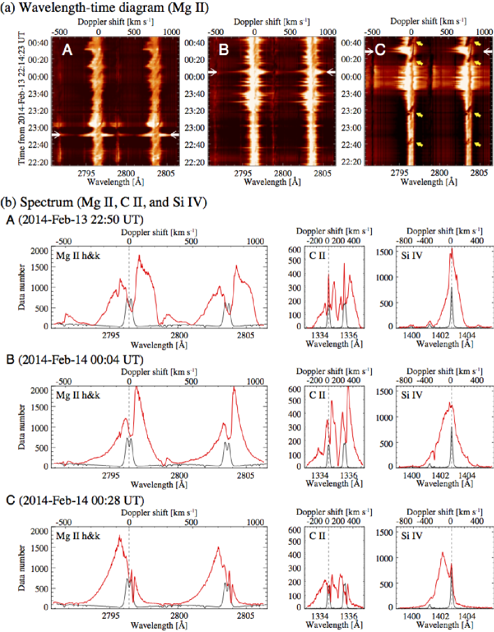
Figure 6: IRIS spectra for the three brightening events. (a) Wavelength-time plots of Mg II h & k for brightenings A, B, and C. Each diagram shows a temporal evolution in a single spatial pixel of the IRIS raster scan. The top axis shows the Doppler shift relative to the rest wavelength of Mg II k3. Yellow arrows indicate the dark transitions (see text for details). (b) Profiles of the three lines (Mg II, C II, and Si IV) for the three events. Black lines show the averaged quiet-Sun spectra, while red lines show the profiles at the selected times indicated by white arrows in (a). Here, the quiet-Sun profiles of C II and Si IV are multiplied by factors of 2 and 10, respectively.

Figure 6 shows the IRIS spectra for the three brightening events. In the wavelength-time plots (panel (a)), we can see that each intensity enhancement occurs repeatedly and frequently at the same location. The occurrence rate of the brightening is, for example in case B, once every few minutes. Panel (b) shows the spectra at the time of brightenings for three different lines (Mg II, C II, and Si IV) and the referential averaged quiet-Sun spectra, which are obtained from the less active area within the FOV of the same IRIS observation. The central reversal in the Mg II reference profiles is the self-absorption due to large opacity. Here, the spectra at A and B are intensified compared to the quiet-Sun profiles and are broadened toward both red and blue wings. These higher amplitude and broadened profiles are similar to the recent IRIS observation of brightening events at the flux cancellation sites in an emerging AR (Peter et al., 2014) and the Ellerman bombs (Vissers et al., 2015). Such spectral profiles are, in many cases, interpreted as the local heating of chromospheric plasma via magnetic reconnection and the bi-directional outflow from the reconnection region (e.g., Peter et al., 2014). Therefore, it is also possible that the enhanced and broadened profiles seen in Figure 6 represents the energy releasing by magnetic reconnection. This interpretation is further supported by the spatial distribution of the brightening events. In Figure 5, the brightenings were found to exist in the mixed polarity regions and some of them showed flux cancellation, which also indicates that the brightenings are caused by magnetic reconnection.

In contrast, IRIS spectral profiles of brightening C in Figure 6(b) look different from those of A and B. For instance, the Mg II profile of brightening C is seemingly single-peaked showing a strong upflow ($\sim-70\ {\rm km\ s}^{-1}$: blue-shifted) rather than the double-peaked profile of events A and B with clear central reversals. Upon closer inspection, however, one finds that the spectrum does have a central reversal with another dip on the red side of the reversal. Here, the Doppler shift of the dip from the rest wavelength of the line center is $+32.7\ {\rm km\ s}^{-1}$ (red-shifted), while the central reversal is located at $+5.5\ {\rm km\ s}^{-1}$ (red-shifted). A similar dip is also seen in the C II spectrum. This anomalous dip corresponds to the dark feature (intensity reduction) in the wavelength-time plot (marked by yellow arrows in panel (a)). This feature appears repeatedly with a lifetime of 10–20 minutes (four events: 22:39–22:47 UT and 23:13–23:25 UT on February 13 and 00:16–00:38 UT and from 00:35 UT on February 14), each time showing a sudden appearance of the blue shift and a smooth transition from the blue to the red side. We will discuss the cause of this anomalous intensity reduction in Section 4.2.

4.2 Ejection of Dark Surges

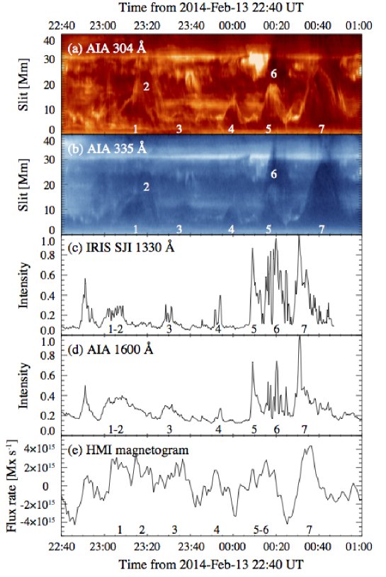
Figure 7: Slit-time evolution for (a) AIA 304 Å and (b) AIA 335 Å images, normalized lightcurves for (c) IRIS SJI 1330 Å and (d) AIA 1600 Å, and (e) the (smoothed) flux “decay” rate $-d\Phi/dt$ measured using HMI magnetogram (see text for details). The slit used in (a) and (b), which is shown by a rectangle in Figure 2(d), has a width of $2\farcs 5$ and the AIA intensities are averaged over the width. The lightcurves in (c) and (d) and the flux rate in (e) are measured within the box shown also in Figure 2(d). The size of the box is $3\arcsec\times 3\arcsec$. In each panel, we numbered 7 events to provide better correspondence.

In the EUV images of Figure 2, we found the recurrent ejection of a dark surge (jet) from the light bridge, especially from brightening A. In order to investigate the nature of the dark surges, along with its relationship with the chromospheric brightenings and the magnetic field of the light bridge, we examine the temporal evolutions of the surge, the brightening, and the surface magnetic field. In Figures 7 (a) and (b), we plot the time-slit diagrams for the two EUV images (AIA 304 Å and 335 Å), where the slit is set along the surges as indicated in Figure 2(d). One can see from Figures 7(a) and (b) that there is a recurrent extension of dark features (i.e., surges) with a typical lifetime of 10–20 minutes. The observed surges have a parabolic trajectory, which indicates that the ejected material is impulsively accelerated upward and decelerated by gravity. In all EUV channels, the surges are seen in absorption, implying that the material is cool and dense. However, in some channels such as AIA 304 Å in Figure 7(a), the front of each surge (the rim of the parabolic profile) appears in emission.

Table 1 summarizes the properties of the surges (lifetime, length, and acceleration). The length parameter in this table is defined as the maximum spatial extension of each surge along the slit in Figure 7(b), which is not necessary the same as the maximum height of the surge because of the projection effect and the inclination of the surge. Also, we calculated the acceleration of the surge from the length and lifetime as $a_{\rm DS}=8L_{\rm DS}/t_{\rm DS}^{2}$, where $a_{\rm DS}$, $L_{\rm DS}$, and $t_{\rm DS}$ are the acceleration, length, and lifetime of the dark surge, respectively, under the assumption that the launched plasma is decelerating at a constant rate. The obtained accelerations ($1.1\times 10^{4}\ {\rm cm\ s}^{-2}$ to $4.0\times 10^{4}\ {\rm cm\ s}^{-2}$) are of the same order of magnitude as the surface gravity ($2.7\times 10^{4}\ {\rm cm\ s}^{-2}$) indicating the gravitational deceleration.

In Figures 7(c) and (d), we plot the normalized lightcurves at the brightening A for the two UV images, IRIS 1330 Å SJI and AIA 1600 Å, respectively. The lightcurves are measured within the box of the size of $3\arcsec\times 3\arcsec$ indicated in Figure 2(d). Here, the brightening events have a duration of 10–20 minutes and, at the same time, the lightcurves show much more rapid fluctuations of a time scale over 3–5 minutes. Compared to the EUV images (Figures 7(a) and (b)), it is remarkable that each intensity enhancement in the lightcurves occurs just prior to the dark surge ejection (compare the numbered events in these panels of Figure 7). In each event, the lightcurve reaches its maximum about 5–15 minutes before the surge attains its maximum length. This temporal relationship suggests the causality between the chromospheric brightenings and the dark surges.

Table 1 lists the duration and the maximum normalized intensity of each brightening event measured from the AIA 1600 Å lightcurve (Figure 7(d)). For evaluating these values, we do not use IRIS SJI data (panel (c)) since SJI contains the slit and some contamination (see Figures 2(e) and (f)) and, in case of strong brightenings, some saturated pixels. These factors may be reflected in the IRIS SJI lightcurve.

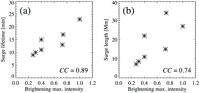
Figure 8: Correlations among brightening and surge parameters shown in Table 1. Correlation coefficient (linear Pearson correlation coefficient, $CC$) is indicated in the bottom right of each panel.

The relationship between the two dynamic phenomena in the light bridge, i.e., the brightenings and the surges, can be found in Figure 8. This figure shows the correlations among parameters in Table 1, the maximum normalized intensity of the brightenings and the lifetime and length of the surges. They show good correlations: the corresponding correlation coefficients (linear Pearson correlation coefficient, $CC$) for panels (a) and (b) are $CC=0.89$ and $0.74$, respectively. That is, the length and lifetime of the surges become larger with the brightening intensity. Although we have only a sample of 7 event pairs, these good correlations clearly point to the physical relationship between the brightenings and the dark surges.

In Section 4.1, based on the spatial distribution of the brightening events and their IRIS spectral profiles, we interpreted the cause of the brightenings as magnetic reconnection. Figure 7(e) may provide further support to this interpretation. This diagram shows the flux “decay” rate $-d\Phi/dt$, where $\Phi$ is the unsigned total magnetic flux,

$$\Phi=\int_{S}|B_{\rm LOS}|\,ds,$$ (2)

$B_{\rm LOS}$ is the LOS magnetic flux density in the HMI magnetogram, and $S\,(=3\arcsec\times 3\arcsec)$ is an area of the box in which the brightening lightcurves (i.e., Figures 7(c) and (d)) are measured. This decay rate is positive when the total magnetic flux decreases. In Figure 7(e), it is clearly seen that the flux rate becomes positive around the timing of brightening events. In contrast, when there is no prominent brightening, the decay rate remains negative. This trend indicates that the magnetic flux is continuously supplied to this region and is consumed during the brightenings, which we think is the magnetic reconnection (flux cancellation). As a result of the repeated reconnection, the plasma is ejected upward to create the recurrent dark surges.

The IRIS wavelength-time diagram of Mg II (Figure 6(a)) at location C shows smooth transitions of intensity reduction from blueshift to redshift relative to the rest wavelength of the line core (see Section 4.1). By comparing this figure with Figures 7(a) and (b), one may notice the temporal correspondence between the intensity reductions and the dark surges. For example, the three reductions starting at 23:13 UT on February 13 and 00:16 UT and 00:35 UT on February 14 occur almost at the same times as the surges numbered 2, 6, and 7. Also, both types of features (the intensity reduction and the dark surge) persist for 10–20 minutes. In addition to that, in the EUV time-slit diagrams of Figures 7(a) and (b), these three surges (2, 6, and 7) are the only events that go beyond the location of the brightening C, which is around 15–17 Mm on the slit but is not seen in the EUV channels. Therefore, from the temporal and spatial correspondence, we can expect that the repeated intensity reductions in the IRIS spectrum of brightening C to be caused by the recurrent dark surges that passed over and occulted the brightening along the IRIS LOS. The smooth transition from the blueshift to the redshift may indicate that the surge changes from the ascending to descending motion. We can furthermore see that the dark surges reach chromospheric temperatures, e.g., 10,000 K for Mg II (De Pontieu et al., 2014).

5 Summary of Observational Results

In the previous sections, we analyzed the light bridge structure in the developing AR 11974 and the activity phenomena around the bridge. The light bridge had a size of $\sim 22\ {\rm Mm}\times 3\ {\rm Mm}$ with a lifetime of $\sim 2$ days and was surrounded by merging negative polarity pores. Images in the AIA 1600 Å and 1700 Å, IRIS 1330 Å and 1400 Å SJI, SOT Ca II H channels showed small-scale intermittent brightenings, while the EUV data (AIA 304 Å, 171 Å, 335 Å, etc.) revealed the recurrent ejection of dark surges. By conducting the series of detailed analysis, we found the following:

• Photospheric magnetic field in the light bridge was relatively weaker ($\sim 1000\ {\rm G}$) and almost horizontal, while the surrounding pores showed strong ($\sim 2000\ {\rm G}$), almost vertical fields of the negative polarity. Because of the magnetic shear between the bridge and the pores, the boundary layer had a strong vertical current ($\gtrsim 100\ {\rm mA\ m}^{-2}$) in the photosphere, which is a favorable site for magnetic reconnection. The vertical motion in the light bridge was basically upward ($\gtrsim 1\ {\rm km\ s}^{-1}$), while the narrow edges showed strong downflows (down to $-6\ {\rm km\ s}^{-1}$). At the same time, the bridge showed the existence of multiple smaller-sized convection cells inside ($>1.5\ {\rm km\ s}^{-1}$; $\sim 2\arcsec\times 1\arcsec$ to $3\arcsec\times 2\arcsec$). It was found that the chromospheric (or upper-photospheric) brightenings were located in the middle of the bridge, i.e., deviated from the location of photospheric currents. Also, the brightenings were seen in between the small-scale upflows. These results show that the large-scale, long-term velocity structure of the light bridge is driven by an upflow, which then turns into the horizontal divergent motion ($V_{x}$ being $\pm$ a few km s^-1) and finally sinks down at the narrow edge of the bridge. The faint divergent pattern of magnetogram indicates the existence of continuous supply of magnetic flux by the large-scale upflow. The typical timescale of the propagation pattern was 10–15 minutes.

• The chromospheric brightenings occurred in the mixed polarity regions, some of which showed flux cancellation. For example, brightening A was on the western end of the light bridge of weak positive LOS fields, which was facing the surrounding negative pores. Brightening B had a similar magnetic context. On the other hand, brightening C was located at the flux cancellation site of the newly-emerging positive field and the pre-existing negative field. IRIS spectra of the brightenings showed an enhanced and broadened profiles akin to those associated with Ellerman bombs. From these results, we interpret the brightenings as the local heating of chromospheric plasma by magnetic reconnection. Broadening of the IRIS spectra may indicate the bi-directional outflow from the reconnection region.

• The brightenings preceded the recurrent dark surges observed in the EUV images by 5–15 minutes. The surges were ejected from the light bridge, especially from brightening A. The typical lifetime of the surges was 10–20 minutes. The surges appeared basically in absorption, indicating that the ejected material is cool and dense. However, in some channels such as AIA 304 Å, the front edges of the surges were seen in emission. The surges showed a parabolic profile in time-distance diagrams, implying the existence of gravitational deceleration. In fact, the accelerations measured for the surge events were of the same order of magnitude as the surface gravity. The typical duration of the brightenings was 10–20 minutes, while at the same time they showed a rapid fluctuation with a period of 3–5 minutes. It was also found that the length and lifetime of the surges are well correlated with the brightening intensity. In addition to that, in the photosphere below brightening A, we found the decrease of unsigned magnetic flux during the brightening events and the continuous supply of the flux during the rest of the period. Furthermore, the surges were observed in IRIS Mg II and C II spectra as temporal intensity reductions with a smooth transition from the blueshift to the redshift. The above-mentioned results indicate that, along with the heating of the plasma that can be observed as the brightenings, the released energy of the magnetic reconnection was converted also into the kinetic energy by launching the cool, dense chromospheric plasma into the higher atmosphere in the form of dark surges.

6 Discussion

6.1 General Picture

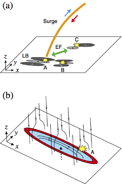
Figure 9: (a) Illustration summarizing activity phenomena in AR 11974. The chromospheric brightenings are found in mixed polarity regions, where the positive field (lighter ellipse with “$+$” sign) and negative field (darker ellipse with “$-$” sign) lie next to each other. Brightening A is located at the light bridge (LB) and ejects dark surges (thick orange line) into the higher atmosphere, which shows a shift from the upward (blue arrow) to downward (red arrow) motion. The light bridge becomes narrower because of the neighboring emerging flux (EF: green arrow). Brightening B has a similar magnetic structure as brightening A. Brightening C is caused by flux cancellation between the positive field sourced from the emerging flux (EF) and the negative polarity. Coordinate system $(x,y,z)$ is consistent with that we used in the analysis of this paper. (b) Schematic illustration of the light bridge. The light bridge shows a broad blue-shifted region (blue) indicating the large-scale upflow from the solar interior (dashed arrow). The upflow carries the horizontal magnetic flux (solid lines with arrows in the bridge), which reconnects with the vertical flux of the surrounding pores (solid lines with arrows outside the bridge) and shows brightening events. One representative event, brightening A, is located in the western edge (denoted as A). The flow drains down in the narrow downflow lane (red).

Figure 9(a) illustrates the general picture that explains the activity phenomena in the analyzed AR. Here, one of the most prominent events is the repeated and intermittent flickering in the chromospheric images. These brightenings are the local heating of chromospheric (or upper-photospheric) plasma via magnetic reconnection and that is why they are seen mainly in the mixed polarity regions. Brightening A occurs in the light bridge, which is the weak, almost horizontal field trapped between the negative pores of almost vertical field. It shows a repeated intensity enhancement with a typical duration of 10–20 minutes. Within each event, it also has a rapid fluctuation with a timescale of 3–5 minutes. Brightening B has a similar magnetic background, while brightening C is caused by the flux cancellation of a pre-existing negative field and a positive field from the emerging flux region. Because of this flux emergence, the negative pores around the light bridge come closer to merge with each other. Eventually the pores form a sunspot, leading to the vanishing of the light bridge.

As well as the local heating, a part of the released energy of magnetic reconnection is converted also into the kinetic energy by launching cool and dense chromospheric plasma into the higher atmosphere in the form of dark surge, which is observed as absorption in EUV images. The surges are recurrently ejected with a typical lifetime of 10–20 minutes, each following the brightening. Due to gravity, the launched cool plasma is pulled back to the surface, showing a parabolic trajectory in the EUV time-slices and a smooth transition from the blueshift to the redshift in the IRIS spectra.

6.2 Light Bridge and its Brightenings

Figure 9(b) shows a schematic illustration of the light bridge. The bridge has a large-scale, long-lasting upflow, which turns into a diverging flow in the horizontal direction. The flow sinks down in the narrow lane at the edge of the bridge. Transported by the large-scale upflow, magnetic flux is continuously provided from the solar interior to the light bridge as a relatively weaker, horizontal field, which is in agreement with previous observations (Beckers & Schröter, 1969; Lites et al., 1991; Rüedi et al., 1995; Leka, 1997; Jurčák et al., 2006). At the same time, the bridge contains small-scale (arcsec-sized) local convection cells with lifetimes of order of 10 minutes. The delivered magnetic flux from the interior has a pattern of 10–15 minutes, probably due to the local convection. As a result, magnetic reconnection takes place repeatedly in the light bridge region between weaker horizontal fields of the light bridge and vertical fields of the surrounding pores with an observed period of 10–20 minutes. The reconnection is seen as the brightenings, while the ejected outflow reaches coronal heights as the dark surges.

One of the brightenings that are observed in this light bridge, namely brightening A, is located at the western end of the bridge. The reason for the repeated brightenings at this location may be that the footpoints of the transported horizontal fields are more likely to be positive in the western part of the bridge, since the observed horizontal fields are mainly eastward (see brightening A in Figure 9(b)). Therefore, as the transported fields pile up at the western end, the magnetic shear between the positive fields within the light bridge and the vertical negative fields of the surrounding pores increases. And thus, the western end becomes a favorable site for the magnetic reconnection, which is observed as series of brightenings.

By comparing the photospheric vertical currents and the chromospheric brightenings in Figure 3, we noticed that the brightenings are located in the middle of the light bridge, while the current sheets are at the edge of the bridge. One possible explanation for this difference is the canopy structure of the magnetic fields above the light bridge (Leka, 1997; Jurčák et al., 2006). Because of the intrusion of the horizontal field of the light bridge, surrounding vertical fields of the pores need to fan out over the bridge until they meet the field lines from the opposite side (see the vertical fields in Figure 9(b)). In the higher altitude, or in the formation layer of the UV lines, the width of the horizontal field region is narrower and more confined to the middle of the bridge. And thus, the UV brightenings are seen in the bridge center, which is deviated from the location of the photospheric current sheet at the both edges. The observed magnitude of the vertical current density, $|j_{z}|\gtrsim 100\ {\rm mA\ m}^{-2}$, is consistent with previously reported values (e.g., Jurčák et al., 2006). Similarly to our observational results, Shimizu et al. (2009) detected the current density higher than $100\ {\rm mA\ m}^{-2}$ along the light bridge. They thought that the strong current was responsible for the intermittent chromospheric jets observed in Ca II H images.

In Figure 3, we found the existence of multiple smaller-sized convection cells in the light bridge, which is consistent with previous observations. Berger & Berdyugina (2003) reported the central dark lanes in the light bridge, indicating the multiple convection cells (see also Sobotka et al., 1994; Hirzberger et al., 2002; Lagg et al., 2014). In our case, small-scale cells had elliptic shapes with elongation along the direction of the light bridge. This may be the consequence of the horizontal field parallel to the light bridge (see review of simulations by Cheung & Isobe, 2014).

6.3 Physical Mechanism of the Dark Surges

The chromospheric brightenings that were repeatedly observed in the UV data were followed by the elongations of dark absorption features in the EUV images, which we call dark surges. Also, the surges were composed of cool, dense (i.e. chromospheric) plasma with a temperature of down to 10,000 K. The observed dark surge shows a very similar behavior to H$\alpha$ surges (Roy, 1973). According to Asai et al. (2001), the ejections from the light bridge in H$\alpha$ and 171 Å images showed that the H$\alpha$ surges are ejected intermittently and recurrently from the light bridge and that the velocities and timings of the 171 Å ejections are the same as those of the H$\alpha$ surges. Roy (1973) reported that all surges observed extend from Ellerman bombs.

What is the physical mechanism that launches the cool chromospheric material into the higher atmosphere from the light bridge? One possible answer is the sling-shot effect of magnetic reconnection. Yokoyama & Shibata (1995, 1996) conducted a numerical simulation of the reconnection between the emerging magnetic field and the pre-existing coronal field. In their model, cool chromospheric plasma is ejected upward by the tension force of curved reconnected field (sling-shot effect), which may be observed as H$\alpha$ surges. Considering the similarities between the H$\alpha$ surges and the dark surges in our analysis, we can speculate that the dark surges are basically produced by the same physical mechanism.

However, it is still difficult to launch such a cool, dense material to the higher altitude. If we assume that the magnetic energy of the light bridge, $B_{\rm LB}^{2}/(8\pi)$, is completely converted into the potential energy of the dark surge, $\rho gH_{\rm DS}$, the height of the surge is given as $H_{\rm DS}=B_{\rm LB}^{2}/(8\pi\rho g)$, where $B_{\rm LB}$, $\rho$, $g$, and $H_{\rm DS}$ are the field strength of the light bridge, the plasma density, the gravitational acceleration, and the height of the dark surge, respectively. If we adopt $B_{\rm LB}\sim 2,000\ {\rm G}$, $\rho\sim 1\times 10^{-8}\ {\rm g\ cm}^{-3}$ (approximate density around the temperature minimum), and $g\sim 2.7\times 10^{4}\ {\rm cm\ s}^{-2}$, then we obtain $H_{\rm DS}\sim 6\ {\rm Mm}$. However, the apparent lengths of the surges in our observation were up to 34 Mm (see Table 1), which indicates that the surge height, $H_{\rm DS}$, is a few 10 Mm. By assuming higher reconnection altitudes and thus applying smaller $\rho$, we may obtain larger $H_{\rm DS}$. However, at the same time, $B_{\rm LB}$ may also become smaller, which may results in insufficient surge heights $H_{\rm DS}$.

One promising idea to overcome this discrepancy is the acceleration by a slow-mode shock (e.g., Shibata et al., 2007). Takasao et al. (2013) conducted numerical simulations similar to those of Yokoyama & Shibata (1996) but of the case that the magnetic reconnection takes place below the transition region, say, in the chromosphere. In such a case, a slow shock is produced and interacts with the transition region. As the transition region is lifted up by the slow shock, the chromospheric plasma extends into much higher altitude. Therefore, the observed dark surge in this study can be launched by the reconnection with the help of slow shock. Moreover, the lifting of the transition region can explain the emission in the front edge of the dark surges seen in some AIA channels, e.g., 304 Å as in Figure 7(a), which are sensitive to the transition region plasma.

7 Conclusion and Outstanding Questions

In this study, we analyzed the light bridge structure in a developing AR and dynamic activity phenomena related to the light bridge, i.e., chromospheric brightenings and dark surges. The observations lead us to conclude that the brightenings and dark surges are driven by magnetoconvective evolution within the light bridge and its interaction with the umbral surroundings. Namely, the convective upflow in the bridge continuously transports the horizontal fields to the surface, which reconnects with adjacent vertical fields, resulting in the repeated and intermittent brightenings and surge ejections. However, we still have some remaining problems.

First of all, the creation of the light bridge structure remains unclear. In the target AR of this study, the light bridge appeared between the two merging pores of the negative polarity. Although the formation process of a light bridge in a mature sunspot was observationally studied in detail by Katsukawa et al. (2007), the light bridge formation in a developing sunspot needs further investigation.

The second issue is the large-scale flow structure in the light bridge. In the present study, the Dopplergrams revealed the existence of a large-scale upflow within the bridge. This upflow transports the magnetic flux from the convection zone to the surface layer and causes magnetic reconnection with the surrounding pore fields, resulting in the production of dynamic events. However, the driver of the large-scale upflow and its transportation mechanism of magnetic flux were not revealed in the present study.

The fine-scale structure of the light bridge is another important topic. For example, the present observation as well as previous observations (e.g., Berger & Berdyugina, 2003) revealed the existence of local convection cells inside the light bridge. However, it is difficult to resolve the such arcsec-sized cells or even subarcsec-sized downflow lanes. Also, it was found that the electric current, $|j_{z}|$, is confined to the narrow boundary layer between the bridge and the external pores. Therefore, revealing the detailed structure of the total current, $|\mbox{\boldmath$j$}|$ instead of $|j_{z}|$, may contribute to better understanding of the occurrence of magnetic reconnection.

These issues will be addressed in Paper II of this series. The first two topics, the formation of the light bridge in a developing AR and its large-scale flow structure, are necessarily linked to the dynamical evolution of an emerging flux region. Also, we need fine-scale and three-dimensional analysis on the bridge structure to reveal the nature of local convection and the structure of total current. Therefore, in Paper II, we will analyze the numerical simulation data of the large-scale three-dimensional flux emergence including thermal convection by Cheung et al. (2010) and investigate the light bridge structure in a spot formation region.

Table 1: Properties of the Dark Surge and Brightening

#		Dark surge				Brightening
		Lifetime	Length	Acceleration		Duration	Max. intensity
		(min)	(Mm)	($10^{4}\ {\rm cm\ s}^{-2}$)		(min)
1		15	11	1.1		25	0.40
2		11	22	4.0		$\arcsec$	$\arcsec$
3		10	8.6	1.9		12	0.31
4		9.0	7.2	2.0		6.8	0.27
5		13	15	2.0		6.8	0.73
6		17	34	2.6		12	0.74
7		23	27	1.1		21	1.0

References

- Asai et al. (2001) Asai, A., Shimojo, M., Isobe, H., et al. 2001, ApJ, 562, L103
- Beckers & Schröter (1969) Beckers, J. M. & Schröter, E. H. 1969, Sol. Phys., 10, 384
- Berger & Berdyugina (2003) Berger, T. E. & Berdyugina, S. V. 2003, ApJ, 589, L117
- Bharti et al. (2007) Bharti, L., Rimmele, T., Jain, R., Jaaffrey, S. N. A., & Smartt, R. N. 2007, MNRAS, 376, 1291
- Bray & Loughhead (1964) Bray, R. J. & Loughhead, R. E. Sunspots, The International Astrophysics Series (London: Chapman & Hall)
- Cheung & Isobe (2014) Cheung, M. C. M. & Isobe, H. 2014, Living Reviews in Solar Physics, 11, 3
- Cheung et al. (2010) Cheung, M. C. M., Rempel, M., Title, A. M., & Schüssler, M. 2010, ApJ, 720, 233
- Choudhuri (1986) Choudhuri, A. R. 1986, ApJ, 302, 809
- De Pontieu et al. (2014) De Pontieu, B., Title, A. M., Lemen, J. R., et al. 2014, Sol. Phys., 289, 2733
- Ellerman (1917) Ellerman, F. 1917, ApJ, 46, 298
- Freeland & Handy (1998) Freeland, S. L. & Handy, B. N. 1998, Sol. Phys., 182, 497
- Garcia de la Rosa (1987) Garcia de La Rosa, J. I. 1987, Sol. Phys., 112, 49
- Hirzberger et al. (2002) Hirzberger, J., Bonet, J. A., Sobotka, M., Vázquez, M., & Hanslmeier, A. 2002, A&A, 383, 275
- Hurlburt et al. (1996) Hurlburt, N. E., Matthews, P. C., & Proctor, M. R. E. 1996, ApJ, 457, 933
- Jurčák et al. (2006) Jurčák, J., Martínez Pillet, V., & Sobotka, M. 2006, A&A, 453, 1079
- Katsukawa et al. (2007) Katsukawa, Y., Yokoyama, T., Berger, T. E., et al. 2007, PASJ, 59S, 577
- Kosugi et al. (2007) Kosugi, T., Matsuzaki, K., Sakao, T., et al. 2007, Sol. Phys., 243, 3
- Lagg et al. (2014) Lagg, A., Solanki, S. K., van Noort, M., & Danilovic, S. 2014, A&A, 568, A60
- Leka (1997) Leka, K. D. 1997, ApJ, 484, 900
- Lemen et al. (2012) Lemen, J. R., Title, A. M., Akin, D. J., et al. 2012, Sol. Phys., 275, 17
- Lites et al. (2013) Lites, B. W., Akin, D. L., Card, G., et al. 2013, Sol. Phys., 283, 579
- Lites et al. (1991) Lites, B. W., Bida, T. A., Johannesson, A., & Scharmer, G. B. 1991, ApJ, 373, 683
- Lites et al. (2007) Lites, B., Casini, R., Garcia, J., & Socas-Navarro, H. 2007, Mem. Soc. Astron. Italiana, 78, 148
- Lites et al. (1995) Lites, B. W., Low, B. C., Martinez Pillet, V., et al. 1995, ApJ, 446, 877
- Louis et al. (2008) Louis, R. E., Bayanna, A. R., Mathew, S. K., & Venkatakrishnan, P. 2008, Sol. Phys., 252, 43
- Louis et al. (2009) Louis, R. E., Bellot Rubio, L. R., Mathew, S. K., & Venkatakrishnan, P. 2009, ApJ, 704, L29
- November & Simon (1988) November, L. J. & Simon, G. W. 1988, ApJ, 333, 427
- Parker (1979) Parker, E. N. 1979, ApJ, 234, 333
- Pereira et al. (2013) Pereira, T. M. D., Leenaarts, J., De Pontieu, B., Carlsson, M., & Uitenbroek, H. 2013, ApJ, 778, 143
- Pesnell et al. (2012) Pesnell, W. D., Thompson, B. J., & Chamberlin, P. C. 2012, Sol. Phys., 275, 3
- Peter et al. (2014) Peter, H., Tian, H., Curdt, W., et al. 2014, Science, 346, 315
- Rempel et al. (2009) Rempel, M., Schüssler, M., & Knölker, M. 2009, ApJ, 691, 640
- Rempel (2011) Rempel, M. 2011, ApJ, 729, 5
- Roy (1973) Roy, J. R. 1973 Sol. Phys., 28, 95
- Rüedi et al. (1995) Rüedi, I., Solanki, S. K., & Livingston, W. 1995, A&A, 302, 543
- Scherrer et al. (2012) Scherrer, P. H., Schou, J., Bush, R. I., et al. 2012, Sol. Phys., 275, 207
- Schou et al. (2012) Schou, J., Scherrer, P. H., Bush, R. I. et al. 2012, Sol. Phys., 275, 229
- Shibata et al. (2007) Shibata, K., Nakamura, T., Matsumoto, T., et al. 2007, Science, 318, 1591
- Shibata & Magara (2011) Shibata, K. & Magara, T. 2011, Living Reviews in Solar Physics, 8, 6
- Shimizu et al. (2009) Shimizu, T., Katsukawa, Y., Kubo, M., et al. 2009, ApJ, 696, L66
- Sobotka et al. (1994) Sobotka, M., Bonet, J. A., & Vazquez, M. 1994, ApJ, 426, 404
- Spruit & Scharmer (2006) Spruit, H. C. & Scharmer, G. B. 2006, A&A, 447, 343
- Takasao et al. (2013) Takasao, S., Isobe, H., & Shibata, K. 2013, PASJ, 65, 62
- Toriumi et al. (2015) Toriumi, S., Cheung, M. C. M., & Katsukawa, Y. 2015, ApJ, in prep
- Toriumi et al. (2014) Toriumi, S., Hayashi, K., & Yokoyama, T. 2014, ApJ, 794, 19
- Tsuneta et al. (2008) Tsuneta, S., Ichimoto, K., Katsukawa, Y., et al. 2008, Sol. Phys., 249, 167
- Vissers et al. (2015) Vissers, G. J. M., Rouppe van der Voort, L. H. M., Rutten, R. J., Carlsson, M., & De Pontieu, B. 2015, submitted to ApJ
- Yokoyama & Shibata (1995) Yokoyama, T. & Shibata, K. 1995, Nature, 375, 42
- Yokoyama & Shibata (1996) Yokoyama, T. & Shibata, K. 1996, PASJ, 48, 353