Engineering Bright Solitons to Enhance the Stability of Two-Component Bose-Einstein Condensates

Abstract

We consider a system of coupled Gross-Pitaevskii (GP) equations describing a binary quasi-one-dimensional Bose-Einstein condensate (BEC) with intrinsic time-dependent attractive interactions, placed in a time-dependent expulsive parabolic potential, in a special case when the system is integrable (a deformed Manakov’s system). Since the nonlinearity in the integrable system which represents binary attractive interactions exponentially decays with time, solitons are also subject to decay. Nevertheless, it is shown that the robustness of bright solitons can be enhanced in this system, making their respective lifetime longer, by matching the time dependence of the interaction strength (adjusted with the help of the Feshbach-resonance management) to the time modulation of the strength of the parabolic potential. The analytical results, and their stability, are corroborated by numerical simulations. In particular, we demonstrate that the addition of random noise does not impact the stability of the solitons.

1 Introduction

The experimental realization of Bose-Einstein condensates (BECs) in dilute gases [1] has provided a deep insight into the realm of macroscopic quantum phenomena, and has now become an experimental testbed for direct manipulations of matter waves. The creation of bright [2] and dark [3] solitons in BEC has drawn additional strong interest to this area [4]. The behavior of the single-component (scalar) BEC is affected by the external trapping potential and the interatomic collisions, characterized by the scattering length. Actually, the lifetime of the self-attractive scalar BEC is very short, as it is subject to decay, once its density exceeds a critical value. Therefore, effective stabilization of self-attractive condensates remains an important problem. In this context, the use of binary (two-component) BECs, composed of either hyperfine states of the same atom [5, 6], or different atomic species [7], may be very relevant, as the dynamics of binary condensates can be controlled by adjusting both the intra- and inter-species scattering lengths via the Feshbach resonance (FR), see book [8] and references therein. In particular, the concept of the exchange of energy between the two components of a binary system, which is known in the realm of optical solitons [9], has been demonstrated in binary condensates as well [10]. This mechanism can be employed to increase the lifetime of the quasi-one-dimensional BEC.

Recently, it was shown [11] that one can manipulate trajectories of bright solitons and their intensity distribution in the coupled nonlinear Schrödinger (NLS) equations by adjusting the respective self-phase-modulation (SPM) and cross-phase modulation (XPM) interactions. Experiments, starting from early works [5], and including more recent ones [6], made use of the repulsive interactions in multi-component BECs composed of ⁸⁷Rb atoms to demonstrate the possibility of producing long-lived multiple-condensate states. Those results, and the availability of multi-component condensates with attractive interactions [12, 13, 14], suggest one to look for a mechanism for enhancing the stability of multi-component BECs by engineering properties of bright solitons, which are coherent condensates by themselves.

In this paper, we consider the dynamics of a binary condensate in an expulsive time-dependent parabolic potential, governed by a system of coupled Gross-Pitaevskii (GP) equations. The motivation to study the properties of the condensates in expulsive potentials stems from the fact that BECs are more stable in the confining trap while they get compressed and are more unstable in the expulsive trap. Expulsive parabolic potentials are also used in experiments for probing various dynamical properties of the condensates [16]. We then study the evolution of the condensates assuming that the scattering length can be made time-dependent through the FR, so as to cast the system into an integrable form. We thus observe that the condensates in the expulsive temporarily transient harmonic potential may sustain stability, while their counterparts in the time-independent potential would rapidly decay. The analytical results are confirmed by numerical simulations employing the split-step Crank-Nicolson method. Furthermore, we demonstrate that the addition of noise does not impact the stability of the condensates in the expulsive transient potential.

2 The model and the Lax pair

Considering a two-component BEC, with equal atomic masses $m$ and attractive interactions (such as the condensate composed of two hyperfine states of ⁷Li [12] or ⁸⁵Rb [14, 15] atoms), trapped in a parabolic potential, the mean-field evolution of the setting is governed by coupled quasi-one-dimensional GP equations [17], written in a scaled form:

$$i\frac{\partial\psi_{1}}{\partial t} = \left(-\frac{1}{2}\frac{\partial^{2}}{\partial x^{2}}+b_{11}|\psi_{1}|^{2}+b_{12}|\psi_{2}|^{2}+\frac{\lambda_{1}^{2}}{2}x^{2}\right)\psi_{1},$$

$$i\frac{\partial\psi_{2}}{\partial t} = \left(-\frac{1}{2}\frac{\partial^{2}}{\partial x^{2}}+b_{21}|\psi_{1}|^{2}+b_{22}|\psi_{2}|^{2}+\frac{\lambda_{2}^{2}}{2}x^{2}\right)\psi_{2},$$ (1)

where $\psi_{j}$ ($j=1,2$) is the macroscopic wave function of the $j$-th component subject to the normalization condition $\int_{-\infty}^{+\infty}|\psi_{1}|^{2}dx=1$ and $\int_{-\infty}^{+\infty}|\psi_{2}|^{2}dx=N_{2}/N_{1}$. The interaction between the atoms is described by the self-interaction coefficients, $b_{jj}=4n_{jj}N_{i}$/$l_{\perp}$, and the interaction between different components is controlled by $b_{jk}=4n_{jk}N_{i}$/$l_{\perp}$, where $n_{jj}$ is the scattering lengths of the $j$-th components, and $n_{jk}$ is the same for collisions between $j$ and $k$ . The dynamics of the two-component BECs composed of hyperfine states of ⁸⁷Rb atoms has been experimentally investigated in detail, and it it was shown how the binary condensates generate various patterns [5, 6]. The system of coupled GP equations for the two-component BEC with unequal scattering lengths is nonintegrable, and has been investigated earlier [18]. In the present work, we consider the condensates with symmetric interaction strengths, [10, 22] assuming $b_{11}=b_{21}=b_{12}=b_{22}$ (the scattering lengths in attractive binary mixtures may be indeed made nearly equal [12, 19, 15]), and $\lambda_{j}^{2}(t)=\omega_{j}^{2}(t)/\omega_{\perp}^{2}$, where $\omega_{j}$ and $\omega_{\perp}$ represent the angular frequencies of the trapping potential in the axial and radial directions, respectively. Time $t$ and coordinate $x$ are measured in units of $2/\omega_{\perp}$ and $l_{\perp}=\sqrt{\hbar/m\omega_{\perp}}$, respectively, while $l_{\perp}$ represents the linear oscillator length of the tight trapping potential acting in the transverse direction.

Further, assuming $\omega_{1}(t)=\omega_{2}(t)=\omega(t)$ (i.e., $\lambda_{1}=\lambda_{2}\equiv\lambda$), and allowing the scattering lengths $b_{jk}$ and the strength of trapping potential $\lambda^{2}$ to vary with time, eq. (1) takes the following form:

$$i\psi_{1t}+\psi_{1xx}+2g(t)(|\psi_{1}|^{2}+|\psi_{2}|^{2})\psi_{1}+\lambda^{2}(t)x^{2}\psi_{1}=0$$

$$i\psi_{2t}+\psi_{2xx}+2g(t)(|\psi_{1}|^{2}+|\psi_{2}|^{2})\psi_{2}+\lambda^{2}(t)x^{2}\psi_{2}=0.$$ (2)

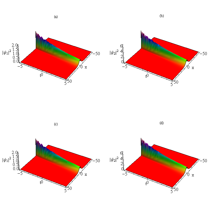
Figure 1: Upper Panels (a-b): The analytical density profile of the bright solitons in the time-independent expulsive trap for $\Gamma=-0.25$ and $g(t)=0.5e^{-0.25t}$. Lower Panels (c-d): The numerically simulated density profile for the same case.

It is relevant to stress, in passing, that we consider the GP equations in the framework of the mean-field approximation, thus completely neglecting quantum correlations which, beyond the limits of the mean-field theory, may cause macroscopic entanglement between matter-wave solitons via their collisions [20, 15, 21].

In eqs. (2), the nonlinearity takes the Manakov’s form [23] (which is a necessary condition if an integrable system is sought for), with $g(t)$ standing for the common interaction strength, while $\lambda(t)$ represents the time-dependent trap frequency. Below, we consider values $g(t)>0$, which correspond to the attractive signs of intraspecies and interspecies interactions. Under the special integrability condition imposed on $g(t)$ and $\lambda(t)$, (see eq. (8) below), eqs. (2) admit a representation in the form of an eigenvalue problem,

$$\Phi_{x} + U\Phi=0,$$

$$\Phi_{t} + V\Phi=0,$$ (3)

where $\Phi=(\phi_{1},\phi_{2},\phi_{3})^{T}$ and

$$U=\left(\begin{array}[]{ccc}i\zeta(t)&Q_{1}&Q_{2}\\ -Q_{1}^{\ast}&-i\zeta(t)&0\\ -Q_{2}^{\ast}&0&-i\zeta(t)\\ &&\end{array}\right),$$ (4)

$$V=\left(\begin{array}[]{ccc}v_{11}&v_{12}&v_{13}\\ v_{21}&v_{22}&v_{23}\\ v_{31}&v_{32}&v_{33}\\ &&\end{array}\right),$$ (5)

with

$$v_{11} = -i\zeta(t)^{2}+i\Gamma(t)x\zeta(t)+\frac{i}{2}Q_{1}Q_{1}^{\ast}+\frac{i}{2}Q_{2}Q_{2}^{\ast}$$

$$v_{12} = \Gamma(t)xQ_{1}-\zeta(t)Q_{1}+\frac{i}{2}Q_{1x}$$

$$v_{13} = \Gamma(t)xQ_{2}-\zeta(t)Q_{2}+\frac{i}{2}Q_{2x}$$

$$v_{21} = -\Gamma(t)xQ_{1}^{\ast}+\zeta(t)Q_{1}^{\ast}+\frac{i}{2}Q_{1x}^{\ast}$$

$$v_{22} = i\zeta(t)^{2}-i\Gamma(t)x\zeta(t)-\frac{i}{2}Q_{1}Q_{1}^{\ast}$$

$$v_{23} = -\frac{i}{2}Q_{2}Q_{1}^{\ast}$$

$$v_{31} = -\Gamma(t)xQ_{2}^{\ast}+\zeta(t)Q_{2}^{\ast}+\frac{i}{2}Q_{2x}^{\ast}$$

$$v_{32} = -\frac{i}{2}Q_{1}Q_{2}^{\ast}$$

$$v_{33} = i\zeta(t)^{2}-i\Gamma(t)x\zeta(t)-\frac{i}{2}Q_{2}Q_{2}^{\ast}$$

$$Q_{1} = \frac{1}{\sqrt{g(t)}}\psi_{1}(x,t)e^{i\Gamma(t)x^{2}/2}$$

$$Q_{2} = \frac{1}{\sqrt{g(t)}}\psi_{2}(x,t)e^{i\Gamma(t)x^{2}/2}$$

The compatibility condition, $(\Phi_{x})_{t}=(\Phi_{t})_{x}$, leads to the zero curvature equation $U_{t}-V_{x}+[U,V]=0$ which yields the integrable system of coupled GP equations (2), provided that the spectral parameter $\zeta(t)$ obeys the following nonisospectral condition:

$$\zeta(t)=\mu\exp\left[-\int\Gamma(t)dt)\right],$$ (6)

where $\mu$ is a hidden complex constant and $\Gamma(t)$ is an arbitrary function of time, which is related to the trapping frequency by the following constraint:

$$\lambda^{2}(t)=\Gamma^{2}(t)-d\Gamma(t)/dt.$$ (7)

Then, it follows from eq. (7) that frequency $\lambda(t)$ is related to scattering length $g(t)$ through the integrability condition:

$$-g(t)d^{2}g(t)/dt^{2}+2\left[dg(t)/dt\right]^{2}-\lambda^{2}(t)g^{2}(t)=0.$$ (8)

Thus, the coupled GP equations (2) is completely integrable if the trapping frequency, $\lambda(t)$, and scattering length, $g(t)$, are subject to constraint (8). For the time-independent trap, $\lambda(t)=\mathrm{const}\equiv c_{1}$, eq. (8) yields $g(t)=e^{c_{1}t}$ [24]. In this work, we focus on the consideration of the integrable system satisfying condition governed by eq. (8). If it is slightly broken, the result depends on the accumulation of the deviation from the integrability over the time interval, $T$, corresponding to essential dynamical regimes, which may be easily identified in all examples displayed below. Namely, if the deviation from the integrability is characterized by difference $\Delta\lambda(t)$ from the value imposed by eq. (8), the condition for the system to remain close to the integrability is

$$\int_{0}^{T}\Delta\lambda(t)dt\ll 1.$$ (9)

It should be mentioned that one can convert the coupled GP equation into the celebrated Manakov’s model by a suitable transformation, as shown, e.g., in ref. [10]. Nevertheless, the direct formulation of the integrability formalism in the form of eqs. (4), (5), and (8) is quite useful, as it makes it possible to apply the gauge-transformation method for generating multisoliton solutions, and it may also be used for the search of more general integrable systems.

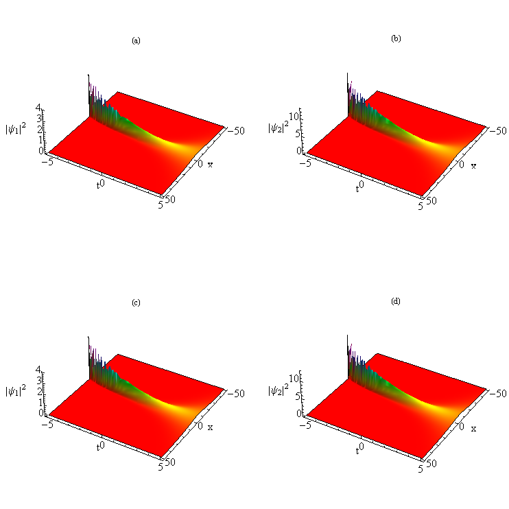
Figure 2: Upper panel (a-b): Analytical results for the compression of the condensate in the time-independent expulsive trap for $\Gamma=-0.5$ and $g(t)=0.5e^{-0.5t}$. Lower Panel (c-d): Numerically simulated density profile for the same case.

3 Analytical and numerical results for two-component bright solitons in the integrable system

Using the gauge-transformation approach [25], bright solitons of the coupled GP equation (2), subject to the integrability condition (8), can be found in the form of

$$\psi_{1}^{(1)} = \sqrt{\frac{1}{g(t)}}\varepsilon_{1}^{(1)}2\beta_{1}(t)\mathrm{sech}(\theta_{1})e^{i(-\xi_{1}+\Gamma(t)x^{2}/2)},$$ (10)

$$\psi_{2}^{(1)} = \sqrt{\frac{1}{g(t)}}\varepsilon_{2}^{(1)}2\beta_{1}(t)\mathrm{sech}(\theta_{1})e^{i(-\xi_{1}+\Gamma(t)x^{2}/2)},$$ (11)

where

$$\theta_{1} = 2\beta_{1}x+4\int\alpha_{1}\beta_{1}dt-2\delta_{1},$$

$$\xi_{1} = 2\alpha_{1}x+2\int(\alpha_{1}^{2}-\beta_{1}^{2})dt-2\chi_{1},$$

with $\alpha_{1}=\alpha_{10}\exp\left[\int{\Gamma(t)}dt\right]$, $\beta_{1}=\beta_{10}\exp\left[\int{\Gamma(t)}dt\right]$ while $\delta_{1}$ and $\chi_{1}$ are arbitrary parameters, and $\varepsilon_{1}^{(1)},\varepsilon_{2}^{(1)}$ are coupling coefficients, which are subject to constraint $|\varepsilon_{1}^{(1)}|^{2}+|\varepsilon_{2}^{(1)}|^{2}=1$. The gauge-transformation approach can be extended to generate multi-soliton solutions [22].

Figure 3: Upper panels (a-b): Onset of the decay (analytical results) for $\Gamma=-0.9$ and $g(t)=0.5e^{-0.9t}$ in the expulsive time-independent trap. Lower Panels (c-d): Numerically simulated density profile for the same case, showing the decay.

Thus, it is obvious from the above that the amplitude of the bright solitons is determined by the temporally modulated scattering length $g(t)$ and trap frequency $\Gamma(t)$ ($\beta_{1}(t)$ varies exponentially with $\Gamma(t)$).

To start the analysis of particular solutions relevant for the physical realization of the system, we now switch off the time dependence of the harmonic trap and adopt the scattering length in the form of $g(t)=0.5e^{-0.25t}$, for which eqs. (7) and (8) render the parabolic potential expulsive, $\Gamma=-0.25$. The corresponding density profile of the condensate is shown in the upper panel of fig. 1 (figs. 1(a) and 1(b)). The corresponding density profile of the condensates produced by numerical simulations of the real time propagation, using the split-step Crank-Nicolson method is shown in figs. 1(c) and 1 (d). From figs. 1(a)-1(d), we observe perfect agreement between the analytical and numerical results. When we double the trapping frequency to $\Gamma=-0.5$, keeping the trap expulsive and choose the scattering length as $g(t)=0.5e^{-0.5t}$ consistent with eqs.(7 ) and (8), the compression of the condensates sets in, as shown in figs. 2(a-b). This is confirmed by numerical simulations shown in figs. 2(c) and 2(d). When we further enhance the trap strength, to $3.6$ times the original value, $\Gamma=-0.9$, keeping the trap expulsive and choose the scattering length as $g(t)=0.5e^{-0.9t}$ (again consistent with the integrability condition given by eqs. (7) and (8)), one observes decay (spreading out) of the condensates, as shown in figs. 3(a-b). Again, results of numerical simulations, shown in figs. 3(c) and 3 (d), match with figs. 3(a) and 3(b), respectively.

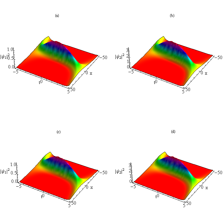
Figure 4: Upper panel (a-b): The analytical density profile produced by switching on the time dependence of the expulsive trap for $\Gamma(t)=-0.25t$ and $g(t)=0.5e^{-0.125t^{2}}$. Lower Panel (c-d): Numerically simulated density profile for $\Gamma(t)=-0.25t$ and $g(t)=0.5e^{-0.125t^{2}}$.

To enhance the stability of the condensates, we now switch ON the time dependence of the harmonic trap, keeping it expulsive, as $\Gamma(t)=-0.25t$, and choose $g(t)=0.5e^{-0.125t^{2}}$, which is consistent with eqs. (7) and (8). The corresponding density profile is shown in figs. 4(a,b). This analytical solution is confirmed by the numerical simulations, as shown in figs. 4(c,d). When we increase the expulsive-potential strength by a factor of $20$ (as compared to fig.(4)), accordingly setting $g(t)=0.5e^{-2.5t^{2}}$, which is consistent with eqs. (7) and (8), the corresponding density profile shown in figs. 5 (a,b) again matches with its numerical counterpart shown in figs. 5(c) and 5(d).

Figure 5: Upper panels (a-b): Analytically found density profiles of the condensates in the time-dependent expulsive potential for $\Gamma(t)=-5t$ and $g(t)=0.5e^{-2.5t^{2}}$. Lower panels (c-d): Numerically found density profiles for the same case.

When we further increase the-time dependent expulsive-trap frequency $\Gamma(t)$ by a factor of $100$ (as compared to fig.(4)), and choose the interaction strength in accordance with eqs.(7) and (8)), an abrupt increase in the density is no more observed, as figs. 6(a-b) show. In fact, any further increase of $\Gamma(t),$ and the respective change of the interaction strength $g(t)$ consistent with eqs. (7) and (8), does not lead to a significant increase in the density, even though the attractive-interaction strength increases rapidly. In other words, the condensates with the attractive interactions in the time-dependent expulsive parabolic potential remain essentially stable over a reasonably large interval of time. Again,analytical results match the numerical simulations, as shown in figs. 6 (c-d).

Figure 6: Upper panels (a-b): The analytically found density profile in the time-dependent expulsive potential for $\Gamma(t)=-25t$ and $g(t)=0.5e^{-12.5t^{2}}$. Lower panels (c-d): The numerically simulated density profile for the same case.

Thus, we observe that the two-component BEC with attractive interactions in the time-dependent expulsive trap, described by the integrable system, is more long-lived, as its lifetime can be increased by means of the FR management, in comparison with the condensates in the time-independent expulsive trap. Note that the scalar (single-component) condensate, stabilized by means of the Feshbach management in a similar setting, quickly decays in the course of the evolution.

To further confirm the stabilization, we added random noise to simulations performed in the time-dependent expulsive trap. The respective numerically simulated density profiles demonstrate, in figs. (7)-(9), that the noise does not impact the stability of the condensates. In all the above numerical simulations, the norm of the wavefunctions is conserved. This conclusion corroborates that the two-component condensate in the time-dependent expulsive harmonic trap, governed by the specially devised integrable system, is more stable in comparison with its counterpart in the time-independent trap. The above results indicate the possibility of increasing the life span of the two-component BEC with attractive interactions in the time-dependent parabolic potential experimentally, employing the FR management, which may be applied to the condensates composed of ³⁹K [13], ⁸⁵Rb [14] and ⁷Li [26] atoms.

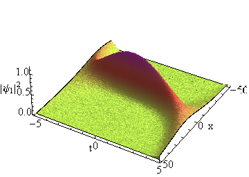
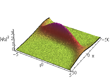
Figure 7: The numerically simulated density profile, corresponding to fig. 4, but withthe addition of random noise.

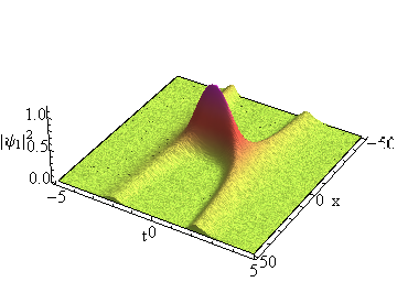
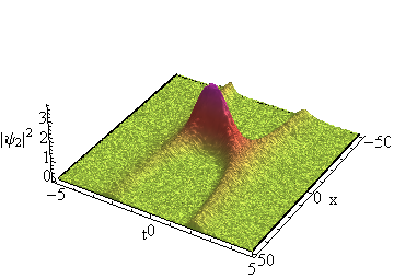
Figure 8: The numerically simulated density profile, corresponding to fig. (5), but with the addition of random noise.

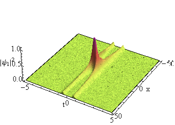
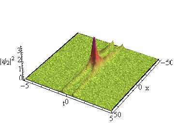
Figure 9: The numerically simulated density profile, corresponding to fig.6 but with the addition of random noise.

4 Conclusion

In this paper, we have shown that one can make use of the precise control of the scattering length by means of the FR (Feshbach resonance) to design conditions under which the mean-field dynamics of two-component condensates in the time-dependent expulsive parabolic potential is governed by the integrable model (a deformation of the Manakov’s system, with a time-dependent scattering length). A regime may be selected, in which solitons stay effectively stable against the decay for a reasonably large interval of time, compared to the condensate in the time-independent expulsive parabolic potential. The analytical results, and their stability, have been corroborated by the comparison with numerical simulations. In particular, it was demonstrated that binary condensate with the attractive interactions remains stable in the time-dependent harmonic potential in spite of the addition of random noise. Thus, the conclusion is that the bright solitons, which would quickly decay (possibly following short-time compression) otherwise, may be made more robust by the proper selection of scattering length through FR management in combination with the appropriate choice of the time dependence of the parabolic potential.

AcknowledgmentsAuthors thank the referees for their suggestions to improve the contents of the paper. PSV and JBS thank University Grants Commission (UGC) and Department of Science and Technology (DST) (India), respectively, for the financial support. RR acknowledges financial assistance received from DST (Ref. No:SR/S2/HEP-26/2012), UGC (Ref. No: F.No 40-420/2011(SR), Department of Atomic Energy -National Board for Higher Mathematics (DAE-NBHM) (Ref.No: NBHM/R.P.16/2014/Fresh dated 22.10.2014) and Council of Scientific and Industrial Research (CSIR) (Ref. No: No.03(1323)/14/EMR-II dated 03.11.2014). This work was supported by the NKBRSFC under grants Nos. 2011CB921502 and 2012CB821305, and NSFC under grants Nos. 61227902 and 61378017.

References

- [1] M. H. Anderson, J. R. Ensher, M. R. Matthews, C. E. Wieman and E. A. Cornell, Science 269 (1995) 198. F. Dalfovo, S. Giorgini, L. P. Pitaevskii and S. Stringari, Rev. Mod. Phys. 71 (1999) 463.
- [2] K. E. Strecker, G. B. Partridge, A. G. Truscott, and R. G. Hulet, Nature 417 (2002) 150. L. Khaykovich, F. Schreck, G. Ferrari, T. Bourdel, J. Cubizolles, L. D. Carr, Y. Castin, and C. Salomon, Science 296 (2002) 1290. K. E. Strecker, G. B. Partridge, A. G. Truscott and R. G. Hulet, New. J. Phys. 5 (2003) 73. S. L. Cornish, S. T. Thompson, and C. E. Wieman, Phys. Rev. Lett. 96 (2006) 170401. A. L. Marchant, T. P. Billam, T. P. Wiles, M. M. H. Yu, S. A. Gardiner and S. L. Cornish, Nature Comm. 4 (2013) 1865. J. H. V. Nguyen, P. Dyke, D. Luo, B. A. Malomed, and R. G. Hulet, Nature Phys. 10 (2014) 918.
- [3] S. Burger, K. Bongs, S. Dettmer, W. Ertmer, K. Sengstock, A. Sanpera, G. V. Shlyapnikov and M. Lewenstein, Phys. Rev. Lett. 83 (1999) 5198. J. Denschlag, J. E. Simsarian, D. L. Feder, C. W. Clark, L. A. Collins, J. Cubizolles, L. Deng, E. W. Hagley, K. Helmerson, W. P. Reinhardt, S. L. Rolston, B. I. Schneider and W. D. Phillips, Science 287 (2000) 97.
- [4] R. Radha, P. S. Vinayagam, Rom. Rep. Phys. 67 No. 1 (2015) 89.
- [5] C. J. Myatt, E. A. Burt, R. W. Ghirst, E. A. Cornell, and C. E. Wieman, Phys. Rev. Lett. 78 (1997) 586. D. S. Hall, M. R. Matthews, J. R. Ensher, C. E. Wieman, and E. A. Cornell, Phys. Rev. Lett. 81 (1998) 1539. D. S. Hall, M. R. Matthews, C. E. Wieman, and E. A. Cornell, Phys. Rev. Lett. 81 (1998) 1543.
- [6] K. M. Mertes, J. W. Merrill, R. Carretero-González, D. J. Frantzeskakis, P. G. Kevrekidis, and D. S. Hall, Phys. Rev. Lett. 99 , 190402 (2007). G. Thalhammer, G. Barontini, L. De Sarlo, J. Catani, F. Minardi, and M. Inguscio, Phys. Rev. Lett. 100 (2008) 210402. S. Tojo, Y. Taguchi, Y. Masuyama, T. Hayashi, H. Saito, and T. Hirano, Phys. Rev. A 82 (2010) 033609. M. A. Hoefer, J. J. Chang, C. Hamner, and P. Engels, Phys. Rev. A 84 (2011), 041605(R).
- [7] G. Thalhammer, G. Barontini, L. De Sarlo, J. Catani1, F. Minardi and M. Inguscio, Phys. Rev. Lett. 100 (2008) 210402.
- [8] B. A. Malomed, Soliton Management in Periodic Systems (Springer: New York, 2006).
- [9] R. Radhakrishnan, M. Lakshmanan and J. Hietarinta, Phys. Rev. E 56 (1997) 2213.
- [10] S. Rajendran, P. Muruganandam and M. Lakshmanan, J. Phys. B: At. Mol. Opt. Phys. 42 (2009) 145307.
- [11] R. Radha, P. S. Vinayagam and K. Porsezian, Phys. Rev. E 88 (2013) 032903.
- [12] E. R. I. Abraham, W. I. McAlexander, J. M. Gerton, R. G. Hulet, R. Côté, and A. Dalgarno, Phys. Rev. A 53 (1996) R3713.
- [13] G. Roati, M. Zaccanti, C. D’Errico, J. Catani, M. Modugno, A. Simoni, M. Inguscio and G. Modugno, Phys. Rev. Lett. 99 (2007) 010403.
- [14] S. L. Cornish, N. R. Claussen, J. L. Roberts, E. A. Cornell and C. E. Wieman, Phys. Rev. Lett. 85 (2000) 1795.
- [15] T. P. Billam, C. L. Blackley, B. Gertjerenken, S. L. Cornish, and C. Weiss, J. Phys.: Conf. Series 497 (2014) 012033.
- [16] L. D. Carr and Y. Castin, Phys. Rev. A 66 (2002) 063602. Z. X. Liang, Z. D. Zhang, and W. M. Liu, Phys. Rev. Lett. 94 (2005) 050402. B. Li, X.-F. Zhang, Y.-Q. Li, Y. Chen, and W.-M. Liu, Phys. Rev. A 78 (2008) 023608.
- [17] C. J. Pethick, H. Smith, Bose-Einstein Condensation in Dilute Gases (Cambridge University Press, Cambridge, 2003) ; L. Pitaevskii and Stringari, Bose Einstein Condensation (Oxford University Press, 2003).
- [18] S. Middelkamp, J. J. Chang, C. Hamner, R. Carretero-González, P. G. Kevrekidis, V. Achilleos, D. J. Frantzeskakis, P. Schmelcher and P. Engels, Phys. Lett. A 375 (2011) 642. E. G. Charalampidis, P. G. Kevrekidis, D. J. Frantzeskakis, and B. A. Malomed, Phys. Rev. E 91 (2015) 012924.
- [19] S. Geltman, J. Phys. B: At. Mol. Opt. Phys. 39 (2006) 4563.
- [20] M. Lewenstein and B. A. Malomed, New J. Phys. 11 (2009) 113014.
- [21] B. Gertjerenken, T. P. Billam, C. L. Blackley, C. Ruth Le Sueur, L. Khaykovich, S. L. Cornish, and C. Weiss, Phys. Rev. Lett. 111 (2013) 100406.
- [22] V. Ramesh Kumar, R. Radha and M. Wadati, Phys. Lett. A 374 (2010) 3685. R.Radha and P. S. Vinayagam, Phys. Lett. A 376 (2012) 944.
- [23] S. V. Manakov, Zh. Eksp. Teor. Fiz. 65 (1973) 505 [Sov. Phys. JETP 38 (1974) 248 ].
- [24] R.Radha and V. Ramesh Kumar Phys. Lett A 370(2007) 46.
- [25] L. -L. Chau, J. C. Shaw, H. C. Yen, J. Math. Phys. 32 (1991) 1737.
- [26] S. E. Pollack, D. Dries, M. Junker,Y. P. Chen, T. A. Corcovilos, and R. G. Hulet, Phys. Rev. Lett. 102 (2009) 090402.