Center Vortices, Area Law and the Catenary Solution

Abstract

We present meson-meson (Wilson loop) correlators in $Z(2)$ center vortex models for the infrared sector of Yang-Mills theory, i.e., a hypercubic lattice model of random vortex surfaces and a continuous 2+1 dimensional model of random vortex lines. In particular we calculate quadratic and circular Wilson loop correlators in the two models respectively and observe that their expectation values follow the area law and show string breaking behavior. Further we calculate the catenary solution for the two cases and try to find indications for minimal surface behavior or string surface tension leading to string constriction.

I Introduction

Many physical principles can be formulated in terms of variational problems. For example the least-action principle is an assertion about the nature of motion that provides an alternative approach to mechanics completely independent of Newton’s laws. Not only does the least-action principle offer a means of formulating classical mechanics that is more flexible and powerful than Newtonian mechanics, but also variations on the least-action principle have proved useful in general relativity theory, quantum field theory, and particle physics. As a result, this principle lies at the core of much of contemporary theoretical physics.

Calculus of variations seeks to find the path, curve, surface, etc., for which a given function has a stationary value, which, in physical problems, is usually a minimum or maximum. In this article we want to use calculus of variations to analyze the (minimal) area law behavior of quark confinement in meson-meson correlators. For this behavior the non-Abelian behavior of the gauge group is essential, and especially the center vortex model of confinement has proved to be very successful in predicting the area law.

Center vortices 'tHooft:1977hy ; Vinciarelli:1978kp ; Yoneya:1978dt ; Cornwall:1979hz ; Mack:1978rq ; Nielsen:1979xu are topological defects associated with the elementary center degree of freedom of the QCD gauge field. In $D$-dimensional space-time, they are (thickened) ($D-2$)-dimensional chromo-magnetic flux degrees of freedom and have a clear theoretical link to confinement 'tHooft:1977hy ; 'tHooft:1979uj ; Greensite:2003bk ; Engelhardt:2004pf . This was confirmed by a multitude of numerical simulations, in lattice Yang-Mills theory, see e.g. DelDebbio:1996mh ; Langfeld:1997jx ; DelDebbio:1997ke ; DelDebbio:1998uu ; Kovacs:1998xm ; Alexandrou:1999iy ; Engelhardt:1999fd ; Bertle:2001xd ; Bertle:2002mm , and within the infrared effective models of center vortices under investigation  Engelhardt:1999wr ; Engelhardt:2003wm ; Altarawneh:2014aa ; Hollwieser:2014lxa . Recent results Greensite:2014gra have also suggested that the center vortex model of confinement is more consistent with lattice results than other currently available models. Lattice QCD simulations indicate further that vortices are responsible for the spontaneous breaking of chiral symmetry ($\chi$SB), dynamical mass generation and the axial $U_{A}(1)$ anomaly deForcrand:1999ms ; Alexandrou:1999vx ; Reinhardt:2000ck2 ; Engelhardt:2002qs ; Leinweber:2006zq ; Bornyakov:2007fz ; Jordan:2007ff ; Hollwieser:2008tq ; Hollwieser:2009wka ; Bowman:2010zr ; Hollwieser:2010mj ; Engelhardt:2010ft ; Hollwieser:2011uj ; Hollwieser:2012kb ; Schweigler:2012ae ; Hollwieser:2013xja ; Trewartha:2014ona ; Brambilla:2014jmp ; Nejad:2015aia ; Trewartha:2015nna , and thus successfully explain the non-perturbative phenomena which characterize the infrared sector of strong interaction physics.

In the present work we measure meson-meson correlators in effective random center vortex models, which will be introduced in the next section. Meson and baryon (Polyakov line) correlators were analyzed in the random vortex world-surface model in Altarawneh:2015bya , showing that the correlators follow an area law behavior. Here we investigate quadratic and circular Wilson (not Polyakov) loop correlators, focusing on the minimal area law. Motivated by the minimal surface of revolution problem we want to analyze possible signs of catenary solutions.

The hanging chain or catenary problem (the world “catenary” comes from the Latin word “catena” meaning chain) was first posed in the Acta Eruditorium in May 1690 by Jacob Bernoulli as follows: ”To find the curve assumed by a loose string hung freely from two fixed points”. Earlier, Galileo mistakenly conjectured that the curve was a parabola. Later Joachim Jung proved that the curve cannot be a parabola but without presenting any solution of the real curve. In June 1691 there were three solutions published, from Leibniz, Huygens and Johann Bernoulli brother of Jacob. Even though these mathematicians approached this problem in three different ways they concluded that the curve was the hyperbolic cosine, which then came to be known as the catenary.

The catenoid is a surface of revolution with minimum area: Any surface of revolution generated by a different curve joining the same endpoints and having the same length, must have a larger surface area. The proof of this fact is less elementary and involves calculus of variations (see e.g. Bliss:1946 ). In section III we derive the so-called catenary solution using the calculus of variations, for both, standard circular and quadratic Wilson loops and compare the results with numerical measurements in section IV. We finish with concluding remarks in V.

II Random center vortex models

Center vortices are expected to behave as random lines (for $D=3$) or random surfaces (for $D=4$). The magnetic flux carried by the vortices is quantized in units which are singled out by the topology of the gauge group, such that the flux is stable against small local fluctuations of the gauge fields. The vortex model of confinement states that the deconfinement transition is simply a percolation transition of these chromo-magnetic flux degrees of freedom. The following infrared effective models in $D=3$ and $D=4$ dimensions have confirmed these expectations and in the latter case also account for topological susceptibility and the (quenched) chiral condensate.

II.1 Random vortex world-line model

In Altarawneh:2014aa ; Hollwieser:2014lxa we introduced a model of random flux lines in $D=2+1$ space-time dimensions. The lines are composed of straight segments connecting nodes randomly distributed in continuous three-dimensional space. Each node is connected to two lines, hence the configuration only consists of closed vortex clusters. The physical space in which the vortex lines are defined is a cuboid $L_{S}^{2}\times L_{T}$ with ”spatial” extent $L_{S}$, ”temporal” extent $L_{T}$ and periodic boundary conditions in all directions. Within this paper we use volumes with $L_{S}=L_{T}=16$, where finite size effects are under control. The vortex length $L$ between two nodes is restricted to a certain range $L_{min}<L<L_{max}$. This range in some sense sets the scale of the model; for practical reasons we choose a scale of $L\approx 1$, i.e. $L_{min}=0.3$ and $L_{max}=1.7$ in these dimensionless units. All updates resulting in vortex lengths $L$ out of the range $L_{min}<L<L_{max}$ are rejected.

An ensemble is generated by Monte Carlo methods, starting with a random initial configuration. Allowance is made for nodes moving as well as being added or deleted from the configurations during Monte Carlo updates. A Metropolis algorithm is applied to all updates using the action $S=\alpha L+\gamma\varphi^{2},$ with action parameters $\alpha=0.11$ and $\gamma=0.33$ for the vortex length $L$ and the vortex angle $\varphi$ between two adjacent segments respectively. The difference of the action of the affected nodes before and after the update determines the probability of the update to be accepted. The move update moves the current node by a random vector of maximal length $r_{m}=4L_{min}$, it affects the action of three nodes, the node itself and its neighbors. The add update adds a node at a random position within a radius $r_{a}=3L_{min}$ around the midpoint between the current and the next node. The action before the update is given by the sum of the action at the current and the next node, while the action after the update is the sum of the action at the current, the new and the next node. Deleting the current node, on the other hand, affects three nodes before the update and only two nodes after the update. Therefore the probability for the add update is in general much smaller than for the delete update and the vortex structure would soon vanish if both updates were tried equally often. Hence, the update strategy is randomized to move a node in two out of three cases ($66\%$), and apply the add update about five times more often than the delete update ($28\%$ vs. $6\%$). A density parameter $d$ is restricting the number of nodes in a certain volume. The add update is rejected if the number of nodes within a $3\times 3\times 3$ volume around the new node exceeds the density parameter $d$.

Furthermore, Monte Carlo updates disconnecting and fusing vortex lines were implemented, i.e., when two vortices approach each other, they can reconnect or separate at a bottleneck. The ensemble therefore will contain not a fixed, but a variable number of closed vortex lines or ”vortex clusters”. Given that the deconfining phase transition is a percolation transition, such processes play a crucial role in the vortex picture. If the current node is not deleted, all nodes around the current node are considered for reconnections. The reconnection update causes the cancellation of two close, nearly parallel vortex lines and reconnection of the involved nodes with new vortex lines. The reconnection update is also subjected to the Metropolis algorithm, considering the action of the four nodes involved.

The model was shown to exhibit both a low-temperature confining phase and a high-temperature deconfined phase, as well as phase transitions with respect to vortex density and segment length $L$. The predictions of the model for the spatial string tension in the deconfined phase quantitatively match corresponding $SU(2)$ lattice Yang-Mills results.

II.2 Random vortex world-surface model

The random vortex world-surface model was introduced in Engelhardt:1999wr ; Engelhardt:2000wc based on the notion that the Yang-Mills vacuum is populated by collective magnetic vortex degrees of freedom which are represented by closed two-dimensional world-surfaces in four-dimensional (Euclidean) space-time. The chromomagnetic flux carried by the vortices is quantized according to the center of the gauge group. The vortex world-surfaces are treated as random surfaces, an ensemble of which in practice is generated using Monte Carlo methods on a hypercubic lattice; the surfaces are composed of elementary squares (plaquettes) on that lattice. The spacing of the lattice is a fixed physical quantity, related to an intrinsic thickness of the vortex fluxes, and represents the ultraviolet cutoff inherent in any infrared effective framework. The action governing the ensemble is related to the surface curvature: If two elementary squares which are part of a vortex surface share a lattice link but do not lie in the same plane, this costs an action increment $c$, where the parameter is set to $c=0.24$, such as to reproduce the $SU(2)$ Yang-Mills ratio of the deconfinement temperature to the square root of the zero-temperature string tension, $T_{C}/\sqrt{\sigma_{0}}=0.69$ Engelhardt:1999wr .

Physically, the random vortex surfaces represent quantized chromomagnetic flux. This means that they contribute in a characteristic way to Wilson loops; if one chooses an area spanning a given Wilson loop - the choice of area is immaterial due to the continuity of flux - then for each time a vortex world-surface pierces that area, the Wilson loop acquires a phase factor corresponding to the center of the gauge group. For the case of $SU(2)$ color treated in this paper, the Wilson loop picks up a $(-1)=\exp(\pm i\pi)$. Note that Wilson loops in the 4D model are defined on a lattice dual to the one on which vortices are defined, i.e. on a lattice shifted by the vector $(a/2,a/2,a/2,a/2)$, where $a$ denotes the lattice spacing. Thus, the notion of a vortex piercing a Wilson loop area is unambiguous.

The vortex ensemble is generated subject to the constraint of continuity of flux (modulo $2\pi$, i.e., modulo Dirac strings Engelhardt:2000wc ; Engelhardt:2002qs ; Engelhardt:2003wm ), forcing thee vortex surfaces to be closed, as already mentioned above. As described in detail in Engelhardt:2003wm , continuity of flux in practice is guaranteed during the generation of the vortex world-surface ensemble by performing updates simultaneously on the six squares making up the surface of an elementary three-dimensional cube in the lattice. This is done in a way which corresponds to superimposing the (continuous) flux of a vortex of the shape of the elementary cube surface onto the flux previously present.

For the $SU(2)$ gauge group, the model was shown to exhibit both a low-temperature confining phase as well as a high-temperature deconfined phase Engelhardt:1999wr , separated by a second-order phase transition Engelhardt:2003wm . The predictions of the model for the spatial string tension in the deconfined phase Engelhardt:1999wr , the topological susceptibility Engelhardt:2000wc and the (quenched) chiral condensate Engelhardt:2002qs quantitatively match corresponding $SU(2)$ lattice Yang-Mills results. Building on this initial progress, the random vortex world-surface model was extended to the case of $SU(3)$ color. Studies of the confinement properties yielded a weakly first-order deconfinement phase transition Engelhardt:2003wm , also seen in the vortex free energy Quandt:2004gy , which represents an alternative order parameter for confinement. Furthermore, a $Y$ law for the baryonic static potential was observed Engelhardt:2004qq and topological susceptibility was studied in Engelhardt:2010ft , which is instrumental in determining, via the $U_{A}(1)$ anomaly, the mass of the $\eta^{\prime}$ meson. Spurred by investigations of Yang-Mills theories with a wider variety of gauge groups, aiming at a better understanding of possible confinement mechanisms Holland:2003kg , the confinement properties of the random vortex world-surface model were subsequently also studied for $SU(4)$ color Engelhardt:2005qu and $Sp(2)$ color Engelhardt:2006ep . These studies showed that the vortex picture can accomodate such diverse color symmetries, while indicating the limitations of the very simple effective dynamics which had proven adequate in the $SU(2)$ and $SU(3)$ cases. Finally, as already mentioned above, meson and baryon correlators were analyzed in the random vortex world-surface model for the latter cases in Altarawneh:2015bya , showing that the correlators follow an area law behavior and are in qualitative agreement with lattice studies.

III The Catenary Solution

A power line hanging between two poles shows us a curve called the catenary. The shape of this natural curve can be derived from a differential equation describing the physics behind a uniform flexible chain hanging by its own weight. The problem was also proposed by W. Symmond in Symmond:1894 in 1894. J. C. Nagel gave a solution in Nagel:1895 that is easy to describe if we accept the reasonable fact that the catenary is the curve with the lowest center of gravity. The problem can be formulated in the same way as minimizing the surface of revolution of a curve between two fixed points, well known from calculus of variation, see e.g. wolfram :

Given $P_{1}$, $P_{2}$ in the plane, find a curve $y(x)$ from $P_{1}$ to $P_{2}$ such that the surface of revolution obtained by revolving the curve about the $x$-axis has minimum surface area. In other words, minimize $2\pi\int_{y(x_{1})}^{y(x_{2})}yds$ with $y(x_{i})=P_{i}$ and $ds$ the line segment along the curve $y(x)$. If $P_{1}$ and $P_{2}$ are not too far apart, relative to $x_{2}-x_{1}$ then the solution is a Catenary (the resulting surface is called a Catenoid), see Fig. 1.

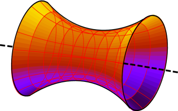
a)             b)

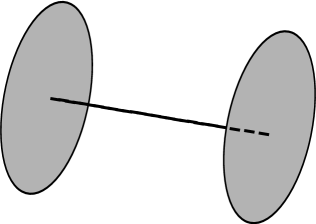
Figure 1: Solutions of the catenary problem for circular Wilson loops: a) Catenoid and b) Goldschmidt’s discontinuous solution.

Otherwise the solution is Goldschmidt’s discontinuous solution (discovered in 1831) obtained by revolving the curve which is the union of three lines: the vertical line from $P_{1}$ to the point $(x_{1},0)$, the vertical line from $P_{2}$ to $(x_{2},0)$ and the segment of the $x$-axis from $(x_{1},0)$ to $(x_{2},0)$. This example also straightforwardly translates to the case of the minimal area law for the Wilson loops, i.e., if the two Wilson loops are far apart, we only measure the product of their expectation values or the string tensions of the two individual meson pairs. However, if the meson pairs approach each other, we measure mixed states all four mesons interact with each other and at some point the strings will flip and form new bound states. The question now is if we can interpret these mixed state measurements with catenary solutions. Therefore we derive the equations for the set of boundary conditions of our problem, starting with the circular Wilson loop.

III.1 Circular Wilson loops

For circular Wilson loops the surface of revolution problem is straightforward. We want to find a curve from a point $(-D/2,R)$ to a point $(D/2,R)$, where $R$ is the radius of the Wilson loop and $D$ is the distance between two Wilson loops, which, when revolved around the $x$-axis yields a surface of smallest surface area $A$, i.e., the minimal surface. The area element is

$$dA=2\pi yds=2\pi y\sqrt{1+y^{\prime 2}}dx,$$ (1)

so the surface area is

$$A=2\pi\int_{-D/2}^{D/2}y\sqrt{1+y^{\prime 2}}dx=4\pi\int_{0}^{D/2}y\sqrt{1+y^{\prime 2}}dx,$$ (2)

and the quantity to minimize is

$$f=y\sqrt{1+y^{\prime 2}}.$$ (3)

This can be solved analytically by using the Beltrami identity, see appendix A, and gives the solution (23)

$$y=a\cosh(\frac{x-b}{a}),$$ (4)

with two constants $a$ and $b$ to be determined from the boundary conditions

$$R=a\cosh(\frac{-D/2-b}{a})=a\cosh(\frac{D/2-b}{a}).$$ (5)

Since $\cosh(-x)=\cosh(x)$ we get $D/2-b=D/2+b$, hence $b=0$, as it must by symmetry, and the minimal surface solution reduces to

$$y=a\cosh(x/a)\quad\mbox{with the boundary condition}\quad R=a\cosh(D/2a),$$ (6)

to determine the constant $a$. But for certain values $R$ and $D$, this equation has no solution. The mathematical interpretation of this fact is that the surface breaks and forms circular disks in each ring to minimize area, i.e. the Goldschmidt solution. Physically it simply means that the minimal area is given by the two Wilson loops rather than any surface of revolution, the two interpretations however do not agree exactly. In appendix B we derive that we only obtain catenary solutions for $D/R<1.325$ (26), but not all solutions are absolute minima of our minimal area problem. The surface area of the minimal catenoid is given by (2)

$$A=4\pi\int_{0}^{D/2}y\sqrt{1+y^{\prime 2}}dx,$$ (7)

but since according to Eqs. (4) and (21)

$$y=a\cosh(x/a)=\sqrt{1+y^{\prime 2}}a,$$ (8)

$$A = \frac{4\pi}{a}\int_{0}^{D/2}y^{2}dx=4\pi a\int_{0}^{D/2}\cosh^{2}(x/a)dx$$ (9)

$$= \pi a^{2}\left[\sinh(\frac{2x}{a})+\frac{2x}{a}\right]_{0}^{D/2}=\pi a^{2}\left[\sinh(D/a)+D/a\right].$$ (10)

The surface area of the catenoid equals that of the Goldschmidt solution when (10) equals the area of two disks, the circular Wilson loops with radius $R$, i.e.,

$$\pi a^{2}\left[\sinh(D/a)+D/a\right] = 2\pi R^{2}$$ (11)

$$\sinh(D/2a)\cosh(D/2a)+D/2a = R^{2}/a^{2}$$ (12)

$$\cosh(D/2a)\sqrt{\cosh^{2}(D/2a)-1}+D/2a = R^{2}/a^{2}.$$ (13)

Defining $u\equiv R/a=\cosh(D/2a)$ from (6) and plugging it in (13) gives $u\sqrt{u^{2}-1}+\cosh^{-1}u=u^{2}$ which has a solution $u\approx 1.211$. The value of $D/R$ for which $A_{catenary}=A_{2disks}$ is therefore $D/R=2\cosh^{-1}u/u\approx 1.055$. For $D/R\in(1.055,1.325)$, the catenary solution has larger area than the two Wilson loops, so it exists only as a local minimum. For $D/R<1.055$ we evaluate the area (10) numerically with $a$ from the boundary condition (6).

III.2 Quadratic Wilson loops

For quadratic Wilson loops the minimal surface solution would probably look like Fig. 2a, i.e., an interpolation of Fig. 2b and the catenary solution in Fig. 1a. We are going to approximate the problem however with the minimal area of Fig. 2b and therefore have to minimize the four lateral surfaces.

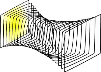
a)             b)

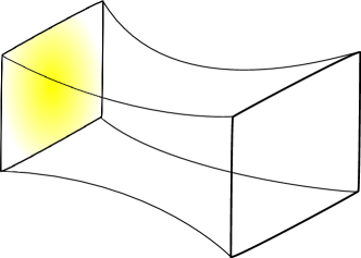
Figure 2: Minimal surface solutions for rectangular Wilson loops.

This can be done by identifying each of the four lateral surfaces with a catenoid, i.e., we unroll the circular solution in Fig. 1a and glue four of them together to obtain the minimal surface solution for rectangular Wilson loops shown in Fig. 2b. Starting from the solution (23) derived in appendix A, we can set the integration constant $b=0$ due to symmetry as above, to obtain

$$y=a\cosh(x/a)\quad\mbox{and}\quad R/2\pi=a\cosh(D/2a),$$ (14)

where the boundary condition is given by the fact that the perimeter of the catenoid circle at $\pm D/2$ (after unrolling) has to be equal to the side length $R$ of the quadratic Wilson loop. This changes the range of possible catenary solutions and yields an upper bound $D/R<0.88$ (27). The total surface is now four times the catenoid (10), i.e.

$$A=4\pi a^{2}\left[\sinh(D/a)+D/a\right],$$ (15)

which equals the Wilson loop areas for $D/R=0.59$, hence we again evaluate the minimal area below this value numerically with $a$ from the boundary condition (14) and compare it to the measurements in the next section.

IV Measurements & Results

We measure meson-meson potentials in the background of random $Z(2)$ center vortex lines or surfaces in $D=3$ and $D=4$ space-time dimensions. In particular, we measure the correlator of two (flat) Wilson loops with circular and quadratic shape, respectively. In fact, these Wilson loops, especially the circular shape, may not represent the perfect observable for measuring meson-meson potentials, as creation and annihilation processes of the quark–anti-quark pairs can not be neglected. But our main interest lies in the comparison with catenary solutions and therefore these shapes are the ideal candidates.

IV.1 Quadratic Wilson loop correlators in the 4D vortex surface model

We measure the correlator of two (flat) Wilson loops of size $R\times R$ at a distance $D$ on $16^{4}$ lattices of random center vortex world-surfaces. The $Z(2)$ vortices contribute a center element $(-1)=\exp(\pm i\pi)$ when they pierce a Wilson loop. The piercing is unambiguous as the vortices live on the dual lattice, as discussed in section II.2. The lattice string tension of the model is $\sigma a^{2}=0.755$ Engelhardt:1999wr gives the scale between (minimal) area and the observable. To reduce the numerical noise contaminating the measurements as far as possible, the exponential noise reduction technique introduced by Lüscher and Weisz Luscher:2001up was employed as introduced in Engelhardt:2004qq for the random center vortex world-surface model. It is a multilevel scheme that exploits the locality of the theory by averaging over sub-ensembles, which can be applied to the random vortex world-surface model as its action (and the Wilson loop) can be decomposed into sub-lattices. In practice, we use the same number of configurations for the individual averaging steps as detailed in Altarawneh:2015bya to achieve the maximum level of accuracy. However, the correlator runs into the double precision regime and breaks down at $-log\langle W(R,R)_{x}W(R,R)_{x+D}\rangle\approx 24$, i.e., for individual Wilson loops $\langle W(R,R)\rangle\approx 10^{-12}$.

We show 3D plots of the measured correlators and the minimal areas determined from the catenary solution (15) or Wilson loop sizes ($2R^{2}$) in Fig. 3 and 2D cuts of the plots vs. $D$ or $R$ in Fig. 5. The data shows perfect area law behavior and we may see agreement with the catenary solution where the coarse lattice data allows the resolution of the effect (Figs. 5b and d at $D=1$ and Fig. 5e at $D=1$ and $2$ resp.) and correspondingly in Figs. 5b and d before the signal is lost in machine precision noise for $R$ and $D>4$.

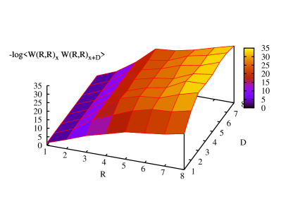
a) b)

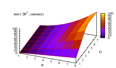
Figure 3: a) $Z(2)$ meson (quadratic Wilson loop) correlators $-log\langle W(R,R)_{x}W(R,R)_{x+D}\rangle$ for various Wilson loop sizes $R$, or distance between quark and anti-quark, and distances $D$ between the meson and anti-meson on $16^{4}$ lattices. b) Surface plot of the minimum of the two Wilson loop areas $2R^{2}$ and the catenoid (15).

IV.2 Circular Wilson loop correlators in the 3D vortex line model

In the continuous model of random center vortex lines we can define circular Wilson loops, hence we measure the correlator of two (flat) Wilson loops of radius $R$ at a distance $D$ in $16^{3}$ volumes with a corresponding string tensions $\sigma a^{2}=0.35$ Altarawneh:2014aa . The Wilson loops again pick a up a factor $(-1)$ when pierced by a vortex line. In this continuous model we can actually go to very small distances where the data precision is still under control, but the catenary effect is also very small. We show 3D plots of the data and the minimal areas determined from the catenary solution (10) or Wilson loop sizes ($2\pi R^{2}$) in Fig. 3 and 2D cuts of the plots vs. $D$ or $R$ in Fig. 7 and Fig. 6 respectively. The results show qualitative agreement with the predicted curves, however they lie significantly below them and can not reveal the small difference between cylinder and catenoid surface areas.

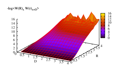
a) b)

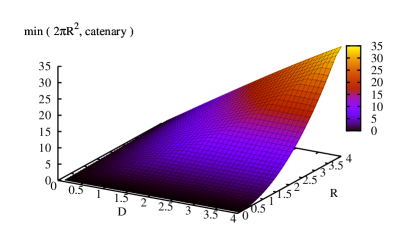
Figure 4: a) Circular Wilson loop correlators $-log\langle W(R)_{x}W(R)_{x+D}\rangle$ for various Wilson loop radii $R$ and distances $D$ between the Wilson loops on $16^{3}$ lattices. b) Surface plot of the minimum of the two Wilson loop areas $2\pi R^{2}$ and the catenoid (10).

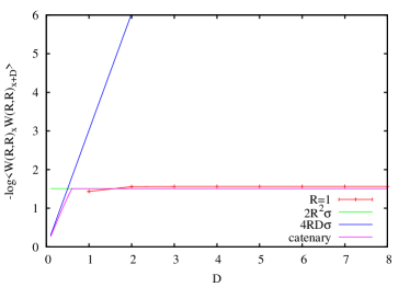
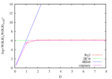
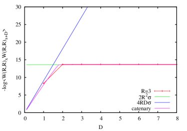
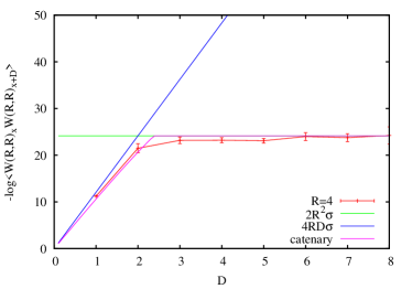
a) b)
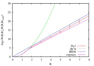
c) d)
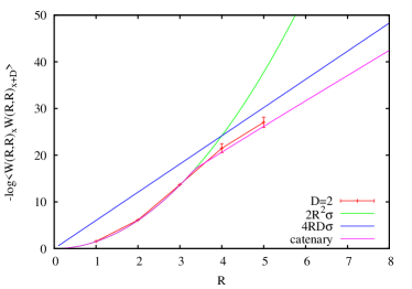
e) f)
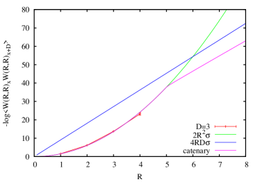
g) h)

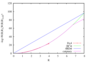
Figure 5: $Z(2)$ meson (quadratic Wilson loop) correlators $-log\langle W(R,R)_{x}W(R,R)_{x+D}\rangle$ versus distance $R$ between quark and anti-quark (Wilson loop size, right column) and distance $D$ between the meson and anti-meson (left column) on $16^{4}$ lattices and minimal area solutions (catenary).

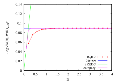
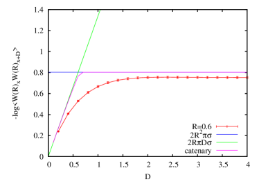
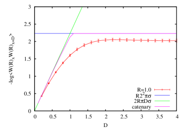
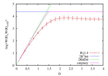
a) b)
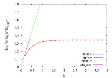
c) d)
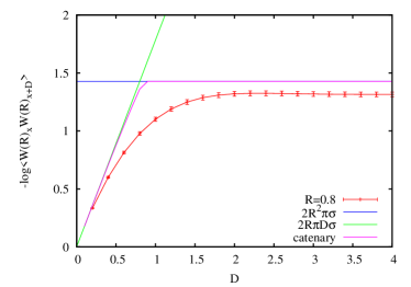
e) f)
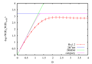
g) h)

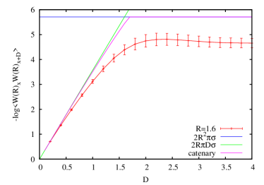
Figure 6: Circular Wilson loop correlators $-log\langle W(R)_{x}W(R)_{x+D}\rangle$ for various Wilson loop radii $R$ versus distance $D$ between the Wilson loops and minimal area solutions.

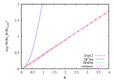
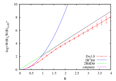
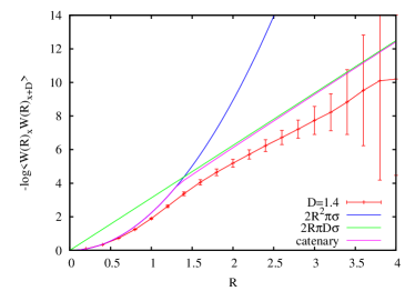
a) b)
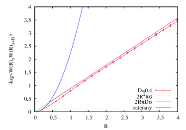
c) d)
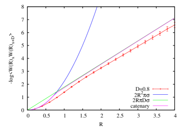
e) f)
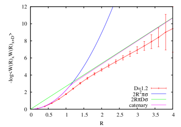
g) h)

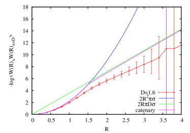
Figure 7: Circular Wilson loop correlators $-log\langle W(R)_{x}W(R)_{x+D}\rangle$ versus Wilson loop radii $R$ for various distances $D$ between the Wilson loops and minimal area solutions.

V Conclusions

We measure quadratic and circular Wilson loop correlators in $Z(2)$ center vortex models for the infrared sector of Yang-Mills theory, i.e., a hypercubic lattice model of random vortex surfaces and a continuous 2+1 dimensional model of random vortex lines. We further calculate the catenary solutions for the Wilson loop configurations and the corresponding catenoid areas. The measurements show minimal area law behavior and may indicate the catenary effects in the hypercubic model, which physically correspond to string surface tension leading to string constriction.

Appendix A Beltrami Identity and Catenary Solution

Starting from the Euler-Lagrange differential equation

$$\frac{\partial f}{\partial y}-\frac{d}{dx}(\frac{\partial f}{\partial y_{x}})=0$$ (16)

we examine the derivative of $f$ with respect to $x$

$$\frac{df}{dx}=\frac{\partial f}{\partial y}y_{x}+\frac{\partial f}{\partial y_{x}}y_{xx}+\frac{\partial f}{\partial x}.$$ (17)

Solving for the $\partial f/\partial y$ term gives

$$\frac{\partial f}{\partial y}y_{x}=\frac{\partial f}{\partial x}-\frac{\partial f}{\partial y_{x}}y_{xx}-\frac{df}{dx}.$$ (18)

Multiplying (16) by $y_{x}$ and substituting the left term with the right hand side of (18) gives

$$\frac{df}{dx}-\frac{\partial f}{\partial y_{x}}y_{xx}-\frac{\partial f}{\partial x}-y_{x}\frac{d}{dx}\frac{\partial f}{\partial y_{x}}=-\frac{\partial f}{\partial x}+\frac{d}{dx}(f-y_{x}\frac{\partial f}{\partial y_{x}})=0.$$ (19)

For $f_{x}=0$ we derive the Beltrami identity with some integration constant $a$,

$$\frac{d}{dx}(f-y_{x}\frac{\partial f}{\partial y_{x}})=0\quad\Rightarrow\quad f-y_{x}\frac{\partial f}{\partial y_{x}}=a,$$ (20)

an identity in calculus of variations discovered in 1868 by Eugenio Beltrami. The quantity $f=y\sqrt{1+y^{\prime 2}}$ from Eq.(3) in section III.1 has in fact $f_{x}=0$, so we can use the Beltrami identity to obtain

$$y\sqrt{1+y^{\prime 2}}-y^{\prime}\frac{yy^{\prime}}{\sqrt{1+y^{\prime 2}}}=a\quad\Rightarrow\quad y(1+y^{\prime 2})-yy^{\prime 2}=y=a\sqrt{1+y^{\prime 2}}$$ (21)

$$y^{\prime 2}=\frac{y^{2}}{a^{2}}-1\quad\Rightarrow\quad y^{\prime}=\frac{\sqrt{y^{2}-a^{2}}}{a}\quad\Rightarrow\quad\frac{dx}{dy}=\frac{1}{y^{\prime}}=\frac{a}{\sqrt{y^{2}-a^{2}}}$$ (22)

$$x=a\int\frac{dy}{\sqrt{y^{2}-a^{2}}}=a\cosh^{-1}(\frac{y}{a})+b\quad\Rightarrow\quad y=a\cosh(\frac{x-b}{a}),$$ (23)

which is called a catenary, and the surface generated by rotating it around the $x$ axis is called a catenoid, see Fig. 1.

Appendix B Catenary vs. Goldschmidt solution

To find the maximum value of $R/D$ at which the catenary solutions (23) resp. (6) for the circular Wilson loop configuration can be obtained, let $p\equiv 1/a$, i.e.,

$$Rp=\cosh(Dp/2).$$ (24)

At the maximum value of $D=D^{*}$ (with corresponding $R^{*}$) it will be true that $dD/dp=0$, hence $d/dp$ of (24) is

$$R^{*}=\sinh(D^{*}p/2)(D^{*}/2+p/2\cdot dD/dp)=D^{*}/2\cdot\sinh(D^{*}p/2).$$ (25)

Dividing (24) at $D^{*}$, i.e., $R^{*}p=\cosh(D^{*}p/2)$ by (25) yields $D^{*}p/2=\coth(D^{*}p/2)$, which has a solution $D^{*}p/2\approx 1.199679$ and from (25) we derive the maximum possible value of

$$D/R\approx 1.32549$$ (26)

for catenary solutions of the circular Wilson loop configuration. For $D/R>1.32549$ only Goldschmidt solutions exist. For the quadratic Wilson loop configuration the corresponding maximum possible value of $D/R$ is given by

$$D/R\approx 0.88013.$$ (27)

- (1) G. ’t Hooft, “On the phase transition towards permanent quark confinement,” Nucl. Phys. B138 (1978) 1.
- (2) P. Vinciarelli, “Fluxon solutions in nonabelian gauge models,” Phys. Lett. B78 (1978) 485–488.
- (3) T. Yoneya, “Z(n) topological excitations in yang-mills theories: Duality and confinement,” Nucl. Phys. B144 (1978) 195.
- (4) J. M. Cornwall, “Quark confinement and Vortices in massive gauge invariant QCD,” Nucl. Phys. B157 (1979) 392.
- (5) G. Mack and V. B. Petkova, “Comparison of Lattice Gauge Theories with gauge groups Z(2) and SU(2),” Ann. Phys. 123 (1979) 442.
- (6) H. B. Nielsen and P. Olesen, “A Quantum Liquid Model for the QCD Vacuum: Gauge and Rotational Invariance of Domained and Quantized Homogeneous Color Fields,” Nucl. Phys. B160 (1979) 380.
- (7) G. ’t Hooft, “A Property of Electric and Magnetic Flux in Nonabelian Gauge Theories,” Nucl.Phys. B153 (1979) 141.
- (8) J. Greensite, “The confinement problem in lattice gauge theory,” Prog. Part. Nucl. Phys. 51 (2003) 1, arXiv:hep-lat/0301023 [hep-lat].
- (9) M. Engelhardt, “Generation of confinement and other nonperturbative effects by infrared gluonic degrees of freedom,” Nucl.Phys.Proc.Suppl. 140 (2005) 92–105, arXiv:hep-lat/0409023 [hep-lat].
- (10) L. Del Debbio, M. Faber, J. Greensite, and Š. Olejník, “Center dominance and Z(2) vortices in SU(2) lattice gauge theory,” Phys. Rev. D 55 (1997) 2298–2306, arXiv:9610005 [hep-lat].
- (11) K. Langfeld, H. Reinhardt, and O. Tennert, “Confinement and scaling of the vortex vacuum of SU(2) lattice gauge theory,” Phys. Lett. B419 (1998) 317–321, arXiv:9710068 [hep-lat].
- (12) L. Del Debbio, and M. Faber, and J. Greensite, and Š. Olejník, “Center dominance, center vortices, and confinement,” arXiv:9708023 [hep-lat].
- (13) L. Del Debbio, M. Faber, J. Giedt, J. Greensite, and Š. Olejník, “Detection of center vortices in the lattice Yang-Mills vacuum,” Phys.Rev. D58 (1998) 094501, arXiv:hep-lat/9801027 [hep-lat].
- (14) T. G. Kovacs and E. T. Tomboulis, “Vortices and confinement at weak coupling,” Phys. Rev. D 57 (1998) 4054–4062, arXiv:9711009 [hep-lat].
- (15) C. Alexandrou, M. D’Elia, and P. de Forcrand, “The Relevance of center vortices,” Nucl.Phys.Proc.Suppl. 83 (2000) 437–439, arXiv:hep-lat/9907028 [hep-lat].
- (16) M. Engelhardt, K. Langfeld, H. Reinhardt, and O. Tennert, “Deconfinement in SU(2) Yang-Mills theory as a center vortex percolation transition,” Phys.Rev. D61 (2000) 054504, arXiv:hep-lat/9904004 [hep-lat].
- (17) R. Bertle, M. Engelhardt, and M. Faber, “Topological susceptibility of Yang-Mills center projection vortices,” Phys. Rev. D 64 (2001) 074504, arXiv:0104004 [hep-lat].
- (18) R. Bertle and M. Faber, “Vortices, confinement and Higgs fields,” arXiv:0212027 [hep-lat].
- (19) M. Engelhardt and H. Reinhardt, “Center vortex model for the infrared sector of Yang-Mills theory: Confinement and deconfinement,” Nucl.Phys. B585 (2000) 591–613, arXiv:hep-lat/9912003 [hep-lat].
- (20) M. Engelhardt, M. Quandt, and H. Reinhardt, “Center vortex model for the infrared sector of SU(3) Yang-Mills theory: Confinement and deconfinement,” Nucl.Phys. B685 (2004) 227–248, arXiv:0311029 [hep-lat].
- (21) D. Altarawneh, M. Engelhardt, and R. Höllwieser, “A model of random center vortex lines in continuous 2+1 dimensional space-time,” (in preparation) (2015) .
- (22) R. Höllwieser, D. Altarawneh, and M. Engelhardt, “Random center vortex lines in continuous 3D space-time,” AIP Conf. Proc. ConfinementXI (2014) to appear, arXiv:1411.7089 [hep-lat].
- (23) J. Greensite and R. Höllwieser, “Double-winding Wilson loops and monopole confinement mechanisms,” Phys. Rev. D91 no. 5, (2015) 054509, arXiv:1411.5091 [hep-lat].
- (24) P. de Forcrand and M. D’Elia, “On the relevance of center vortices to QCD,” Phys. Rev. Lett. 82 (1999) 4582–4585, arXiv:hep-lat/9901020 [hep-lat].
- (25) C. Alexandrou, P. de Forcrand, and M. D’Elia, “The role of center vortices in QCD,” Nucl. Phys. A663 (2000) 1031–1034, arXiv:hep-lat/9909005 [hep-lat].
- (26) H. Reinhardt and M. Engelhardt, “Center vortices in continuum yang-mills theory,” in Quark Confinement and the Hadron Spectrum IV, W. Lucha and K. M. Maung, eds., pp. 150–162. World Scientific, 2002. arXiv:0010031 [hep-th].
- (27) M. Engelhardt, “Center vortex model for the infrared sector of Yang-Mills theory: Quenched Dirac spectrum and chiral condensate,” Nucl.Phys. B638 (2002) 81–110, arXiv:hep-lat/0204002 [hep-lat].
- (28) D. Leinweber, P. Bowman, U. Heller, D. Kusterer, K. Langfeld, et al., “Role of centre vortices in dynamical mass generation,” Nucl.Phys.Proc.Suppl. 161 (2006) 130–135.
- (29) V. Bornyakov et al., “Interrelation between monopoles, vortices, topological charge and chiral symmetry breaking: Analysis using overlap fermions for SU(2),” Phys. Rev. D 77 (2008) 074507, arXiv:0708.3335 [hep-lat].
- (30) G. Jordan, R. Höllwieser, M. Faber, U.M. Heller, “Tests of the lattice index theorem,” Phys. Rev. D 77 (2008) 014515, arXiv:0710.5445 [hep-lat].
- (31) R. Höllwieser, M. Faber, J. Greensite, U.M. Heller, and Š. Olejník, “Center Vortices and the Dirac Spectrum,” Phys. Rev. D 78 (2008) 054508, arXiv:0805.1846 [hep-lat].
- (32) R. Höllwieser, Center vortices and chiral symmetry breaking. PhD thesis, Vienna, Tech. U., Atominst., 2009-01-11. http://katalog.ub.tuwien.ac.at/AC05039934.
- (33) P. O. Bowman, K. Langfeld, D. B. Leinweber, A. Sternbeck, L. von Smekal, et al., “Role of center vortices in chiral symmetry breaking in SU(3) gauge theory,” Phys.Rev. D84 (2011) 034501, arXiv:1010.4624 [hep-lat].
- (34) R. Höllwieser, M. Faber, U.M. Heller, “Lattice Index Theorem and Fractional Topological Charge,” arXiv:1005.1015 [hep-lat].
- (35) M. Engelhardt, “Center vortex model for the infrared sector of SU(3) Yang-Mills theory: Topological susceptibility,” Phys. Rev. D 83 (2011) 025015, arXiv:1008.4953 [hep-lat].
- (36) R. Höllwieser, M. Faber, U.M. Heller, “Intersections of thick Center Vortices, Dirac Eigenmodes and Fractional Topological Charge in SU(2) Lattice Gauge Theory,” JHEP 1106 (2011) 052, arXiv:1103.2669 [hep-lat].
- (37) R. Höllwieser, M. Faber, U.M. Heller, “Critical analysis of topological charge determination in the background of center vortices in SU(2) lattice gauge theory,” Phys. Rev. D 86 (2012) 014513, arXiv:1202.0929 [hep-lat].
- (38) T. Schweigler, R. Höllwieser, M. Faber and U.M. Heller, “Colorful SU(2) center vortices in the continuum and on the lattice,” Phys.Rev. D87 no. 5, (2013) 054504, arXiv:1212.3737 [hep-lat].
- (39) R. Höllwieser, T. Schweigler, M. Faber and U.M. Heller, “Center Vortices and Chiral Symmetry Breaking in SU(2) Lattice Gauge Theory,” Phys.Rev. D88 (2013) 114505, arXiv:1304.1277 [hep-lat].
- (40) D. Trewartha, W. Kamleh, and D. Leinweber, “Centre Vortex Effects on the Overlap Quark Propagator,” PoS LATTICE2014 (2014) 357, arXiv:1411.0766 [hep-lat].
- (41) N. Brambilla, S. Eidelman, P. Foka, S. Gardner, A. Kronfeld, et al., “QCD and Strongly Coupled Gauge Theories: Challenges and Perspectives,” EJPC 74 (2014) Issue 10, arXiv:1404.3723 [hep-ph].
- (42) S.M.H. Nejad, M. Faber and R. Höllwieser, “Colorful plane vortices and Chiral Symmetry Breaking in Lattice Gauge Theory,” arXiv:1508.01042 [hep-lat].
- (43) D. Trewartha, W. Kamleh, and D. Leinweber, “Evidence that centre vortices underpin dynamical chiral symmetry breaking in SU(3) gauge theory,” Phys. Lett. B747 (2015) 373–377, arXiv:1502.06753 [hep-lat].
- (44) D. Altarawneh, R. Höllwieser and M. Engelhardt, “Confining bond rearrangement in random center vortex models,” (submitted to JHEP) (2015) , arXiv:1508.07596 [hep-lat].
- (45) G. A. Bliss, “Lectures on the calculus of variations,” Univ. Chicago Press, Chicago, Ill. (1946) .
- (46) M. Engelhardt, “Center vortex model for the infrared sector of Yang-Mills theory: Topological susceptibility,” Nucl.Phys. B585 (2000) 614, arXiv:0004013 [hep-lat].
- (47) M. Quandt, H. Reinhardt, and M. Engelhardt, “Center vortex model for the infrared sector of SU(3) Yang-Mills theory - vortex free energy,” Phys.Rev. D71 (2005) 054026, arXiv:hep-lat/0412033 [hep-lat].
- (48) M. Engelhardt, “Center vortex model for the infrared sector of SU(3) Yang-Mills theory - baryonic potential,” Phys. Rev. D 70 (2004) 074004, arXiv:0406022 [hep-lat].
- (49) K. Holland, M. Pepe, and U. Wiese, “The Deconfinement phase transition of Sp(2) and Sp(3) Yang-Mills theories in (2+1)-dimensions and (3+1)-dimensions,” Nucl.Phys. B694 (2004) 35–58, arXiv:hep-lat/0312022 [hep-lat].
- (50) M. Engelhardt, “Center vortex model for the infrared sector of SU(4) Yang-Mills theory: String tensions and deconfinement transition,” Phys. Rev. D 73 (2006) 034015, arXiv:0512015 [hep-lat].
- (51) M. Engelhardt and B. Sperisen, “Center vortex model for Sp(2) Yang-Mills theory,” Phys.Rev. D74 (2006) 125011, arXiv:hep-lat/0610074 [hep-lat].
- (52) W. Symmond, “Problem 33,” Amer. Math. Monthly 1 (1894) 437–438.
- (53) J. C. Nagel, “Solution to prob. 33,” Amer. Math. Monthly 2 (1895) 193.
- (54) http://mathworld.wolfram.com.
- (55) M. Lüscher and P. Weisz, “Locality and exponential error reduction in numerical lattice gauge theory,” JHEP 0109 (2001) 010, arXiv:hep-lat/0108014 [hep-lat].