Dynamic Network Formation with Foresighted Agents

Abstract

What networks can form and persist when agents are self-interested? Can such networks be efficient? A substantial theoretical literature predicts that the only networks that can form and persist must have very special shapes and that such networks cannot be efficient, but these predictions are in stark contrast to empirical findings. In this paper, we present a new model of network formation. In contrast to the existing literature, our model is dynamic (rather than static), we model agents as foresighted (rather than myopic) and we allow for the possibility that agents are heterogeneous (rather than homogeneous). We show that a very wide variety of networks can form and persist; in particular, efficient networks can form and persist if they provide every agent a strictly positive payoff. For the widely-studied connections model, we provide a full characterization of the set of efficient networks that can form and persist. Our predictions are consistent with empirical findings.

Keywords: Network formation, Foresight, Heterogeneity, Incomplete Information, Efficiency

JEL Classification: A14, C72, D62, D83, D85

1 Introduction

Much of society is organized in networks and networks are important because individuals typically interact largely or perhaps entirely with those to whom they are closest in the network (not necessarily physically). Examples include social networks (Facebook), professional networks (LinkedIn), trading networks (Tesfatsion[32]), channels of information sharing (Chamley and Gale[3]), buyer-seller networks (Kranton and Minehart[22]), etc. The questions which this paper addresses are: What networks form and emerge at equilibrium if agents are foresighted? Are these networks efficient? Are the emerging networks robust to various types of deviations?

Network formation has been widely studied both in theoretical and empirical settings. Starting from Jackson and Wolinsky[18] and Bala and Goyal[1], a large and growing theoretical literature in economics has studied what networks form when self-interested and strategic agents make decisions about which links to establish or sever with other agents. Past research has mainly focused on characterizing the networks emerging at equilibrium and determining whether socially-efficient networks can be supported in equilibrium.

In the existing literature, network formation has been either modeled in a static setting (e.g. Jackson and Wolinsky[18]), where agents take actions only once and simultaneously, or a dynamic setting (e.g. Watts[33]) where agents meet other agents randomly over time and choose their actions (on whether to form or break a link with another agent) whenever they are allowed to do so. Both these model have two important limitations: i) agents are myopic, i.e. their actions at any point in time are solely guided by their current payoffs, without consideration of future consequences; and ii) agents are homogeneous, i.e. an agent’s payoff depends only on the network topology and her position in the network, but not on her own characteristics or the characteristics of her peers. Such limitations make this literature unable to model and characterize real-world social and economic interactions. One of the key conclusions of this branch of literature is that efficiency cannot be attained in equilibrium and the set of achievable network topologies and that of efficient network topologies often differ. The existing limited work on network formation with foresighted agents (see for example Dutta et al.[6]) shares this negative result: they show that there are various valuation structures in which no equilibrium can sustain efficient network topologies. These findings are in stark contrast to empirical findings which suggest that efficient network topologies often emerge in practice.

In this paper, we provide a first model and comprehensive analysis of dynamic network formation that does not suffer from the abovementioned limitations. We adopt a standard dynamic network formation game, where agents meet one another randomly at discrete times, and they choose whether to form or break links with other agents. As it is standard in the network formation literature, we assume that link formation requires bilateral consent while link severance is unilateral. We relax two key limitations of the existing work. In our model, agents are heterogeneous, i.e. their payoffs depend on their own characteristics and the characteristics of their peers as well as the topology of the network and their position in the network. More importantly, agents are foresighted: in making decisions they take into account both the current consequences of their decisions and the future consequences of these decisions. Foresight plays an important role in virtually all environments and would seem to play an especially important role in network formation: agents may incur substantial costs to form or maintain links that yield small current benefits because they (correctly) foresee that forming these links will encourage linking behavior of others in a way that yields large future benefits. Analysis that ignores the effects of foresightedness (and treats behavior as myopic) misses an important piece of agents’ cost-benefit analysis. With hindsight, it is perhaps not surprising that such analysis – while simpler than the analysis carried out here – leads to predictions that are less consistent with empirical observations of real-life networks.

The dynamic game we analyze is a stochastic game in which states are determined by the random selection process as well as the agents’ actions. When types are private knowledge, this game is also a Bayesian game, in which agents learn dynamically and update their beliefs based on observation of the formation history. As is common in the literature on dynamic games, our focus is characterizing the equilibrium behavior and outcomes when agents are patient. However, instead of characterizing the set of achievable payoffs as in the repeated-game literature, we aim to characterize the set of networks which persist (do not change) in equillibrium (forever).

Our main findings are presented in three theorems. Theorem 1 is a Network Convergence Theorem for the setting where agents have complete information about characteristics of others. It demonstrates that networks that yield each agent a positive one-period payoff can persist in the long-run. The equilibrium strategies we construct are Markov, and robust in several dimensions: to initial configurations, to agent trembles, and to group deviations.

For a widely studied special case of our model, the connections model, our results are directly comparable to previous theoretical and empirical work, especially with respect to the sustainability of efficient networks. Theorem 2 extends the setting of Jackson and Wolinsky[18] to heterogeneous agents who act foresightedly. This extension yields predictions that are much more consistent with empirical findings than previous work. In particular, we predict that efficient networks may be obtained in equilibrium, in contrast to [18] which predicts that efficient networks almost never obtain. (See below for further discussion.)

Theorem 3 is a Network Convergence Theorem for the setting in which information is incomplete: agents begin with prior beliefs about the characteristics of others and perform Bayesian updates based on observed history. Under natural assumptions about the valuation structure, there exists an equilibrium in which patient agents are incentivized to reveal their types by making connections. In such an equilibrium, information becomes ultimately complete and again, any network yielding a positive one-period payoff for every agent can be sustained. This result points to a tractable equilibrium strategy profile that covers the range of sustainable network topologies and involves a simple updating process.

In summary, our results yield a new and positive basis for the sustainability of efficiency in networks: in settings in which efficient networks provide every agent with a positive payoff, these networks can be sustained in equilibrium as long as agents are patients. This is true for both the complete and incomplete information case. Nevertheless, we find that in typical cases the agents need to be more patient under incomplete information than under complete information to achieve efficiency.

The remainder of the paper is organized as follows: Section 2 provides a review of the related literature. Section 3 introduces the model. Section 4 presents the Network Convergence Theorem under complete information on types, with an explicit construction of equilibrium strategies and a discussion on robustness. Section 5 analyzes the connections model and characterizes the generically unique efficient network topology. Section 6 introduces the Network Convergence Theorem under incomplete information and illustrates the contrast between complete and incomplete information. Section 7 concludes the paper.

2 Literature Review

The existing economics literature on network formation can be generally categorized in two main classes: settings in which the agents link formation is bilateral or unilateral, i.e. whether the creation of a link requires bilateral consent of both agents involved, or can be done unilaterally by an agent. Numerous social networks applications such as Facebook, Google+ etc. are best modeled using models appertaining to the first category, while Twitter is best modeled in the second category. The well-known connections model by Jackson and Wolinsky[18] falls into the first category as do the models considered in this paper. Considering static strategic environment with homogeneous and myopic agents, [18] argued that strongly efficient networks are necessarily either empty or a star or a clique and that in generic cases strongly efficient networks cannot be sustained via agents’ self-interested behavior. In the second category, Bala and Goyal[1] provided a comprehensive analysis which yields quite different predictions on the efficient network topologies and the equilibrium network topologies. However, we will not elaborate on their results in this paper since our models falls into the first category.

A more recent development in static network formation is to introduce heterogeneity among agents. Heterogeneity takes different forms in different branches in the literature, but it can be divided into two main categories. The first type of heterogeneity is exogenous, such as different failure probabilities for different links (Haller and Sarangi[15]) and agent-specific values and costs (Galeotti[10], Galeotti et al.[12]). The second type is endogenous heterogeneity, often represented as the amount of valuable resource produced by the agents themselves, as in Galeotti and Goyal[11]. In our paper, we adopt the first approach since the heterogeneity we focus on is an agent’s endowed individual characteristic. We assume a more general framework than most existing literature by assigning each agent a type that may affect others’ payoffs as well as her own. We conduct our analysis in both cases where types are common knowledge (complete information) and where they are private knowledge (incomplete information).

Another strand of literature describes network formation as an interactive process over time, instead of a one-shot, static action profile. Again, various methods have been proposed. For instance, Johnson and Gilles[19] and Deroian[5] analyze variations of the connections model in a finite sequential game, and Konig et al.[20] models network formation as a continuous-time Markov chain with random arrival of link creation opportunities. In this paper, we follow the network formation game introduced by Watts[33], in which pairs of agents are selected randomly on a discrete and infinite time line to update the potential link between them. A link is formed or maintained with bilateral consent, and not formed or severed if either agent chooses to do so. This framework and variations of it have been widely adopted to analyze strategic interactions in social and economic networks (Jackson and Watts[17], Skyrms and Pemantle[30], Song and van der Schaar[31]).

In works adopting this dynamic model, agent myopia is a common assumption, which means that agents only take into account their current payoffs at every point of decision; another prevalent assumption is agent homogeneity, with the exception of our prior work in [31], where we analyzed a variation of the connections model where an agent’s payoff is affected by others’ types but not his own. In terms of sustaining efficient networks, predictions made are similar to Jackson and Wolinsky [18]: the strongly efficient network cannot be sustained at all times in the formation process. The formation and persistence of the strongly efficient network is random – it depends on the realized selection of agent pairs in the early state – and as a result the probability of sustaining the efficient network decreases as the number of agents increases.

There have been a few attempts to introduce foresightedness into the dynamic network formation, but overall this topic remains understudied. This paper is related to Dutta et al.[6], who also adopted the model of Watts[33] and assumed that agents take future payoffs into account. Their main result once again points to the impossibility of sustaining efficient networks in equilibrium by constructing a representative example. The major difference between our paper and this paper is that we allow for a public signal in the definition of a state in a Markov strategy profile – in this way, the agents may have only limited knowledge about the past formation history but will still be able to cooperate in achieving efficiency. Our positive result on sustaining efficient networks holds for a more general valuation structure than most existing frameworks. Alternative models on foresightedness in network formation include Page Jr. et al.[28] and Herings et al.[16], whose solution concept is a pairwise stable network instead of equilibrium. Yet again the efficiency-related results point to cases where the strongly efficient network cannot be sustained even if it provides each player a positive payoff.

Our approach to the analysis and in particular our construction of equilibrium strategies owes a great deal to the work of Dutta[7] and Forges[9]. In particular, we share the general notion of characterizing patient agents’ behavior (though in the sense of network topologies formed instead of payoffs attained) and our construction of equilibrium strategy profiles benefit from the existence of a “uniform punishment strategy” mentioned in Forges[9].

There are numerous empirical studies characterizing the properties of real-world networks. The major properties identified by these works are: short diameter (Albert and Barabasi[2]), high clustering (Watts and Strogatz[34]), positive assortativity (Newman[26][27]), and inverse relation between clustering coefficient and degree (Goyal et al.[14]). Moreover, experimental studies such as Falk and Kosfeld[8], Corbae and Duffy[4], Goeree et al.[13] and Rong and Houser[29] have indicated that typical equilibrium network topologies predicted by the existing theoretical analysis, especially the star network, only emerge in a small fraction of experimental outcomes. Last but not least, Mele[25] and Leung[24] show that networks formed in large social communities, where agents are heterogeneous and withhold certain private information, often exhibit patterns not predicted by existing theoretical literature. In the subsequent analysis, we will discuss most of the above properties and illustrate how they can be accounted for in our framework.

3 Model

3.1 Network Topology

Consider a group of agents $I=\{1,2,...,N\}$. We consider undirected networks. Thus, a network is a collection of unordered pairs of distinct elements of I: ${\bf{g}}\subset\mathcal{{G}}(I)=\{ij:i,j\in I,i\neq j\}$. $ij$ is called a link between agents $i$ and $j$. A network ${\bf{g}}$ is empty if ${\bf{g}}=\varnothing$. (Agents who are not linked to anyone are singletons; in the empty network, all agents are singletons.) Let $G(I)=2^{\mathcal{{G}}(I)}$ denote the set of all possible networks. Given a subset of agents $I^{\prime}$, let $G_{I^{\prime}}$ denote a network that is formed within $I^{\prime}$.

Given a network ${\bf{g}}$ we say that agents $i$ and $j$ are connected, denoted $i\overset{{\bf{g}}}{\leftrightarrow}j$, if there exist $j_{1},j_{2},...,j_{n}$ for some $n$ such that $ij_{1},j_{1}j_{2},...,j_{n}j\in{\bf{g}}$. Let $d_{ij}$ denote the distance, or the smallest number of links between $i$ and $j$. If $i$ and $j$ are not connected, define $d_{ij}:=\infty$.

Let $N({\bf{g}})=\{i|\exists j\text{ s.t. }ij\in{\bf{g}}\}$ be the set of non-singletons, and let $N_{i}({\bf{g}})=\{j:ij\in{\bf{g}}\}$ be the set of neighbors of i. A component of network ${\bf{g}}$ is a maximal connected sub-network, i.e. a set $C\subset{\bf{g}}$ such that for all $i\in N(C)$ and $j\in N(C)$, $i\neq j$, we have $i\overset{C}{\leftrightarrow}j$, and for all $i\in N(C)$ and $j\in N({\bf{g}})$, $ij\in{\bf{g}}$ implies that $ij\in C$. Let $C_{i}$ denote the component that contains link $ij$ for some $j\neq i$. Unless otherwise specified, in the remaining parts of the paper we use the word “component” to refer to any non-empty component.

A network ${\bf{g}}$ is said to be empty if ${\bf{g}}=\varnothing$, and connected if ${\bf{g}}$ has only one component which is itself. ${\bf{g}}$ is minimal if for every component $C\subset{\bf{g}}$ and every link $ij\in C$, the absence of $ij$ would disconnect at least one pair of formerly connected agents. ${\bf{g}}$ is minimally connected if it is minimal and connected.

3.2 Dynamic Network Formation Game

We adopt the framework by Watts[33] to formulate the network formation game. Time is discrete and the horizon is infinite: $t=1,2,...$. We assume an initial network ${\bf{g}}(0)$; this is a parameter. The game is played as follows:

• 1. In each period, a pair of agents $(i,j)$ is randomly selected with equal probabilities to update the link between them.

• 2. The two selected agents (each knowing the identity of the other) then play a simultaneous move game: if there is a link between them, each can choose to sever the link or not; if there is no link between them, each can choose to form a link or not. An existing link can be severed unilaterally, whereas formation of a link requires mutual consent.

• 3. In addition, in each period every agent (whether or not she is selected in the current period) can choose to sever any of her existing links.

It is convenient not to distinguish between severing a link and not forming a link. Hence, for each agent i and each agent j, i has two possible actions with respect to j: $a_{ij}=1$ denotes the action that $i$ agrees to form a link with $j$ (if there is no existing link) or not to sever the link (if there is an existing one), and $a_{ij}=0$ otherwise. We emphasize that a link is formed or maintained after bilateral consent (i.e. $a_{ij}=a_{ji}=1$). Write $\mathcal{A}=\{0,1\}$.

Let $\phi(t)$ be the pair of agents selected in period $t$ and let $\sigma(t):=\{\phi(\tau),{\bf{g}}(\tau)\}_{\tau=1}^{t}$ denote a formation history or a formation path up to time $t$, with the initial condition that $\sigma(0)=(\varnothing,\varnothing)$. Let $\Sigma=\{\sigma(t):t\in\mathbb{N}\}$ denote the set of all possible formation histories. It is important to note that the formation history is different from the sequence of actions taken in two aspects. Conceptually, the formation history is a record of the evolution of the network from an outsider’s point of view. In other words, it is the set of all possible public information, whereas the actions are part of the agents’ private information. Technically, even though the formation history is determined by actions taken over time, it does not perfectly reveal every action. For instance, seeing a link broken or not formed in the formation history only implies that at least one of the two related agents chose action 0 in that period, but it does not identify the agent(s) who did so.

Agents may not observe the entire formation history, but in each period every agent $i$ knows its neighbors $N_{i}({\bf{g}})$, i.e. the set of agents she links to. In addition, in each period the agents observe a public signal which is generated by a signal device $y:\Sigma\rightarrow Y$, where $Y$ is the set of signal realizations. We sometimes refer to $y$ as the monitoring structure in the remainder of this paper. In general, the signal generated may depend on the entire formation history and not only on the current actions. (Of course, the latter is a special case.) We assume that $y$ and $Y$ are common knowledge.

The signal device determines what agents know about the formation history. For instance, if $Y=\{0\}$ and $y(\sigma(t))=0$ then agents have no knowledge of the formation history whatsoever; if $Y=\Sigma$ and $y(\sigma(t))=\sigma(t)$ then agents have complete knowledge of the formation history. If agents observe the events of each period, i.e. $(\phi(\tau),{\bf{g}}(\tau))$ for each $\tau$, then they implicitly observe the full history $\sigma(t)$. In general however, some incomplete monitoring structure cannot be generated by single period reports; see our discussion in Section 5. Intermediate signals structures represent incomplete observability. Note however, that $y$ is deterministic instead of random, so our notion of incomplete observability is different from the perhaps more familar notion of imperfect monitoring.

In the various applications of this model, especially social networks, the signal device can be interpreted as a news media, e.g. a newspaper, a television program or a website. It will not record everything in the past for its audience, but it broadcasts important events that attract public attention or irregular or inappropriate activities by certain individuals. As we will see even incomplete knowledge about the formation history is sufficient to sustain efficient networks in equilibrium.

3.3 Payoff Structure

Each agent has a type, denoted by $\theta_{i}$ for agent $i$. Let $\Theta\subset\mathbb{R}$ denote the set of possible types. Let $\bar{\theta}=(\theta_{1},\theta_{2},\cdots)$ denote the type vector for the whole group of agents. Given a subset of agents $I^{\prime}$, let $\bar{\theta}_{I^{\prime}}$ denote the associated type vector.

The one-period payoff of agent $i$ depends on the network structure and the type vector. Specifically, this payoff is a function $u_{i}:\Theta^{N}\times G(I)\rightarrow\mathbb{R}$. We assume that the payoff to agent $i$ is zero whenever agent $i$ is a singleton: $u_{i}(\bar{\theta},{\bf{g}})=0$ for all ${\bf{g}}$ in which $i$ is a singleton, regardless of $\bar{\theta}$ and ${\bf{g}}$. Also, we assume that each agent’s payoff satisfies component independence: $u_{i}(\bar{\theta},{\bf{g}})=u_{i}(\bar{\theta},C_{i})$.

For each agent, her payoff is realized in every period, though payoffs in different periods may well be different according to the network topology. A payoff that realizes $t$ periods from now is discounted by $\gamma^{t}$, where $\gamma\in(0,1)$ is the time discount factor. Hence, if the vector of networks that form over time is $\bar{g}=\{{\bf{g}}(\tau)\}_{\tau=1}^{\infty}$, agent $i$’s total (discounted) payoff evaluated at period $t$ is

$$U_{i}(\bar{\theta},\bar{{\bf{g}}},t)=\sum_{\tau=0}^{\infty}\gamma^{\tau}u_{i}(\bar{\theta},{\bf{g}}(t+\tau)).$$

If the network is constant from time $t$ onward, this reduces to $(1-\gamma)^{-1}u_{i}(\bar{\theta},{\bf{g}}(t))$.

In our analysis, we will discuss the possibility of converging to an efficient network structure. Following the convention in the literature, our benchmark for efficiency will be the strongly efficient network, i.e. the network that yields the largest sum of one-period payoffs. We provide a formal definition below.

Definition 1 (Strong efficiency).

Given $\bar{\theta}$, a network ${\bf{g}}$ is strongly efficient if $\sum_{i=1}^{N}u_{i}(\bar{\theta},{\bf{g}})\geq\sum_{i=1}^{N}u_{i}(\bar{\theta},{\bf{g}}^{\prime})$ for every ${\bf{g}}^{\prime}$.

Since the number of possible network topologies is finite, a strongly efficient network always exists.

Another type of network we identify is a core-stable network. In a later section we will demonstrate that such a network entails important additional properties of the formation process.

Definition 2 (Core-Stable network).

A network ${\bf{g}}$ is core-stable if there exists no subgroup of agents $I^{\prime}\subset I$ and network ${\bf{g}}^{\prime}$ among $I^{\prime}$ (that is, there is no link $ij\in{\bf{g}^{\prime}}$ with $i\in I^{\prime}$ and $j\in I\setminus I^{\prime}$) such that

$$u_{i}(\bar{\theta},{\bf{g}}^{\prime})\geq u_{i}(\bar{\theta},{\bf{g}}),$$

for every agent $i\in I^{\prime}$, and the inequality is strict for some agent $i\in I^{\prime}$. If ${\bf{g}}$ is not core-stable, we say that ${\bf{g}}^{\prime}$ blocks ${\bf{g}}$ and call $I^{\prime}$ a blocking group.

We use the term core-stability because this criterion discourages any subgroup of agents to break away from the network and form a sub-network on their own. Note that this is different from pairwise stability defined in Jackson and Wolinsky[18]. Pairwise stability of a network means that between any two agents, forming a new link cannot benefit both and severing an existing link must hurt at least one, holding other links in the network constant. It is a widely used solution concept for the static analysis of network formation. Core-stability is more suitable in our dynamic setting because foresighted agents will look ahead to the possibility of cooperation with a group of other agents, not just a single other agent.

3.4 Example: Connections Model

We use the connections model in Jackson and Wolinsky[18] to illustrate how the network topology itself, the agents’ positions and the type vector affect an agent’s payoff. The connections model is widely applied in the network formation literature.

The payoff structure in this model is described as follows. There is a mapping $f$ from $\Theta$ to $\mathbb{R}^{++}$ that specifies payoffs from direct connections: if agent $i$ is directly connected with agent $j$ ($ij\in{\bf{g}}$), then agent $i$ gets payoff $f(\theta_{j})$ and agent $j$ gets payoff $f(\theta_{i})$ from this connection. In addition, if agent $i$ is indirectly connected to agent $j$, then $i$ obtains the payoff $f(\theta_{j})$ discounted by $\delta^{d_{ij}-1}$, where $\delta\in(0,1)$ is the spatial discount factor, and $d_{ij}$ is the distance between $i$ and $j$ measured in the number of links. Finally, agent $i$ pays a cost of $c>0$ per period for every link that $i$ has. Hence, in a single period with network ${\bf{g}}$, agent $i$’s current payoff is

$$u_{i}(\bar{\theta},{\bf{g}})=\sum_{j:i\overset{{\bf{g}}}{\leftrightarrow}j}\delta^{d_{ij}-1}f(\theta_{j})-\sum_{j:ij\in{\bf{g}}}c.$$

It is easy to see that the above payoff structure satisfies the assumptions we made in the previous section. In the original and widely adopted version of the model, agents are assumed to be homogeneous, i.e. $f(\theta_{j})$ is a constant independent of $j$. In the above formulation, the agents are heterogeneous: an agent’s payoff obtained from a connection depends on the type of the agent it connects to. Note that the payoff structure exhibits non-local externalities: though an agent gets a positive payoff from each agent she connects to, she only pays a cost for each link she maintains. Moreover, an agent’s payoff depends both on the network topology as well as an agent’s position. In particular, agents who are distantly connected obtain lower payoffs from their connection than agents who are closely connected. In various applications, this spatial discount can be regarded as the decay of a valuable resource or information due to increased noise or risk. In a later section, we will discuss the connections model in more details and present important related results.

4 Network Convergence Theorem with Complete Information

In this section, we characterize the set of networks that can persist in equilibrium when agents are patient, assuming that the type vector is commonly known. We start by defining strategies in this environment and the concept of an equilibrium. In particular, we are interested in equilibria in which the network formation process converges, i.e. over time the network rests on a specific topology which then persists forever.

4.1 Strategy, Equilibrium and Convergence

Fix the signal structure $Y$. A (pure) strategy of agent $i$ is a mapping that assigns, following every history, an action in $\{0,1\}$ to every other agent $j$. The constraint on this mapping is that if $i$ and $j$ are not linked and the pair $(i,j)$ is not selected in the current period, then agent $i$’s action towards agent $j$ has to be $0$. Formally, let $\omega_{ij}\in\Omega=\{0,1\}$ denote the state of whether the pair $(i,j)$ is selected, and let $\zeta_{ij}\in Z=\{0,1\}$ denote the state of whether $i$ and $j$ are linked in the current period. Write $\mathcal{H}$ for the set of histories of public signals.

Definition 3 (Strategy).

A (pure) public strategy of agent $i$ is a mapping $s_{i}$:

$$s_{i}:(I-i)\times\mathcal{{H}}\times\Omega\times Z\rightarrow\mathcal{A}$$

such that $s_{ij}^{y}(\cdot,\cdot,0,0)\equiv 0$.

Let $S$ denote the set of all public strategies. (As is customary, we assume that agents condition only on the public signal.)

Throughout the paper, we will focus on Markov strategies, which by definition depend not on the entire history of signals but only on the current signal. Hence, a Markov strategy is a mapping $s_{i}:(I-i)\times Y\times\Omega\times Z\rightarrow\mathcal{A}$.

Associated with the device for public signals, the interpretation of a strategy in this game is rather straightforward. For every agent $i$, the state in a Markov strategy at a given time period is represented by her knowledge about the game at that period, which is the combination of two elements: her knowledge about every other agent $j$, which includes $j$’s type and whether $j$ is linked to herself; and her knowledge about the formation history $\sigma(t)$. $i$’s information on the former is complete since she knows both the identity of $j$ and $j$’s type. The precision of her information on the latter, on the other hand, may vary according to the public signal generating function $y$. Note that strategies thus defined include strategies that assign actions only based on the network formed in the previous period (so that $Y=G$) as in some existing literature, for instance Dutta et al.[6]. A profile of strategies and a history define a probability distribution on future histories assuming agents follow the given strategies. (Randomness arises because the selection process is random.) When we take expectations we implicitly mean expectations with respect to this probability distribution.

Now we are ready to define the equilibrium.

Definition 4 (Equilibrium).

A (pure strategy) public perfect Markov equilibrium is a vector of public Markov strategies $s^{*}=(s_{1}^{*},\cdots,s_{N}^{*})$ such that: for each agent $i$, every period $t$ and every possible history of the public signals, $s_{i}^{*}$ maximizes agent $i$’s expected discounted total payoff at period $t$ given $s_{-i}^{*}$.

For the remainder of the paper, we simply refer to a public perfect Markov equilibrium as an equilibrium. It is easy to see that a pure strategy equilibrium for the game always exists, regardless of the type vector and the specific payoff structure. Indeed, since link formation and maintenance requires bilateral consent, the strategy profile that every agent always chooses action $0$ (sever/not form a link) already constitutes an equilibrium. We note the existence of an equilibrium below.

Proposition 1.

There exists a pure strategy equilibrium.

We focus on equilibria in which the network formation process converges (after a finite number of periods) and so leads to a persisting network. Before convergence occurs, the evolution of the network is random because the selection process is random; after convergence occurs, randomness has no further effect and so the limit network is a random function of the initial network and the strategies. We believe that this notion provides an appropriate account for what is to be expected in the formation process in various applications such as social circles. People tend to form and sever links constantly in the starting phase of building their social milieu, but over time they maintain a relatively fixed circle of acquaintances (Kossinets and Watts[21]). We formally describe such convergence in our model below.

Given a realized formation history $\sigma(t)$ , the network topology thereafter $\{{\bf{g}}(\tau)\}_{\tau=t+1}^{\infty}$ is a stochastic process. We denote the probability measure generated by this stochastic process as $\mathcal{Q}_{s^{*},\sigma(t)}$.

Definition 5 (Convergence).

Given a realized formation history $\sigma(t)$ we say that the network formation process converges weakly to network ${\bf{g}}$ in equilibrium $s^{*}$ if

$$\lim_{T\rightarrow\infty}\mathcal{Q}_{s^{*},\sigma(t)}({\bf{g}}(T^{\prime})={\bf{g}}\text{ }\forall T^{\prime}\geq T)=1.$$

We say that the network formation process converges strongly to network ${\bf{g}}$ if it converges following every (finite) history.

Notice that convergence entails that the network converges in finite time with probability 1.

In what follows we focus on strong convergence rather than weak convergence for 2 reasons. The first is that strong convergence implies that if the evolution of the network is disturbed by some exogenous process then it eventually returns to the same limit. The second is that strong convergence guarantees robustness with respect to small errors and with respect to coalitional deviations, not just individual deviations. We will discuss these points in more detail below.

4.2 Informative Monitoring Structures

We will explicitly construct equilibrium strategy profiles that yield strong convergence to a given network provided that the monitoring is “sufficiently informative”. We begin by describing what this entails.

Fix a network ${\bf{g}}$ and integer $K\geq 1$. We begin by defining a particular monitoring structure $y_{{\bf{g}},K}$.

• 1. $Y=\{C,P\}$, where $C$ represents the cooperation phase and $P$ represents the punishment phase.

• 2. $y{}_{{\bf{g}},K}(\sigma(0))=C$.

• 3. In period $t\geq 1$: if $y{}_{{\bf{g}},K}(\sigma(t-1))=C,$ we distinguish 2 cases:

  • case 1: for every pair of agents $ij\in{\bf{g}}$, $a_{ij}=a_{ji}=1$ and for every pair of agents $ij\notin{\bf{g}}$ , $a_{ij}=0$ or $a_{ji}=0$ (or both).

  • case 2: otherwise (i.e. case 1 fails for some pair of agents $ij$)

  • In case 1, we define $y_{{\bf{g}},K}(\sigma(t))=C$ and in case 2, we define $y{}_{{\bf{g}},K}(\sigma(t))=P$.

• 4. In period $t\geq 1$, if $y{}_{{\bf{g}},K}(\sigma(t-1))=P$: we again distinguish 2 cases:

  • case 1: $y(\sigma(t-2))=y(\sigma(t-3))=.....y(\sigma(t-K))=P$

  • case 2: otherwise

  • In case 1, we define $y{}_{{\bf{g}},K}(\sigma(t))=C$ and in case 2, $y{}_{{\bf{g}},K}(\sigma(t))=P$.

As we will see in the proof of Theorem 1 below access to the information provided by $y_{{\bf{g}},K}$ allows the agents to divide the formation process into two phases: the cooperation phase which continues forever if agents choose their actions in order to form or maintain the network ${\bf{g}}$, and the punishment phase that starts when agents depart from the cooperation phase and continues for $K$ periods. From the public signal $C$ or $P$, each agent knows what phase she should currently be in, but not how long that phase has lasted or how many times the same phase has occurred before. As we will also see in the proof, the parameter $K$ plays a crucial role in guaranteeing that convergence is strong rather than weak.

Consider any other signal structure $\hat{y}$ with signal space $\hat{Y}$. $\hat{y}$ is as informative as $y_{{\bf{g}},K}$ if there is a mapping $\eta:\hat{Y}\to Y$ such that $y_{{\bf{g}},K}(\sigma(t))=\eta(\hat{y}(\sigma(t))$. That is, $\hat{y}$ reveals at least as much about the history as $y_{{\bf{g}},K}$ (and perhaps more). Notice that complete information is always as informative as $y_{{\bf{g}},K}$, no matter what ${\bf{g}}$ and $K$ are.

4.3 Construction of Equilibrium Strategies

It is useful to give an explicit description of the strategies we will use in the proof. We assume that the monitoring structure y is as informative as $y_{{\bf{g}},K}$. Hence, agents always know what they would know if the monitoring structure were exactly $y_{{\bf{g}},K}$; the strategies we describe use only this information, so there is no loss in assuming that the monitoring structure is exactly $y_{{\bf{g}},K}$.

Consider the following strategy profile, denoted $\hat{s}_{c}$:

$s_{ij}=\left\{\begin{array}[]{c}1,\text{ if $ij\in{\bf{g}}$, $y_{{\bf{g}},K}=C$, and $\max\{\omega_{ij},\zeta_{ij}\}=1$;}\\ 0,\text{ otherwise.}\end{array}\right.$

$\hat{s}_{c}$ can be interpreted as the following pattern of behavior: the agents start by cooperating towards building a designated network. They form or maintain a link if and only if that link belongs to the specific network ${\bf{g}}$. If a “deviation” - a link in ${\bf{g}}$ is not formed or a link not in ${\bf{g}}$ is formed - is detected all agents leave the social circle (break all links) for $K$ periods before starting cooperation again.

4.4 The Network Convergence Theorem

We begin with a simple observation.

Proposition 2.

If there exists an equilibrium in which the formation process converges weakly to the network ${\bf g}$, then $u_{i}(\bar{\theta},{\bf{g}})\geq 0$ .

• Suppose that there exists an equilibrium where the formation process converges to ${\bf{g}}$ weakly, and that $u_{i}(\bar{\theta},{\bf{g}})<0$ for some $i$. Then on the equilibrium path when ${\bf{g}}$ has been formed and will persist forever, $i$ is always strictly better off by deviating to the strategy $s_{ij}=0$ and obtaining payoff $0$ thereafter. This is a contradiction to the assumption of an equilibrium. ∎

The Network Convergence Theorem with complete information shows that if the inequality is strict for all agents i, the monitoring structure is sufficiently informative (in particular if the monitoring structure yields complete information) and agents are sufficiently patient then there is an equilibrium in which the formation process converges strongly to ${\bf{g}}$.

Theorem 1.

Let ${\bf{g}}$ be a network for which $u_{i}(\bar{\theta},{\bf{g}})>0$ for all $i$. There is an integer $K$ and a cutoff $\bar{\gamma}\in(0,1)$ such that if $\gamma\in[\bar{\gamma},1)$ and the monitoring structure is as informative as $y_{{\bf{g}},K}$, then there exists an equilibrium in which the formation process converges strongly to ${\bf{g}}$.

As we have noted above, complete monitoring is always as informative as $y_{{\bf{g}},K}$ so we obtain as an immediate corollary the corresponding Network Convergence Theorem for complete monitoring.

Corollary 1.

Let ${\bf{g}}$ be a network for which $u_{i}(\bar{\theta},{\bf{g}})>0$ for all $i$. If monitoring is complete, there is a cutoff $\bar{\gamma}\in(0,1)$ such that if $\gamma\in[\bar{\gamma},1)$, then there exists an equilibrium in which the formation process converges strongly to ${\bf{g}}$.

It is useful to contrast the Network Convergence Theorem with the familiar Folk Theorem for the repeated games. The Folk Theorem says that every feasible, strictly individually rational long-run average payoff vector can be achieved in an equilibrium if agents are sufficiently patient. The Network Convergence Theorem says that every “feasible, strictly individually rational” network can be achieved as the limit of a formation process. The Folk Theorem talks about the long-run payoffs; the Network Convergence Theorem talks about the long-run network. The proof of the theorem is stated below.

• Consider the monitoring structure $y_{{\bf{g}},K}$ and the strategy profile $\hat{s}_{c}$. Given $\bar{\theta}$, let $\bar{v}$ denote the largest marginal benefit that an agent can obtain from forming or severing a link in any network ${\bf{g}}$. $\bar{v}$ measures the largest possible marginal benefit that an agent can get from deviating in one period. Since the number of networks is finite, we know that $\bar{v}$ exists.

  Given $\bar{\theta}$and a formation history $\sigma(t)$, consider an arbitrary agent. Let $\bar{\mu}_{C}(\gamma,M)$ and $\underline{\mu}_{C}(\gamma,M)$ denote the largest and smallest expected total payoff the agent gets within $M$ periods of the cooperation phase, starting from any network. Note that an agent’s payoff during the punishment phase is always equal to $0$. We first establish the following lemma.

  Lemma 1.

  If $u_{i}(\bar{\theta},{\bf{g}})>0$ for all $i$, then the following properties hold:

  • a. $\lim_{\gamma\rightarrow 1}\bar{\mu}_{C}(\gamma,\infty)=\lim_{\gamma\rightarrow 1}\underline{\mu}_{C}(\gamma,\infty)=\infty$.

  • b. There exists $A>0$ such that $\bar{\mu}_{C}(\gamma,\infty)-\underline{\mu}_{C}(\gamma,\infty)<A$, regardless of $\gamma$.

• Let $W\in\mathbb{R}$ denote the smallest possible payoff of any agent in any network in one period.

  For $(a)$, it suffices to show that a lower bound of the two payoffs converges to infinity as $\gamma$ converges to $1$. Consider the following hypothetical payoff structure: agent $i$’s one-period payoff is $W$ if the network is different from ${\bf{g}}$, and $u_{i}(\bar{\theta},{\bf{g}})$ otherwise. Starting from any network ${\bf{g}}(0)$, the probability that ${\bf{g}}(t)\neq\{{\bf{g}}\}$ is bounded above by $\min\{\frac{N(N-1)}{2}(1-\frac{2}{N(N-1)})^{t},1\}$ (this upper bound is constructed by supposing that ${\bf{g}}(0)=\varnothing$ and ${\bf{g}}$ is the complete network, and calculating the probability that some pair of agents has never been selected during the $t$ periods). For all $t$ such that $\frac{N(N-1)}{2}(1-\frac{2}{N(N-1)})^{t}<1$ (let $t^{*}$ be the smallest $t$ satisfying this condition), $i$’s expected payoff in ${\bf{g}}(t)$ is bounded below by

  $$\frac{N(N-1)}{2}(1-\frac{2}{N(N-1)})^{t}W+(1-\frac{N(N-1)}{2}(1-\frac{2}{N(N-1)})^{t})u_{i}(\bar{\theta},{\bf{g}}),$$

  and agent $i$’s total expected payoff is bounded below by

  $$\sum_{t=1}^{t^{*}-1}\gamma^{t-1}W+\sum_{t=t^{*}}^{\infty}\gamma^{t-1}(\frac{N(N-1)}{2}(1-\frac{2}{N(N-1)})^{t}W$$

  $$+(1-\frac{N(N-1)}{2}(1-\frac{2}{N(N-1)})^{t})u_{i}(\bar{\theta},{\bf{g}}))$$

  $$= \sum_{t=1}^{t^{*}-1}\gamma^{t-1}W+\sum_{t=t^{*}}^{\infty}\gamma^{t-1}u_{i}(\bar{\theta},{\bf{g}})+\sum_{t=t^{*}}^{\infty}\gamma^{t-1}\frac{N(N-1)}{2}(1-\frac{2}{N(N-1)})^{t}(W-u_{i}(\bar{\theta},{\bf{g}}))$$

  $$= \frac{W(1-\gamma^{t^{*}})}{1-\gamma}+\frac{\gamma^{t^{*}-1}u_{i}(\bar{\theta},{\bf{g}})}{1-\gamma}+\frac{N(N-1)}{2}\frac{\gamma^{t^{*}-1}(1-\frac{2}{N(N-1)})^{t^{*}}(W-u_{i}(\bar{\theta},{\bf{g}}))}{1-\gamma(1-\frac{2}{N(N-1)})}.$$

It is clear that the sum of the first term and the third term above has a lower bound which is independent of $\gamma$. In addition, the second term converges to infinity as $\gamma$ converges to $1$ regardless of $i$. Hence part $(a)$ is proved. $(b)$ can be proved using a similar argument. ∎

Consider agent $i$ at period $t$ following any formation history. Note that $i$ cannot really “deviate” in the punishment phase given that all the agents other than $i$ are using their prescribed strategy in $\hat{s}_{c}$. Hence we only need to consider a deviation of agent $i$ in the cooperation phase. According to the one-step deviation principle, in order to determine whether $\hat{s}_{c}$ is an equilibrium we only need to consider $i$’s deviation in one period, after which $i$ returns to her prescribed strategy in $\hat{s}_{c}$. As mentioned before, the largest possible marginal benefit that $i$ gets from this deviation in this period is $\bar{v}$. Starting from the next period, $i$’s expected total payoff is bounded above by

$$\gamma^{1+K}\bar{\mu}_{C}(\gamma,\infty).$$

If $i$ does not deviate, then starting from the next period, $i$’s expected total payoff is bounded below by

$$\gamma\underline{\mu}_{C}(\gamma,K)+\gamma^{1+K}\underline{\mu}_{C}(\gamma,\infty).$$

Therefore, we have

Total expected marginal benefit from deviation

$$\leq \bar{v}+\gamma^{1+K}(\bar{\mu}_{C}(\gamma,\infty)-\underline{\mu}_{C}(\gamma,\infty))-\gamma\underline{\mu}_{C}(\gamma,K)$$

$$< \bar{v}+\gamma^{1+K}A-\gamma\underline{\mu}_{C}(\gamma,K),$$

from property $(b)$ above. Then from property $(a)$, there exists $\gamma^{\prime}\in(0,1)$ and $\bar{K}$ such that $\underline{\mu}_{C}(\gamma,K)>2(\bar{v}+A)$ for every $\gamma\geq\gamma^{\prime}$ and $K\geq\bar{K}$. Let $\bar{\gamma}=\max\{\gamma^{\prime},\frac{1}{2}\}$, then for every $\gamma\in[\bar{\gamma},1)$, we have

$$\bar{v}+\gamma^{1+K}A-\gamma\underline{\mu}_{C}(\gamma,K)<0,$$

which implies that deviation is not profitable and hence $\hat{s}_{c}$ is an equilibrium where the formation process converges to ${\bf{g}}$. ∎

It might be noted that Proposition 2 and Theorem 1 together do not quite provide a complete characterization of which networks can be achieved as weak or strong limits: if $u_{i}(\bar{\theta},{\bf{g}})=0$ for some i, the results are silent about the achievability of ${\bf{g}}$. This seems entirely analogous to the situation for the familiar Folk Theorem: strictly individually rational payoff vectors can be achieved and sub-rational payoff vectors cannot be achieved but the status of payoff vectors that are exactly rational (i.e. equal to the minmax payoff) is indeterminate.

With our proposed strategy profile, the underlying mechanism for convergence to such a network can be described as a “self-fulfilling prophecy”: the agents cooperate in order to form a network that is commonly envisioned, and they punish any detected deviation (there can be “undetected” deviations such as $i$ choosing $1$ but $j$ still choosing $0$ for a link $ij\notin{\bf{g}}$) by opting out of the group for $K$ periods. for every agent, this punishment is incentive compatible once everyone else complies. Afterwards, the agents opt back in and resume cooperation. In this way, ${\bf{g}}$ always gets formed and persists no matter what the initial network was and what the formation history has been.

An immediate yet important result from Theorem 1 is a clear criterion on sustaining efficiency. For a strongly efficient network to be sustained in any equilibrium, it needs to ensure a non-negative payoff for each agent. Conversely, if a strongly efficient network yields every agent a positive payoff, then it can be sustained in equilibrium if the agents are patient enough.

Corollary 2.

If ${\bf{g}}$ is a strongly efficient network, and there is an equilibrium in which the formation process converges weakly to ${\bf{g}}$ then $u_{i}(\bar{\theta},{\bf{g}})\geq 0$ for all $i$. If ${\bf{g}}$ is strongly efficient, $u_{i}(\bar{\theta},{\bf{g}})>0$ for all $i$, and agents are sufficiently patient, then there exists an equilibrium in which the formation process converges strongly to ${\bf{g}}$ .

This corollary presents a striking contrast to the argument offered by Dutta et al.[6] that in generic cases efficiency cannot be sustained even if agents are patient and each agent’s payoff in the strongly efficient network is positive. We provide an example below, which is taken from Dutta et al.[6], to illustrate the difference.

Example 1.

This example is taken from Dutta et al., Theorem 2[6]. Consider $I=\{1,2,3\}$ and assume that all agents are of the same type. The payoff structure is symmetric: for every $i,j,k$, $u_{i}(\bar{\theta},\varnothing)=0$, $u_{i}(\bar{\theta},\{ij\})=2v$, $u_{i}(\bar{\theta},\{ij,ik,jk\})=v$, while $u_{i}(\bar{\theta},\{ij,jk\})=0$. The unique strongly efficient network is the complete network ${\bf{g}}=\{12,13,23\}$.

[6] shows that there exists $\bar{\gamma}<1$ such that if $\gamma\in(\bar{\gamma},1)$ then there is no pure strategy equilibrium where the formation process converges strongly to the strongly efficient network. This results from the constraint of agents’ knowledge on the formation history: in [6] it is assumed that the agents only know the network formed in the previous period and the pair of agents selected in the current period.

In our model, agents know more and this matters. To see why, consider the strategy profile $\hat{s}_{c}$. In the punishment phase, no unilateral action can change the network formation outcome, so we only need to inspect the incentives of agents to deviate in the cooperation phase. Using the same methods as in the proof of Theorem 1 and plugging in the values in this example, we can obtain a range of $\gamma$ and $K$ to make $\hat{s}_{c}$ an equilibrium: $\gamma\in(0.97,1)$, $K\geq 60$.

At the end of this section we would like to emphasize again the importance and significance of the monitoring structure. To sustain cooperation which leads to efficiency over time, it is not necessary that agents know everything. The agents need not know who committed a deviation or when a deviation occurred, but it is vital that they know if someone has deviated in the recent past and whether they are supposed to carry out punishment. A public signal device (newspaper, TV, website, etc.) can convey such information across the group of agents and ensure a limited but effective form of cooperation. As a practical implication, our analysis strongly suggests that modern media, with its function of public broadcast, plays a crucial role in enhancing social welfare.

4.5 Robustness of Equilibrium

Agents are not always rational and do not always choose actions independently of others, so it seems important to ask whether results such as ours are robust to “mistakes” and to coalitional deviations (in addition to individual deviations). In this section, we demonstrate robustness of our results with respect to individual mistakes and coalitional deviations.

We consider a model in which agents tremble uniformly. Fix a strategy profile $s$ and fix $\epsilon>0$. Write $s^{\epsilon}$ for the mixed strategy profile in which each agent $i$ plays $s_{i}$ with probability $(1-\epsilon)$ and chooses a random action with probability $\epsilon$. Let $Q^{\epsilon}$ be the probability distribution on the corresponding stochastic process of networks. Intuitively, if $\epsilon$ is sufficiently small, then the network formation process will lead to ${\bf{g}}$ but will not remain there because agents will randomly break links in ${\bf{g}}$ “by accident”, However, following such a breakage the process will lead back to ${\bf{g}}$. Hence, if $\epsilon$ is small, ${\bf{g}}$ will probably occur “most of the time”. The following proposition formalizes this result.

Proposition 3.

Fix a network ${\bf{g}}$ such that $u_{i}(\bar{\theta},{\bf{g}})>0$ for all $i$ and an integer $K$ and a monitoring structure $y$ that satisfy the conditions of Theorem 1. Fix $a,b>0$. There exists $\bar{\gamma}\in(0,1)$ such that if $\gamma\in[\bar{\gamma},1)$ and $\hat{s}_{c}$ is the corresponding equilibrium strategy constructed in Theorem 1, then

$$\lim_{T\rightarrow\infty}\inf Q^{\epsilon}(\frac{|\{t:1\leq t\leq T,{\bf{g}}(t)={\bf{g}}\}|}{T}>1-a)>1-b$$

for all sufficiently small $\epsilon$.

• We first prove that $\hat{s}_{c}$ is an equilibrium when $\epsilon$ is sufficiently small. Referring to the proof of Theorem 1, it suffices to show that Lemma 1 still holds under this alternative environment with a function $\epsilon(\gamma)$. For part $(a)$ of Lemma 1, let $t^{*}$ be the smallest $t$ satisfying $\frac{N(N-1)}{2}(1-\frac{2}{N(N-1)})^{t}<1$, and following a similar argument as in the proof of Theorem 1, we know that $i$’s expected payoff in ${\bf{g}}(t)$ is bounded below by

  $$W(1-(1-\epsilon)^{Nt})+\frac{N(N-1)}{2}(1-\frac{2}{N(N-1)})^{t}W(1-\epsilon)^{Nt}$$

  $$+(1-\frac{N(N-1)}{2}(1-\frac{2}{N(N-1)})^{t})u_{i}(\bar{\theta},{\bf{g}})(1-\epsilon)^{Nt}.$$

  Agent $i$’s total expected payoff is bounded below by

  $$\sum_{t=1}^{t^{*}-1}\gamma^{t-1}W+\sum_{t=t^{*}}^{\infty}\gamma^{t-1}W(1-(1-\epsilon)^{Nt})+\sum_{t=t^{*}}^{\infty}\gamma^{t-1}\frac{N(N-1)}{2}(1-\frac{2}{N(N-1)})^{t}W(1-\epsilon)^{Nt}$$

  $$+\sum_{t=t^{*}}^{\infty}(1-\frac{N(N-1)}{2}(1-\frac{2}{N(N-1)})^{t})u_{i}(\bar{\theta},{\bf{g}})(1-\epsilon)^{Nt}$$

  $$= \frac{W}{1-\gamma}-\frac{\gamma^{t^{*}-1}(1-\epsilon)^{Nt^{*}}W}{1-\gamma(1-\epsilon)^{N}}+\frac{\gamma^{t^{*}-1}(1-\epsilon)^{Nt^{*}}u_{i}(\bar{\theta},{\bf{g}})}{1-\gamma(1-\epsilon)^{N}}$$

  $$+\frac{N(N-1)}{2}\frac{\gamma^{t^{*}-1}(1-\epsilon)^{Nt^{*}}(1-\frac{2}{N(N-1)})^{t^{*}}(W-u_{i}(\bar{\theta},{\bf{g}}))}{1-\gamma(1-\frac{2}{N(N-1)})(1-\epsilon)^{N}}.$$

The last term has a lower bound which is independent of $\gamma$. Also, note that as $\epsilon\rightarrow 0$, we have

$$\frac{W}{1-\gamma}-\frac{\gamma^{t^{*}-1}(1-\epsilon)^{Nt^{*}}W}{1-\gamma(1-\epsilon)^{N}} \rightarrow\frac{W}{1-\gamma}-\frac{\gamma^{t^{*}-1}W}{1-\gamma}$$

$$\frac{\gamma^{t^{*}-1}(1-\epsilon)^{Nt^{*}}u_{i}(\bar{\theta},{\bf{g}})}{1-\gamma(1-\epsilon)^{N}} \rightarrow\frac{\gamma^{t^{*}-1}u_{i}(\bar{\theta},{\bf{g}})}{1-\gamma},$$

and as $\gamma\rightarrow 1$, we have

$$\frac{W}{1-\gamma}-\frac{\gamma^{t^{*}-1}W}{1-\gamma} \rightarrow t^{*}-1$$

$$\frac{\gamma^{t^{*}-1}u_{i}(\bar{\theta},{\bf{g}})}{1-\gamma} \rightarrow\infty.$$

Hence, for every number $x>0$, there exists a function $\epsilon(\gamma)$ such that for some $\gamma^{\prime}\in(0,1)$, any $(\gamma,\epsilon)$ such that $\gamma\geq\gamma^{\prime}$ and $\epsilon\leq\epsilon(\gamma)$ makes agent $i$’s expected total payoff higher than $x$. This proves part $(a)$ of Lemma 1. Part $(b)$ can be proved by a similar argument.

Now we prove the limit inferior in probability. Let $\hat{T}$ be a sufficiently large integer such that $\frac{\hat{T}-K}{\hat{T}}>1-a$. We know that for every $b>0$ and $\tau\in\mathbb{N}^{+}$, when $\epsilon$ is sufficiently small we have $Q^{\epsilon}(\frac{|\{t:\tau\leq t\leq\tau+\hat{{T}},{\bf{g}}(t)={\bf{g}}\}|}{\hat{{T}}}>1-a)>1-b$. Moreover, this property is invariant for every time period of length $n\hat{T}$, $n\in\mathbb{N}^{+}$. This completes the proof.∎

Next, we discuss how the additional property of stability of a network brings about an equilibrium that prevents typical group deviations. Recall that a network is core-stable if there is no subgroup of agents that can form another network on their own (without linking to any agent not in the subgroup) and provide a Pareto improvement for the subgroup. We consider a natural class of group deviations. Fix a sub-group of agents $\hat{I}\subsetneq I$ and a network $\hat{{\bf{g}}}\in G(\hat{I})$ . We consider a group deviation by agents in $\hat{I}$ in which they commit to forming $\hat{{\bf{g}}}$ (that is they agree to form or maintain link $ij$ if and only if $ij\in{\bf\hat{{\bf{g}}}}$). We refer to these deviations as network deviations.

In the following result, we assume that the monitoring structure reveals the remaining number of periods for the punishment phase.

Proposition 4.

Fix a core-stable network ${\bf{g}}$ such that $u_{i}(\bar{\theta},{\bf{g}})>0$ for all $i$. There exists an integer $\hat{K}$ and a cutoff $\hat{\gamma}\in(0,1)$ such that for every $\gamma\in[\hat{\gamma},1)$, there exists $M(\gamma)$ such that if $K\geq\hat{K}$ then

• a. The strategy profile constructed in Theorem 1 is an equilibrium and the formation process converges strongly to ${\bf g}$.

• b. Following any formation history with the remaining punishment phase no longer than $M(\gamma)$ periods, no proper subgroup of agents has a profitable network deviation.

• c. $M(\gamma)$ is increasing in $\gamma$ and $\lim_{\gamma\rightarrow 1}M(\gamma)=\infty$.

• Consider a formation history with the remaining punishment phase being $K^{\prime}$ periods (including the current period). By the assumption that ${\bf{g}}$ is core-stable, for every $\hat{I}\subsetneq I$ and associated $\hat{{\bf{g}}}$, there exists an agent $i$ such that $u_{i}(\bar{\theta},\hat{{\bf{g}}})-u_{i}(\bar{\theta},{\bf{g}})<0$. Fix one such $i$. From the current period onwards, if the agents follow $\hat{s}_{c}$, $i$’s total payoff is bounded below by

  $$\gamma^{K^{\prime}}\underline{\mu}_{C}(\gamma,\infty).$$

  Let $V>0$ denote the largest possible payoff of any agent in any network in one period. With a little abuse of notation, let ${\bf{g}}(t)$ denote the network formed $t$ periods from the current period. If the group of agents $\hat{I}$ follow $s^{\prime}(\hat{I},\hat{{\bf{g}}})$, $i$’s payoff in ${\bf{g}}(t)$ is bounded above by

  $$1\{{\bf{g}}(t)\neq\hat{{\bf{g}}}\}V+(1-1\{{\bf{g}}(t)\neq\hat{{\bf{g}}}\})u_{i}(\bar{\theta},\hat{{\bf{g}}}).$$

  If the group of agents $\hat{I}$ follow $s^{\prime}(\hat{I},\hat{{\bf{g}}})$, the probability that ${\bf{g}}(t)\neq\hat{{\bf{g}}}$ is bounded above by $\min\{\frac{N(N-1)}{2}(1-\frac{2}{N(N-1)})^{t+1},1\}$. For all $t$ such that $\frac{N(N-1)}{2}(1-\frac{2}{N(N-1)})^{t+1}<1$, $i$’s expected payoff in ${\bf{g}}(t)$ is bounded above by

  $$\frac{N(N-1)}{2}(1-\frac{2}{N(N-1)})^{t+1}V+(1-\frac{N(N-1)}{2}(1-\frac{2}{N(N-1)})^{t+1})u_{i}(\bar{\theta},\hat{{\bf{g}}}).$$

  Following a similar argument to the proof of Lemma 1, there exists $D>0$ (regardless of $\gamma$) such that $i$’s discounted expected total payoff from $s^{\prime}(\hat{I},\hat{{\bf{g}}})$ is less than $D+\sum_{t=0}^{\infty}\gamma^{t}u_{i}(\bar{\theta},\hat{{\bf{g}}})$. Now, the difference in $i$’s payoff between the two strategy profiles is bounded above by

  $$D+\sum_{t=0}^{\infty}\gamma^{t}u_{i}(\bar{\theta},\hat{{\bf{g}}})-\gamma^{K^{\prime}}\underline{\mu}_{C}(\gamma,\infty).$$

  With a similar argument to above, there exists $E>0$ (regardless of $\gamma$) such that $\underline{\mu}_{C}(\gamma,\infty)>\sum_{t=0}^{\infty}\gamma^{t}u_{i}(\bar{\theta},{\bf{g}})-E$. Hence, the difference in $i$’s payoff between the two strategy profiles is bounded above by

  $$D+E+\sum_{t=0}^{\infty}\gamma^{t}u_{i}(\bar{\theta},\hat{{\bf{g}}})-\gamma^{K^{\prime}}\sum_{t=0}^{\infty}\gamma^{t}u_{i}(\bar{\theta},{\bf{g}})$$

  $$= D+E+\sum_{t=0}^{K^{\prime}-1}\gamma^{t}u_{i}(\bar{\theta},\hat{{\bf{g}}})+\gamma^{K^{\prime}}(\sum_{t=0}^{\infty}\gamma^{t}(u_{i}(\bar{\theta},\hat{{\bf{g}}})-u_{i}(\bar{\theta},{\bf{g}})))$$

  $$\leq D+E+\sum_{t=0}^{K^{\prime}-1}\gamma^{t}u_{i}(\bar{\theta},\hat{{\bf{g}}})+\frac{\gamma^{K^{\prime}}F}{1-\gamma}$$

  $$\leq D+E+K^{\prime}V+\frac{\gamma^{K^{\prime}}F}{1-\gamma},$$

  where $F=\max_{\hat{I},\hat{{\bf{g}}}}\{u_{i}(\bar{\theta},\hat{{\bf{g}}})-u_{i}(\bar{\theta},{\bf{g}})\}$. Since the total number of networks is finite, we know that $F$ exists and that $F<0$.

  Let $\gamma^{\prime\prime}$ be such that $\frac{F}{1-\gamma^{\prime\prime}}=-|D+E|-1$, and let $\bar{K}$ and $\bar{\gamma}$ be as derived in the proof of Theorem 1. Let $\hat{K}=\bar{K}$ and let $\hat{\gamma}=\max\{\gamma^{\prime\prime},\bar{\gamma}\}$. For every $\gamma\geq\hat{\gamma}$, let $M(\gamma)$ be the largest $K^{\prime}\in\mathbb{N}$ such that $D+E+K^{\prime}V+\frac{\gamma^{K^{\prime}}F}{1-\gamma}<0$. We know that $M(\gamma)$ exists because $K^{\prime}=0$ always satisfies the inequality.

  Now, given $\hat{K}$ and any $\gamma\geq\hat{\gamma}$, $\hat{s}_{c}$ is an equilibrium where the formation process converges to ${\bf{g}}$ by Theorem 1. From the construction of $M(\gamma)$, given any $\hat{I}$ following any formation history with the remaining punishment phase no longer than $M(\gamma)$ periods, there is always an agent in $\hat{I}\subsetneq I$ and associated $\hat{{\bf{g}}}$ whose payoff under strategy profile $s^{\prime}(\hat{I},\hat{{\bf{g}}})$ is strictly lower than that under strategy profile $\hat{s}_{c}$. Hence, $\hat{s}_{c}$ is immune to $s^{\prime}(\hat{I},\hat{{\bf{g}}})$. Finally, since the term $D+E+K^{\prime}V+\frac{\gamma^{K^{\prime}}F}{1-\gamma}$ is increasing in $K^{\prime}$ and decreasing in $\gamma$, $M(\gamma)$ is increasing in $\gamma$; the fact that $\lim_{\gamma\rightarrow 1}\frac{\gamma^{K^{\prime}}F}{1-\gamma}=-\infty$ for every given $K^{\prime}$ ensures that $\lim_{\gamma\rightarrow 1}M(\gamma)=\infty$. This completes the proof. ∎

To understand what this proposition means, note that $\hat{K}$ is the length of the punishment period. In the equilibrium strategies that we have constructed, agents receive a payoff of 0 during the punishment phase. Hence, if $\hat{K}$ were infinite, or even extremely long, groups would prefer to deviate rather than suffer such a long punishment. However once $\hat{K}$ is given, part b guarantees that if agents are sufficiently patient, groups of agents will be willing to endure a punishment of length $\hat{K}$ rather than coordinate on a network deviation.

5 Foresight in the Connections Model

We have shown that as long as a network secures a positive payoff for every agent, it can be sustained in an equilibrium if the monitoring structure is fine enough and agents are sufficiently patient. We now apply this result and the techniques to evaluate the sustainability of efficient entworks in the widely studied connections model introduced by Jackson and Wolinsky[18]. Jackson and Wolinsky[18] assume that agents are homogeneous and myopic and they argue that the strongly efficient network is either empty, a star or a clique. We allow for heteregenous and foresighted agents and find a much richer set of strongly efficient networks.

Because the general case is cumbersome we first discuss in detail a two-type environment to clearly explain the key results without loss of much generality and to avoid technical redundancy. We will demonstrate how the analysis can be extended to a generalized model with multiple types at the end of this section.

5.1 Characterization of Strongly Efficient Networks

Assume that each agent can be one of two types, $\alpha$ or $\beta$. Let $n_{\alpha},n_{\beta}>0$ denote the number of type $\alpha$ agents and that of type $\beta$ agents correspondingly. Without loss of generality, we assume that $f(\alpha)>f(\beta)$. Let ${\bf{g}}^{e}$ denote the strongly efficient network. Before stating the formal result, we first present a graphical illustration of the topology of the strongly efficient network under different parameter values in Figure 1.

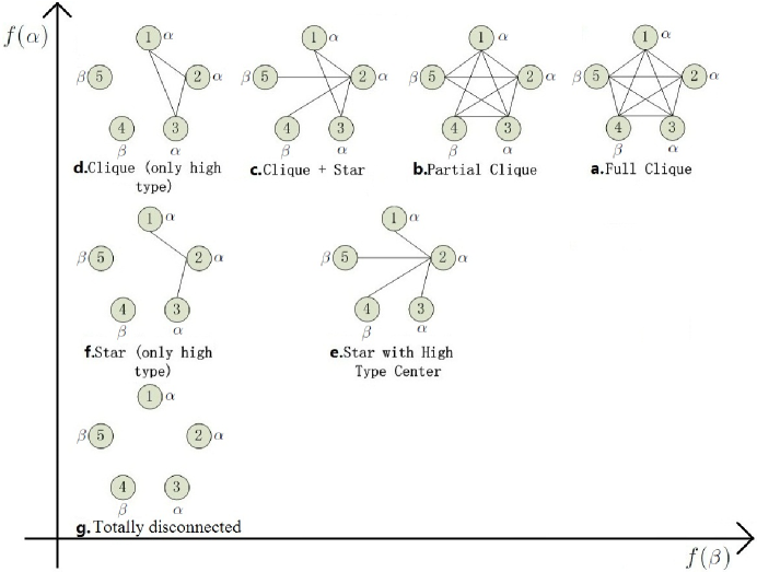
Figure 1: Strongly efficient network in connections model

The following theorem fomally characerizes the conditions on model parameters that lead to each strongly efficient network topology.

Theorem 2.

${\bf{g}}^{e}$ can be described as follows:

• a. If $(1-\delta)f(\beta)>c$, then ${\bf{g}}^{e}$ is a clique encompassing every agent.

• b. If $(1-\delta)\frac{f(\alpha)+f(\beta)}{2}>c>(1-\delta)f(\beta)$, then ${\bf{g}}^{e}$ is such that every two type $\alpha$ agents are linked, and every type $\alpha$ agent is linked with every type $\beta$ agent, but no type $\beta$ agent is linked with another type $\beta$ agent.

• c. If $(1-\delta)f(\alpha)>c>(1-\delta)\frac{f(\alpha)+f(\beta)}{2}$, and $(1+\delta(n_{\alpha}-1))f(\alpha)+(1+\delta(n_{\alpha}+n_{\beta}-2))f(\beta)>2c$, then ${\bf{g}}^{e}$ is such that every two type $\alpha$ agents are linked, and every type $\beta$ agent is linked with the same type $\alpha$ agent, but no type $\beta$ agent is linked with another type $\beta$ agent.

• d. If $(1-\delta)f(\alpha)>c>(1-\delta)\frac{f(\alpha)+f(\beta)}{2}$, and $(1+\delta(n_{\alpha}-1))f(\alpha)+(1+\delta(n_{\alpha}+n_{\beta}-2))f(\beta)<2c$, then ${\bf{g}}^{e}$ is a clique encompassing every type $\alpha$ agent but no type $\beta$ agent.

• e. If $(1-\delta)f(\alpha)<c$, $f(\alpha)+f(\beta)+\delta[(n_{\beta}-1)f(\beta)+(n_{\alpha}-1)(f(\alpha)+f(\beta))]>2c$, and

  $$2(n_{\alpha}-1)f(\alpha)+n_{\beta}(f(\alpha)+f(\beta))+\delta[(n_{\alpha}-1)(n_{\alpha}-2)f(\alpha)+n_{\beta}(n_{\beta}-1)f(\beta)$$

  $$+n_{\beta}(n_{\alpha}-1)(f(\alpha)+f(\beta))]-2(n_{\alpha}+n_{\beta}-1)c>0,$$

  then ${\bf{g}}^{e}$ is a star encompassing every agent, with a type $\alpha$ agent as the center.

• f. If $(1-\delta)f(\alpha)<c$, and

  $$(1+\delta(n_{\alpha}-1))f(\alpha)+(1+\delta(n_{\alpha}+n_{\beta}-2))f(\beta)<2c<f(\alpha)(2+\delta(n_{\alpha}-2)),$$

  then ${\bf{g}}^{e}$ is a star encompassing every type $\alpha$ agent but no type $\beta$ agent.

• g. If $(1-\delta)f(\alpha)<c$, and

  $$\max\{2(n_{\alpha}-1)f(\alpha)+n_{\beta}(f(\alpha)+f(\beta))+\delta[(n_{\alpha}-1)(n_{\alpha}-2)f(\alpha)+n_{\beta}(n_{\beta}-1)f(\beta)$$

  $$+n_{\beta}(n_{\alpha}-1)(f(\alpha)+f(\beta))]-2(n_{\alpha}+n_{\beta}-1)c,f(\alpha)(2+\delta(n_{\alpha}-2))-2c\}<0,$$

  then ${\bf{g}}^{e}$ is the empty network.

Despite the lengthy conditions on the payoffs from different types, the underlying argument for the above characterization is straightforward. According to how much benefit each type can provide via a connection, we can categorize types in a systematic way and assign linkage correspondingly to maximize the sum of total payoffs. For the high types among which a direct link always brings benefits that are higher than the maintenance cost, a clique must be formed among them in any strongly efficient network. The next category contains the types for which any single link to one of the highest types is socially beneficial, but links among themselves are not. As a result, these types will not link directly to themselves but will form every possible link to agents belonging to the first category. When the benefit from a type gets even lower, such types can only add to social welfare by having only one link to one agent of the strictly highest type, thus minimizing the cost and receiving/providing most of the benefit via indirect connection. Last but not least, agents of the lowest types cannot increase the social welfare in any way and will remain singletons in a strongly efficient network.

The connected component of the strongly efficient network exhibits a “core-periphery” pattern in topology. The core, which corresponds to the first category, consists of agents with the highest connectivity degree and the largest clustering coefficient. The periphery agents each have one or more links with the core agents, depending on the value structure. The detailed proof of the theorem is provided below.

• $(a)$ The result is clear since $(1-\delta)f(\beta)>c$ implies that the benefit from any link (bounded below by $2(1-\delta)f(\beta)$) is greater than the associated cost ($2c$).

  $(b)$ If $(1-\delta)\frac{f(\alpha)+f(\beta)}{2}>c$, a link between two type $\alpha$ agents or one type $\alpha$ agent and one type $\beta$ agent always increases the total payoff in the network. Given that there is a link between these agents, $c>(1-\delta)f(\beta)$ implies that a link between two type $\beta$ agents always decreases the total payoff in the network. Hence, ${\bf{g}}^{e}$ is as described in the result.

  $(c)$ The first condition implies that any pair of type $\alpha$ agents are linked in ${\bf{g}}^{e}$. Furthermore, for $n$ type $\beta$ agents with $m_{1},m_{2},\cdots,m_{n}$ links respectively (where $m_{1},m_{2},\cdots,m_{n}$ are positive integers), the largest possible contribution to total payoff is

  $$\sum_{k=1}^{n}[m_{k}(f(\alpha)+f(\beta))+\delta((n_{\alpha}-m_{k})(f(\alpha)+f(\beta))+(n_{\beta}-1)2f(\beta))-2m_{k}c].$$

  Given the condition $c>(1-\delta)\frac{f(\alpha)+f(\beta)}{2}$, the above value is maximized at $m_{k}=1$ for $k=1,2,\cdots,n$. This upper bound is reached when all $n$ type $\beta$ agents are linked to the same type $\alpha$ agent. It is not difficult to see that if the contribution by $n$ type $\beta$ agents is positive, then that by $n+1$ connected type $\beta$ agents is also positive and larger. Hence, in ${\bf{g}}^{e}$, either no type $\beta$ agent is connected, or every type $\beta$ agent is linked to the same type $\alpha$ agent. The condition $(1+\delta(n_{\alpha}-1))f(\alpha)+(1+\delta(n_{\alpha}+n_{\beta}-2))f(\beta)>2c$ implies that the contribution by $n_{\beta}$ type $\beta$ agents is positive, and hence ${\bf{g}}^{e}$ is as described in the result.

  $(d)$ It follows from the proof of $(c)$.

  $(e)$ First, we establish the following lemma.

  Lemma 2.

  Any strongly efficient network has at most one non-empty component.

• Suppose that there exists some strongly efficient network that has two non-empty components $C_{1}$ and $C_{2}$. For component $m$ ($m=1,2$), let $i_{m}$ denote (one of) the agent(s) who has the highest payoff in component $C_{m}$. Since the network is strongly efficient, we know that this payoff is non-negative for $m=1,2$. Let $D_{m}$ be the set of links that $i_{m}$ has in component $C_{m}$. for every $i_{m}j\in D_{m}$ and every $D_{m}^{\prime}\subset D_{m}-i_{m}j$, define

  $$\Delta u_{m}(i_{m}j,D^{\prime}_{m})=u_{{i_{m}}}(\bar{\theta}_{-{i_{m}}},(C_{m}\setminus D_{m})\cup D_{m}^{\prime})-u_{{i_{m}}}(\bar{\theta}_{-{i_{m}}},(C_{m}\setminus D_{m})\cup D_{m}^{\prime}-i_{m}j).$$

  This term denotes the marginal payoff of $i$ from link $i_{m}j$ given $D_{m}^{\prime}$. It is not difficult to see that for $D^{\prime\prime}_{m}\subset D^{\prime}_{m}$, $\Delta u_{m}(i_{m}j,D^{\prime\prime}_{m})\geq\Delta u_{m}(i_{m}j,D^{\prime}_{m})$. Since agent $i_{m}$’s payoff is non-negative, it follows that there must exist $j_{m}$ such that $\Delta u_{m}(i_{m}j,\varnothing)\geq 0$.

  Consider the network $C_{1}\cup C_{2}+j_{1}j_{2}$. For $j_{1}$, the marginal payoff from link $j_{1}j_{2}$ is strictly larger than $\Delta u_{2}(i_{2}j_{2},\varnothing)$; similarly for $j_{2}$, the marginal payoff from link $j_{1}j_{2}$ is strictly larger than $\Delta u_{1}(i_{1}j_{1},\varnothing)$. Hence, the total payoff in this network is strictly higher than that in the original network $C_{1}\cup C_{2}$, which contradicts the assumption that $C_{1}\cup C_{2}$ is strongly efficient. ∎

We then show that if $(1-\delta)f(\alpha)<c$, for every non-empty component ${\bf{g}}$, the total payoff in this component is weakly less than that in a star component with a type $\alpha$ agent as the center, denoted ${\bf{g}}^{*}$. Let $k_{\alpha\alpha}^{d},k_{\alpha\beta}^{d},k_{\beta\beta}^{d}$ denote the number of links between two type $\alpha$ agents, one type $\alpha$ agent and one type $\beta$ agent, and two type $\beta$ agents respectively. Let $k_{\alpha\alpha}^{ind},k_{\alpha\beta}^{ind},k_{\beta\beta}^{ind}$ denote the number of shortest indirect paths between two agents in the same three cases above. Let $\nu({\bf{g}})$ and $\nu({\bf{g}}^{*})$ denote the total payoff in the original component and the star component respectively. Note that the length of any indirect path is at least $2$, and thus we have

$$\nu({\bf{g}})\leq (k_{\alpha\alpha}^{d}+\delta k_{\alpha\alpha}^{ind})2f(\alpha)+(k_{\alpha\beta}^{d}+\delta k_{\alpha\beta}^{ind})(f(\alpha)+f(\beta))+(k_{\beta\beta}^{d}+\delta k_{\beta\beta}^{ind})2f(\beta)$$

$$-2(k_{\alpha\alpha}^{d}+k_{\alpha\beta}^{d}+k_{\beta\beta}^{d})c$$

$$\nu({\bf{g}}^{*})= (n_{\alpha}-1+\delta\frac{(n_{\alpha}-1)(n_{\alpha}-2)}{2})2f(\alpha)+(n_{\beta}+\delta n_{\beta}(n_{\alpha}-1))(f(\alpha)+f(\beta))$$

$$+\delta\frac{n_{\beta}(n_{\beta}-1)}{2}2f(\beta)-2(n_{\alpha}+n_{\beta}-1)c.$$

Note that

$$k_{\alpha\alpha}^{d}+k_{\alpha\alpha}^{ind} =\frac{n_{\alpha}(n_{\alpha}-1)}{2}$$

$$k_{\alpha\beta}^{d}+k_{\alpha\beta}^{ind} =n_{\alpha}n_{\beta}$$

$$k_{\beta\beta}^{d}+k_{\beta\beta}^{ind} =\frac{n_{\beta}(n_{\beta}-1)}{2}.$$

Then we have

$$\nu({\bf{g}})-\nu({\bf{g}}^{*})\leq (1-\delta)((k_{\alpha\alpha}^{d}-(n_{\alpha}-1))2f(\alpha)+(k_{\alpha\beta}^{d}-n_{\beta})(f(\alpha)+f(\beta))+k_{\beta\beta}^{d}2f(\beta))$$

$$-2(k_{\alpha\alpha}^{d}+k_{\alpha\beta}^{d}+k_{\beta\beta}^{d}-(n_{\alpha}+n_{\beta}-1))c$$

$$\leq 2(k_{\alpha\alpha}^{d}+k_{\alpha\beta}^{d}+k_{\beta\beta}^{d}-(n_{\alpha}+n_{\beta}-1))((1-\delta)f(\alpha)-c)$$

$$\leq 0.$$

Finally, note that equality is achieved if and only if (1) $k_{\alpha\beta}^{d}=k_{\beta}$, $k_{\beta\beta}^{d}=0$, $k_{\alpha\alpha}^{d}+k_{\alpha\beta}^{d}+k_{\beta\beta}^{d}=n_{\alpha}+n_{\beta}-1$ and (2) there is no (shortest) indirect path with length greater than two between any two type $\alpha$ agents. These two conditions are satisfied if and only if ${\bf{g}}$ is also a star component with a type $\alpha$ agent as the center.

It is clear that if a star component with a type $\alpha$ agent as the center results in a positive total payoff, then adding an agent of type $\alpha$ as the periphery will increase the total payoff; moreover, if the marginal payoff brought about by all the type $\beta$ agents in the star component is positive, then adding an agent of type $\beta$ as the periphery will increase the total payoff. Hence, ${\bf{g}}^{e}$ can only be one of the following three: (1) the empty network, (2) a star encompassing only type $\alpha$ agents, and (3) a star encompassing all agents, with a type $\alpha$ agent as the center. The second and the third conditions in the result ensure that the marginal payoff brought about by all the type $\beta$ agents is positive, and that (3) has a positive total payoff. Hence, (3) is ${\bf{g}}^{e}$.

$(f)$ It follows from the proof of $(e)$.

$(g)$ It follows from the proof of $(e)$. ∎

5.2 Strong Efficiency and Core-Stability

The connections model also allows us to investigate the relation between a strongly efficient network and a core-stable network. Note that these two concepts do not imply one another. In a strongly efficient network, there may be a subgroup of agents that can improve the payoff of each member by “local autonomy”: for instance, the center of a star will be strictly better off staying a singleton if all periphery agents are of low type. On the other hand, even though the agents cannot improve everyone’s payoff in a core-stable network, there may be a way to improve the total payoff. An example would be to switch the center of a star from a low type agent to a high type one.

In this section, we establish necessary and sufficient conditions for a strongly efficient network to be core-stable. It is helpful to first compute the largest possible one-period payoff an agent of each type can get in any network.

Proposition 5.

For $\theta\in{\alpha,\beta}$ let $V(\theta)$ denote the maximum payoff that an agent of type $\theta$ can obtain in any network in a single period. We have:

• a. If $(1-\delta)f(\beta)>c$, then

  $$V(\alpha) =(n_{\alpha}-1)f(\alpha)+n_{\beta}f(\beta)-(n_{\alpha}+n_{\beta}-1)c$$

  $$V(\beta) =n_{\alpha}f(\alpha)+(n_{\beta}-1)f(\beta)-(n_{\alpha}+n_{\beta}-1)c.$$

• b. If $(1-\delta)f(\alpha)>c>(1-\delta)f(\beta)$, then

  $$V(\alpha) =(n_{\alpha}-1)f(\alpha)+\delta n_{\beta}f(\beta)-(n_{\alpha}-1)c$$

  $$V(\beta) =n_{\alpha}f(\alpha)+\delta(n_{\beta}-1)f(\beta)-n_{\alpha}c.$$

• c. If $\min\{f(\alpha)+\delta((n_{\alpha}-2)f(\alpha)+n_{\beta}f(\beta)),f(\alpha)+\delta((n_{\alpha}-1)f(\alpha)+(n_{\beta}-1)f(\beta))\}>c>(1-\delta)f(\alpha)$, then

  $$V(\alpha) =f(\alpha)+\delta((n_{\alpha}-2)f(\alpha)+n_{\beta}f(\beta))-c$$

  $$V(\beta) =f(\alpha)+\delta((n_{\alpha}-1)f(\alpha)+(n_{\beta}-1)f(\beta))-c.$$

• d. If $f(\alpha)+\delta((n_{\alpha}-1)f(\alpha)+(n_{\beta}-1)f(\beta))>c>\max\{f(\alpha)+\delta((n_{\alpha}-2)f(\alpha)+n_{\beta}f(\beta)),(1-\delta)f(\alpha)\}$, then

  $$V(\alpha) =0$$

  $$V(\beta) =f(\alpha)+\delta((n_{\alpha}-1)f(\alpha)+(n_{\beta}-1)f(\beta))-c.$$

• e. If $\max\{f(\alpha)+\delta((n_{\alpha}-1)f(\alpha)+(n_{\beta}-1)f(\beta)),f(\alpha)+\delta((n_{\alpha}-2)f(\alpha)+n_{\beta}f(\beta)),(1-\delta)f(\alpha)\}<c$, then

  $$V(\alpha) =0$$

  $$V(\beta) =0.$$

• $(a)$ Let $\hat{V}(\theta,m)$ be the largest possible payoff of an agent of type $\theta$ with $m$ links. We have

  $\hat{V}(\alpha,m)=\left\{\begin{array}[]{c}0,\text{ if $m=0$}\\ mf(\alpha)+\delta((n_{\alpha}-1-m)f(\alpha)+n_{\beta}f(\beta))-mc,\text{ if $0<m\leq n_{\alpha}-1$}\\ (n_{\alpha}-1)f(\alpha)+(m-(n_{\alpha}-1))f(\beta)+\delta(n_{\alpha}+n_{\beta}-1-m)f(\beta)-mc,\text{ otherwise}\end{array}\right.$ $\hat{V}(\beta,m)=\left\{\begin{array}[]{c}0,\text{ if $m=0$}\\ mf(\alpha)+\delta((n_{\alpha}-m)f(\alpha)+n_{\beta}f(\beta))-mc,\text{ if $m\leq n_{\alpha}$}\\ n_{\alpha}f(\alpha)+(m-n_{\alpha})f(\beta)+\delta(n_{\alpha}+n_{\beta}-1-m)f(\beta)-mc,\text{ otherwise.}\end{array}\right.$

It is clear that these largest possible payoffs are achievable (for instance, let the agent be a periphery agent in a star with a type $\alpha$ agent as the center, and form the rest of the $m$ links first with type $\alpha$ agents, then with type $\beta$ agents if she is already linked with every type $\alpha$ agent.). If $(1-\delta)f(\beta)>c$, for an agent of either type her payoff is maximized when she makes every possible link, hence $V(\alpha)$ and $V(\beta)$ are as shown in the result.

$(b)$ If $(1-\delta)f(\alpha)>c>(1-\delta)f(\beta)$, for an agent of either type her payoff is maximized when she links with every type $\alpha$ agent but with no type $\beta$ agent, hence $V(\alpha)$ and $V(\beta)$ are as shown in the result.

$(c)$ If $c>(1-\delta)f(\alpha)$, given that an agent is connected (not a singleton), her largest payoff is higher when she has fewer links. Hence, her payoff is $\hat{V}(\theta,1)$ if $\hat{V}(\theta,1)\geq 0$ and $0$ otherwise. Hence $V(\alpha)$ and $V(\beta)$ are as shown in the result.

$(d)$ It follows from the proof of $(c)$.

$(e)$ It follows from the proof of $(c)$. ∎

We can see from the proof above that the largest payoff an agent obtains from a network is closely related to the network topology. Hence, if a network offers the largest possible payoff to most of the agents, it is very likely to be core-stable since those agents’ payoffs cannot be improved further. The final criterion of stability then rests on whether the few agents that do not get the highest possible payoff can form a beneficial coalition. Using this argument, we inspect the strongly efficient network in every possible type vector and present the result below.

Proposition 6.

Consider cases ($a$) – ($g$) in Theorem 2. We have:

• a, d, g. ${\bf{g}}^{e}$ is core-stable.

• b. ${\bf{g}}^{e}$ is core-stable if and only if $f(\beta)\geq c$.

• c. ${\bf{g}}^{e}$ is core-stable if and only if a network that links one type $\alpha$ agent to all the type $\beta$ agents yields the $\alpha$ agent a non-negative payoff.

• e. ${\bf{g}}^{e}$ is core-stable if and only if a network that has a type $\alpha$ agent at the center yields the $\alpha$ agent a non-negative payoff.

• f. ${\bf{g}}^{e}$ is core-stable if and only if $f(\alpha)\geq c$.

• $(a)(d)(g)$ The cases $(a)$ and $(g)$ are clear. For $(d)$, suppose that ${\bf{g}}^{e}$ is not core-stable, it then follows that any blocking group $I^{\prime}$ (with network ${\bf{g}}^{\prime}$) must contain at least one type $\alpha$ agent, but not all type $\alpha$ agents. Consider the network ${\bf{g}}^{\prime}$ that blocks ${\bf{g}}^{e}$. Since every agent in $I^{\prime}$ has a weakly higher payoff in ${\bf{g}}^{\prime}$ than in ${\bf{g}}^{e}$ and some agent in $I^{\prime}$ has a strictly higher payoff in ${\bf{g}}^{\prime}$ than in ${\bf{g}}^{e}$, the total payoff of agents in $I^{\prime}$ must be strictly higher than that in ${\bf{g}}^{e}$. By Theorem 2, we can re-organize ${\bf{g}}^{\prime}$ into a clique with only type $\alpha$ agents to yield an even higher total payoff. However, if a clique with only type $\alpha$ agents has a positive total payoff, then it is impossible for a proper subset of these agents to form a clique with a higher total payoff than their total payoff in the original clique. Hence we have a contradiction.

  $(b)$ If $f(\beta)<c$, then ${\bf{g}}^{e}$ is not core-stable because a clique formed by all type $\alpha$ agents blocks ${\bf{g}}^{e}$. Suppose that $f(\beta)\geq c$ and that ${\bf{g}}^{e}$ is not core-stable, then any blocking group $I^{\prime}$ either only contains type $\alpha$ agents, or contains all the agents because each type $\beta$ agent in ${\bf{g}}^{e}$ gets payoff $V(\beta)$, and getting $V(\beta)$ requires connection to every other agent. Both cases contradict the fact that ${\bf{g}}^{e}$ is strongly efficient.

  $(c)$ Let $i$ denote the type $\alpha$ agent linking with all the type $\beta$ agents. If $i$ has a negative payoff, then ${\bf{g}}^{e}$ is not core-stable because $\{i\}$ blocks ${\bf{g}}^{e}$. Suppose that $i$ has a non-negative payoff and that ${\bf{g}}^{e}$ is not core-stable, then any blocking group $I^{\prime}$ either only contains no type $\alpha$ agent other than $i$ and at least one type $\beta$ agent, or contains all the agents because each type $\alpha$ agent other than $i$ in ${\bf{g}}^{e}$ gets payoff $V(\alpha)$, and getting $V(\alpha)$ requires connection to every other agent. The second case contradicts the fact that ${\bf{g}}^{e}$ is strongly efficient. In the first case, note that the largest payoff of any type $\beta$ agent in $I^{\prime}$ is strictly less than $\hat{V}(\beta,1)$ (since $c>(1-\delta)f(\beta)$), which is the payoff of every type $\beta$ agent in ${\bf{g}}^{e}$. Hence we again have a contradiction.

  $(e)$ Let $j$ denote the type $\alpha$ agent at the center. If $j$ has a negative payoff, then ${\bf{g}}^{e}$ is not core-stable because $\{j\}$ blocks ${\bf{g}}^{e}$. Suppose that $j$ has a non-negative payoff and that ${\bf{g}}^{e}$ is not core-stable, then any blocking group $I^{\prime}$ either only contains $j$, or contains all the agents because each agent other than $j$ in ${\bf{g}}^{e}$ gets payoff $V(\alpha)$ (or $V(\beta)$), and getting $V(\alpha)$ (or $V(\beta)$) requires connection to every other agent. The first case contradicts the assumptions that $I^{\prime}$ blocks ${\bf{g}}^{e}$ and $j$ has a non-negative payoff in ${\bf{g}}^{e}$, and the second case contradicts the fact that ${\bf{g}}^{e}$ is strongly efficient.

  $(f)$ If $f(\alpha)<c$, then ${\bf{g}}^{e}$ is not core-stable because the center agent in ${\bf{g}}^{e}$ blocks ${\bf{g}}^{e}$. Suppose that $f(\alpha)\geq c$ and that ${\bf{g}}^{e}$ is not core-stable, it then follows that any blocking group $I^{\prime}$ (with network ${\bf{g}}^{\prime}$) must contain at least one type $\alpha$ agent, but not all type $\alpha$ agents. Consider the network ${\bf{g}}^{\prime}$ that blocks ${\bf{g}}^{e}$. Since every agent in $I^{\prime}$ has a weakly higher payoff in ${\bf{g}}^{\prime}$ than in ${\bf{g}}^{e}$ and some agent in $I^{\prime}$ has a strictly higher payoff in ${\bf{g}}^{\prime}$ than in ${\bf{g}}^{e}$, the total payoff of agents in $I^{\prime}$ must be strictly higher than that in ${\bf{g}}^{e}$. By Proposition 2, we can re-organize ${\bf{g}}^{\prime}$ into a star with only type $\alpha$ agents to yield an even higher total payoff. However, if $f(\alpha)\geq c$, it is impossible for a proper subset of the type $\alpha$ agents to form a star with a higher total payoff than their total payoff in ${\bf{g}}^{e}$. Hence we have a contradiction. ∎

The key to whether a strongly efficient network is core-stable is its “weakest link”: the agent maintaining the most links but enjoying the smallest net payoff. If this particular agent gets a negative payoff, she would prefer to simply sever all her links and remain a singleton.

5.3 Effect of Spatial Discount

A crucial factor in the connections model is the spatial discount factor $\delta$. It determines the rate of payoff depreciation as two agents become further apart in connection, and hence influences an agent’s incentives of directly linking to another already connected agent. As a result, a change in $\delta$ affects every connected agent’s payoff and has a non-negligible impact on the set of sustainable networks in equilibrium. The importance of the spatial discount in a static environment and a dynamic one with myopia has been noted in Jackson and Wolinsky[18] and Song and van der Schaar[31]. In the dynamics with foresight, the role of $\delta$ becomes even more important than the previous cases because it enters the payoff an agent obtains for every period. As it turns out, the set of sustainable networks changes monotonically with the value of $\delta$.

Given $\bar{\theta}$, let $G(\delta)$ denote the set of networks ${\bf{g}}$ for which there is a cutoff $\bar{\gamma}\in(0,1)$ such that if $\gamma\in[\bar{\gamma},1)$, then there exists an equilibrium in which the formation process converges strongly to ${\bf{g}}$.

Proposition 7.

If $\delta_{1}>\delta_{2}$, then $G(\delta_{1})\supset G(\delta_{2})$.

• For every ${\bf{g}}\in G(\delta_{2})$, it follows from Theorem $1(a)$ that every connected agent in ${\bf{g}}$ gets a non-negative payoff when $\delta=\delta_{2}$. Since $\delta_{1}>\delta_{2}$, every connected agent in ${\bf{g}}$ gets a positive payoff when $\delta=\delta_{1}$. Then by Theorem $1$ we know that ${\bf{g}}\in G(\delta_{1})$. ∎

Although the set of networks that are sustainable in equilibrium is monotone in $\delta$, the strongly efficient networks that are sustainable in equilibrium is not monotone in $\delta$. Consider the following example: $f(\alpha)=3$, $f(\beta)=0.5$, $c=2$, $n_{\alpha}=1$ and $n_{\beta}=3$. From the previous analysis, we know that the strongly efficient network is either a star with the type $\alpha$ agent as the center, or empty. On one hand, when $\delta$ is low (for instance $\delta=0.1$) the efficient network is empty and clearly can be supported in equilibrium. On the other hand, when $\delta$ is high (for instance $\delta=0.8$) the efficient network is a star. However, it is clear that a star network cannot be supported in equilibrium since the center agent has a negative payoff. Even though a higher $\delta$ sustains a larger set of networks, the strongly efficient network changes with $\delta$ as well.

The spatial discount also partially determines the required patience level of agents to sustain a network in equilibrium. When $\delta$ changes in a way that forming/maintaining links becomes more beneficial to oneself in every period, every connected agent in a network has higher incentive, and at the same time needs less patience, to sustain that network in the long run. We demonstrate this by using our constructed equilibrium $\hat{s}_{c}$. Given $\bar{\theta}$, $K$ and ${\bf{g}}$, let $\gamma(\delta)$ denote the smallest $\gamma$ such that $\hat{s}_{c}$ is an equilibrium (if such $\gamma$ exists) under spatial discount $\delta$.

Proposition 8.

There exists $\hat{\delta}\leq 1$ such that for every $\delta_{1}$, $\delta_{2}\in[0,\hat{\delta}]$ such that $\delta_{1}>\delta_{2}$ and both $\gamma(\delta_{1})$ and $\gamma(\delta_{2})$ exist, $\gamma(\delta_{1})<\gamma(\delta_{2})$.

• Note that the only incentive problem faced by an agent is whether to sever or refuse to form a link in ${\bf{g}}$ during the cooperation phase. Doing so saves the agent the cost $c$, and the agent’s loss in benefit has the form of

  $$\sum_{l=1}^{L}(\delta^{a_{l}}-\delta^{b_{l}})f(\theta_{j_{l}})$$

  where $a_{l}\in\mathbb{N}$, $b_{l}\in\mathbb{N}\cup\{\infty\}$ satisfy $a_{l}<b_{l}$. When $b_{l}=\infty$, clearly $\delta^{a_{l}}-\delta^{b_{l}}$ is increasing in $\delta$. When $b_{l}\in\mathbb{N}$, we have

  $$\frac{d(\delta^{a_{l}}-\delta^{b_{l}})}{d\delta}=a_{l}\delta^{a_{l}-1}-b_{l}\delta^{b_{l}-1}=\delta^{a_{l}-1}(a_{l}-b_{l}\delta^{b_{l}-a_{l}})$$

  This derivative is positive when $\delta$ is sufficiently small. In other words, the benefit from an existing link is increasing in $\delta$ when $\delta$ is sufficiently small. Let $\hat{\delta}\leq 1$ be the largest $\delta$ such that every $\delta\in[0,\hat{\delta}]$ satisfies this property.

  Consider $\delta_{1}$, $\delta_{2}\in[0,\hat{\delta}]$ such that $\delta_{1}>\delta_{2}$ and both $\gamma(\delta_{1})$ and $\gamma(\delta_{2})$ exist, and $\gamma\geq\gamma(\delta_{2})$. Note that by the above property, in any period during the cooperation phase, the benefit from following the equilibrium strategy in the current period and in every subsequent period is increasing in $\delta$, and the cost stays the same. Hence, if $\hat{s}_{c}^{y_{c}}$ is an equilibrium given $\delta_{2}$ and $\gamma$, it must also be an equilibrium given $\delta_{1}$ and $\gamma$. We can then conclude that $\gamma(\delta_{1})<\gamma(\delta_{2})$. ∎

5.4 Generalized Connections Model

In this section, we generalize the above two-type connections model to a much richer multi-type environment. Consider a type set $\Theta$ with finitely many types, and let the payoff of agent $i$ from connecting to agent $j$ be $f(\theta_{j})$ before spatial discount. Our results on the unique efficient network and stability can be easily extended to this model. The unique efficient network ${\bf{g}}^{e}$ has a general core-periphery structure, characterized by a partition of agents $\{I_{1},I_{2},I_{3},I_{4}\}$ induced by a triplet of types $\{\theta^{1},\theta^{2},\theta^{3}\}$ such that $f(\theta^{1})\geq f(\theta^{2})\geq f(\theta^{3})$ :

• a. Core $I_{1}=\{i:f(\theta_{i})\geq f(\theta^{1})\}$: the maximal subset of inter-linked agents.

• b. Periphery I $I_{2}=\{i:f(\theta^{2})\leq f(\theta_{i})<f(\theta^{1})\}$: the maximal subset of agents that do not belong to $I_{1}$ but link to every agent of some type(s) in $I_{1}$.

• c. Periphery II $I_{3}=\{i:f(\theta^{3})\leq f(\theta_{i})<f(\theta^{2})\}$: the maximal subset of agents that do not belong to $I_{1}\cup I_{2}$ but link to the same agent in $I_{1}$.

• d. Singleton $I_{4}=\{i:f(\theta_{i})<f(\theta^{3})\}$: the maximal subset of agents that do not link to any other agent.

In the unique efficient network all agents in the core are linked to each other, all agents in periphery I are linked to all agents of at least one type in the core, all agents in periphery II are linked and only linked to the same agent in the core, and agents that are singletons are unlinked. Figure 2 below illustrates a sample core-periphery network, with one type in each category.

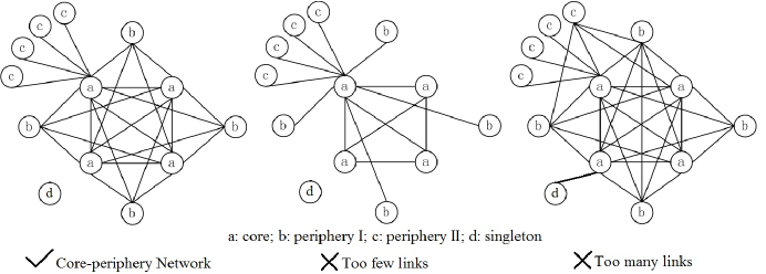
Figure 2: Sample core-periphery network

The type cutoffs, $\{\theta^{1},\theta^{2},\theta^{3}\}$, are determined in a similar way to the two-type model, only with more tedious calculations on an agent’s maximum possible contribution to the total payoff of the group. A rough intuition for this result is that an agent of a higher type takes more responsibility, in the sense that she should form more links to create more value for the greater good. The overall distinguishing features of the efficient network, especially when the number of agents gets large, include a small diameter, a large ratio between number of links and number of agents, and a large ratio of number of “triangles” (connected triples of agents) and number of agents. We show in the next section that in realistic situations where the connections model applies, the level of coordination among individuals is significantly higher than predicted by previous theories, and that our model with foresight can account for a considerable proportion of cooperation behavior in these endogenously formed networks.

Next, we can derive a necessary and sufficient condition for the efficient network to be core-stable: an efficient network is core-stable if and only if the agent(s) of the highest type has a non-negative payoff. The argument underlying the “if” part of this result (the “only if” part is clear) is similar to the proof of Proposition 5. Suppose that there is a blocking group $I^{\prime}$ and a corresponding network ${\bf{g}}^{\prime}$ on $I^{\prime}$ that yields a weakly higher payoff for every agent in $I^{\prime}$ and a strictly higher payoff for at least one agent in $I^{\prime}$. We can always re-organize ${\bf{g}}^{\prime}$ according to Theorem 2 to obtain a weakly higher total payoff for the group $I^{\prime}$; then the agent with the highest payoff in the new network must be at least as better-off as she is in ${\bf{g}}^{e}$. This agent cannot belong to $I_{2}$ or $I_{3}$ since the agents in these two categories in ${\bf{g}}^{e}$ have already enjoyed the unique highest possible payoff that can only be provided by ${\bf{g}}^{e}$; however, if this agent belongs to $I_{1}$, then it must be the case that some other agent in $I_{2}$ gets a lower payoff than in ${\bf{g}}^{e}$, a contradiction. An important message conveyed by this result is that for efficiency to be achieved in equilibrium and to prevent coalitional deviation, it is sufficient to focus on the agents of the highest type, ensuring that their cost of maintaining links are covered by the benefit from connection.

5.5 Empirical Comparisons

We have provided a full characterization of the strongly efficient network in a standard connections model with heterogeneous agents, in which we find that such networks generally exhibit a “core-periphery” structure. Prominent features of such network topologies in terms of several descriptive statistics are: (1) a large average local clustering coefficient (ALCC), measured by the number of pairs of linked neighbors devided by the number of possible pairs of neighbors; (2) a large global clustering coefficient, measured by the number of closed triangles devided by the number of triangles; (3) a short diameter (D), measured by the number of links in the longest of all shortest paths between any two agents). Both clustering coefficients indicate the degree to which small groups of agents in a network tend to keep close ties to each other, and the diameter is an index of the entire network’s density. Note that a large clustering coefficient does not guarantee a small diameter. For instance, a “chain” network created by connecting many small cliques has a large clustering coefficient but a large diameter.

Our findings are consistent with data collected from existing real networks. To see this, we compare our predictions with data obtained from sample social networks from Facebook and collaboration networks of Arxiv High Energy Physics (AHEP) , and also with simulated networks following models with myopic agents, using pairwise stability introduced by Jackson and Wolinsky[18] as the solution concept in each period. In the simulation “Myopic 1”, we assume that the payoff from connecting to any one agent before spatial discount is 10, the link maintenance cost is 5, and the spatial discount factor is 0.6. In the simulation “Myopic 2”, we assume that there are three types of agents; connecting to each type yields a payoff of 16, 10 and 6 before spatial discount respectively, and the cost and the spatial discount factor remain the same. The ratio of types is $1:2:3$, that is type 1, 2 and 3 agents account for $\frac{1}{6}$, $\frac{1}{3}$ and $\frac{1}{2}$ of the population correspondingly. The simulated network formation process is run for a sufficiently long time such that each pair of agents is selected at least twice in expectation. The “Foresighted Model” column shows descriptive statistics for the strongly efficient network in our model, with the same group size and type distribution as “Myopic 2”. Table 1 below provides summary statistics on the networks and Figure 3 illustrates the actual network topology in AHEP. In Table 1, the entry “90% D” represents the 90th percentile in the distribution of path length.

We find that the actual networks recorded are considerably closer to those predicted by our model with foresighted agents than by models with myopic agents which are representative of much previous literature. In the two models with myopia, the network is not clustered (small ALCC and GCC), suggesting a relatively small group of “super star” agents that link to many “periphery” agents, but showing little direct relation among the “periphery” agents. This is not true for the actual networks (large ALCC and GCC). In contrast, the strongly efficient network we have characterized captures this charateristics of high clustering, and we have shown that when agents are foresighted this network can be supported in equilibrium. It corroborates our earlier statement that our model with foresight provides a more appropriate framework of analyzing network formation, which leads to more realistic predictions for actual networks.

Another observation that can be made based on these results is that the formed networks are rather dense (small D), confirming the well-studied “small world” phenomenon. However, the diameter of an actual network is typically larger than that predicted by the network formations models. We believe that this difference in diameter results from the simplistic meeting process adopted in all this literature: individuals in an actual network do not meet with uniform probabilities; instead, some agents may meet more often while others only seldom. Hence, we believe that an important topic of future research is understanding the effect of different meeting processes on the emerging networks.

	Actual		Simulation		Foresighted Model
	Facebook	AHEP	Myopic 1	Myopic 2
$N$	4039	12008	1000	1000	1000
ALCC	0.6055	0.6115	0.1357	0.1957	0.4251
GCC	0.2647	0.3923	0.0458	0.0756	0.3570
D	8	13	2	2	2
90% D	4.7	5.3	2	2	2

Table 1: Summary statistics of networks

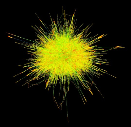
Figure 3: AHEP network

6 Network Convergence Theorem with Incomplete Information

In real-life applications, agents will not usually know the types of the other agents before they are linked to them. As we have shown in our prior work in[31], the introduction of incomplete information leads to significant differences in agents’ strategic behavior and equilibrium network topology. In this section, we extend the Network Convergence Theorem to the environment with incomplete information. Surprisingly, we are able to identify an undemanding condition on the payoff structure under which the formation process will again converge even in this setting to the strongly efficient network in equilibrium.

6.1 Modeling Incomplete Information

At the beginning of $t=1$, each agent only knows her own type and holds the prior belief (that types are i.i.d. according to $H$) on other agents’ types.

Let $\mathcal{B}=\Delta(\Theta^{N})$ denote the set of possible beliefs on the type vector. A (pure) strategy of agent $i$ is now a mapping

$$s_{i}:\mathcal{B}\times I-i\times Y\times\Omega\times Z\rightarrow\mathcal{A},$$

with the same constraint $s_{i}(\cdot,\cdot,\cdot,0,0)\equiv 0$. An equilibrium is similarly defined as before, except for the additional requirement that $i$ maximizes her expected discounted total payoff given her belief at every period.

Let $B_{i}:Y\rightarrow\mathcal{B}$ denote agent $i$’s belief updating function, which is a mapping from the set of possible public signals to the set of possible beliefs. We assume that it satisfies the following properties:

• 1. $i$ knows her own type: regardless of $\sigma(t)$, she puts probability $1$ on her true type.

• 2. $i$ knows the type of any agent that she has been connected to: if some ${\bf{g}}$ such that $ij\in{\bf{g}}$ has ever been formed in $\sigma(t)$, then $i$ always puts probability $1$ on $j$’s true type starting from period $t$.

• 3. Agents use Bayesian updating whenever possible. We adopt the convention that when Bayes rule does not apply, agents maintain the same priors.

We now define some concepts related to the payoff structure that will be useful in constructing equilibrium strategies later. First we define a partial equilibrium network for a subset of agents.

Definition 6 (Partial equilibrium network).

Given $\bar{\theta}$, a network ${\bf{g}}$ formed in $I^{\prime}\subset I$ is a partial equilibrium network for $I^{\prime\prime}\subset I^{\prime}$ if (1) each agent in $I^{\prime\prime}$ gets a positive payoff from ${\bf{g}}$; (2) no agent in $I^{\prime\prime}$ can increase her payoff by severing any of her links in ${\bf{g}}$.

Given a subset of agents $I^{\prime}$ and the associated type vector $\bar{\theta}_{I^{\prime}}$, consider a function $r:\Theta^{|I^{\prime}|}\rightarrow G_{I^{\prime}}$. We define the following property for $r$:

Definition 7 (Admissible function).

We say that $r$ is an admissible function for $I^{\prime}$ if for every $\bar{\theta}_{I^{\prime}}\in\Theta^{|I^{\prime}|}$, $r(\bar{\theta}_{I^{\prime}})$ is a network such that (1) every non-singleton agent in $r(\bar{\theta}_{I^{\prime}})$ has a positive payoff; (2) there exists a partial equilibrium network in $G_{I^{\prime}}$ for the set of singleton agents in $r(\bar{\theta}_{I^{\prime}})$, denoted as $r^{\prime}(\bar{\theta}_{I^{\prime}})$. We say that $I^{\prime}$ is admissible if there exists an admissible function $r$ for $I^{\prime}$.

In a partial equilibrium network, no agent has incentive to unilaterally sever any of her links; hence, the name “partial equilibrium”. Then (the existence of) an admissible function essentially characterizes a particular type of agent subgroup: it maps every type vector in the subgroup to a network that provides every connected agent a positive payoff, and at the same time guarantees the existence of a partial equilibrium network for the set of singleton agents. Intuitively, the former network can be sustained in the long run when agents are patient, and the latter can be used as a way to reward the future singleton agents for their revelation of private information. We will construct an equilibrium strategy profile following this argument in the next section.

In many cases, the whole agent set $I$ is admissible. One of the simplest scenarios is that for every type vector there exists a network yielding a positive payoff for every agent, so that a partial equilibrium network will not even be necessary because the set of singleton agents will be empty. For instance, consider the connections model discussed before, and consider the following two-type scenario: $\Theta=\{\alpha,\beta\}$, $N=5$, $f(\alpha)>c>f(\beta)$, $(1+\delta)f(\beta)>c$, and $f(\alpha)+3f(\beta)>3c$. First, note that when there exists at least one type $\alpha$ agent, a partial equilibrium network for any number of type $\beta$ agents is a star network with a type $\alpha$ agent as the center. Then the following function $r$ is an admissible function for $I$:

$r(\bar{\theta})=\left\{\begin{array}[]{c}\text{Star network with type $\alpha$ center, if at least two agents are of type $\alpha$}\\ \text{Wheel network, otherwise.}\end{array}\right.$

It is easy to verify that $r$ is indeed admissible for $I$. Moreover, it is also straight forward to show that $r$ maps $\bar{\theta}$ to the strongly efficient network whenever the strongly efficient network gives every agent a positive payoff. In this type of payoff structure, the larger $N$ is, the more likely such a simple admissible function for $I$ exists. When $N$ is large, even if $f(\alpha)$ and $f(\beta)$ are both small relative to $c$, a topology such as a star or a wheel may still ensure a positive payoff for every agent. In the case where $r$ maps a type vector to some unconnected network (a network with singleton agents), a star or a wheel can be used as partial equilibrium networks (in the case of a star, the singleton agents in $r$ would be placed in the periphery).

6.2 Construction of Equilibrium Strategies

As with complete information, we explicitly construct a strategy profile that will constitute an equilibrium when agents are sufficiently patient. First we specify the associated monitoring structure, denoted $y_{ic}$. Similarly to the case with complete information, $y_{ic}$ measures the least informative monitoring structure needed for our network convergence theorem.

To simplify the description of $y_{ic}$, we first introduce some additional notations. For a given time period $t$ and a given subgroup of agents $I^{\prime}\subset I$, we denote as $I^{\prime\prime}_{1}({\bf{g}},t)$ the subset of agents in $I^{\prime}$ that failed to form/maintain a link in ${\bf{g}}$ when possible, and as $I^{\prime\prime}_{2}(t)$ the subset of agents in $I^{\prime}$ that formed/maintained a link between $I^{\prime}$ and $I\setminus I^{\prime}$. We let $\hat{{\bf{g}}}_{I^{\prime}}$ denote the clique on $I^{\prime}$. Finally, we say that information is complete within $I^{\prime}$ if every agent knows the type of every other agent in $I^{\prime}$, and that information is incomplete within $I^{\prime}$ otherwise. Denote these events in period $t$ as $O_{c}(I^{\prime},t)$ and $O_{ic}(I^{\prime},t)$.

• 1. $Y=\{X_{0},X_{1},T,E_{C},E_{P}\}\times 2^{I}$. The subset of $I$ in the second argument represents the subgroup of non-solitary agents, and $X_{0},X_{1},T,E_{C},E_{P}$ represent five phases with respect to this subgroup: the experimentation phase with incomplete information, experimentation phase with complete information, transition phase, exploitation phase with cooperation and exploitation phase with punishment correspondingly. We will define and explain these concepts later.

• 2. $y_{ic}(\sigma(0))=(X_{0},I)$.

• 3. In period $t\geq 1$, for every pair of agents $i,j\in I^{\prime}\subset I$:

  • a. If $y_{ic}(\sigma(t-1))=(X_{0},I^{\prime})$:

    $$O_{c}(I^{\prime}\setminus I^{\prime\prime}_{1}(\hat{{\bf{g}}}_{I^{\prime}},t),t) \rightarrow y_{ic}(\sigma(t))=(T,I^{\prime}\setminus I^{\prime\prime}_{1}(\hat{{\bf{g}}}_{I^{\prime}}),t)$$

    $$O_{ic}(I^{\prime}\setminus I^{\prime\prime}_{1}(\hat{{\bf{g}}}_{I^{\prime}},t),t) \rightarrow y_{ic}(\sigma(t))=(X_{0},I^{\prime}\setminus I^{\prime\prime}_{1}(\hat{{\bf{g}}}_{I^{\prime}}),t).$$

  • b. If $y_{ic}(\sigma(t-1))=(X_{1},I^{\prime})$: $y_{ic}(\sigma(t))=(T,I^{\prime}\setminus(I^{\prime\prime}_{1}(r^{\prime}(\bar{\theta}_{I^{\prime}}),t)\cup I^{\prime\prime}_{2}(t)))$.

  • c. If $y_{ic}(\sigma(t-1))=(T,I^{\prime})$: $y_{ic}(\sigma(t))=(E_{C},I^{\prime})$ if $r^{\prime}(\bar{\theta}_{I^{\prime}})$ has been the network topology within $I^{\prime}$ (including no link between $I^{\prime}$ and $I\setminus I^{\prime}$) for a fixed number of $J$ consecutive periods. Otherwise, $y_{ic}(\sigma(t))=(T,I^{\prime}\setminus(I^{\prime\prime}_{1}(r^{\prime}(\bar{\theta}_{I^{\prime}}),t)\cup I^{\prime\prime}_{2}(t)))$.

  • d. If $y_{ic}(\sigma(t-1))=(E_{C},I^{\prime})$:

    $$I^{\prime\prime}_{1}(r(\bar{\theta}_{I^{\prime}}),t)\cup I^{\prime\prime}_{2}(t)=\varnothing \rightarrow y_{ic}(\sigma(t))=(E_{C},I^{\prime})$$

    $$I^{\prime\prime}_{1}(r(\bar{\theta}_{I^{\prime}}),t)\cup I^{\prime\prime}_{2}(t)\neq\varnothing \rightarrow y_{ic}(\sigma(t))=(E_{P},I^{\prime})$$

  • e. If $y_{ic}(\sigma(t-1))=(E_{P},I^{\prime})$: if $y_{ic}=(E_{P},I^{\prime})$ for a fixed number of $K$ consecutive periods, then $y_{ic}(\sigma(t))=(E_{C},I^{\prime})$. Otherwise, $y_{ic}(\sigma(t))=(E_{P},I^{\prime})$.

Essentially, the realization of $y_{ic}$ reveals publicly the current phase of the game and whether agents in a certain subgroup $I^{\prime}$ are cooperating in every phase. The meaning of cooperation is phase-specific. In the experimentation phase, agents are supposed to form and maintain every link within $I^{\prime}$ whenever possible, until information becomes complete in $I^{\prime}$ which brings the game into the transition phase. Then cooperation among agents becomes forming the network $r^{\prime}(\bar{\theta}_{I^{\prime}})$ and keeping it for $J$ periods, with no link with $I\setminus I^{\prime}$ at the same time. In these two phases, anyone who fails to cooperate will be marked as a solitary agent. Afterwards, the game enters the exploitation phase and the public signal works in the same way as $y_{c}$ in the previous section, with $r(\bar{\theta}_{I^{\prime}})$ as the designated network.

Now we characterize the strategy profile based on $y_{ic}$, denoted $\hat{s}_{ic}$. For every $i,j\in I$:

• 1. If $\max\{\omega_{ij},\zeta_{ij}\}=1$, the set of non-solitary agents $I^{\prime}$ is admissible and $i,j\in I^{\prime}$, then $a_{ij}=1$ if any of the following is true:

  • a. $y_{ic}=(X_{0},I^{\prime})$.

  • b. $y_{ic}=(X_{1},I^{\prime})$ and $ij\in r^{\prime}(\bar{\theta}_{I^{\prime}})$.

  • c. $y_{ic}=(T,I^{\prime})$ and $ij\in r^{\prime}(\bar{\theta}_{I^{\prime}})$.

  • d. $y_{ic}=(E_{C},I^{\prime})$ and $ij\in r(\bar{\theta}_{I^{\prime}})$.

• 2. $a_{ij}=0$ in all the other cases.

In this strategy profile, agents in an admissible set cooperate as much as they can according to the public signal. First, they reveal their types by forming and maintaining links in the experimentation phase until information becomes complete. In the transition phase that follows, they form a partial equilibrium network $r^{\prime}(\bar{\theta}_{I^{\prime}})$ to provide positive payoffs to the singleton agents in network $r(\bar{\theta}_{I^{\prime}})$, the network that will persist in the long run. After $r^{\prime}(\bar{\theta}_{I^{\prime}})$ has existed for a specified length of time, the agents enter the exploitation phase in which the formation process ultimately converges to $r(\bar{\theta}_{I^{\prime}})$. Agents who do not conform before the exploitation phase are categorized as solitary agents and are left as singletons for ever, and those who deviate during the exploitation phase only get temporary punishment. Same as before, the exact deviating agent(s) cannot be identified, so any punishment would be placed on pairs of agents rather than individual ones.

6.3 The Network Convergence Theorem with Incomplete Information

In an environment with incomplete information, the Network Convergence Theorem still holds in an admissible set of agents, but our constructed equilibrium strategy profile leads to weak convergence only. The proof below shows that when agents are sufficiently patient, (1) there exists a length of punishment $K$ in the exploitation phase to ensure cooperation and (2) there exists a length of reward $J$ in the transition phase to ensure information revelation for the singleton agents in $r(\bar{\theta})$ in the experimentation phase.

Theorem 3.

If $I$ is admissible, then for every admissible function $r$ for $I$ there exists a cutoff $\bar{\gamma}\in(0,1)$ such that if $\gamma\in[\bar{\gamma},1)$ and the true profile of types is $\bar{\theta}$, then there exists an equilibrium in which the formation process converges weakly to $r(\bar{\theta})$.

• Consider the monitoring structure $y_{ic}$ and the strategy profile $\hat{s}_{ic}$. It suffices to show that for some $J$ and $K$, there exists $\bar{\gamma}\in(0,1)$ such that for all $\gamma\in[\bar{\gamma},1)$, $\hat{s}_{ic}$ is an equilibrium. We need to check for sequential rationality given any possible formation history. We proceed in the following order:

  In the exploitation phase: since information is complete within $I^{\prime\prime}$, sequential rationality is given by Theorem 1.

  Given any formation history, for every solitary agent: given that no other agent will agree to form a link with her, her subsequent action will not affect her payoff, and hence sequential rationality is satisfied.

  Given any formation history such that the set of non-solitary agents is not admissible, for every non-solitary agent: given that every other agent is choosing action $0$, her subsequent action will not affect her payoff, and hence sequential rationality is satisfied.

  For every non-solitary agent in an admissible set $I^{\prime}$ in the transition phase: we need to discuss two cases. Following the proof of Theorem 1, we argue as follows:

  • 1. For every singleton agent $i$ in $r(\bar{\theta}_{I^{\prime}})$: since $I^{\prime}$ is admissible, $i$’s payoff in this phase is positive (and bounded away from zero, from the assumptions that $\Theta$ is finite and $I$ is finite) for $J$ periods in $r^{\prime}(\bar{\theta}_{I^{\prime}})$ if she follows the prescribed strategy. Also, her maximum expected loss (negative payoff) before $r^{\prime}(\bar{\theta}_{I^{\prime}})$ is formed for the first time and in the exploitation phase is bounded above regardless of $\gamma$. Hence, given a sufficiently large $J$ and a sufficiently large $\gamma$, $i$ does not have the incentive to deviate before $r^{\prime}(\bar{\theta}_{I^{\prime}})$ is formed for the first time and become a solitary agent (the payoff from which is bounded above regardless of $\gamma$). After $r^{\prime}(\bar{\theta}_{I^{\prime}})$ is formed, since it is a partial equilibrium network by assumption, there is no incentive for $i$ to deviate and sever any of her links.

  • 2. For every non-singleton agent $j$ in $r(\bar{\theta}_{I^{\prime}})$: given $J$, $j$’s maximum expected loss in this phase and before $r(\bar{\theta}_{I^{\prime}})$ is formed in the exploitation phase is bounded above regardless of $\gamma$. By the definition of $r$, $j$’s payoff in $r(\bar{\theta}_{I^{\prime}})$ is positive (and bounded away from zero, by the same argument as above), which realizes every period after $r(\bar{\theta}_{I^{\prime}})$ is formed in the exploitation phase. Hence, given a sufficiently large $\gamma$, $j$ does not have the incentive to deviate in this phase and become a solitary agent.

  For every non-solitary agent in an admissible set $I^{\prime}$ in the experimentation phase: we need to discuss two cases. Following the proof of Theorem 1, we argue as follows:

  • 1. For every singleton agent $i$ in $r(\bar{\theta}_{I^{\prime}})$: $i$’s maximum expected loss in this phase is bounded above regardless of $\gamma$ since according to the strategy profile, information becomes complete within finitely many periods almost surely. Then with a similar argument to part (1) above, given a sufficiently large $J$ and a sufficiently large $\gamma$, $i$ does not have the incentive to deviate and become a solitary agent.

  • 2. For every non-singleton agent $j$ in $r(\bar{\theta}_{I^{\prime}})$: again, $j$’s maximum expected loss in this phase is bounded above regardless of $\gamma$. Then with a similar argument to part (2) above, given a sufficiently large $\gamma$, $j$ does not have the incentive to deviate and become a solitary agent.

  This completes the proof. Note that there needs to be an upper bound on $J$ in generic cases: given $\gamma$, the larger $J$ gets, the less incentive a non-solitary and non-singleton agent in $r(\bar{\theta}_{I^{\prime}})$ may have for following the prescribed strategy in the transition phase. ∎

The reason why we are not able to show strong convergence directly is due to the incomplete information. Under complete information, agents’ beliefs on the type vector stay constant (on the true types) over time despite the possibly changing public signals, which guarantees unanimous knowledge on the payoff structure. Under incomplete information, however, the beliefs can be heterogeneous and can evolve over time according to the realization of public signals. The evolution of beliefs, in turn, leads to each agent forming a belief on others’ beliefs, and hence it is difficult for them to agree on cooperation towards one network topology. No matter how precise the public signal is (the least precise being one constant signal, and the most precise being equal to the formation history), this potential obstacle to coordination exists as long as there is incomplete information on the type vector among the agents.

Similar to Corollary 1, we obtain a result on sustaining a strongly efficient network in equilibrium.

Corollary 3.

Assume that $I$ is admissible. If $r(\bar{\theta})$ is strongly efficient for every $\bar{\theta}$, there exists $\bar{\gamma}\in(0,1)$ such that for all $\gamma\in[\bar{\gamma},1)$, there exists an equilibrium where the formation process always converges to a strongly efficient network weakly.

6.4 Connections Model Revisited

We have discussed how introducing incomplete information into the strategic environment may have a considerable impact on the set of sustainable networks. Constraining an agent’s knowledge on the type vector curbs her willingness to form costly links in anticipation that such attempts may turn out to be futile. As a result, a sustainable network under complete information may never emerge and persist under incomplete information. Curiously, the impacts of complete and incomplete information on the network formation process depend on agents’ patience. When agents are myopic, incomplete information can be a catalyst for welfare improvement; when agents are very patient, it turns around to become an impediment.

We use the previously discussed connections model to make the comparison. Consider a connections model (with an arbitrary set of types) where the payoff of agent $i$ from connecting to $j$ is $f(\theta_{j})$ (before spatial discount), and the expectation of payoff from a single agent is larger than the link maintenance cost: $\mathbb{E}[f(\theta_{j})]>c$. To avoid technical complications, we assume that in every network the payoff of every connected agent is strictly positive. and that the formation history is public knowledge: $y(\sigma(t))=\sigma(t)$.

Given a type vector $\bar{\theta}$ and a discount factor $\gamma$, let $G_{c}^{W}(\bar{\theta},\gamma)$ ($G_{c}^{S}(\bar{\theta},\gamma)$) denote the set of networks ${\bf{g}}$ such that there exists an equilibrium where the formation process weakly (strongly) converges to ${\bf{g}}$. Define $G_{ic}^{W}(\bar{\theta},\gamma)$ and $G_{ic}^{S}(\bar{\theta},\gamma)$ similarly.

Proposition 9.

For every $\bar{\theta}$, there exists $\bar{\gamma},\underline{\gamma}\in(0,1)$ such that:

• a. if $\gamma\in(0,\underline{\gamma})$, then $G_{c}^{S}(\bar{\theta},\gamma)\subset G_{c}^{W}(\bar{\theta},\gamma)\subset G_{ic}^{W}(\bar{\theta},\gamma)$

• b. if $\gamma\in(\bar{\gamma},1)$, then $G_{ic}^{S}(\bar{\theta},\gamma)\subset G_{ic}^{W}(\bar{\theta},\gamma)\subset G_{c}^{W}(\bar{\theta},\gamma)=G_{c}^{S}(\bar{\theta},\gamma)$

• $G_{c}^{S}(\bar{\theta},\gamma)\subset G_{c}^{W}(\bar{\theta},\gamma)$ and $G_{ic}^{S}(\bar{\theta},\gamma)\subset G_{ic}^{W}(\bar{\theta},\gamma)$ are clear from the definitions of strong and weak convergence. We can apply Theorem 1 to show that $G_{c}^{W}(\bar{\theta},\gamma)=G_{c}^{S}(\bar{\theta},\gamma)=\{{\bf{g}}:u_{i}(\bar{\theta},{\bf{g}})>0\text{ for all $i$}\}$ when $\gamma$ is close to $1$. It immediately implies that $G_{ic}^{W}(\bar{\theta},\gamma)\subset G_{c}^{W}(\bar{\theta},\gamma)$ when $\gamma$ is close to $1$.

  Now we prove that $G_{c}^{W}(\bar{\theta},\gamma)\subset G_{ic}^{W}(\bar{\theta},\gamma)$ when $\gamma$ is close to $0$. For every ${\bf{g}}$, suppose that there exists an equilibrium $s_{c}$ under complete information where the formation process converges weakly to ${\bf{g}}$. Consider the following strategy profile $s_{ic}$ under incomplete information: following any formation history $\sigma(t)$ which is on the equilibrium path in $s_{c}$, in period $t+1$ if any link $ij$ is to be formed/maintained according to $s_{c}$, then $a_{ij}=a_{ji}=1$; otherwise, $a_{ij}=a_{ji}=0$. Following any formation history that is off the equilibrium path in $s_{c}$, each agent chooses action $0$ thereafter. Clearly, this strategy profile is an equilibrium following any formation history off the equilibrium path in $s_{c}$. For every formation history on the equilibrium path in $s_{c}^{y}$, it replicates the formation process according to $s_{c}$. When $\gamma$ is sufficiently small, each agent is indeed taking a best response. When link $ij$ is to be formed/maintained according to $s_{c}$, if $i,j$ know each other’s type, the fact that they would have chosen to form/maintain the link in $s_{c}$ implies that the current payoff from the link outweighs the cost, so due to myopia $i,j$ will also form/maintain the link. If $i,j$ do not know each other’s type, the prescribed strategy profile ensures that no Bayes’ update occurs and thus their beliefs about each other’s type remains at the prior $H$. By the assumption that $\mathbb{E}[f(\theta_{j})]>c$, $a_{ij}=a_{ji}=1$ is a best response. When link $ij$ is to be severed/not formed according to $s_{c}$, note that $a_{ij}=a_{ji}=0$ is a Nash equilibrium in a one-shot game and implies mutual best response. Therefore, $s_{ic}$ is an equilibrium under incomplete information and it produces a formation process identical to the one under $s_{c}$. We can then conclude that when $\gamma$ is close to $0$, if ${\bf{g}}\in G_{c}^{W}(\bar{\theta},\gamma)$ then ${\bf{g}}\in G_{ic}^{W}(\bar{\theta},\gamma)$, which means that $G_{c}^{W}(\bar{\theta},\gamma)\subset G_{ic}^{W}(\bar{\theta},\gamma)$. ∎

When agents are very patient, the set of sustainable networks is largest when information is complete. To the contrary, when agents are myopic, the set of sustainable networks can be larger when information is incomplete. The reason is that when agents are myopic they have less incentives to form links because they do not take account of future benefits.

We conclude by showing that more networks are sustainable when agents are “more valuable” whether or not information is complete or agents are patient. Intuitively, when agents are more valuable, more networks can be sustained in equilibrium because it is easier to provide a larger set of agents with a positive payoff.

Proposition 10.

Consider any two type vectors $\bar{\theta}$ and $\bar{\theta}^{\prime}$. If $f(\theta_{i})\geq f(\theta^{\prime}_{i})$ for all $i$, then for every $\gamma\in(0,1)$, $G_{m}^{n}(\bar{\theta},\gamma)\supset G_{m}^{n}(\bar{\theta}^{\prime},\gamma)$, $m=c,ic$, $n=S,W$.

• Consider a strategy profile $s$ (under either information structure) such that when the type vector is $\bar{\theta}^{\prime}$, $s$ is an equilibrium where the formation process converges (either strongly or weakly) to a network ${\bf{g}}$. Modify it slightly in the following way: whenever a link $ij$ is supposed to be severed/not formed according to $s$, agents $i,j$ choose $a_{ij}=a_{ji}=0$. Now consider the modified strategy profile $s^{\prime}$ when the type vector is $\bar{\theta}$. First, it is easy to see that it is indeed a best response to choose $0$ when a link is supposed to be severed/not formed given that the other agent is also choosing $0$. Secondly, note that given the same formation history, the Bayes’ update by any agent under $s$ and $s^{\prime}$ is the same. As a result, whenever the prescribed action in $s^{\prime}$ is $1$, it is again a best response due to the assumptions that $s$ is an equilibrium and that $f(\theta_{i})\geq f(\theta^{\prime}_{i})$ for all $i$. Therefore $s^{\prime}$ is an equilibrium when the type vector is $\bar{\theta}^{\prime}$, and the formation process will converge in exactly the same way. This completes the proof. ∎

7 Conclusion

In this paper, we have studied the problem of dynamic network formation by foresighted, heterogeneous agents under complete and incomplete information. A large and growing literature has examined the network formation process from various aspects, but the impact of agents’ foresight, hetorogeneity and incomplete information which make the model truly realistic have not been studied. Existing works point to a limited set of strongly efficient network topologies with homogeneous agents, and the inability to sustain strongly efficient networks in equilibrium. We question these results based on two grounds. On one hand, the assumption of agent homogeneity is hard to justify in most real-life applications. On the other hand, according to our characterization of strongly efficient networks with heterogeneous agents and observations in data collected from existing large networks, networks formed in practical scenarios appear to be consistent to our predictions. Therefore, we establish a dynamic network formation model to analyze the network formation process and explain our findings.

In our model, agents meet randomly over time and voluntarily form or sever links with each other. Link formation requires bilateral consent but severance is unilateral. An agent’s payoff in a single period is determined by the network topology, her position in the network, and the individual characteristics, also referred to as types, of all agents she connects to (including herself). The agents are foresighted in the sense that their final payoff is a discounted sum of payoffs from each period. In every period, the agents observe the set of their direct neighbors (the agents they link to) and a public signal which is an indicator of the formation history.

We establish a Network Convergence Theorem under both complete and incomplete information on the type vector, which characterizes the set of sustainable networks in equilibrium for patient agents. Under each environment, we show that a network can be sustained in equilibrium as long as it provides each agent a positive payoff. As a corollary, a strongly efficient network is sustainable when every agent’s payoff is positive, which presents a great contrast to the existing literature. We argue that incomplete information is an important potential source of inefficiency, which is corroborated by evaluating the lower bound on agents’ patience to sustain strongly efficient networks. Finally, we use the connections model to fully characterize the set of strongly efficient networks, whose topologies bear striking resemblance to networks observed in data. This finding again confirms our theoretical prediction that strongly efficient networks can be sustained in equilibrium.

We believe that many more problems regarding dynamic network formation with foresightedness can be analyzed with the framework developed in this paper. Questions that can be studied in future work include: (1) how different stochastic meeting processes affect the level of patience needed for sustaining efficient networks; (2) whether the signal device can be generalized to transmit information only locally; (3) in a connections model, how the spatial discount factor affects the set of sustainable networks and the stability of efficient networks for arbitrary time discounts.

References

- [1] Bala, V., and Goyal, S. A noncoorperative model of network formation. Econometrica 68, 5 (2000), 1181–1229.
- [2] Barabasi, A.-L., and Albert, R. Emergence of scaling in random networks. Science 286 (1999), 509–512.
- [3] Chamley, C., and Gale, D. Information revelation and strategic delay in a model of investment. Econometrica 62, 5 (1994), 1065–1085.
- [4] Corbae, D., and Duffy, J. Experiments with network formation. Games and Economic Behavior 64, 1 (2008), 81–120.
- [5] Deroian, F. Farsighted strategies in the formation of a communication network. Economic Letters 80 (2003), 343–349.
- [6] Dutta, B., Ghosal, S., and Ray, D. Farsighted network formation. Journal of Economic Theory 122 (2005), 143–164.
- [7] Dutta, P. K. A folk theorem for stochastic games. Journal of Economic Theory 66 (1995), 1–32.
- [8] Falk, A., and Kosfeld, M. It’s all about connections: Evidence on network formation. CEPR Discussion Papers, 3970 (2003).
- [9] Forges, F. Folk theorems for bayesian (public good) games. Lecture Notes for PET International Meeting (2012).
- [10] Galeotti, A. One-way flow networks: The role of heterogeneity. Economic Theory 29, 1 (2006), 163–179.
- [11] Galeotti, A., and Goyal, S. The law of the few. The American Economic Review 100, 4 (2010), 1468–1492.
- [12] Galeotti, A., Goyal, S., and Kamphorst, J. Network formation with heterogeneous players. Games and Economic Behavior 54 (2006), 353–372.
- [13] Goeree, J. K., Riedl, A., and Ule, A. In search of stars: Network formation among heterogeneous agents. Games and Economic Behavior 67, 2 (2009), 455–466.
- [14] Goyal, S., van der Leij, M. J., and Moraga-Gonzalez, J. L. Economics: An emerging small world. Journal of Political Economy 114, 2 (2006), 403–412.
- [15] Haller, H., and Sarangi, S. Nash networks with heterogeneous agents. Discussion Papers of DIW Berlin (2003), 337.
- [16] Herings, J.-J., Mauleon, A., and Vannetelbosch, V. Farsightedly stable networks. Games and Economic Behavior 67 (2009), 526–541.
- [17] Jackson, M. O., and Watts, A. The evolution of social and economic networks. Journal of Economic Theory 106 (2002), 265–295.
- [18] Jackson, M. O., and Wolinsky, A. A strategic model of social and economic networks. Journal of Economic Theory 71 (1996), 44–74.
- [19] Johnson, C., and Gilles, R. P. Spatial social networks. Review of Economic Design 5, 3 (2000), 273–299.
- [20] Konig, M. D., Tessone, C. J., and Zenou, Y. Nestedness in networks: A theoretical model and some applications. Theoretical Economics 9, 3 (2014), 695–752.
- [21] Kossinets, G., and Watts, D. J. Empirical analysis of an evolving social network. Science 311, 5757 (2006), 88–90.
- [22] Kranton, R. E., and Minehart, D. F. A theory of buyer-seller networks. The American Economic Review 91, 3 (2001), 485–508.
- [23] Leskovec, J., and Krevl, A. Snap datasets: Stanford large network dataset collection. http://snap.stanford.edu/data, Jun 2014.
- [24] Leung, M. Two-step estimation of network-formation models with incomplete information. Working Paper (2013).
- [25] Mele, A. A structural model of segregation in social networks. NET Institute Working Papers, 10-16 (2010).
- [26] Newman, M. E. J. Assortive mixing in networks. Phisics Review Letters 89, 20 (2002), 208701.
- [27] Newman, M. E. J. Mixing patterns in networks. Phisics Review E 67, 2 (2003), 026126.
- [28] Page Jr., F. H., Wooders, M. H., and Kamat, S. Networks and farsighted stability. Warwick Ecomomic Research Papers, 689 (2003).
- [29] Rong, R., and Houser, D. Emergent star networks with ex ante homogeneous agents. GMU Working Paper in Economics, 12-33 (2012).
- [30] Skyrms, B., and Pemantle, R. A dynamic model of social network formation. Proceedings of the National Academy of Sciences 97, 16 (2000), 9340–9346.
- [31] Song, Y., and van der Schaar, M. Dynamic network formation with incomplete information. Economic Theory (2015), DOI: 10.1007/s00199–015–0858–y.
- [32] Tesfatsion, L. Gale-shapley matching in an evolutionary trade network game. Iowa State University Economic Report N0. 43 (1998).
- [33] Watts, A. A dynamic model of network formation. Games and Economic Behavior 34 (2001), 331–341.
- [34] Watts, D. J., and Strogatz, S. H. Collective dynamics of ’small world’ networks. Nature 393 (1998), 440–442.