Towards Tight Bounds for the Streaming Set Cover Problem111A preliminary version of this paper is to appear in PODS 2016. Work on this paper by SHP was partially supported by NSF AF awards CCF-1421231, and CCF-1217462. Other authors were supported by NSF, Simons Foundation and MADALGO — Center for Massive Data Algorithmics — a Center of the Danish National Research Foundation.
Abstract
We consider the classic Set Cover problem in the data stream model. For elements and sets () we give a -pass algorithm with a strongly sub-linear space and logarithmic approximation factor222The notations and hide polylogarithmic factors. Formally and are short form for and , respectively.. This yields a significant improvement over the earlier algorithm of Demaine et al. [DIMV14] that uses exponentially larger number of passes. We complement this result by showing that the tradeoff between the number of passes and space exhibited by our algorithm is tight, at least when the approximation factor is equal to . Specifically, we show that any algorithm that computes set cover exactly using passes must use space in the regime of . Furthermore, we consider the problem in the geometric setting where the elements are points in and sets are either discs, axis-parallel rectangles, or fat triangles in the plane, and show that our algorithm (with a slight modification) uses the optimal space to find a logarithmic approximation in passes.
Finally, we show that any randomized one-pass algorithm that distinguishes between covers of size 2 and 3 must use a linear (i.e., ) amount of space. This is the first result showing that a randomized, approximate algorithm cannot achieve a space bound that is sublinear in the input size.
This indicates that using multiple passes might be necessary in order to achieve sub-linear space bounds for this problem while guaranteeing small approximation factors.
1 Introduction
The Set Cover problem is a classic combinatorial optimization task. Given a ground set of elements , and a family of sets where , the goal is to select a subset such that covers , i.e., , and the number of the sets in is as small as possible. Set Cover is a well-studied problem with applications in many areas, including operations research [GW97], information retrieval and data mining [SG09], web host analysis [CKT10], and many others.
Although the problem of finding an optimal solution is NP-complete, a natural greedy algorithm which iteratively picks the “best” remaining set is widely used. The algorithm often finds solutions that are very close to optimal. Unfortunately, due to its sequential nature, this algorithm does not scale very well to massive data sets (e.g., see Cormode et al. [CKW10] for an experimental evaluation). This difficulty has motivated a considerable research effort whose goal was to design algorithms that are capable of handling large data efficiently on modern architectures. Of particular interest are data stream algorithms, which compute the solution using only a small number of sequential passes over the data using a limited memory. In the streaming Set Cover problem [SG09], the set of elements is stored in the memory in advance; the sets are stored consecutively in a read-only repository and an algorithm can access the sets only by performing sequential scans of the repository. However, the amount of read-write memory available to the algorithm is limited, and is smaller than the input size (which could be as large as ). The objective is to design an efficient approximation algorithm for the Set Cover problem that performs few passes over the data, and uses as little memory as possible.
The last few years have witnessed a rapid development of new streaming algorithms for the Set Cover problem, in both theory and applied communities, see [SG09, CKW10, KMVV13, ER14, DIMV14, CW16]. Figure 1.1 presents the approximation and space bounds achieved by those algorithms, as well as the lower bounds333Note that the simple greedy algorithm can be implemented by either storing the whole input (in one pass), or by iteratively updating the set of yet-uncovered elements (in at most passes)..
| Result | Approximation | Passes | Space | R |
|---|---|---|---|---|
| Greedy | ||||
| algorithm | ||||
| [SG09] | | |||
| [ER14] | 1 | R | ||
| [CW16] | R | |||
| [Nis02] | R | |||
| [DIMV14] | R | |||
| [DIMV14] | ||||
| Theorem 2.8 | R | |||
| Theorem 3.8 | 1 | R | ||
| Theorem 5.4 | 1 | R | ||
| Geometric Set Cover (Theorem 4.6) | R | |||
| -Sparse Set Cover (Theorem 6.6) | 1 | R |
Related work. The semi-streaming Set Cover problem was first studied by Saha and Getoor [SG09]. Their result for Max -Cover problem implies a -pass -approximation algorithm for the Set Cover problem that uses space. Adopting the standard greedy algorithm of Set Cover with a thresholding technique leads to -pass -approximation using space. In space regime, Emek and Rosen studied designing one-pass streaming algorithms for the Set Cover problem [ER14] and gave a deterministic greedy based -approximation for the problem. Moreover they proved that their algorithm is tight, even for randomized algorithms. The lower/upper bound results of [ER14] applied also to a generalization of the Set Cover problem, the -Partial Set Cover() problem in which the goal is to cover fraction of elements and the size of the solution is compared to the size of an optimal cover of Set Cover(). Very recently, Chakrabarti and Wirth extended the result of [ER14] and gave a trade-off streaming algorithm for the Set Cover problem in multiple passes [CW16]. They gave a deterministic algorithm with passes over the data stream that returns a -approximate solution of the Set Cover problem in space. Moreover they proved that achieving in passes using space is not possible even for randomized protocols which shows that their algorithm is tight up to a factor of . Their result also works for the -Partial Set Cover problem.
In a different regime which was first studied by Demaine et al., the goal is to design a “low” approximation algorithms (depending on the computational model, it could be or ) in the smallest possible space [DIMV14]. They proved that any constant pass deterministic -approximation algorithm for the Set Cover problem requires space. It shows that unlike the results in -space regime, to obtain a sublinear “low” approximation streaming algorithm for the Set Cover problem in a constant number of passes, using randomness is necessary. Moreover, [DIMV14] presented a -approximation algorithm that makes passes and uses memory space.
The Set Cover problem is not polynomially solvable even in the restricted instances with points in as elements, and geometric objects (either all disks or axis parallel rectangles or fat triangles) in plane as sets [FG88, FPT81, HQ15]. As a result, there has been a large body of work on designing approximation algorithms for the geometric Set Cover problems. See for example [MRR14, AP14, AES10, CV07] and references therein.
1.1 Our results
Despite the progress outlined above, however, some basic questions still remained open. In particular:
-
(A)
Is it possible to design a single pass streaming algorithm with a “low” approximation factor444Note that the lower bound in [DIMV14] excluded this possibility only for deterministic algorithms, while the upper bound in [ER14, CW16] suffered from a polynomial approximation factor. that uses sublinear (i.e., ) space?
-
(B)
If such single pass algorithms are not possible, what are the achievable trade-offs between the number of passes and space usage?
-
(C)
Are there special instances of the problem for which more efficient algorithms can be designed?
In this paper, we make a significant progress on each of these questions. Our upper and lower bounds are depicted in Figure 1.1.
On the algorithmic side, we give a -pass algorithm with a strongly sub-linear space and logarithmic approximation factor. This yields a significant improvement over the earlier algorithm of Demaine et al. [DIMV14] which used exponentially larger number of passes. The trade-off offered by our algorithm matches the lower bound of Nisan [Nis02] that holds at the endpoint of the trade-off curve, i.e., for , up to poly-logarithmic factors in space555Note that to achieve a logarithmic approximation ratio we can use an off-line algorithm with the approximation ratio , i.e., one that runs in exponential time (see Theorem 2.8).. Furthermore, our algorithm is very simple and succinct, and therefore easy to implement and deploy.
Our algorithm exhibits a natural tradeoff between the number of passes and space, which resembles tradeoffs achieved for other problems [GM07, GM08, GO13]. It is thus natural to conjecture that this tradeoff might be tight, at least for “low enough” approximation factors. We present the first step in this direction by showing a lower bound for the case when the approximation factor is equal to , i.e., the goal is to compute the optimal set cover. In particular, by an information theoretic lower bound, we show that any streaming algorithm that computes set cover using passes must use space (even assuming exponential computational power) in the regime of . Furthermore, we show that a stronger lower bound holds if all the input sets are sparse, that is if their cardinality is at most . We prove a lower bound of for and .
We also consider the problem in the geometric setting in which the elements are points in and sets are either discs, axis-parallel rectangles, or fat triangles in the plane. We show that a slightly modified version of our algorithm achieves the optimal space to find an -approximation in passes.
Finally, we show that any randomized one-pass algorithm that distinguishes between covers of size 2 and 3 must use a linear (i.e., ) amount of space. This is the first result showing that a randomized, approximate algorithm cannot achieve a sub-linear space bound.
Recently Assadi et al. [AKL16] generalized this lower bound to any approximation ratio . More precisely they showed that approximating Set Cover within any factor in a single pass requires space.
Our techniques: Basic idea. Our algorithm is based on the idea that whenever a large enough set is encountered, we can immediately add it to the cover. Specifically, we guess (up to factor two) the size of the optimal cover . Thus, a set is “large” if it covers at least fraction of the remaining elements. A small set, on the other hand, can cover only a “few” elements, and we can store (approximately) what elements it covers by storing (in memory) an appropriate random sample. At the end of the pass, we have (in memory) the projections of “small” sets onto the random sample, and we compute the optimal set cover for this projected instance using an offline solver. By carefully choosing the size of the random sample, this guarantees that only a small fraction of the set system remains uncovered. The algorithm then makes an additional pass to find the residual set system (i.e., the yet uncovered elements), making two passes in each iteration, and continuing to the next iteration.
Thus, one can think about the algorithm as being based on a simple iterative “dimensionality reduction” approach. Specifically, in two passes over the data, the algorithm selects a “small” number of sets that cover all but fraction of the uncovered elements, while using only space. By performing the reduction step times we obtain a complete cover. The dimensionality reduction step is implemented by computing a small cover for a random subset of the elements, which also covers the vast majority of the elements in the ground set. This ensures that the remaining sets, when restricted to the random subset of the elements, occupy only space. As a result the procedure avoids a complex set of recursive calls as presented in Demaine et al. [DIMV14], which leads to a simpler and more efficient algorithm.
Geometric results. Further using techniques and results from computational geometry we show how to modify our algorithm so that it achieves almost optimal bounds for the Set Cover problem on geometric instances. In particular, we show that it gives a -pass -approximation algorithm using space when the elements are points in and the sets are either discs, axis parallel rectangles, or fat triangles in the plane. In particular, we use the following surprising property of the set systems that arise out of points and disks: the the number of sets is nearly linear as long as one considers only sets that contain “a few” points.
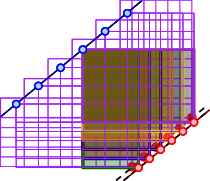
More surprisingly, this property extends, with a twist, to certain geometric range spaces that might have quadratic number of shallow ranges. Indeed, it is easy to show an example of points in the plane, where there are distinct rectangles, each one containing exactly two points, see Figure 1.2. However, one can “split” such ranges into a small number of canonical sets, such that the number of shallow sets in the canonical set system is near linear. This enables us to store the small canonical sets encountered during the scan explicitly in memory, and still use only near linear space.
We note that the idea of splitting ranges into small canonical ranges is an old idea in orthogonal range searching. It was used by Aronov et al. [AES10] for computing small -nets for these range spaces. The idea in the form we use, was further formalized by Ene et al. [EHR12].
Lower bounds. The lower bounds for multi-pass algorithms for the Set Cover problem are obtained via a careful reduction from Intersection Set Chasing. The latter problem is a communication complexity problem where players need to solve a certain “set-disjointness-like” problem in rounds. A recent paper [GO13] showed that this problem requires bits of communication complexity for rounds. This yields our desired trade-off of space in passes for exact protocols for Set Cover in the communication model and hence in the streaming model for . Furthermore, we show a stronger lower bound on memory space of sparse instances of Set Cover in which all input sets have cardinality at most . By a reduction from a variant of Equal Pointer Chasing which maps the problem to a sparse instance of Set Cover, we show that in order to have an exact streaming algorithm for -Sparse Set Cover with space, passes is necessary. More precisely, any -pass exact randomized algorithm for -Sparse Set Cover requires memory space, if and .
Our single pass lower bound proceeds by showing a lower bound for a one-way communication complexity problem in which one party (Alice) has a collection of sets, and the other party (Bob) needs to determine whether the complement of his set is covered by one of the Alice’s sets. We show that if Alice’s sets are chosen at random, then Bob can decode Alice’s input by employing a small collection of “query” sets. This implies that the amount of communication needed to solve the problem is linear in the description size of Alice’s sets, which is .
|
2 Streaming Algorithm for Set Cover
2.1 Algorithm
In this section, we design an efficient streaming algorithm for the Set Cover problem that matches the lower bound results we already know about the problem. In the Set Cover problem, for a given set system , the goal is to find a subset , such that covers and its cardinality is minimum. In the following, we sketch the iterSetCover algorithm (see also Figure 1.3).
In the iterSetCover algorithm, we have access to the algOfflineSC subroutine that solves the given Set Cover instance offline (using linear space) and returns a -approximate solution where could be anywhere between and depending on the computational model one assumes. Under exponential computational power, we can achieve the optimal cover of the given instance of the Set Cover (); however, under assumption, cannot be better than where is a constant [Fei98, RS97, AMS06, Mos12, DS14] given polynomial computational power.
Let be the initial number of elements in the given ground set. The iterSetCover algorithm, needs to guess (up to a factor of two) the size of the optimal cover of . To this end, the algorithm tries, in parallel, all values in . This step will only increase the memory space requirement by a factor of .
Consider the run of the iterSetCover algorithm, in which the guess is correct (i.e., , where OPT is an optimal solution). The idea is to go through iterations such that each iteration only makes two passes and at the end of each iteration the number of uncovered elements reduces by a factor of . Moreover, the algorithm is allowed to use space.
In each iteration, the algorithm starts with the current ground set of uncovered elements , and copies it to a leftover set . Let be a large enough uniform sample of elements . In a single pass, using , we estimate the size of all large sets in and add to the solution immediately (thus avoiding the need to store it in memory). Formally, if covers at least yet-uncovered elements of then it is a heavy set, and the algorithm immediately adds it to the output cover. Otherwise, if a set is small, i.e., its covers less than uncovered elements of , the algorithm stores the set in memory. Fortunately, it is enough to store its projection over the sampled elements explicitly (i.e., ) – this requires remembering only the indices of the elements of .
In order to show that a solution of the Set Cover problem over the sampled elements is a good cover of the initial Set Cover instance, we apply the relative ()-approximation sampling result of [HS11] (see Definition 2.4) and it is enough for to be of size . Using relative -approximation sampling, we show that after two passes the number of uncovered elements is reduced by a factor of . Note that the relative -approximation sampling improves over the Element Sampling technique used in [DIMV14] with respect to the number of passes.
Since in each iteration we pick sets and the number of uncovered elements decreases by a factor of , after iterations the algorithm picks sets and covers all elements. Moreover, the memory space of the whole algorithm is (see Lemma 2.2).
2.2 Analysis
In the rest of this section we prove that the iterSetCover algorithm with high probability returns a -approximate solution of Set Cover() in passes using memory space.
Lemma 2.1.
The number of passes the iterSetCover algorithm makes is .
Proof:
In each of the iterations of the iterSetCover algorithm, the algorithm makes two passes. In the first pass, based on the set of sampled elements , it decides whether to pick a set or keep its projection over (i.e., ) in the memory. Then the algorithm calls algOfflineSC which does not require any passes over . The second pass is for computing the set of uncovered elements at the end of the iteration. We need this pass because we only know the projection of the sets we picked in the current iteration over and not over the original set of uncovered elements. Thus, in total we make passes. Also note that for different guesses for the value of , we run the algorithm in parallel and hence the total number of passes remains .
Lemma 2.2.
The memory space used by the iterSetCover algorithm is .
Proof:
In each iteration of the algorithm, it picks during the first pass at most sets (more precisely at most sets) which requires memory. Moreover, in the first pass we keep the projection of the sets whose projection over the uncovered sampled elements has size at most . Since there are at most such sets, the total required space for storing the projections is bounded by
Since in the second pass the algorithm only updates the set of uncovered elements, the amount of space required in the second pass is . Thus, the total required space to perform each iteration of the iterSetCover algorithm is . Moreover, note that the algorithm does not need to keep the memory space used by the earlier iterations; thus, the total space consumed by the algorithm is .
Next we show the sets we picked before calling algOfflineSC has large size on .
Lemma 2.3.
With probability at least all sets that pass the “Size Test” in the iterSetCover algorithm have size at least .
Proof:
Let be a set of size less than . In expectation, is less than By Chernoff bound for large enough ,
Applying the union bound, with probability at least , all sets passing “Size Test” have size at least .
In what follows we define the relative -approximation sample of a set system and mention the result of Har-Peled and Sharir [HS11] on the minimum required number of sampled elements to get a relative -approximation of the given set system.
Definition 2.4.
Let be a set system, i.e., is a set of elements and is a family of subsets of the ground set . For given parameters , a subset is a relative -approximation for , if for each , we have that if then
If the range is light (i.e., ) then it is required that
Namely, is -multiplicative good estimator for the size of ranges that are at least -fraction of the ground set.
The following lemma is a simplified variant of a result in Har-Peled and Sharir [HS11] – indeed, a set system with sets, can have VC dimension at most . This simplified form also follows by a somewhat careful but straightforward application of Chernoff’s inequality.
Lemma 2.5.
Let be a finite set system, and be parameters. Then, a random sample of such that for an absolute constant is a relative -approximation, for all ranges in , with probability at least .
Lemma 2.6.
Assuming , after any iteration, with probability at least the number of uncovered elements decreases by a factor of , and this iteration adds sets to the output cover.
Proof:
Let be the set of uncovered elements at the beginning of the iteration and note that the total number of sets that is picked during the iteration is at most (see Lemma 2.3). Consider all possible such covers, that is , and observe that . Let be the collection that contains all possible sets of uncovered elements at the end of the iteration, defined as Moreover, set , and and note that . Since for large enough , by Lemma 2.5, is a relative -approximation of with probability. Let be the collection of sets picked during the iteration which covers all elements in . Since is a relative -approximation sample of with probability at least , the number of uncovered elements of (or ) by is at most .
Hence, in each iteration we pick sets and at the end of iteration the number of uncovered elements reduces by .
Lemma 2.7.
The iterSetCover algorithm computes a set cover of , whose size is within a factor of the size of an optimal cover with probability at least .
Proof:
Consider the run of iterSetCover for which the value of is between and . In each of the iterations made by the algorithm, by Lemma 2.6, the number of uncovered elements decreases by a factor of where is the number of initial elements to be covered by the sets. Moreover, the number of sets picked in each iteration is . Thus after iterations, all elements would be covered and the total number of sets in the solution is . Moreover by Lemma 2.6, the success probability of all the iterations, is at least .
Theorem 2.8.
The algorithm makes passes, uses memory space, and finds a -approximate solution of the Set Cover problem with high probability.
Furthermore, given enough number of passes the iterSetCover algorithm matches the known lower bound on the memory space of the streaming Set Cover problem up to a factor where is the number of sets in the input.
Proof:
As for the lower bound, note that by a result of Nisan [Nis02], any randomized ()-approximation protocol for Set Cover() in the one-way communication model requires bits of communication, no matter how many number of rounds it makes. This implies that any randomized -pass, ()-approximation algorithm for Set Cover() requires space, even under the exponential computational power assumption.
By the above, the iterSetCover algorithm makes passes and uses space to return a -approximate solution under the exponential computational power assumption (). Thus by letting , we will have a -approximation streaming algorithm using space which is optimal up to a factor of .
Theorem 2.8 provides a strong indication that our trade-off algorithm is optimal.
3 Lower Bound for Single Pass Algorithms
In this section, we study the Set Cover problem in the two-party communication model and give a tight lower bound on the communication complexity of the randomized protocols solving the problem in a single round. In the two-party Set Cover, we are given a set of elements and there are two players Alice and Bob where each of them has a collection of subsets of , and . The goal for them is to find a minimum size cover covering while communicating the fewest number of bits from Alice to Bob (In this model Alice communicates to Bob and then Bob should report a solution).
Our main lower bound result for the single pass protocols for Set Cover is the following theorem which implies that the naive approach in which one party sends all of its sets to the the other one is optimal.
Theorem 3.1.
Any single round randomized protocol that approximates Set Cover within a factor better than and error probability requires bits of communication where and and is a sufficiently large constant.
We consider the case in which the parties want to decide whether there exists a cover of size for in or not. If any of the parties has a cover of size at most for , then it becomes trivial. Thus the question is whether there exist and such that .
A key observation is that to decide whether there exist and such that , one can instead check whether there exists and such that . In other words we need to solve OR of a series of two-party Set Disjointness problems. In two-party Set Disjointness problem, Alice and Bob are given subsets of , and and the goal is to decide whether is empty or not with the fewest possible bits of communication. Set Disjointness is a well-studied problem in the communication complexity and it has been shown that any randomized protocol for Set Disjointness with error probability requires bits of communication where [BJKS04, KS92, Raz92].
We can think of the following extensions of the Set Disjointness problem.
-
Many vs One:
In this variant, Alice has subsets of , and Bob is given a single set . The goal is to determine whether there exists a set such that .
-
Many vs Many:
In this variant, each of Alice and Bob are given a collection of subsets of and the goal for them is to determine whether there exist and such that .
Note that deciding whether two-party Set Cover has a cover of size is equivalent to solving the (Many vs Many)-Set Disjointness problem. Moreover, any lower bound for (Many vs One)-Set Disjointness clearly implies the same lower bound for the (Many vs Many)-Set Disjointness problem. In the following theorem we show that any single-round randomized protocol that solves (Many vs One)-Set Disjointness() with error probability requires bits of communication.
Theorem 3.2.
Any randomized protocol for (Many vs One)-Set Disjointness with error probability that is requires bits of communication if where and are large enough constants.
The idea is to show that if there exists a single-round randomized protocol for the problem with bits of communication and error probability , then with constant probability one can distinguish distinct inputs using bits which is a contradiction.
Suppose that Alice has a collection of uniformly and independently random subsets of (in each of her subsets the probability that is in the subset is ). Lets assume that there exists a single round protocol for (Many vs One)-Set Disjointness() with error probability using bits of communication. Let algExistsDisj be Bob’s algorithm in protocol . Then we show that one can recover random bits with constant probability using algExistsDisj subroutine and the message sent by the first party in protocol . The algRecoverBit which is shown in Figure 3.1, is the algorithm to recover random bits using protocol and algExistsDisj.
To this end, Bob gets the message communicated by protocol from Alice and considers all subsets of size and of . Note that is communicated only once and thus the same is used for all queries that Bob makes. Then at each step Bob picks a random subset of size of and solve the (Many vs One)-Set Disjointness problem with input by running . Next we show that if is disjoint from a set in , then with high probability there is exactly one set in which is disjoint from (see Lemma 3.3). Thus once Bob finds out that his query, , is disjoint from a set in , he can query all sets and recover the set (or union of sets) in that is disjoint from . By a simple pruning step we can detect the ones that are union of more than one set in and only keep the sets in .
In Lemma 3.6, we show that the number of queries that Bob is required to make to recover is where is a constant.
algRecoverBit: for to do Let be a random subset of of size if // Discovering the set (or union of sets) // in disjoint from for if if s.t. // Pruning step , else if s.t. return
Lemma 3.3.
Let be a random subset of of size and let be a collection of m random subsets of . The probability that there exists exactly one set in that is disjoint from is at least .
Proof:
The probability that is disjoint from exactly one set in is
First we prove the first term in the above inequality. For an arbitrary set , since any element is contained in with probability , the probability that is disjoint from is .
Moreover since there exist pairs of sets in , and for each , the probability that and are disjoint from is ,
A family of sets is called intersecting if and only if for any sets either both and are non-empty or both and are empty; in other words, there exists no such that . Let be a collection of subsets of . We show that with high probability after testing queries for sufficiently large constant , the algRecoverBit algorithm recovers completely if is intersecting. First we show that with high probability the collection is intersecting.
Observation 3.4.
Let be a collection of uniformly random subsets of where . With probability at least , is an intersecting family.
Proof:
The probability that is and there are at most pairs of sets in . Thus with probability at least , is intersecting.
Observation 3.5.
The number of distinct inputs of Alice (collections of random subsets of ), that is distinguishable by algRecoverBit is .
Proof:
There are collections of random subsets of . By Observation 3.4, of them are intersecting. Since we can only recover the sets in the input collection and not their order, the distinct number of input collection that are distinguished by algRecoverBit is which is for .
By Observation 3.4 and only considering the case such that is intersecting, we have the following lemma.
Lemma 3.6.
Let be a collection of uniformly random subsets of and suppose that . After testing at most queries, with probability at least , is fully recovered, where is the success rate of protocol for the (Many vs One)-Set Disjointness problem.
Proof:
By Lemma 3.3, for each of size the probability that is disjoint from exactly one set in a random collection of sets is at least . Given is disjoint from exactly one set in , due to symmetry of the problem, the chance that is disjoint from a specific set is at least . After queries where is a large enough constant, for any , the probability that there is not a query that is only disjoint from is at most .
Thus after trying queries, with probability at least , for each we have at least one query that is only disjoint from (and not any other sets in ).
Once we have a query subset which is only disjoint from a single set , we can ask queries of size and recover . Note that if is disjoint from more than one sets in simultaneously, the process (asking queries of size ) will end up in recovering the union of those sets. Since is an intersecting family with high probability (Observation 3.4), by pruning step in the algRecoverBit algorithm we are guaranteed that at the end of the algorithm, what we returned is exactly . Moreover the total number of queries the algorithm makes is at most
for .
Thus after testing queries, will be recovered with probability at least where is the success probability of the protocol for (Many vs One)-Set Disjointness().
Corollary 3.7.
Let I be a protocol for (Many vs One)-Set Disjointness() with error probability and bits of communication such that for large enough . Then algRecoverBit recovers with constant success probability using bits of communication.
By Observation 3.5, since algRecoverBit distinguishes distinct inputs with constant probability of success (by Corollary 3.7), the size of message sent by Alice, should be . This proves Theorem 3.2.
Proof of
Theorem 3.1: As we showed earlier, the communication complexity of (Many vs One)-Set Disjointness is a lower bound for the communication complexity of Set Cover. Theorem 3.2 showed that any protocol for (Many vs One)-Set Disjointness with error probability less than requires bits of communication. Thus any single-round randomized protocol for Set Cover with error probability requires bits of communication.
Since any -pass streaming -approximation algorithm for problem P that uses memory space, is a -round two-party -approximation protocol for problem P using bits of communication [GM08], and by Theorem 3.1, we have the following lower bound for Set Cover problem in the streaming model.
Theorem 3.8.
Any single-pass randomized streaming algorithm for Set Cover() that computes a -approximate solution with probability requires memory space (assuming ).
4 Geometric Set Cover
In this section, we consider the streaming Set Cover problem in the geometric settings. We present an algorithm for the case where the elements are a set of points in the plane and the sets are either all disks, all axis-parallel rectangles, or all -fat triangles (which for simplicity we call shapes) given in a data stream. As before, the goal is to find the minimum size cover of points from the given sets. We call this problem the Points-Shapes Set Cover problem.
Note that, the description of each shape requires space and thus the Points-Shapes Set Cover problem is trivial to be solved in space. In this setting the goal is to design an algorithm whose space is sub-linear in . Here we show that almost the same algorithm as iterSetCover (with slight modifications) uses space to find an -approximate solution of the Points-Shapes Set Cover problem in constant passes.
4.1 Preliminaries
A triangle is called -fat (or simply fat) if the ratio between its longest edge and its height on this edge is bounded by a constant (there are several equivalent definitions of -fat triangles).
Definition 4.1.
Let be a set system such that is a set of points and is a collection of shapes, in the plane . The canonical representation of is a collection of regions such that the following conditions hold. First, each has description. Second, for each , there exists such that . Finally, for each , there exists sets such that for some constant .
Lemma 4.2.
(Lemma 4.18 in [EHR12]) Given a set of points in the plane and a parameter , one can compute a set of axis-parallel rectangles with the following property. For an arbitrary axis-parallel rectangle that contains at most points of , there exist two axis-parallel rectangles whose union has the same intersection with as , i.e., .
Lemma 4.3.
(Theorem 5.6 in [EHR12]) Given a set of points in , a parameter and a constant , one can compute a set of regions each having description with the following property. For an arbitrary -fat triangle that contains at most points of , there exist nine regions from whose union has the same intersection with as .
Using the above lemmas we get the following lemma.
Lemma 4.4.
Let be a set of points in and let be a set of shapes (discs, axis-parallel rectangles or fat triangles), such that each set in contains at most points of . Then, in a single pass over the stream of sets , one can compute the canonical representation of . Moreover, the size of the canonical representation is at most and the space requirement of the algorithm is .
Proof:
For the case of axis-parallel rectangles and fat triangles, first we use Lemma 4.2 and Lemma 4.3 to get the set offline which require memory space. Then by making one pass over the stream of sets , we can find the canonical representation by picking all the sets such that for some . For discs however, we just make one pass over the sets and keep a maximal subset such that for each pair of sets their projection on are different, i.e., . By a standard technique of Clarkson and Shor [CS89], it can be proved that the size of the canonical representation, i.e., , is bounded by . Note that this is just counting the number of discs that contain at most points, namely the at most -level discs.
4.2 Algorithm
The outline of the Points-Shapes-Set-Cover algorithm (shown in Figure 4.1) is very similar to the iterSetCover algorithm presented earlier in Section 2.
In the first pass, the algorithm picks all the sets that cover a large number of yet-uncovered elements. Next, we sample . Since we have removed all the ranges that have large size, in the first pass, the size of the remaining ranges restricted to the sample is small. Therefore by Lemma 4.4, the canonical representation of has small size and we can afford to store it in the memory. We use Lemma 4.4 to compute the canonical representation in one pass. The algorithm then uses the sets in to find a cover for the points of . Next, in one additional pass, the algorithm replaces each set in by one of its supersets in .
Finally, note that in the algorithm of Section 2, we are assuming that the size of the optimal solution is . Thus it is enough to stop the iterations once the number of uncovered elements is less than . Then we can pick an arbitrary set for each of the uncovered elements. This would add only more sets to the solution. Using this idea, we can reduce the size of the sampled elements down to which would help us in getting near-linear space in the geometric setting. Note that the final pass of the algorithm can be embedded into the previous passes but for the sake of clarity we write it separately.
algGeomSC: for do in parallel: // Let and Repeat times: for do // Pass if then sample of of size compCanonicalRep // Pass algOfflineSC() for do // Pass if s.t. then for do // Final Pass if then return smallest computed in parallel
4.3 Analysis
By a similar approach to what we used in Section 2 to analyze the pass count and approximation guarantee of iterSetCover algorithm, we can show that the number of passes of the algGeomSC algorithm is (which can be reduced to with minor changes), and the algorithm returns an -approximate solution. Next, we analyze the space usage and the correctness of the algorithm. Note that our analysis in this section only works for .
Lemma 4.5.
The algorithm uses space.
Proof:
Consider an iteration of the algorithm. The memory space used in the first pass of each iteration is . The size of is and after the first pass the size of each set is at most . Thus using Chernoff bound for each set ,
Thus, with probability at least (by the union bound), all the sets that are not picked in the first pass, cover at most elements of . Therefore, we can use Lemma 4.4 to show that the number of sets in the canonical representation of is at most
as long as . To store each set in a canonical representation of only constant space is required. Moreover, by Lemma 4.4, the space requirement of the second pass is . Therefore, the total required space is and the lemma follows.
Theorem 4.6.
Given a set system defined over a set of points in the plane, and a set of ranges (which are either all disks, axis-parallel rectangles, or fat triangles). Let be the quality of approximation to the offline set-cover solver we have, and let be an arbitrary parameter.
Setting , the algorithm algGeomSC, depicted in Figure 4.1, with high probability, returns an -approximate solution of the optimal set cover solution for the instance . This algorithm uses space, and performs constant passes over the data.
Proof:
As before consider the run of the algorithm in which . Let be the set of uncovered elements at the beginning of the iteration and note that the total number of sets that is picked during the iteration is at most where is the constant defined in Definition 4.1. Let denote all possible such covers, that is . Let be the collection that contains all possible set of uncovered elements at the end of the iteration, defined as . Set , and . Since for large enough , with probability at least , by Lemma 2.5, the set of sampled elements is a relative -approximation sample of .
Let be the collection of sets picked in the third pass of the algorithm that covers all elements in . By Lemma 4.4, for some constant . Since with high probability is a relative -approximation sample of , the number of uncovered elements of (or ) after adding to is at most . Thus with probability at least , in each iteration and by adding sets, the number of uncovered elements reduces by a factor of .
Therefore, after iterations (for ) the algorithm picks sets and with high probability the number of uncovered elements is at most . Thus, in the final pass the algorithm only adds sets to the solution , and hence the approximation factor of the algorithm is .
Remark 4.7.
The result of Theorem 4.6 is similar to the result of Agarwal and Pan [AP14] – except that their algorithm performs iterations over the data, while the algorithm of Theorem 4.6 performs only a constant number of iterations. In particular, one can use the algorithm of Agarwal and Pan [AP14] as the offline solver.
5 Lower bound for multipass algorithms
In this section we give lower bound on the memory space of multipass streaming algorithms for the Set Cover problem. Our main result is space for streaming algorithms that return an optimal solution of the Set Cover problem in passes for . Our approach is to reduce the communication Intersection Set Chasing() problem introduced by Guruswami and Onak [GO13] to the communication Set Cover problem.
Consider a communication problem with players . The problem is a -communication problem if players communicate in rounds and in each round they speak in order . At the end of the th round should return the solution. Moreover we assume private randomness and public messages. In what follows we define the communication Set Chasing and Intersection Set Chasing problems.
Definition 5.1 (Communication Set Chasing Problem).
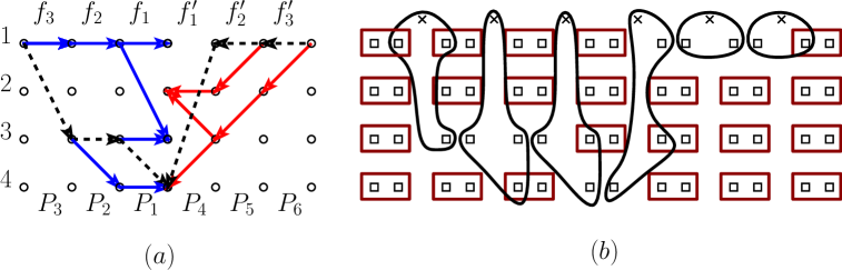
The Set Chasing() problem is a communication problem in which the player has a function and the goal is to compute where . Figure 5.1(a) shows an instance of the communication Set Chasing ().
Definition 5.2 (Communication Intersection Set Chasing).
The Intersection Set Chasing() is a communication problem in which the first players have an instance of the Set Chasing() problem and the other players have another instance of the Set Chasing() problem. The output of the Intersection Set Chasing() is if the solutions of the two instances of the Set Chasing() intersect and otherwise. Figure 5.1(b) shows an instance of the Intersection Set Chasing (). The function of each player is specified by a set of directed edges form a copy of vertices labeled to another copy of vertices labeled .
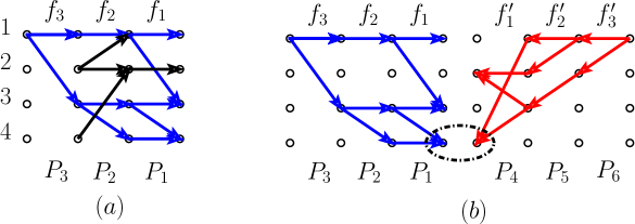
The communication Set Chasing problem is a generalization of the well-known communication Pointer Chasing problem in which player has a function and the goal is to compute .
[GO13] showed that any randomized protocol that solves Intersection Set Chasing() with error probability less than , requires bits of communication where is sufficiently large and . In Theorem 5.4, we reduce the communication Intersection Set Chasing problem to the communication Set Cover problem and then give the first superlinear memory lower bound for the streaming Set Cover problem.
Definition 5.3 (Communication Set Cover() Problem).
The communication Set Cover() is a communication problem in which a collection of elements is given to all players and each player has a collection of subsets of , . The goal is to solve Set Cover() using the minimum number of communication bits.
Theorem 5.4.
Any passes streaming algorithm that solves the Set Cover() optimally with constant probability of error requires memory space where and .
Consider an instance of the communication Intersection Set Chasing(). We construct an instance of the communication Set Cover() problem such that solving Set Cover() optimally determines whether the output of is or not.
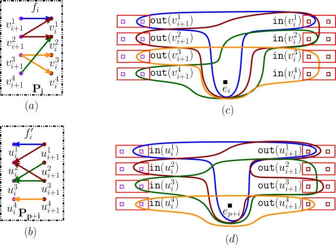
The instance consists of players. Each player has a function and each player has a function (see Figure 5.1). In , each function is shown by a set of vertices and such that there is a directed edge from to if and only if . Similarly, each function is denoted by a set of vertices and such that there is a directed edge from to if and only if (see Figure 5.2(a) and Figure 5.2(b)).
In the corresponding communication Set Cover instance of , we add two elements and per each vertex where . We also add two elements and per each vertex where . In addition to these elements, for each player , we add an element (see Figure 5.2(c) and Figure 5.2(d)).
Next, we define a collection of sets in the corresponding Set Cover instance of . For each player , where , we add a single set containing and for all out-going edges . Moreover, all sets contain the element . Next, for each vertex we add a set that contains the two corresponding elements of , and . In Figure 5.2(c), the red rectangles denote -type sets and the curves denote -type sets for the first half of the players.
Similarly to the sets corresponding to players to , for each player where , we add a set containing and for all in-coming edges of (denoting ). The set contains the element too. Next, for each vertex we add a set that contains the two corresponding elements of , and . In Figure 5.2(d), the red rectangles denote -type sets and the curves denote -type sets for the second half of the players.
At the end, we merge s and s as shown in Figure 5.3. After merging the corresponding sets of s () and the corresponding sets of s ( ), we call the merged sets .
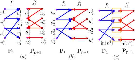
The main claim is that if the solution of is then the size of an optimal solution of its corresponding Set Cover instance is ; otherwise, it is .
Lemma 5.5.
The size of any feasible solution of is at least .
Proof:
For each player (), since s are only covered by and , at least sets are required to cover . Moreover for player , since s are only covered by and is only covered by , all sets must be selected in any feasible solution of .
Similarly for each player (), since in()s are only covered by and , at least sets are required to cover . Moreover, considering , since is only covered by , all sets must be selected in any feasible solution of .
All together, at least sets should be selected in any feasible solution of .
Lemma 5.6.
Suppose that the solution of is . Then the size of an optimal solution of its corresponding Set Cover instance is exactly .
Proof:
By Lemma 5.5, the size of an optimal solution of is at least . Here we prove that sets suffice when the solution of is . Let be a path in such that (since the solution of is such a path exists). The corresponding solution to can be constructed as follows (See Figure 5.4):
-
•
Pick and all s ( sets).
-
•
For each in where , pick the set in the solution. Moreover, for each such pick all sets where ( sets).
-
•
For (or ), pick the set . Moreover, pick all sets where ( sets).
-
•
For each in where , pick the set in the solution. Moreover, for each such pick all sets where ( sets).
-
•
Pick all s ( sets).
It is straightforward to see that the solution constructed above is a feasible solution.
Lemma 5.7.
Suppose that the size of an optimal solution of the corresponding Set Cover instance of , , is . Then the solution of is .
Proof:
As we proved earlier in Lemma 5.5, any feasible solution of picks and . Moreover, we proved that for each , at least sets should be selected from . Similarly, for each , at least sets should be selected from , . Thus if a feasible solution of , OPT, is of size , it has exactly sets from each specified group.
Next we consider the first half of the players and second half of the players separately. Consider such that . Let be the sets picked in the optimal solution (because of there should be at least one set of form in OPT). Since each is only covered by and , for all , should be selected in OPT. Moreover, for all , should not be contained in OPT (otherwise the size of OPT would be larger than ). Consider . Since is not in OPT, there should be a set selected in OPT such that is contained in . Thus by considering s in a decreasing order and using induction, if is in OPT then is reachable form .
Next consider a set that is selected in OPT (). By similar argument, is not in OPT and there exists a set (or if ) in OPT such that is contained in . Let be the set of vertices whose corresponding elements are in . Then by induction, there exists an index such that is reachable from and is also reachable from all . Moreover, the way we constructed the instance guarantees that all sets contains . Hence if the size of an optimal solution of is then the solution of is .
Corollary 5.8.
Intersection Set Chasing() returns if and only if the size of optimal solution of its corresponding Set Cover instance (as described here) is .
Observation 5.9.
Any streaming algorithm for Set Cover, , that in passes solves the problem optimally with a probability of error and consumes memory space, solves the corresponding communication Set Cover problem in rounds using bits of communication with probability error .
Proof:
Starting from player , each player runs over its input sets and once is done with its input, she sends the working memory of publicly to other players. Then next player starts the same routine using the state of the working memory received from the previous player. Since solves the Set Cover instance optimally after passes using space with probability error , applying as a black box we can solve in rounds using bits of communication with probability error .
Proof of
Theorem 5.4: By Observation 5.9, any -round -space algorithm that solves streaming Set Cover () optimally can be used to solve the communication Set Cover() problem in rounds using bits of communication. Moreover, by Corollary 5.8, we can decide the solution of the communication Intersection Set Chasing() by solving its corresponding communication Set Cover problem. Note that while working with the corresponding Set Cover instance of Intersection Set Chasing(), all players know the collection of elements and each player can construct its collection of sets using (or ).
However, by a result of [GO13], we know that any protocol that solves the communication Intersection Set Chasing() problem with probability of error less than , requires bits of communication. Since in the corresponding Set Cover instance of the communication Intersection Set Chasing(), and , any )-pass streaming algorithm that solves the Set Cover problem optimally with a probability of error at most , requires bits of communication. Then using Observation 5.9, since , any -pass streaming algorithmof Set Cover that finds an optimal solution with error probability less than , requires space.
6 Lower Boundfor Sparse Set Cover in Multiple Passes
In this part we give a stronger lower bound for the instances of the streaming Set Cover problem with sparse input sets. An instance of the Set Cover problem is -Sparse Set Cover, if for each set we have . We can us the same reduction approach described earlier in Section 5 to show that any -pass streaming algorithm for -Sparse Set Cover requires memory space if and . To prove this, we need to explain more details of the approach of [GO13] on the lower bound of the communication Intersection Set Chasing problem. They first obtained a lower bound for Equal Pointer Chasing() problem in which two instances of the communication Pointer Chasing() are given and the goal is to decide whether these two instances point to a same value or not; .
Definition 6.1 (-non-injective functions).
A function is called -non-injective if there exists of size at least and such that for all , .
Definition 6.2 (Pointer Chasing Problem).
Pointer Chasing() is a communication problem in which the player has a function and the goal is to compute .
Definition 6.3 (Equal Limited Pointer Chasing Problem).
Equal Pointer Chasing() is a communication problem in which the first players have an instance of the Pointer Chasing() problem and the other players have another instance of the Pointer Chasing() problem. The output of the Equal Pointer Chasing() is if the solutions of the two instances of Pointer Chasing() have the same value and otherwise. Furthermore in another variant of pointer chasing problem, Equal Limited Pointer Chasing(), if there exists -non-injective function , then the output is . Otherwise, the output is the same as the value in Equal Pointer Chasing().
For a boolean communication problem P, (P) is defined to be of instances of P and the output of (P) is if and only if the output of any of the instances is . Using a direct sum argument, [GO13] showed that the communication complexity of (Equal Limited Pointer Chasing()) is times the communication complexity of Equal Limited Pointer Chasing().
Lemma 6.4 ([GO13]).
Let , , and be positive integers such that , and . Then the amount of bits of communication to solve (Equal Limited Pointer Chasing()) with error probability less than is .
Lemma 6.5 ([GO13]).
Let , , and be positive integers such that . Then if there is a protocol that solves Intersection Set Chasing() with probability of error less than using bits of communication, there is a protocol that solves (Equal Limited Pointer Chasing()) with probability of error at most using bits of communication.
Consider an instance of (Equal Limited Pointer Chasing ()) in which where . By Lemma 6.4, the required amount of bits of communication to solve the instance with constant success probability is . Then,applying Lemma 6.5, to solve the corresponding Intersection Set Chasing, bits of communication is required.
In the reduction from (Equal Limited Pointer Chasing()) to Intersection Set Chasing() (proof of Lemma 6.5), the -non-injective property is preserved. In other words, in the corresponding Intersection Set Chasing instance each player’s functions is union of -non-injective functions 666The Intersection Set Chasing instance is obtained by overlaying the instances of Equal Pointer Chasing(). To be more precise, the function of player in instance is ( are randomly chosen permutation functions) and then stack the functions on top of each other.. Given that none of the functions is -non-injective, the corresponding Set Cover instance will have sets of size at most (-type sets are of size at most for and of size at most for ). Since , the corresponding Set Cover instance is -sparse. As we showed earlier in the reduction from Intersection Set Chasing to Set Cover, the number of elements (and sets) in the corresponding Set Cover instance is . Thus we have the following result for -Sparse Set Cover problem.
Theorem 6.6.
For , any streaming algorithm that solves -Sparse Set Cover() optimally with probability of error less than in passes requires memory space for .
References
- [AES10] B. Aronov, E. Ezra, and M. Sharir. Small-size -nets for axis-parallel rectangles and boxes. SIAM Journal on Computing, 39(7):3248–3282, 2010.
- [AKL16] S. Assadi, S. Khanna, and Y. Li. Tight bounds for single-pass streaming complexity of the set cover problem. In Proc. 48th Annu. ACM Sympos. Theory Comput. (STOC), 2016.
- [AMS06] N. Alon, D. Moshkovitz, and S. Safra. Algorithmic construction of sets for -restrictions. ACM Trans. Algo., 2(2):153–177, 2006.
- [AP14] P. K. Agarwal and J. Pan. Near-linear algorithms for geometric hitting sets and set covers. In Proc. 30th Annu. Sympos. Comput. Geom. (SoCG), pages 271–279, 2014.
- [BJKS04] Z. Bar-Yossef, T. S. Jayram, R. Kumar, and D. Sivakumar. An information statistics approach to data stream and communication complexity. J. Comput. Sys. Sci., 68(4):702–732, 2004.
- [CKT10] F. Chierichetti, R. Kumar, and A. Tomkins. Max-cover in map-reduce. In Proc. 19th Int. Conf. World Wide Web (WWW), pages 231–240, 2010.
- [CKW10] G. Cormode, H. J. Karloff, and A. Wirth. Set cover algorithms for very large datasets. In Proc. 19th ACM Conf. Info. Know. Manag. (CIKM), pages 479–488, 2010.
- [CS89] K. L. Clarkson and P. W. Shor. Applications of random sampling in computational geometry, II. Discrete Comput. Geom., 4:387–421, 1989.
- [CV07] K. L. Clarkson and K. Varadarajan. Improved approximation algorithms for geometric set cover. Discrete Comput. Geom., 37(1):43–58, 2007.
- [CW16] A. Chakrabarti and A. Wirth. Incidence geometries and the pass complexity of semi-streaming set cover. In Proc. 27th ACM-SIAM Sympos. Discrete Algs. (SODA), pages 1365–1373, 2016.
- [DIMV14] E. D. Demaine, P. Indyk, S. Mahabadi, and A. Vakilian. On streaming and communication complexity of the set cover problem. In Proc. 28th Int. Symp. Dist. Comp. (DISC), volume 8784 of Lect. Notes in Comp. Sci., pages 484–498, 2014.
- [DS14] I. Dinur and D. Steurer. Analytical approach to parallel repetition. In Proc. 46th Annu. ACM Sympos. Theory Comput. (STOC), pages 624–633. ACM, 2014.
- [EHR12] A. Ene, S. Har-Peled, and B. Raichel. Geometric packing under non-uniform constraints. In Proc. 28th Annu. Sympos. Comput. Geom. (SoCG), pages 11–20, 2012.
- [ER14] Y. Emek and A. Rosén. Semi-streaming set cover. In Proc. 41st Int. Colloq. Automata Lang. Prog. (ICALP), volume 8572 of Lect. Notes in Comp. Sci., pages 453–464, 2014.
- [Fei98] U. Feige. A threshold of ln n for approximating set cover. Journal of the ACM (JACM), 45(4):634–652, 1998.
- [FG88] T. Feder and D. H. Greene. Optimal algorithms for approximate clustering. In Proc. 20th Annu. ACM Sympos. Theory Comput. (STOC), pages 434–444, 1988.
- [FPT81] R. J. Fowler, M. S. Paterson, and S. L. Tanimoto. Optimal packing and covering in the plane are NP-complete. Inform. Process. Lett., 12(3):133–137, 1981.
- [GM07] S. Guha and A. McGregor. Lower bounds for quantile estimation in random-order and multi-pass streaming. In Proc. 34th Int. Colloq. Automata Lang. Prog. (ICALP), volume 4596 of Lect. Notes in Comp. Sci., pages 704–715, 2007.
- [GM08] S. Guha and A. McGregor. Tight lower bounds for multi-pass stream computation via pass elimination. In Proc. 35th Int. Colloq. Automata Lang. Prog. (ICALP), volume 5125 of Lect. Notes in Comp. Sci., pages 760–772, 2008.
- [GO13] V. Guruswami and K. Onak. Superlinear lower bounds for multipass graph processing. In Proc. 28th Conf. Comput. Complexity (CCC), pages 287–298, 2013.
- [GW97] T. Grossman and A. Wool. Computational experience with approximation algorithms for the set covering problem. Euro. J. Oper. Res., 101(1):81–92, 1997.
- [HQ15] S. Har-Peled and K. Quanrud. Approximation algorithms for polynomial-expansion and low-density graphs. In Proc. 23nd Annu. European Sympos. Algorithms (ESA), volume 9294 of Lect. Notes in Comp. Sci., pages 717–728, 2015.
- [HS11] S. Har-Peled and M. Sharir. Relative -approximations in geometry. Discrete Comput. Geom., 45(3):462–496, 2011.
- [KMVV13] R. Kumar, B. Moseley, S. Vassilvitskii, and A. Vattani. Fast greedy algorithms in MapReduce and streaming. In Proc. 25th ACM Sympos. Parallel Alg. Arch. (SPAA), pages 1–10, 2013.
- [KS92] B. Kalyanasundaram and G. Schintger. The probabilistic communication complexity of set intersection. SIAM J. Discrete Math., 5(4):545–557, 1992.
- [Mos12] D. Moshkovitz. The projection games conjecture and the NP-hardness of -approximating set-cover. In Approximation, Randomization, and Combinatorial Optimization. Algorithms and Techniques, pages 276–287. Springer, 2012.
- [MRR14] N. H. Mustafa, R. Raman, and S. Ray. Settling the apx-hardness status for geometric set cover. In Proc. 55th Annu. IEEE Sympos. Found. Comput. Sci. (FOCS), pages 541–550, 2014.
- [Nis02] N. Nisan. The communication complexity of approximate set packing and covering. In Proc. 29th Int. Colloq. Automata Lang. Prog. (ICALP), pages 868–875, 2002.
- [Raz92] A. A. Razborov. On the distributional complexity of disjointness. Theo. Comp. Sci., 106(2):385–390, 1992.
- [RS97] R. Raz and S. Safra. A sub-constant error-probability low-degree test, and a sub-constant error-probability PCP characterization of NP. In Proc. 29th Annu. ACM Sympos. Theory Comput. (STOC), pages 475–484, 1997.
- [SG09] B. Saha and L. Getoor. On maximum coverage in the streaming model & application to multi-topic blog-watch. In Proc. SIAM Int. Conf. Data Mining (SDM), pages 697–708, 2009.