A maximum principle for diffusive Lotka-Volterra systems of two competing species

Abstract

Using an elementary approach, we establish a new maximum principle for the diffusive Lotka-Volterra system of two competing species, which involves pointwise estimate of an elliptic equation consisting of the second derivative of one function, the first derivative of another function, and a quadratic nonlinearity. This maximum principle gives a priori estimates for the total mass of the two species. Moreover, applying it to the system of three competing species leads to a nonexistence theorem of traveling wave solutions.

1 Introduction

In this paper we study the following diffusive Lotka-Volterra system of two competing species:

$$\begin{cases}u_{t}=d_{1}\,u_{yy}+u\,(\sigma_{1}-c_{11}\,u-c_{12}\,v),\quad y\in\mathbb{R},\quad t>0,\\ \\ \hskip 1.99168ptv_{t}=d_{2}\,v_{yy}+v\,(\sigma_{2}-c_{21}\,u-c_{22}\,v),\quad y\in\mathbb{R},\quad t>0,\\ \end{cases}$$ (1.1)

which is a system frequently used to model competitive behaviour between two distinct species. Here $u(y,t)$ and $v(y,t)$ stand for the density of the two species $u$ and $v$, respectively; $d_{i}$, $\sigma_{i}$, $c_{ii}$ $(i=1,2)$, and $c_{ij}$ $(i,j=1,2\ \text{with}\;i\neq j)$ are the respective diffusion rates, intrinsic growth rates, intra-specific competition rates, and inter-specific competition rates, all of which are assumed to be positive. The problem as to which species will survive in a competitive system is of importance in ecology. In order to tackle this problem, we consider traveling wave solutions, which are solutions of the form

$$(u(y,t),v(y,t))=(u(x),v(x)),\quad x=y-\theta\,t,$$ (1.2)

where $\theta$ is the propagation speed of the traveling wave. In general, the sign of $\theta$ indicates which species is stronger and can survive.

We note that by using a suitable scaling, the two-species system (1.1) can be rewritten as

$$\begin{cases}u_{t}=\;\;u_{yy}+\;\;u\,(1-u-a_{1}\,v),\quad y\in\mathbb{R},\quad t>0,\\ \\ v_{t}=d\,v_{yy}+k\,v\,(1-a_{2}\,u-v),\quad y\in\mathbb{R},\quad t>0,\\ \end{cases}$$ (1.3)

where $d$, $k$, $a_{1}$ and $a_{2}$ are positive parameters. It is readily seen that in general, (1.3) has four equilibria: $\textbf{e}_{1}=(0,0)$, $\textbf{e}_{2}=(1,0)$, $\textbf{e}_{3}=(0,1)$ and $\textbf{e}_{4}=(u^{\ast},v^{\ast})$, where $(u^{\ast},v^{\ast})=(\frac{1-a_{1}}{1-a_{1}\,a_{2}},\frac{1-a_{2}}{1-a_{1}\,a_{2}})$ is the intersection of the two straight lines $1-u-a_{1}\,v=0$ and $1-a_{2}\,u-v=0$, whenever it exists. We note that $u^{\ast},v^{\ast}>0$ if and only if $a_{1},a_{2}<1$ or $a_{1},a_{2}>1$. When the domain is bounded, the asymptotic behavior of solutions $(u(y,t),v(y,t))$ for (1.3) with initial conditions $u(y,0),v(y,0)>0$ can be classified into four cases, as described in:

Proposition A ([3]).

Let $(u(y,t),v(y,t))$ be the solution of (1.3) with the entire space $\mathbb{R}$ replaced by a bounded domain in $\mathbb{R}$ under the zero Neumann boundary conditions. Then for initial conditions $u(x,0)$,$v(x,0)>0$, we have

• $a_{1}<1<a_{2}$        $\Rightarrow$ $\lim\limits_{t\rightarrow\infty}(u(y,t),v(y,t))=(1,0)$;

• $a_{2}<1<a_{1}$        $\Rightarrow$ $\lim\limits_{t\rightarrow\infty}(u(y,t),v(y,t))=(0,1)$;

• $a_{1}>1,a_{2}>1$      $\Rightarrow$ $(1,0)$ and $(0,1)$ are locally stable equilibria;

• $a_{1}<1,a_{2}<1$      $\Rightarrow$ $\lim\limits_{t\rightarrow\infty}(u(y,t),v(y,t))=(u^{\ast},v^{\ast})$.

In this paper, we consider the following traveling wave problems, which are obtained by substituting (1.2) into (1.3) and into (1.1) respectively,

$$\begin{cases}\vspace{3mm}\hskip 5.69054ptu_{xx}+\theta\,u_{x}+\;\;u\,(1-u-a_{1}\,v)=0,\quad x\in\mathbb{R},\\ \vspace{3mm}d\,v_{xx}+\theta\,v_{x}+k\,v\,(1-a_{2}\,u-v)=0,\quad x\in\mathbb{R},\\ (u,v)(-\infty)=\text{\bf e}_{2},\quad(u,v)(+\infty)=\text{\bf e}_{3},\end{cases}$$ (1.4)

and

$$\begin{cases}\vspace{3mm}d_{1}\,u_{xx}+\theta\,u_{x}+u\,(\sigma_{1}-c_{11}\,u-c_{12}\,v)=0,\quad x\in\mathbb{R},\\ \vspace{3mm}d_{2}\,v_{xx}\hskip 2.27621pt+\theta\,v_{x}+v\,(\sigma_{2}-c_{21}\,u-c_{22}\,v)=0,\quad x\in\mathbb{R},\\ (u,v)(-\infty)=\big{(}\frac{\displaystyle\sigma_{1}}{\displaystyle c_{11}},0\big{)},\quad(u,v)(+\infty)=\big{(}0,\frac{\displaystyle\sigma_{2}}{\displaystyle c_{22}}\big{)}.\end{cases}$$ (1.5)

We call a solution $(u(x),v(x))$ of (1.4) an $(\textbf{e}_{2},\textbf{e}_{3})$-wave. The typical situation

$$\lim_{x\to-\infty}(u,v)(x)=(1,0),\;\lim_{x\to\infty}(u,v)(x)=(0,1),$$ (1.6)

i.e. $u$ is dominant on the left region and $v$ is dominant on the right region of $\mathbb{R}$, motivates us to study the $(\textbf{e}_{2},\textbf{e}_{3})$-wave. In this situation, $u$ will occupy the whole domain eventually if $\theta>0$ while $v$ will occupy the whole domain eventually if $\theta<0$. From the viewpoint of ecology, we can conclude that the sign of $\theta$ determines which species is stronger, i.e. $u$ is stronger if $\theta>0$ and $v$ is stronger if $\theta<0$.

Much attention has been paid to the $(\textbf{e}_{2},\textbf{e}_{3})$-wave. For cases $(\textit{i})$ or $(\textit{iii})$ in Proposition A, Kan-on ([6],[7]), Fei and Carr ([4]), Leung, Hou and Li ([9]), and Leung and Feng ([8]) established the existence of $(\textbf{e}_{2},\textbf{e}_{3})$-waves employing different approaches. Under certain assumptions on the parameters, Mimura and Rodrigo ([10, 11]) constructed exact $(\textbf{e}_{2},\textbf{e}_{3})$-waves by applying a judicious ansätz for solutions. By applying the hyperbolic tangent method, Hung([5]) found exact $(\textbf{e}_{2},\textbf{e}_{3})$-waves under certain assumptions on the parameters. All the exact $(\textbf{e}_{2},\textbf{e}_{3})$-waves proposed by Mimura and Rodrigo ([10, 11]) and Hung([5]) are represented in terms of polynomials in hyperbolic tangent functions. Throughout this paper, we restrict our attention to the bistable case, i.e. case $(\textit{iii})$ $a_{1}>1,a_{2}>1$ in Proposition A.

To understand the ecological capacity of the inhabitant of the two competing species, the investigation of the total mass or the total density of the two species $u$ and $v$ is essential since the inhabitant is resource-limited. This gives rises to the problem as to the estimate of $u+v$ in (1.5). In [1], upper and lower bounds of $u+v$ are given when the two diffusion rates $d_{1}$ and $d_{2}$ are equal. However, the approach employed in [1] to obtain upper or lower bounds for $u+v$ cannot be applied to the case where the diffusion rates $d_{1}$ and $d_{2}$ are not equal.

The above discussion raises the following questions:

Q1: In (1.5), when $d_{1}\neq d_{2}$, can upper and lower bounds of $u+v$ be obtained?

As for the answer to Q1, it seems as far as we know, not available in the literature. To give an affirmative answer to this question, we develop a new but elementary approach. In fact, employing this approach leads to an affirmative answer to the following more general question:

Q2: In (1.5), when $d_{1}\neq d_{2}$, can upper and lower bounds of $\tau_{1}\,u+\tau_{2}\,v$, where $\tau_{1},\tau_{2}>0$ are arbitrary constants, be given?

Since the physical units of $u$ and $v$ may not be identical, it makes sense to consider $\tau_{1}\,u+\tau_{2}\,v$ for the total mass in general. Although we can estimate $\tau_{1}\,u+\tau_{2}\,v$ via

$$\min[\tau_{1},\tau_{2}]\,(u+v)\leq\tau_{1}\,u+\tau_{2}\,v\leq\max[\tau_{1},\tau_{2}]\,(u+v)$$ (1.7)

once $u+v$ is measured, more information will be wasted in this manner of estimation as the difference of $\tau_{1}$ and $\tau_{2}$ becomes larger. Consequently, an approach which can accommodate to various $\tau_{1}$ and $\tau_{2}$ will be of great interest.

By adding the two equations in (1.5), we obtain an equation involving $p(x)=\alpha\,u+\beta\,v$ and $q(x)=d_{1}\,\alpha\,u+d_{2}\,\beta\,v$

$$0 =\alpha\,\big{(}d_{1}\,u_{xx}+\theta\,u_{x}+u\,(\sigma_{1}-c_{11}\,u-c_{12}\,v)\big{)}+\beta\,\big{(}d_{2}\,v_{xx}+\theta\,v_{x}+v\,(\sigma_{2}-c_{21}\,u-c_{22}\,v)\big{)}$$

$$=q^{\prime\prime}(x)+\theta\,p^{\prime}(x)+\alpha\,u\,(\sigma_{1}-c_{11}\,u-c_{12}\,v)+\beta\,v\,(\sigma_{2}-c_{21}\,u-c_{22}\,v).$$

The case where $d_{1}=d_{2}$ or $p(x)$ is a constant multiple of $q(x)$ has been considered in [1]. Obviously, difficulties arise, and the approach used in [1] cannot be applied when $d_{1}\neq d_{2}$ since $p(x)$ no longer can be written as a constant multiple of $q(x)$. The approach proposed here can be employed to give estimates of $q(x)$ even distinct $p(x)$ and $q(x)$ (i.e. $d_{1}\neq d_{2}$) are involved in the scalar equation (3).

To simplify the problem, we consider (1.4) first and present the results for (1.5) in Section 6. One of the main results in this paper is the following maximum principle for Lotka-Volterra systems of two strongly competing species.

Theorem 1.1 (Maximum Principle for $q(x)$).

Suppose that $a_{1}>1,a_{2}>1$ and $(u(x),v(x))$ is a nonnegative solution to (1.4). Then

$$\min\Big{[}\frac{\alpha}{a_{2}\,d},\frac{\beta}{a_{1}}\Big{]}\min[1,d^{2}]\leq q(x)\leq\max\Big{[}\frac{\alpha}{d},\beta\Big{]}\max[1,d^{2}]\ \text{ for }x\in\mathbb{R},$$ (1.9)

where $q(x)=\alpha\,u(x)+d\,\beta\,v(x)$ and $\alpha$, $\beta$ are arbitrary positive constants.

In particular, we notice that the estimate of $q$ in Theorem 1.1 does not depend on the propagating speed $\theta$ and the constant $k$.

The maximum principle in Theorem 1.1 can be generalized to hold true for a wider class of autonomous elliptic systems:

$$\begin{cases}\vspace{3mm}d_{1}\,u_{xx}+\theta\,u_{x}+u^{m}\,f(u,v)=0,\quad x\in\mathbb{R},\\ \vspace{3mm}d_{2}\,v_{xx}\hskip 2.27621pt+\theta\,v_{x}+v^{n}\,g(u,v)=0,\quad x\in\mathbb{R},\\ (u,v)(-\infty)=\text{\bf e}_{-},\quad(u,v)(+\infty)=\text{\bf e}_{+},\end{cases}$$ (1.10)

where $m\geq 0$, $n\geq 0$ and

$$\text{\bf e}_{-},\text{\bf e}_{+}\in\mathcal{C}_{f,g}=\{(u,v)\;|\;u^{m}f(u,v)=0,v^{n}g(u,v)=0,u,v\geq 0\}.$$

We assume that $f(u,v)\in C^{0,\tau}(\mathbb{R^{+}}\times\mathbb{R^{+}})$ and $g(u,v)\in C^{0,\tau}(\mathbb{R^{+}}\times\mathbb{R^{+}})$ for some $\tau>0$, and the following property holds:

• There exist $\bar{u}>\underaccent{\bar}{u}>0$ and $\bar{v}>\underaccent{\bar}{v}>0$ such that

  $$f(u,v)\leq 0\text{ and }g(u,v)\leq 0 \text{ if }(u,v)\in\bar{\mathcal{R}}=\big{\{}(u,v)\;\big{|}\;\frac{u}{\bar{u}}+\frac{v}{\bar{v}}\geq 1,\;u,v\geq 0\big{\}};$$

  $$f(u,v)\geq 0\text{ and }g(u,v)\geq 0 \text{ if }(u,v)\in\underaccent{\bar}{\mathcal{R}}=\big{\{}(u,v)\;\big{|}\;\frac{u}{\underaccent{\bar}{u}}+\frac{v}{\underaccent{\bar}{v}}\leq 1,\;u,v\geq 0\big{\}}.$$

We have the following theorem.

Theorem 1.2 (Generalized Maximum Principle).

Assume that $\mathbf{[A]}$ holds. If $a>0$, $b>0$, and $(u(x),v(x))$ is a nonnegative solution to (1.10) with $\text{\bf e}_{-}\neq(0,0)$ and $\text{\bf e}_{+}\neq(0,0)$, then

$$\min\big{(}a\,\underaccent{\bar}{u},b\,\underaccent{\bar}{v}\big{)}\,\frac{\displaystyle\min(d_{1},d_{2})}{\displaystyle\max(d_{1},d_{2})}\leq a\,u(x)+b\,v(x)\leq\max\big{(}a\,\bar{u},b\,\bar{v}\big{)}\,\frac{\max(d_{1},d_{2})}{\min(d_{1},d_{2})}$$ (1.11)

for $x\in\mathbb{R}$.

Using the properties of the nonlinear terms of (1.4) more delicately, one can obtain better but complicated estimates for $u+v$. In the following, we just state an improved result for $d=k=1$ since the form of the lower bound obtained is simple in this case. More general results are described in Section 4.

Theorem 1.3.

Suppose $d=k=1$, $a_{1}>1,a_{2}>1$, and $(u(x),v(x))$ is a nonnegative solution to (1.4). Then for $x\in\mathbb{R}$

$$\frac{4}{a_{1}+a_{2}+2}\leq u(x)+v(x)\leq 1.$$ (1.12)

It is easy to see that the lower bound for $u+v$ obtained by Theorem 1.1 is $\min[1/a_{1},1/a_{2}]$, which is smaller than or equal to $\frac{4}{a_{1}+a_{2}+2}$ and is less sharp when $a_{1},a_{2}>1$. Note that the lower bound in (1.12) approaches $1$ as $(a_{1},a_{2})$ approaches $(1,1)$.

As an application of Theorem 1.1, we establish nonexistence of traveling waves solutions for the Lotka-Volterra system of three competing species, i.e.nonexistence of traveling solutions of

$$\begin{cases}\vspace{3mm}d_{1}\,u_{xx}+\theta\,u_{x}+u\,(\,\sigma_{1}-c_{11}\,u-c_{12}\,v-c_{13}\,w\,)=0,\quad x\in\mathbb{R},\\ \vspace{3mm}d_{2}\,v_{xx}+\theta\,v_{x}+v\,(\,\sigma_{2}-c_{21}\,u-c_{22}\,v-c_{23}\,w\,)=0,\quad x\in\mathbb{R},\\ d_{3}\,w_{xx}+\theta\,w_{x}+w\,(\,\sigma_{3}-c_{31}\,u-c_{32}\,v-c_{33}\,w\,)=0,\quad x\in\mathbb{R},\\ \end{cases}$$ (1.13)

where $u(x,t)$, $v(x,t)$ and $w(x,t)$ represent the density of the three species $u$, $v$ and $w$ respectively; $d_{i}$, $\sigma_{i}$, $c_{ii}$ $(i=1,2,3)$, and $c_{ij}$ $(i,j=1,2,3,i\neq j)$ are the diffusion rates, the intrinsic growth rates, the intra-specific competition rates, and the inter-specific competition rates, respectively. These constants are all assumed to be positive.

For (1.13), existence of solutions with profiles of one-hump waves supplemented with the boundary conditions

$$(u,v,w)(-\infty)=\Big{(}\frac{\sigma_{1}}{c_{11}},0,0\Big{)},\quad(u,v,w)(\infty)=\Big{(}0,\frac{\sigma_{2}}{c_{22}},0\Big{)}$$ (1.14)

is investigated in [2]. Here a one-hump wave is a traveling wave which consists of a forward front $v$, a backward front $u$, and a pulse $w$ in the middle. By finding exact solutions and using the numerical tracking method AUTO, the existence of one-hump waves for (1.13),(1.14) is established under certain assumptions on the parameters ([2]).

On the other hand, nonexistence of solutions for (1.13) and (1.14) is studied in [1] when the diffusion rates $d_{1}$, $d_{2}$, and $d_{3}$ are assumed to be identical. In [1], a subtle structure of the competing system, which heavily relies on equal diffusivity, is employed. With the aid of Theorem 1.1 (or the extended version Theorem 6.3 in Section 6), we give a much more general nonexistence of solutions for (1.13) and (1.14) when the diffusion rates of the species are no longer the same.

Theorem 1.4 (Nonexistence of 3-species wave).

Let $\phi_{1}=\sigma_{1}\,c_{33}-\sigma_{3}\,c_{13}$ and $\phi_{2}=\sigma_{2}\,c_{33}-\sigma_{3}\,c_{23}$. Assume that the following hypotheses hold:

• $\phi_{1},\phi_{2}>0$;

• $c_{21}\,\phi_{1}>c_{11}\,\phi_{2},c_{12}\,\phi_{2}>c_{22}\,\phi_{1}$;

• $\min\bigg{[}\frac{\displaystyle c_{31}\,\phi_{2}}{\displaystyle c_{21}\,d_{2}},\frac{\displaystyle c_{32}\,\phi_{1}}{\displaystyle c_{12}\,d_{1}}\bigg{]}\,\min\big{[}d_{1}^{2},d_{2}^{2}\big{]}\geq\sigma_{3}\,c_{33}$.

Then (1.13) and (1.14) has no positive solution $(u(x),v(x),w(x))$.

Biological interpretation: Due to $\mathbf{[H2]}$, $u$ and $v$ are strongly competing in (5.3) (see Section 5). However, we can find parameters such that $\mathbf{[BiS]}$ (see the Appendix in Section 6) which is slightly different from $\mathbf{[H2]}$ holds as well, i.e. $u$ and $v$ are also strongly competing in (1.13) as $w$ is absent. Moreover, it is easy to see that $\mathbf{[H3]}$ clearly holds if $\sigma_{3}$ is sufficiently small when other parameters are fixed. In conclusion, Theorem 1.4 asserts that, under certain conditions on the parameters, the three species $u$, $v$ and $w$ in the ecological system modeled by (1.13) and (1.14) cannot coexist if the intrinsic growth rate $\sigma_{3}$ of $w$ is sufficiently small when strong competition between $u$ and $v$ occurs.

The remainder of this paper is organized as follows. Section 2 is devoted to the proof of Theorem 1.1. Then we generalize Theorem 1.1 in Section 3. By using the tangent line to the quadratic curve $\alpha\,u\,(1-u-a_{1}\,v)+\beta\,k\,v\,(1-a_{2}\,u-v)=0$, it is shown in Section 4 that, under a certain condition on the parameters, a stronger lower bound than the one given in Proposition 2.2 and Theorem 1.1 can be obtained. Also, the proof of Theorem 1.3 is presented in Section 4. As an application of Theorem 1.1, we establish Theorem 1.4 in Section 5. Finally, we conclude the paper with corresponding results for (1.5) in the Appendix (Section 6).

2 Proof of Theorem 1.1

In this section $p(x)=\alpha\,u(x)+\beta\,v(x)$ and $q(x)=\alpha\,u(x)+d\,\beta\,v(x)$, where $\alpha$ and $\beta$ are arbitrary positive constants. We begin with a useful lemma.

Lemma 2.1.

Under the bistable condition $a_{1}>1$ and $a_{2}>1$, the quadratic curve $\alpha\,u\,(1-u-a_{1}\,v)+\beta\,k\,v\,(1-a_{2}\,u-v)=0$ is a hyperbola for $\alpha>0$ and $\beta>0$.

Proof.

The discriminant of the quadratic curve $\alpha\,u\,(1-u-a_{1}\,v)+\beta\,k\,v\,(1-a_{2}\,u-v)=0$ is $(\alpha\,a_{1}+\beta\,k\,a_{2})^{2}-4\,\alpha\,\beta\,k$. Since $a_{1},a_{2}>1$, we have $(\alpha\,a_{1}+\beta\,k\,a_{2})^{2}\geq 4\,\alpha\,\beta\,k\,a_{1}\,a_{2}>4\,\alpha\,\beta\,k$. The positivity of the discriminant gives the desired result. ∎

The lemma indicates that the quadratic curve

$$F(u,v):=\alpha\,u\,(1-u-a_{1}\,v)+\beta\,k\,v\,(1-a_{2}\,u-v)=0$$ (2.1)

cannot either be an ellipse or a parabola under the bistable condition $a_{1},a_{2}>1$.

In Propositions 2.2 and 2.3 below, we give a lower bound and an upper bound for $q(x)$, respectively. Combining the results in Propositions 2.2 and 2.3, we immediately obtain Theorem 1.1.

Proposition 2.2 (Lower bound for $q=q(x)$).

Let $a_{1}>1$ and $a_{2}>1$. Suppose that $(u(x),v(x))$ is $C^{2}$, nonnegative, and satisfies the following differential inequalities and asymptotic behaviour:

$$\begin{cases}\vspace{3mm}\hskip 5.69054ptu_{xx}+\theta\,u_{x}+\;\;u\,(1-u-a_{1}\,v)\leq 0,\quad x\in\mathbb{R},\\ \vspace{3mm}d\,v_{xx}+\theta\,v_{x}+k\,v\,(1-a_{2}\,u-v)\leq 0,\quad x\in\mathbb{R},\\ (u,v)(-\infty)=\text{\bf e}_{2},\quad(u,v)(+\infty)=\text{\bf e}_{3}.\end{cases}$$ (2.2)

Then we have for $x\in\mathbb{R}$,

$$q(x)\geq\min\bigg{[}\frac{\alpha}{a_{2}\,d},\frac{\beta}{a_{1}}\bigg{]}\,\min[1,d^{2}].$$ (2.3)

Proof.

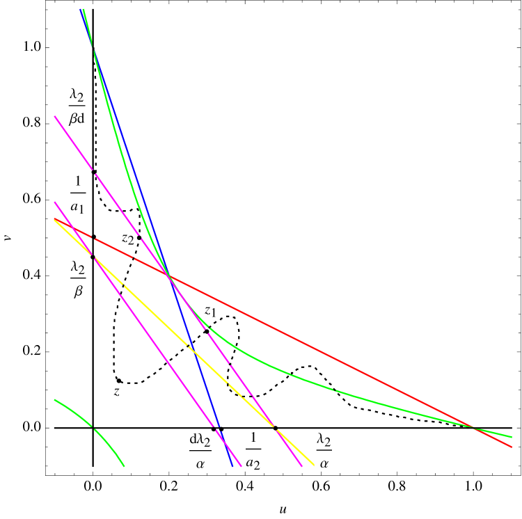
Let $\underaccent{\bar}{\mathcal{R}}=\{(u.v)\,|\,1-u-a_{1}\,v\geq 0,1-a_{2}\,u-v\geq 0,u\geq 0,v\geq 0\}$. First we construct an appropriate N-barrier consisting of three lines $\alpha\,u+d\,\beta\,v=\lambda_{2}$, $\alpha\,u+\beta\,v=\eta$ and $\alpha\,u+d\,\beta\,v=\lambda_{1}$, and chose $\lambda_{1}$, $\lambda_{2}$ and $\eta$ as large as possible such that $Q_{\lambda_{1}}\subset P_{\eta}\subset Q_{\lambda_{2}}\subset\underaccent{\bar}{\mathcal{R}}$, where $Q_{\lambda}=\{(u,v)\,|\,\alpha\,u+d\,\beta\,v\leq\lambda,u\geq 0,v\geq 0\}$ and $P_{\eta}=\{(u,v)\,|\,\alpha\,u+\beta\,v\leq\eta,u\geq 0,v\geq 0\}$. Then we show that $\lambda_{1}$ can be taken to equal the value on the right hand side of (2.3) and $q(x)\geq\lambda_{1}$ can be verified via the structure of the N-barrier.

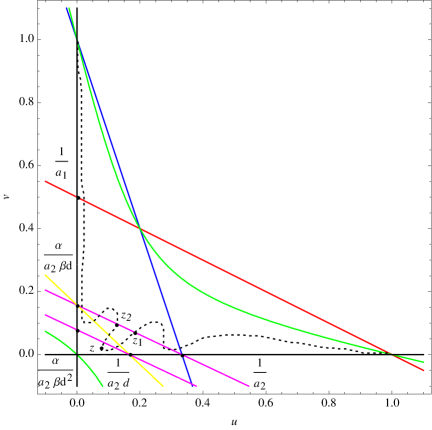
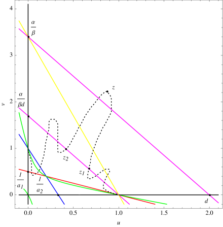
Now we illustrate how to construct the N-barrier in detail. For the case of $d\geq 1$ and $\beta\,a_{2}\,d\geq\alpha\,a_{1}$, the N-barrier is constructed in the following three steps (see Figure 2.2.1):

• The construction of the upper pink line: we draw on the $uv$-plane the upper pink line $\alpha\,u+d\,\beta\,v=\lambda_{2}$ which passes through $(\frac{1}{a_{2}},0)$. This gives $\lambda_{2}=\frac{\alpha}{a_{2}}$, and hence the upper pink line is represented by the equation $\alpha\,u+d\,\beta\,v=\frac{\alpha}{a_{2}}$. The $v$-coordinate of the $v$-intercept of $\alpha\,u+d\,\beta\,v=\frac{\alpha}{a_{2}}$ is $\frac{\alpha}{\beta\,a_{2}\,d}$, which is less than or equal to $\frac{1}{a_{1}}$ by the assumption $\beta\,a_{2}\,d\geq\alpha\,a_{1}$. This means that the $v$-coordinate of the $v$-intercept of $\alpha\,u+d\,\beta\,v=\frac{\alpha}{a_{2}}$ is below the $v$-coordinate of $v$-intercept of the $1-u-a_{1}\,v=0$.

• The construction of the yellow line: we let the the yellow line $\alpha\,u+\beta\,v=\eta$ start from $(0,\frac{\alpha}{\beta\,a_{2}\,d})$. This leads to $\eta=\frac{\alpha}{a_{2}\,d}$ and hence the yellow line is represented by the equation $\alpha\,u+\beta\,v=\frac{\alpha}{a_{2}\,d}$. The $u$-coordinate of the $u$-intercept of $\alpha\,u+\beta\,v=\frac{\alpha}{a_{2}\,d}$ is $\frac{1}{a_{2}\,d}$, which is less than or equal to $\frac{1}{a_{2}}$ by the assumption $d\geq 1$. This means that the $u$-coordinate of the $u$-intercept of $\alpha\,u+\beta\,v=\frac{\alpha}{a_{2}\,d}$ is less than or equal to the $u$-coordinate of $u$-intercept of $\alpha\,u+d\,\beta\,v=\frac{\alpha}{a_{2}}$.

• The construction of the lower pink line: we draw the lower pink line $\alpha\,u+d\,\beta\,v=\lambda_{1}$ passing through $(\frac{1}{a_{2}\,d},0)$. This gives $\lambda_{1}=\frac{\alpha}{a_{2}\,d}$.

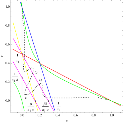
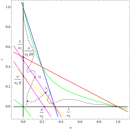
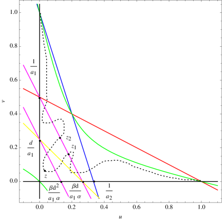
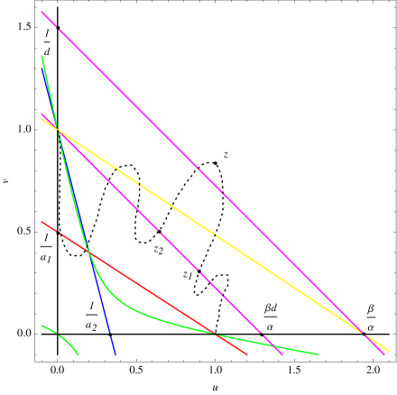
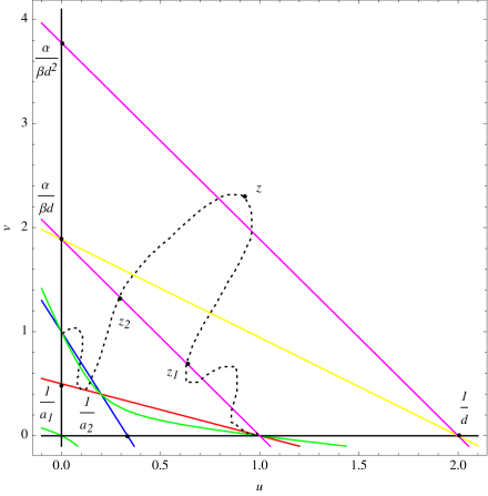
There are three other cases, each of which can be treated in a similar manner for the construction of the corresponding N-barrier (see Figures 2.2.1, 2.2.1, and 2.2.1). More precisely, we have the following four cases and for each case, we take different $\lambda_{1}$, $\lambda_{2}$ and $\eta$, and show that $q(x)$ has the lower bound $\lambda_{1}$ for $x\in\mathbb{R}$:

• If $d\geq 1$,

  • when $\beta\,a_{2}\,d\geq\alpha\,a_{1}$, we take $(\lambda_{1},\lambda_{2},\eta):=(\dfrac{\alpha}{a_{2}\,d},\dfrac{\alpha}{a_{2}},\dfrac{\alpha}{a_{2}\,d})$;

  • when $\beta\,a_{2}\,d<\alpha\,a_{1}$, we take $(\lambda_{1},\lambda_{2},\eta):=(\dfrac{\beta}{a_{1}},\dfrac{\beta\,d}{a_{1}},\dfrac{\beta}{a_{1}})$.

• If $d<1$,

  • when $\beta\,a_{2}\,d\geq\alpha\,a_{1}$, $(\lambda_{1},\lambda_{2},\eta):=(\dfrac{\alpha\,d}{a_{2}},\dfrac{\alpha}{a_{2}},\dfrac{\alpha}{a_{2}})$;

  • when $\beta\,a_{2}\,d<\alpha\,a_{1}$, $(\lambda_{1},\lambda_{2},\eta):=(\dfrac{\beta\,d^{2}}{a_{1}},\dfrac{\beta\,d}{a_{1}},\dfrac{\beta\,d}{a_{1}})$.

  We note that case $(i)$ corresponds to Figure 2.2.1, in which the N-barrier has been constructed in the above three steps. The other cases $(ii)$, $(iii)$, and $(iv)$ correspond to Figures 2.2.1, 2.2.1, and 2.2.1, respectively.

We first observe that the property $q(x)\geq\lambda_{1}$ in the four cases can be reduced to the following two cases:

• for $\beta\,a_{2}\,d\geq\alpha\,a_{1}$, $q(x)\geq\frac{\alpha}{a_{2}}\min[d,1/d]$ for all $x\in\mathbb{R}$;

• for $\beta\,a_{2}\,d<\alpha\,a_{1}$, $q(x)\geq\frac{\beta}{a_{1}}\min[1,d^{2}]$ for all $x\in\mathbb{R}$.

Combining the two cases above leads to $q(x)\geq\min[\frac{\alpha}{a_{2}\,d},\frac{\beta}{a_{1}}]\,\min[1,d^{2}]$ for all $x\in\mathbb{R}$, which is the desired result.

Now we show $q(x)\geq\lambda_{1}$ in $(i)\sim(iv)$. The two inequalities in (2.2) and (2.1) give

$$q^{\prime\prime}(x)+\theta\,p^{\prime}(x)+F(u(x),v(x))\leq 0.$$ (2.4)

For $d>1$, we first prove $(i)$ by contradiction. Suppose that, contrary to our claim, there exists $z\in\mathbb{R}$ such that $q(z)<\lambda_{1}$. Since $u,v\in C^{2}(\mathbb{R})$, by $(u,v)(-\infty)=(1,0)$ and $(u,v)(+\infty)=(0,1)$, we may assume $\min_{x\in\mathbb{R}}q(x)=q(z)$. We denote respectively by $z_{2}$ and $z_{1}$ the first points at which the solution $(u(x),v(x))$ intersects the line $\alpha\,u+d\,\beta\,v=\lambda_{2}$ in the $uv$-plane when $x$ moves from $z$ towards $\infty$ and $-\infty$ (as shown in Figure 2.2.1). For the case where $\theta\leq 0$, we integrate (2.4) with respect to $x$ from $z_{1}$ to $z$ and obtain

$$q^{\prime}(z)-q^{\prime}(z_{1})+\theta\,(p(z)-p(z_{1}))+\int_{z_{1}}^{z}F(u(x),v(x))\,dx\leq 0.$$ (2.5)

On the other hand we have:

• since $\min_{x\in\mathbb{R}}q(x)=q(z)$, $q^{\prime}(z)=\alpha\,u^{\prime}(z)+d\,\beta\,v^{\prime}(z)=0$;

• $q(z_{1})=\lambda_{2}$ follows from the fact that $z_{1}$ is on the line $\alpha\,u+d\,\beta\,v=\lambda_{2}$. Since $z_{1}$ is the first point for $q(x)$ taking the value $\lambda_{2}$ when $x$ moves from $z$ to $-\infty$, we conclude that $q(z_{1}+\delta)\leq\lambda_{2}$ for $z-z_{1}>\delta>0$ and $q^{\prime}(z_{1})\leq 0$;

• $p(z)<\eta$ since $z$ is below the line $\alpha\,u+\beta\,v=\eta$; $p(z_{1})>\eta$ since $z$ is above the line $\alpha\,u+\beta\,v=\eta$;

• it is readily seen that the quadratic curve $F(u,v)=0$ passes through the points $(0,0)$, $(1,0)$, $(0,1)$, and $(u^{\ast},v^{\ast})$ in the $uv$-plane. Let $A_{+}=\{(u,v)\,|\,F(u,v)\geq 0,u\geq 0,v\geq 0\}$. By Lemma 2.1 and the property that $F(u,v)<0$ for large $u$ and $v$, it follows that $A_{+}$ is the region bounded by a hyperbola, $u$-axis and $v$-axis. Moreover, $\{(u(x),v(x))\,|\,z_{1}\leq x\leq z\}$ $\subset\underaccent{\bar}{\mathcal{R}}$ $\subset A_{+}$. Therefore we have $\int_{z_{1}}^{z}F(u(x),v(x))\,dx>0$.

Summarizing the above arguments, we obtain

$$q^{\prime}(z)-q^{\prime}(z_{1})+\theta\,(p(z)-p(z_{1}))+\int_{z_{1}}^{z}F(u(x),v(x))\,dx>0,$$ (2.6)

which contradicts (2.5). Therefore when $\theta\leq 0$, $q(x)\geq\lambda_{1}$ for $x\in\mathbb{R}$. For the case where $\theta\geq 0$, integrating (2.4) with respect to $x$ from $z$ to $z_{2}$ yields

$$q^{\prime}(z_{2})-q^{\prime}(z)+\theta\,(p(z_{2})-p(z))+\int_{z}^{z_{2}}F(u(x),v(x))\,dx\leq 0.$$ (2.7)

In a similar manner, it can be shown that $q^{\prime}(z_{2})\geq 0$, $q^{\prime}(z)=0$, $p(z_{2})>\eta$, $p(z)<\eta$, and $\int_{z}^{z_{2}}F(u(x),v(x))\,dx>0$. These together contradict (2.7). Consequently, $(i)$ is proved for $d>1$. For $d=1$, we have $q=p$ and (2.4) becomes

$$p^{\prime\prime}(x)+\theta\,p^{\prime}(x)+F(u(x),v(x))\leq 0,\quad x\in\mathbb{R}.$$ (2.8)

Moreover, when $d=1$ we take $\lambda_{1}=\lambda_{2}=\eta=\frac{\alpha}{a_{2}}$, i.e. the three lines $\alpha\,u+d\,\beta\,v=\lambda_{1}$, $\alpha\,u+d\,\beta\,v=\lambda_{2}$, and $\alpha\,u+\beta\,v=\eta$ coincide. Analogously to the case of $d>1$, we assume that there exists $\hat{z}\in\mathbb{R}$ such that $p(\hat{z})<\lambda_{1}$ and $\min_{x\in\mathbb{R}}p(x)=p(\hat{z})$. Due to $\min_{x\in\mathbb{R}}p(x)=p(\hat{z})$, we have $p^{\prime}(\hat{z})=0$ and $p^{\prime\prime}(\hat{z})\geq 0$. Since $(u(\hat{z}),v(\hat{z}))$ is in the interior of $\underaccent{\bar}{\mathcal{R}}$, which is contained in the interior of $A_{+}$, we have $F(u(\hat{z}),v(\hat{z}))>0$. These together give $p^{\prime\prime}(\hat{z})+\theta\,p^{\prime}(\hat{z})+F(u(\hat{z}),v(\hat{z}))>0$, which contradicts (2.8). Thus, $p(x)\geq\lambda_{1}$ for all $x\in\mathbb{R}$ when $d=1$. As a result, the proof of $(i)$ is completed.

The proofs for cases $(ii)$, $(iii)$, and $(iv)$ are similar (see Figures 2.2.1, 2.2.1, and 2.2.1). This completes the proof of Proposition 2.2. ∎

       

Figure 2.1: Red line: $1-u-a_{1}\,v=0$; blue line: $1-a_{2}\,u-v=0$; green curve: $\alpha\,u\,(1-u-a_{1}\,v)+\beta\,k\,v\,(1-a_{2}\,u-v)=0$; magenta line (above): $\alpha\,u+d\,\beta\,v=\lambda_{2}$; magenta line (below): $\alpha\,u+d\,\beta\,v=\lambda_{1}$; yellow line: $\alpha\,u+\beta\,v=\eta$; dashed curve: $(u(x),v(x))$. 2.1 $a_{1}=2$, $a_{2}=3$, $\alpha=17$, $\beta=18$, and $d=2$ give $\lambda_{1}=\frac{17}{6}$, $\lambda_{2}=\frac{17}{3}$, and $\eta=\frac{17}{6}$. 2.1 $a_{1}=2$, $a_{2}=3$, $\alpha=17$, $\beta=5$, and $d=2$ give $\lambda_{1}=\frac{5}{2}$, $\lambda_{2}=5$, and $\eta=\frac{5}{2}$. 2.1 $a_{1}=2$, $a_{2}=3$, $\alpha=17$, $\beta=18$, and $d=\frac{2}{3}$ give $\lambda_{1}=\frac{34}{9}$, $\lambda_{2}=\frac{17}{3}$, and $\eta=\frac{17}{3}$. 2.1 $a_{1}=2$, $a_{2}=3$, $\alpha=17$, $\beta=18$, and $d=\frac{1}{2}$ give $\lambda_{1}=\frac{9}{4}$, $\lambda_{2}=\frac{9}{2}$, and $\eta=\frac{9}{2}$.

Proposition 2.3 (Upper bound for $q=q(x)$).

Assume that $a_{1}>1$, $a_{2}>1$, and that $(u(x),v(x))$ is $C^{2}$, nonnegative, and satisfies the following differential inequalities:

$$\begin{cases}\vspace{3mm}\hskip 5.69054ptu_{xx}+\theta\,u_{x}+\;\;u\,(1-u-a_{1}\,v)\geq 0,\quad x\in\mathbb{R},\\ \vspace{3mm}d\,v_{xx}+\theta\,v_{x}+k\,v\,(1-a_{2}\,u-v)\geq 0,\quad x\in\mathbb{R},\\ (u,v)(-\infty)=\text{\bf e}_{2},\quad(u,v)(+\infty)=\text{\bf e}_{3}.\end{cases}$$ (2.9)

Then for $x\in\mathbb{R}$, we have

$$q(x)\leq\max\bigg{[}\frac{\alpha}{d},\beta\bigg{]}\,\max[1,d^{2}].$$ (2.10)

Proof.

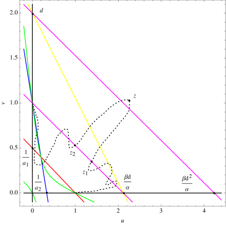
As in the proof of Proposition 2.2, there are also four cases and for each case, we can construct the N-barrier as shown in Figures 2.2.2, 2.2.2, 2.2.2, and 2.2.2 and prove that $q(x)\leq\lambda_{1}$ for $x\in\mathbb{R}$:

• If $d\geq 1$,

  • when $\beta\,d\geq\alpha$, we take $(\lambda_{1},\lambda_{2},\eta):=(\beta\,d^{2},\beta\,d,\beta\,d)$;

  • when $\beta\,d<\alpha$, $(\lambda_{1},\lambda_{2},\eta):=(\alpha\,d,\alpha,\alpha)$.

• If $d<1$,

  • when $\beta\,d\geq\alpha$, $(\lambda_{1},\lambda_{2},\eta):=(\beta,\beta\,d,\beta)$;

  • when $\beta\,d<\alpha$, $(\lambda_{1},\lambda_{2},\eta):=(\dfrac{\alpha}{d},\alpha,\dfrac{\alpha}{d})$.

We note that cases $(i)$, $(ii)$, $(iii)$, and $(iv)$ corresponds to Figures 2.2.2, 2.2.2, 2.2.2, and 2.2.2, respectively. Combining the four cases above, it follows that

• for $\beta\,d\geq\alpha$, $q(x)\leq\beta\max(1,d^{2})$ for all $x\in\mathbb{R}$;

• for $\beta\,d<\alpha$, $q(x)\leq\alpha\max(d,1/d)$ for all $x\in\mathbb{R}$,

which implies $q(x)\leq\max[\frac{\alpha}{d},\beta]\,\max[1,d^{2}]$ for all $x\in\mathbb{R}$. The rest part of the proof is similar to that of Proposition 2.2 and is hence omitted.

       

Figure 2.2: Red line: $1-u-a_{1}\,v=0$; blue line: $1-a_{2}\,u-v=0$; green curve: $\alpha\,u\,(1-u-a_{1}\,v)+\beta\,k\,v\,(1-a_{2}\,u-v)=0$; magenta line (below): $\alpha\,u+d\,\beta\,v=\lambda_{2}$; magenta line (above): $\alpha\,u+d\,\beta\,v=\lambda_{1}$; yellow line: $\alpha\,u+\beta\,v=\eta$; dashed curve: $(u(x),v(x))$. 2.2 $a_{1}=2$, $a_{2}=3$, $\alpha=17$, $\beta=18$, and $d=2$ give $\lambda_{1}=72$, $\lambda_{2}=36$, and $\eta=36$. 2.2 $a_{1}=2$, $a_{2}=3$, $\alpha=17$, $\beta=5$, and $d=2$ give $\lambda_{1}=34$, $\lambda_{2}=17$, and $\eta=17$. 2.2 $a_{1}=2$, $a_{2}=3$, $\alpha=17$, $\beta=33$, and $d=\frac{2}{3}$ give $\lambda_{1}=33$, $\lambda_{2}=22$, and $\eta=33$. 2.2 $a_{1}=2$, $a_{2}=3$, $\alpha=17$, $\beta=18$, and $d=\frac{1}{2}$ give $\lambda_{1}=34$, $\lambda_{2}=17$, and $\eta=34$.

∎

3 General maximum principle

In this section, we prove Theorem 1.2, which generalizes the maximum principle in Theorem 1.1 to elliptic systems with a wider class of nonlinear terms. Recall that $\bar{\mathcal{R}}=\big{\{}(u,v)\;\big{|}\;\frac{u}{\bar{u}}+\frac{v}{\bar{v}}\geq 1,\;u,v\geq 0\big{\}}$ and $\underaccent{\bar}{\mathcal{R}}=\big{\{}(u,v)\;\big{|}\;\frac{u}{\underaccent{\bar}{u}}+\frac{v}{\underaccent{\bar}{v}}\leq 1,\;u,v\geq 0\big{\}}$.

As in Section 2, adding the two equations in (1.10) leads to an equation involving $p(x)=\alpha\,u(x)+\beta\,v(x)$ and $q(x)=d_{1}\,\alpha\,u(x)+d_{2}\,\beta\,v(x)$, i.e.

$$0 =\alpha\,\big{(}d_{1}\,u_{xx}+\theta\,u_{x}+u^{m}\,f(u,v)\big{)}+\beta\,\big{(}d_{2}\,v_{xx}+\theta\,v_{x}+v^{n}\,g(u,v)\big{)}$$

$$=q^{\prime\prime}(x)+\theta\,p^{\prime}(x)+\alpha\,u^{m}\,f(u,v)+\beta\,v^{n}\,g(u,v)$$

$$=q^{\prime\prime}(x)+\theta\,p^{\prime}(x)+F(u,v),$$ (3.1)

where $\alpha$, $\beta>0$ are arbitrary constants and $F(u,v)=\alpha\,u^{m}\,f(u,v)+\beta\,v^{n}\,g(u,v)$. By assumption $\mathbf{[A]}$, it readily follows that $F(u,v)\geq 0$ on $\underaccent{\bar}{\mathcal{R}}$ and $F(u,v)\leq 0$ on $\bar{\mathcal{R}}$. In Theorem 1.2, when $\text{\bf e}_{-}=(0,0)$ or $\text{\bf e}_{+}=(0,0)$, the lower bound estimate no longer holds but the upper bound estimate is still valid. In the following, we state a theorem, which is slightly more general than Theorem 1.2, to include the upper bound estimate when $\text{\bf e}_{-}=(0,0)$ or $\text{\bf e}_{+}=(0,0)$.

Theorem 3.1.

Assume that $\mathbf{[A]}$ holds. If $a>0$, $b>0$, and $(u(x),v(x))$ is a nonnegative solution to (1.10), then

$$\underaccent{\bar}{\lambda}\leq a\,u(x)+b\,v(x)\leq\bar{\lambda},\quad x\in\mathbb{R},$$ (3.2)

where

$$\bar{\lambda}=\max\big{(}a\,\bar{u},b\,\bar{v}\big{)}\,\frac{\max(d_{1},d_{2})}{\min(d_{1},d_{2})}$$ (3.3)

and

$$\underaccent{\bar}{\lambda}=\min\big{(}a\,\underaccent{\bar}{u},b\,\underaccent{\bar}{v}\big{)}\,\frac{\displaystyle\min(d_{1},d_{2})}{\displaystyle\max(d_{1},d_{2})}\,\chi.$$ (3.4)

with $\chi$ defined by

$$\chi=\begin{cases}\vspace{3mm}0,\quad\text{if}\quad\text{\bf e}_{+}=(0,0)\quad\text{or}\quad\text{\bf e}_{-}=(0,0),\\ 1,\quad\text{otherwise}.\end{cases}$$ (3.5)

Proof.

Let $\alpha=a/d_{1}$ and $\beta=b/d_{2}$ in (3). Then $q(x)=au(x)+bv(x)$ in (3). We employ the N-barrier method developed in Section 2 to show (3.2), which implies (1.11).

First, we assume $\text{\bf e}_{+}\neq(0,0)$ and $\text{\bf e}_{-}\neq(0,0)$. To construct an appropriate N-barrier for the lower bound estimate, we consider $Q_{\lambda}=\{(u,v)\,|\,d_{1}\,\alpha\,u+d_{2}\,\beta\,v\leq\lambda,u\geq 0,v\geq 0\}$ and $P_{\eta}=\{(u,v)\,|\,\alpha\,u+\beta\,v\leq\eta,u\geq 0,v\geq 0\}$, and chose $\lambda_{1}$, $\lambda_{2}$ and $\eta$ as large as possible such that $Q_{\lambda_{1}}\subset P_{\eta}\subset Q_{\lambda_{2}}\subset\underaccent{\bar}{\mathcal{R}}$. By direct computation, $\lambda_{1}$, $\lambda_{2}$ and $\eta$ can be determined by

$$\lambda_{2} = \min\,(d_{1}\alpha\,\underaccent{\bar}{u},d_{2}\alpha\,\underaccent{\bar}{v})\,=\,\min\big{(}a\underaccent{\bar}{u},b\underaccent{\bar}{v}\big{)},$$ (3.6)

$$\eta = \min\,(\frac{1}{d_{1}},\frac{1}{d_{2}})\,\lambda_{2},$$ (3.7)

$$\lambda_{1} = \min\,(d_{1},d_{2})\,\eta=\min\,(\frac{d_{1}}{d_{2}},\frac{d_{2}}{d_{1}})\,\lambda_{2}.$$ (3.8)

Since $F(u,v)\geq 0$ on $\underaccent{\bar}{\mathcal{R}}$, we can employ (3) and follow the arguments in Section 2 to obtain the lower bound estimate $q(x)\geq\lambda_{1}=\underaccent{\bar}{\lambda}$.

When the boundary conditions $\text{\bf e}_{+}=(0,0)$ or $\text{\bf e}_{-}=(0,0)$, the argument in Section 2 can not be applied and only a trivial lower bound $a\,u(x)+b\,v(x)\geq 0$ can be given.

The proof for the upper bound of $a\,u+b\,v$ is similar. ∎

4 More delicate lower bound: tangent lines to quadratic curves

In this section we provide an alternative approach to determine the line $\alpha\,u+d\,\beta\,v=\lambda_{2}$ in the proof of Proposition 2.2 so that a bigger $\lambda_{2}$ can be chosen and a stronger lower bound for $q(x)$ can be given. To this end, we determine $\lambda_{2}$ by solving

$$\alpha\,u+d\,\beta\,v=\lambda_{2},$$ (4.1a)

$$F(u,v)=0,$$ (4.1b)

$$\frac{F_{u}(u,v)}{\alpha}=\frac{F_{v}(u,v)}{d\,\beta},$$ (4.1c)

where $F_{u}(u,v)=\frac{\partial F}{\partial u}(u,v)$ and $F_{v}(u,v)=\frac{\partial F}{\partial v}(u,v)$. In (4.1), $\alpha\,u+d\,\beta\,v=\lambda_{2}$ is the tangent line to the quadratic curve $F(u,v)=0$ and the line $\alpha\,u+d\,\beta\,v=\lambda_{2}$ is perpendicular to the vector $<F_{u}(u,v),F_{v}(u,v)>$. The solution $(u,v,\lambda_{2})$ of (4.1) determines the point of tangency of the line $\alpha\,u+d\,\beta\,v=\lambda_{2}$ and the quadratic curve $F(u,v)=0$.

Equation (4.1) can be solved with the aid of Mathematica. It is easy to see that the first and third equations in (4.1) are linear, while the second one is quadratic. To solve (4.1), we begin by solving the first and third equations to obtain $(u,v)=(u(\lambda_{2}),v(\lambda_{2}))$ as

, namely

$$u=\frac{-d\lambda_{2}\left(\alpha a_{1}+a_{2}\beta k\right)+\alpha\beta d(d-k)+2\alpha k\lambda_{2}}{2\alpha\left(-d\left(\alpha a_{1}+a_{2}\beta k\right)+\beta d^{2}+\alpha k\right)},$$ (4.2a)

$$v=\frac{\alpha a_{1}\lambda_{2}+\beta\left(a_{2}k\lambda_{2}+\alpha d-2d\lambda_{2}-\alpha k\right)}{2\beta\left(\alpha a_{1}d+a_{2}\beta dk-\beta d^{2}-\alpha k\right)}.$$ (4.2b)

Substituting (4.2) into the second equation in (4.1) yields the following quadratic equation for $\lambda_{2}$:

$$\mu_{2}\,\lambda_{2}^{2}+\mu_{1}\,\lambda_{2}+\mu_{0}=0,$$ (4.3)

where

$$\mu_{2}=\frac{\left(\alpha a_{1}+a_{2}\beta k\right)^{2}-4\alpha\beta k}{4\alpha\beta\left(-d\left(\alpha a_{1}+a_{2}\beta k\right)+\beta d^{2}+\alpha k\right)},$$ (4.4a)

$$\mu_{1}=\frac{-2\alpha\beta\left((d+k)\left(\alpha a_{1}+a_{2}\beta k\right)-2k(\alpha+\beta d)\right)}{4\alpha\beta\left(-d\left(\alpha a_{1}+a_{2}\beta k\right)+\beta d^{2}+\alpha k\right)},$$ (4.4b)

$$\mu_{0}=\frac{\alpha\beta(d-k)^{2}}{4\left(-d\left(\alpha a_{1}+a_{2}\beta k\right)+\beta d^{2}+\alpha k\right)}.$$ (4.4c)

It follows from (4.3) that

$$\lambda_{2}=\frac{-\mu_{1}\pm\sqrt{\mu_{1}^{2}-4\mu_{0}\mu_{2}}}{2\mu_{2}}.$$ (4.5)

Using (4.4), the discriminant $\mathcal{D}$ of (4.3) is given by

$$\mathcal{D}=\mu_{1}^{2}-4\mu_{2}\mu_{0}=\frac{k\left(-a_{1}\alpha-a_{2}\beta k+\alpha+\beta k\right)}{-d\left(\alpha a_{1}+a_{2}\beta k\right)+\beta d^{2}+\alpha k}.$$ (4.6)

To apply the approach proposed here, it is necessary that $\mathcal{D}\geq 0$. In fact, $\mathcal{D}\neq 0$ since $k\left(-a_{1}\alpha-a_{2}\beta k+\alpha+\beta k\right)=k(\alpha(1-a_{1})+k\beta(1-a_{2}))<0$. Moreover, it can be shown that $\mathcal{D}>0$ if and only if

$$\frac{\alpha a_{1}+a_{2}\beta k-\sqrt{\left(\alpha a_{1}+a_{2}\beta k\right){}^{2}-4\alpha\beta k}}{2\beta}<d<\frac{\alpha a_{1}+a_{2}\beta k+\sqrt{\left(\alpha a_{1}+a_{2}\beta k\right){}^{2}-4\alpha\beta k}}{2\beta}.$$ (4.7)

Under the condition (4.7), $\mu_{0}<0$, $\mu_{1}>0$, and $\mu_{2}<0$ and hence the two roots $\lambda_{2}$ given by (4.5) are both positive. However, when

$$\lambda_{2}=\frac{-\mu_{1}+\sqrt{\mu_{1}^{2}-4\mu_{0}\mu_{2}}}{2\mu_{2}},$$ (4.8)

it turns out that one of $u,v$ given by (4.2) is negative. We remark that this fact can also be easily seen from a property of the hyperbola $F(u,v)=0$. That is, for a given slope, there exist two tangent lines to the hyperbola $F(u,v)=0$: one has the intersection point in the first quadrant, while the other has the intersection point in the second or fourth quadrant. Therefore, we have

$$\lambda_{2}=\frac{-\mu_{1}-\sqrt{\mu_{1}^{2}-4\mu_{0}\mu_{2}}}{2\mu_{2}}$$ (4.9)

and the intersection point $(u,v)$ can be expressed in terms of $\lambda_{2}$ using (4.2). Now we are in a position to prove:

Proposition 4.1 (Stronger lower bound for $q=q(x)$).

Assume that $a_{1}>1$, $a_{2}>1$ and the condition (4.7) holds. Let $\lambda_{2}$ be given by (4.9) and let $(u(x),v(x))$ be a pair of nonnegative $C^{2}$ functions satisfying the differential inequalities (2.2). Then we have

• when $d\geq 1$, $q(x)\geq\,\dfrac{\lambda_{2}}{d}$ for all $x\in\mathbb{R}$;

• when $d<1$, $q(x)\geq\,\lambda_{2}\,d$ for all $x\in\mathbb{R}$.

Consequently, for $d>0$ we have $q(x)\geq\lambda_{2}\,\min[d,1/d]$ for all $x\in\mathbb{R}$.

Proof.

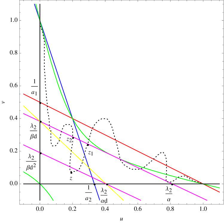
The proof is similar to that of Proposition 2.2 (see Figure 4.1 and Figure 4.2). Here we only explain how to determine $(\lambda_{1},\eta)$ (see Figure 4.2). When $d<1$, we choose $(\lambda_{1},\eta)=(\lambda_{2}\,d,\lambda_{2})$ via the following procedure. The line $\alpha\,u+d\,\beta\,v=\lambda_{2}$ intersects the $u$-axis and $v$-axis at $(\frac{\lambda_{2}}{\alpha},0)$ and $(0,\frac{\lambda_{2}}{\beta d})$, respectively. Since $d<1$, the line $\alpha\,u+\beta\,v=\eta$ passes through the point $(\frac{\lambda_{2}}{\alpha},0)$, and $\eta$ is determined by $\eta=\alpha\,u+\beta\,v\Big{|}_{(u,v)=\left(\frac{\lambda_{2}}{\alpha},0\right)}=\lambda_{2}$. The line $\alpha\,u+\beta\,v=\eta$ intersects the $v$-axis at $(0,\frac{\lambda_{2}}{\beta})$, so $\lambda_{1}$ is given by $\lambda_{1}=\alpha\,u+d\,\beta\,v\Big{|}_{(u,v)=\left(0,\frac{\lambda_{2}}{\beta}\right)}=\lambda_{2}\,d$. For the case $d\geq 1$, $\lambda_{1}$ and $\eta$ can be determined in a similar manner as $(\lambda_{1},\eta)=(\frac{\lambda_{2}}{d},\frac{\lambda_{2}}{d})$. (Refer to Figure 4.1.)

∎

Combining Propositions 2.3 and 4.1, we obtain

Corollary 4.2 (Maximum principle for $q(x)$).

Assume that $a_{1}>1$, $a_{2}>1$ and the condition (4.7) holds. Let $\lambda_{2}$ be given by (4.9) and let $(u(x),v(x))$ be a nonnegative solution to the following differential equations and asymptotic conditions

$$\begin{cases}\vspace{3mm}u_{xx}+\theta\,u_{x}+u\,(1-u-a_{1}\,v)=0,\quad x\in\mathbb{R},\\ \vspace{3mm}v_{xx}+\theta\,v_{x}+v\,(1-a_{2}\,u-v)=0,\quad x\in\mathbb{R},\\ (u,v)(-\infty)=(1,0),\quad(u,v)(+\infty)=(0,1).\end{cases}$$ (4.10)

Then for $x\in\mathbb{R}$, we have

$$\frac{\lambda_{2}}{d}\,\min[1,d^{2}]\leq q(x)\leq\max\Big{[}\frac{\alpha}{d},\beta\Big{]}\max[1,d^{2}].$$ (4.11)

Compared with Theorem 1.1, Corollary 4.2 asserts that when (4.7) holds, a stronger lower bound for $q(x)$ can be given in terms of $\lambda_{2}$, which is defined by (4.9). In particular, when $\alpha=\beta=d=k=1$, we obtain Theorem 1.3.

To illustrate Proposition 4.1, we give an example. When $a_{1}=2$, $a_{2}=3$, $\alpha=17$, $\beta=18$, $d=2$, and $k=1$, (4.1) can be solved to give

$$(u,v,\lambda_{2})=\bigg{(}\frac{3\left(2349\pm 71\sqrt{4611}\right)}{47270},\frac{17\left(1131\pm 4\sqrt{4611}\right)}{141810},\frac{153\left(79\pm\sqrt{4611}\right)}{1630}\bigg{)},$$ (4.12)

which is approximately $(u,v,\lambda_{2})=(-0.157,0.103,1.0415)$ or $(0.455,0.168,13.789)$. We choose $(u,v,\lambda_{2})=\left(\frac{3\left(2349+71\sqrt{4611}\right)}{47270},\frac{17\left(1131+4\sqrt{4611}\right)}{141810},\frac{153\left(79+\sqrt{4611}\right)}{1630}\right)\approx(0.455,0.168,13.789)$, and determine

$$\lambda_{1}=\eta=\frac{\lambda_{2}}{d}$$ (4.13)

by employing Proposition 4.1. Then we are led to Figure 4.1. Applying Proposition 4.1 again, it follows that $q(x)\geq\lambda_{1}\approx 6.895$ for all $x\in\mathbb{R}$ (see Figure 4.1). This lower bound is much bigger compared with the one given previously in Section 2, where the lower bound for $q(x)$ is $\frac{17}{6}\approx 2.833$ (see Figure 2.2.1).

Figure 4.1: Red line: $1-u-a_{1}\,v=0$; blue line: $1-a_{2}\,u-v=0$; green curve: $\alpha\,u\,(1-u-a_{1}\,v)+\beta\,k\,v\,(1-a_{2}\,u-v)=0$; magenta line (above): $\alpha\,u+d\,\beta\,v=\lambda_{2}$; magenta line (below): $\alpha\,u+d\,\beta\,v=\lambda_{1}$; yellow line: $\alpha\,u+\beta\,v=\eta$; dashed curve: $(u(x),v(x))$. $a_{1}=2$, $a_{2}=3$, $\alpha=17$, $\beta=18$, $d=2$, $k=1$, and $\lambda_{2}=\frac{153\left(79+\sqrt{4611}\right)}{1630}\approx 13.789$ give $\lambda_{1}=\eta=\frac{153\left(79+\sqrt{4611}\right)}{3260}\approx 6.895$ according to (4.13) .

Figure 4.2: Red line: $1-u-a_{1}\,v=0$; blue line: $1-a_{2}\,u-v=0$; green curve: $\alpha\,u\,(1-u-a_{1}\,v)+\beta\,k\,v\,(1-a_{2}\,u-v)=0$; magenta line (upper): $\alpha\,u+d\,\beta\,v=\lambda_{2}$; magenta line (lower): $\alpha\,u+d\,\beta\,v=\lambda_{1}$; yellow line: $\alpha\,u+\beta\,v=\eta$; dashed curve: $(u(x),v(x))$. $a_{1}=2$, $a_{2}=3$, $\alpha=17$, $\beta=18$, $d=\frac{2}{3}$, $k=1$, and $\lambda_{2}=\frac{51\left(133+\sqrt{16059}\right)}{1630}\approx 8.126$ give $\lambda_{1}=\lambda_{2}\,d=\frac{17}{815}\left(133+\sqrt{16059}\right)\approx 5.418$ and $\eta=\lambda_{2}=\frac{51\left(133+\sqrt{16059}\right)}{1630}\approx 8.126$ .

5 Application to the nonexistence of three species travelling waves: proof of Theorem 1.4

In this section, we prove Theorem 1.4 by contradiction.

Proof of Theorem 1.4.

Suppose to the contrary that there exists a solution $(u(x),v(x),w(x))$ to (1.13),(1.14). Due to the fact that $w(x)>0$ for $x\in\mathbb{R}$ and $w(\pm\infty)=0$, we can find $x_{0}\in\mathbb{R}$ such that $\max_{x\in\mathbb{R}}w(x)=w(x_{0})>0$, $w^{\prime\prime}(x_{0})\leq 0$, and $w^{\prime}(x_{0})=0$. Since $w(x)$ satisfies $d_{3}\,w_{xx}+\theta\,w_{x}+w(\sigma_{3}-c_{31}\,u-c_{32}\,v-c_{33}\,w)=0$, we obtain

$$\sigma_{3}-c_{31}\,u(x_{0})-c_{32}\,v(x_{0})-c_{33}\,w(x_{0})\geq 0,$$ (5.1)

which gives

$$w(x)\leq w(x_{0})\leq\frac{1}{c_{33}}\big{(}\sigma_{3}-c_{31}\,u(x_{0})-c_{32}\,v(x_{0})\big{)}<\frac{\sigma_{3}}{c_{33}},\;x\in\mathbb{R}.$$ (5.2)

As a consequence, we have

$$\begin{cases}\vspace{3mm}d_{1}\,u_{xx}+\theta\,u_{x}+u(\sigma_{1}-c_{13}\,\sigma_{3}\,c_{33}^{-1}-c_{11}\,u-c_{12}\,v)\leq 0,\quad x\in\mathbb{R},\\ d_{2}\,v_{xx}\hskip 2.27621pt+\theta\,v_{x}+v(\sigma_{2}-c_{23}\,\sigma_{3}\,c_{33}^{-1}-c_{21}\,u-c_{22}\,v)\leq 0,\quad x\in\mathbb{R}.\end{cases}$$ (5.3)

Because of $\mathbf{[H1]}$ and $\mathbf{[H2]}$, we can apply Proposition 6.1 from the Appendix to (5.3). Indeed, $\mathbf{[H1]}$ assures the positivity of $\sigma_{1}-c_{13}\,\sigma_{3}\,c_{33}^{-1}$ and $\sigma_{2}-c_{23}\,\sigma_{3}\,c_{33}^{-1}$, while the bistability condition $\mathbf{[BiS]}$ (see Appendix) for the nonlinearity in (5.3) follows from $\mathbf{[H2]}$. Consequently, we obtain a lower bound of $c_{31}\,u(x)+c_{32}\,v(x)$, i.e.

$$c_{31}\,u(x)+c_{32}\,v(x)\geq c_{33}^{-1}\,\min\bigg{[}\frac{\displaystyle c_{31}\,\phi_{2}}{\displaystyle c_{21}\,d_{2}},\frac{\displaystyle c_{32}\,\phi_{1}}{\displaystyle c_{12}\,d_{1}}\bigg{]}\,\min\big{[}d_{1}^{2},d_{2}^{2}\big{]},\;x\in\mathbb{R}.$$ (5.4)

The condition $\mathbf{[H3]}$ then yields

$$c_{31}\,u(x)+c_{32}\,v(x)\geq\sigma_{3},\;x\in\mathbb{R},$$ (5.5)

which contradicts (5.1). This completes the proof.

∎

6 Appendix

After suitable scaling, system (1.4) is equivalent to (1.5). Theorem 1.1 establishes lower-upper bound estimates for (1.4). In this section, we state corresponding results for (1.5). Throughout this section, we shall always assume the bistable condition:

• $\frac{\displaystyle\sigma_{1}}{\displaystyle c_{11}}>\frac{\displaystyle\sigma_{2}}{\displaystyle c_{21}}$, $\frac{\displaystyle\sigma_{2}}{\displaystyle c_{22}}>\frac{\displaystyle\sigma_{1}}{\displaystyle c_{12}}$,

which correponds to the condition $a_{1}>1$ and $a_{2}>1$ used in previous sections. Let $p(x)=\alpha\,u+\beta\,v$ and $q(x)=d_{1}\,\alpha\,u+d_{2}\,\beta\,v$. Then, from (1.5), it follows that $p(x)$ and $q(x)$ satisfy

$$\alpha\,\big{(}d_{1}\,u_{xx}+\theta\,u_{x}+u\,(\sigma_{1}-c_{11}\,u-c_{12}\,v)\big{)}+\beta\,\big{(}d_{2}\,v_{xx}+\theta\,v_{x}+v\,(\sigma_{2}-c_{21}\,u-c_{22}\,v)\big{)}$$

$$=q^{\prime\prime}(x)+\theta\,p^{\prime}(x)+\alpha\,u\,(\sigma_{1}-c_{11}\,u-c_{12}\,v)+\beta\,v\,(\sigma_{2}-c_{21}\,u-c_{22}\,v).$$

We can now apply the approach proposed in Section 2 to obtain lower and upper bounds for $q(x)$ in Proposition 6.1 and Proposition 6.2, respectively.

Proposition 6.1 (Lower bound for $q=q(x)$).

Suppose that $(u(x),v(x))$ is $C^{2}$ and nonnegative, and satisfies the differential inequalities

$$\begin{cases}\vspace{3mm}d_{1}\,u_{xx}+\theta\,u_{x}+u\,(\sigma_{1}-c_{11}\,u-c_{12}\,v)\leq 0,\quad x\in\mathbb{R},\\ \vspace{3mm}d_{2}\,v_{xx}\hskip 2.27621pt+\theta\,v_{x}+v\,(\sigma_{2}-c_{21}\,u-c_{22}\,v)\leq 0,\quad x\in\mathbb{R},\\ (u,v)(-\infty)=\big{(}\frac{\displaystyle\sigma_{1}}{\displaystyle c_{11}},0\big{)},\quad(u,v)(+\infty)=\big{(}0,\frac{\displaystyle\sigma_{2}}{\displaystyle c_{22}}\big{)}.\end{cases}$$ (6.2)

Then for $x\in\mathbb{R}$, we have

$$q(x)\geq\min\bigg{[}\frac{\alpha\,\sigma_{2}}{c_{21}\,d_{2}},\frac{\beta\,\sigma_{1}}{c_{12}\,d_{1}}\bigg{]}\,\min\big{[}d_{1}^{2},d_{2}^{2}\big{]}.$$ (6.3)

Proposition 6.2 (Upper bound for $q=q(x)$).

Suppose that $(u(x),v(x))$ is $C^{2}$ and nonnegative, and satisfies the following differential inequalities and asymptotic conditions

$$\begin{cases}\vspace{3mm}d_{1}\,u_{xx}+\theta\,u_{x}+u\,(\sigma_{1}-c_{11}\,u-c_{12}\,v)\geq 0,\quad x\in\mathbb{R},\\ \vspace{3mm}d_{2}\,v_{xx}\hskip 2.27621pt+\theta\,v_{x}+v\,(\sigma_{2}-c_{21}\,u-c_{22}\,v)\geq 0,\quad x\in\mathbb{R},\\ (u,v)(-\infty)=\big{(}\frac{\displaystyle\sigma_{1}}{\displaystyle c_{11}},0\big{)},\quad(u,v)(+\infty)=\big{(}0,\frac{\displaystyle\sigma_{2}}{\displaystyle c_{22}}\big{)}.\end{cases}$$ (6.4)

Then for $x\in\mathbb{R}$, we have

$$q(x)\leq\max\bigg{[}\frac{\alpha\,\sigma_{1}}{c_{11}\,d_{2}},\frac{\beta\,\sigma_{2}}{c_{22}\,d_{1}}\bigg{]}\,\max\big{[}d_{1}^{2},d_{2}^{2}\big{]}.$$ (6.5)

Theorem 6.3 (Maximum principle for $q(x)$).

Suppose that $(u(x),v(x))$ is a nonnegative solution to the differential equations

$$\begin{cases}\vspace{3mm}d_{1}\,u_{xx}+\theta\,u_{x}+u\,(\sigma_{1}-c_{11}\,u-c_{12}\,v)=0,\quad x\in\mathbb{R},\\ \vspace{3mm}d_{2}\,v_{xx}\hskip 2.27621pt+\theta\,v_{x}+v\,(\sigma_{2}-c_{21}\,u-c_{22}\,v)=0,\quad x\in\mathbb{R},\\ (u,v)(-\infty)=\big{(}\frac{\displaystyle\sigma_{1}}{\displaystyle c_{11}},0\big{)},\quad(u,v)(+\infty)=\big{(}0,\frac{\displaystyle\sigma_{2}}{\displaystyle c_{22}}\big{)}.\end{cases}$$ (6.6)

Then for $x\in\mathbb{R}$, we have

$$\min\bigg{[}\frac{\alpha\,\sigma_{2}}{c_{21}\,d_{2}},\frac{\beta\,\sigma_{1}}{c_{12}\,d_{1}}\bigg{]}\,\min\big{[}d_{1}^{2},d_{2}^{2}\big{]}\leq q(x)\leq\max\bigg{[}\frac{\alpha\,\sigma_{1}}{c_{11}\,d_{2}},\frac{\beta\,\sigma_{2}}{c_{22}\,d_{1}}\bigg{]}\,\max\big{[}d_{1}^{2},d_{2}^{2}\big{]}.$$ (6.7)

Proof.

Combining Proposition 6.1 and Proposition 6.2, Theorem 6.3 is established. ∎

We note in particular that, when $\alpha=d_{1}^{-1}$ and $\beta=d_{2}^{-1}$, (6.7) becomes

$$\min\bigg{[}\frac{\sigma_{2}}{c_{21}},\frac{\sigma_{1}}{c_{12}}\bigg{]}\,\min\bigg{[}\frac{d_{1}}{d_{2}},\frac{d_{2}}{d_{1}}\bigg{]}\leq u(x)+v(x)\leq\max\bigg{[}\frac{\sigma_{1}}{c_{11}},\frac{\sigma_{2}}{c_{22}}\bigg{]}\,\max\bigg{[}\frac{d_{1}}{d_{2}},\frac{d_{2}}{d_{1}}\bigg{]}.$$ (6.8)

The above result can be generalised by letting $\alpha=d_{1}^{-1}\,r_{1}$ and $\beta=d_{2}^{-1}\,r_{2}$. Equation (6.7) then leads to

$$\min\bigg{[}\dfrac{r_{1}\sigma_{2}}{c_{21}},\dfrac{r_{2}\sigma_{1}}{c_{12}}\bigg{]}\min\bigg{[}\dfrac{d_{1}}{d_{2}},\dfrac{d_{2}}{d_{1}}\bigg{]} \leq r_{1}u(x)+r_{2}v(x)$$ (6.9)

$$\leq \max\bigg{[}\dfrac{r_{1}\sigma_{1}}{c_{11}},\dfrac{r_{2}\sigma_{2}}{c_{22}}\bigg{]}\max\bigg{[}\dfrac{d_{1}}{d_{2}},\dfrac{d_{2}}{d_{1}}\bigg{]},$$

where $r_{1},r_{2}>0$ are arbitrary constants.

Acknowledgments. The authors wish to express sincere gratitude to Dr. Tom Mollee for his careful reading of the manuscript and valuable suggestions and comments to improve the readability and accuracy of the paper. CC Chen are grateful for the support by the grant 102-2115-M-002-011-MY3 of Ministry of Science and Technology, Taiwan. The research of L.-C. Hung is partly supported by the grant 104EFA0101550 of Ministry of Science and Technology, Taiwan.

References

• [1] C.-C. Chen and L.-C. Hung, Nonexistence of traveling wave solutions, exact and semi-exact traveling wave solutions for diffusive lotka-volterra systems of three competing species, Communications on Pure and Applied Analysis, To appear.
• [2] C.-C. Chen, L.-C. Hung, M. Mimura, and D. Ueyama, Exact travelling wave solutions of three-species competition-diffusion systems, Discrete Contin. Dyn. Syst. Ser. B, 17 (2012), pp. 2653–2669.
• [3] P. de Mottoni, Qualitative analysis for some quasilinear parabolic systems, Institute of Math., Polish Academy Sci., zam, 11 (1979), p. 190.
• [4] N. Fei and J. Carr, Existence of travelling waves with their minimal speed for a diffusing Lotka-Volterra system, Nonlinear Anal. Real World Appl., 4 (2003), pp. 503–524.
• [5] L.-C. Hung, Exact traveling wave solutions for diffusive Lotka-Volterra systems of two competing species, Jpn. J. Ind. Appl. Math., 29 (2012), pp. 237–251.
• [6] Y. Kan-on, Parameter dependence of propagation speed of travelling waves for competition-diffusion equations, SIAM J. Math. Anal., 26 (1995), pp. 340–363.
• [7]  , Fisher wave fronts for the Lotka-Volterra competition model with diffusion, Nonlinear Anal., 28 (1997), pp. 145–164.
• [8] A. W. Leung, X. Hou, and W. Feng, Traveling wave solutions for Lotka-Volterra system re-visited, Discrete Contin. Dyn. Syst. Ser. B, 15 (2011), pp. 171–196.
• [9] A. W. Leung, X. Hou, and Y. Li, Exclusive traveling waves for competitive reaction-diffusion systems and their stabilities, J. Math. Anal. Appl., 338 (2008), pp. 902–924.
• [10] M. Rodrigo and M. Mimura, Exact solutions of a competition-diffusion system, Hiroshima Math. J., 30 (2000), pp. 257–270.
• [11] M. Rodrigo and M. Mimura, Exact solutions of reaction-diffusion systems and nonlinear wave equations, Japan J. Indust. Appl. Math., 18 (2001), pp. 657–696.
• [12] A. I. Volpert, V. A. Volpert, and V. A. Volpert, Traveling wave solutions of parabolic systems, vol. 140 of Translations of Mathematical Monographs, American Mathematical Society, Providence, RI, 1994. Translated from the Russian manuscript by James F. Heyda.